Durbin-Levinson recursive method

A recursive method for computing ϕn is useful because

it avoids inverting large matrices;

when new data are acquired, one can update predictions, instead ofstarting again from scratch;

the procedure is a method for computing important theoreticalquantities.

Idea

X̂n+1 = PL(X1,...,Xn)Xn+1 = PL(X2,...,Xn)Xn+1 + a(X1 − PL(X2,...,Xn)X1

)Note

(X1 − PL(X2,...,Xn)X1

)is orthogonal to the previous.

9 ottobre 2014 1 / 19

Durbin-Levinson recursive method

A recursive method for computing ϕn is useful because

it avoids inverting large matrices;

when new data are acquired, one can update predictions, instead ofstarting again from scratch;

the procedure is a method for computing important theoreticalquantities.

Idea

X̂n+1 = PL(X1,...,Xn)Xn+1 = PL(X2,...,Xn)Xn+1 + a(X1 − PL(X2,...,Xn)X1

)Note

(X1 − PL(X2,...,Xn)X1

)is orthogonal to the previous.

9 ottobre 2014 1 / 19

Durbin-Levinson, 2

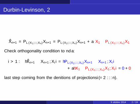
X̂n+1 = PL(X1,...,Xn)Xn+1 = PL(X2,...,Xn)Xn+1 + a(X1 − PL(X2,...,Xn)X1

)Check orthogonality condition to find a:

i > 1 : 〈X̂n+1 − Xn+1,Xi 〉 = 〈PL(X2,...,Xn)Xn+1 − Xn+1,Xi 〉+ a〈X1 − PL(X2,...,Xn)X1,Xi 〉 = 0 + 0

last step coming from the definitions of projections (i = 2 . . . n).

9 ottobre 2014 2 / 19

Durbin-Levinson, 3

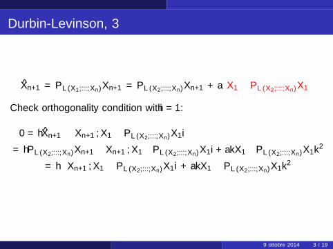
X̂n+1 = PL(X1,...,Xn)Xn+1 = PL(X2,...,Xn)Xn+1 + a(X1 − PL(X2,...,Xn)X1

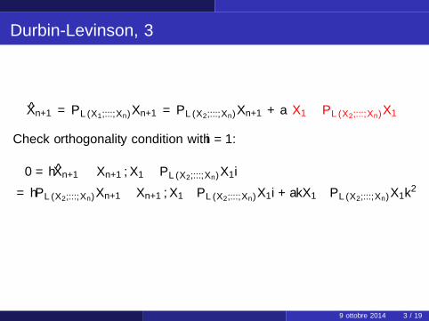
)Check orthogonality condition with i = 1:

0 = 〈X̂n+1 − Xn+1,X1 − PL(X2,...,Xn)X1〉= 〈PL(X2,...,Xn)Xn+1−Xn+1,X1−PL(X2,...,Xn)X1〉+ a‖X1−PL(X2,...,Xn)X1‖2

= −〈Xn+1,X1 − PL(X2,...,Xn)X1〉+ a‖X1 − PL(X2,...,Xn)X1‖2

=⇒ a =〈Xn+1,X1 − PL(X2,...,Xn)X1〉‖X1 − PL(X2,...,Xn)X1‖2

9 ottobre 2014 3 / 19

Durbin-Levinson, 3

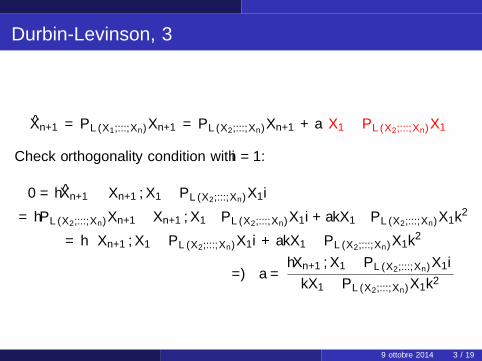
X̂n+1 = PL(X1,...,Xn)Xn+1 = PL(X2,...,Xn)Xn+1 + a(X1 − PL(X2,...,Xn)X1

)Check orthogonality condition with i = 1:

0 = 〈X̂n+1 − Xn+1,X1 − PL(X2,...,Xn)X1〉

= 〈PL(X2,...,Xn)Xn+1−Xn+1,X1−PL(X2,...,Xn)X1〉+ a‖X1−PL(X2,...,Xn)X1‖2

= −〈Xn+1,X1 − PL(X2,...,Xn)X1〉+ a‖X1 − PL(X2,...,Xn)X1‖2

=⇒ a =〈Xn+1,X1 − PL(X2,...,Xn)X1〉‖X1 − PL(X2,...,Xn)X1‖2

9 ottobre 2014 3 / 19

Durbin-Levinson, 3

X̂n+1 = PL(X1,...,Xn)Xn+1 = PL(X2,...,Xn)Xn+1 + a(X1 − PL(X2,...,Xn)X1

)Check orthogonality condition with i = 1:

0 = 〈X̂n+1 − Xn+1,X1 − PL(X2,...,Xn)X1〉= 〈PL(X2,...,Xn)Xn+1−Xn+1,X1−PL(X2,...,Xn)X1〉+ a‖X1−PL(X2,...,Xn)X1‖2

= −〈Xn+1,X1 − PL(X2,...,Xn)X1〉+ a‖X1 − PL(X2,...,Xn)X1‖2

=⇒ a =〈Xn+1,X1 − PL(X2,...,Xn)X1〉‖X1 − PL(X2,...,Xn)X1‖2

9 ottobre 2014 3 / 19

Durbin-Levinson, 3

X̂n+1 = PL(X1,...,Xn)Xn+1 = PL(X2,...,Xn)Xn+1 + a(X1 − PL(X2,...,Xn)X1

)Check orthogonality condition with i = 1:

0 = 〈X̂n+1 − Xn+1,X1 − PL(X2,...,Xn)X1〉= 〈PL(X2,...,Xn)Xn+1−Xn+1,X1−PL(X2,...,Xn)X1〉+ a‖X1−PL(X2,...,Xn)X1‖2

= −〈Xn+1,X1 − PL(X2,...,Xn)X1〉+ a‖X1 − PL(X2,...,Xn)X1‖2

=⇒ a =〈Xn+1,X1 − PL(X2,...,Xn)X1〉‖X1 − PL(X2,...,Xn)X1‖2

9 ottobre 2014 3 / 19

Durbin-Levinson, 3

X̂n+1 = PL(X1,...,Xn)Xn+1 = PL(X2,...,Xn)Xn+1 + a(X1 − PL(X2,...,Xn)X1

)Check orthogonality condition with i = 1:

0 = 〈X̂n+1 − Xn+1,X1 − PL(X2,...,Xn)X1〉= 〈PL(X2,...,Xn)Xn+1−Xn+1,X1−PL(X2,...,Xn)X1〉+ a‖X1−PL(X2,...,Xn)X1‖2

= −〈Xn+1,X1 − PL(X2,...,Xn)X1〉+ a‖X1 − PL(X2,...,Xn)X1‖2

=⇒ a =〈Xn+1,X1 − PL(X2,...,Xn)X1〉‖X1 − PL(X2,...,Xn)X1‖2

9 ottobre 2014 3 / 19

Durbin-Levinson. 4

We tried

X̂n+1 = PL(X1,...,Xn)Xn+1 = PL(X2,...,Xn)Xn+1 + a(X1 − PL(X2,...,Xn)X1

)and found

a =〈Xn+1,X1 − PL(X2,...,Xn)X1〉‖X1 − PL(X2,...,Xn)X1‖2

= 〈Xn+1,X1 − PL(X2,...,Xn)X1〉v−1n−1

withvn−1 = E(|X̂n−Xn|2) = ‖Xn−PL(X1,...,Xn−1)Xn‖2 = ‖X1−PL(X2,...,Xn)X1‖2.

We write X̂n+1 = ϕn,1Xn + · · ·+ ϕn,nX1 =n∑

j=1ϕn,jXn+1−j

so that PL(X2,...,Xn)Xn+1 =n−1∑j=1

ϕn−1,jXn+1−j

and substituting we get a recursion.

9 ottobre 2014 4 / 19

Durbin-Levinson. 4

We tried

X̂n+1 = PL(X1,...,Xn)Xn+1 = PL(X2,...,Xn)Xn+1 + a(X1 − PL(X2,...,Xn)X1

)and found

a =〈Xn+1,X1 − PL(X2,...,Xn)X1〉‖X1 − PL(X2,...,Xn)X1‖2

= 〈Xn+1,X1 − PL(X2,...,Xn)X1〉v−1n−1

withvn−1 = E(|X̂n−Xn|2) = ‖Xn−PL(X1,...,Xn−1)Xn‖2 = ‖X1−PL(X2,...,Xn)X1‖2.

We write X̂n+1 = ϕn,1Xn + · · ·+ ϕn,nX1 =n∑

j=1ϕn,jXn+1−j

so that PL(X2,...,Xn)Xn+1 =n−1∑j=1

ϕn−1,jXn+1−j

and substituting we get a recursion.

9 ottobre 2014 4 / 19

Durbin-Levinson. 4

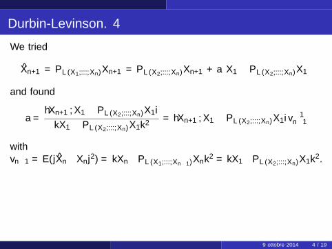
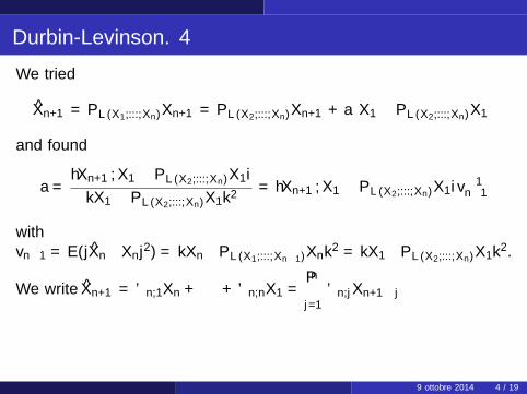
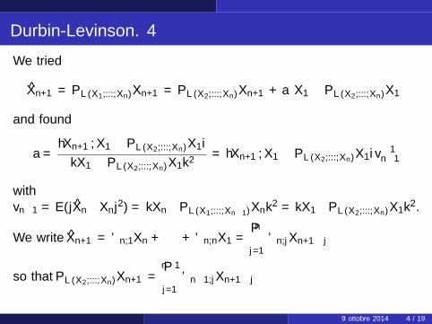
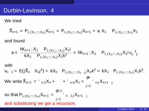
We tried

X̂n+1 = PL(X1,...,Xn)Xn+1 = PL(X2,...,Xn)Xn+1 + a(X1 − PL(X2,...,Xn)X1

)and found

a =〈Xn+1,X1 − PL(X2,...,Xn)X1〉‖X1 − PL(X2,...,Xn)X1‖2

= 〈Xn+1,X1 − PL(X2,...,Xn)X1〉v−1n−1

withvn−1 = E(|X̂n−Xn|2) = ‖Xn−PL(X1,...,Xn−1)Xn‖2 = ‖X1−PL(X2,...,Xn)X1‖2.

We write X̂n+1 = ϕn,1Xn + · · ·+ ϕn,nX1 =n∑

j=1ϕn,jXn+1−j

so that PL(X2,...,Xn)Xn+1 =n−1∑j=1

ϕn−1,jXn+1−j

and substituting we get a recursion.

9 ottobre 2014 4 / 19

Durbin-Levinson. 4

We tried

X̂n+1 = PL(X1,...,Xn)Xn+1 = PL(X2,...,Xn)Xn+1 + a(X1 − PL(X2,...,Xn)X1

)and found

a =〈Xn+1,X1 − PL(X2,...,Xn)X1〉‖X1 − PL(X2,...,Xn)X1‖2

= 〈Xn+1,X1 − PL(X2,...,Xn)X1〉v−1n−1

withvn−1 = E(|X̂n−Xn|2) = ‖Xn−PL(X1,...,Xn−1)Xn‖2 = ‖X1−PL(X2,...,Xn)X1‖2.

We write X̂n+1 = ϕn,1Xn + · · ·+ ϕn,nX1 =n∑

j=1ϕn,jXn+1−j

so that PL(X2,...,Xn)Xn+1 =n−1∑j=1

ϕn−1,jXn+1−j

and substituting we get a recursion.9 ottobre 2014 4 / 19

Durbin-Levinson algorithm. 5

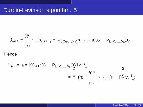
X̂n+1 =n∑

j=1

ϕn,jXn+1−j = PL(X2,...,Xn)Xn+1 + a(X1 − PL(X2,...,Xn)X1

)Hence

ϕn,n = a = 〈Xn+1,X1 − PL(X2,...,Xn)X1〉v−1n−1

=

γ(n)−n−1∑j=1

ϕn−1,jγ(n − j)

v−1n−1.

9 ottobre 2014 5 / 19

Durbin-Levinson algorithm. 6

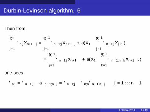
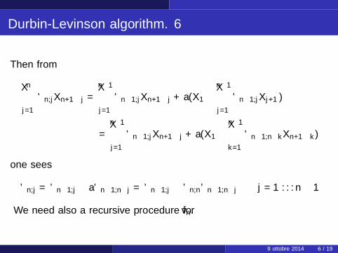
Then from

n∑j=1

ϕn,jXn+1−j =n−1∑j=1

ϕn−1,jXn+1−j + a(X1 −n−1∑j=1

ϕn−1,jXj+1)

=n−1∑j=1

ϕn−1,jXn+1−j + a(X1 −n−1∑k=1

ϕn−1,n−kXn+1−k)

one sees

ϕn,j = ϕn−1,j − aϕn−1,n−j = ϕn−1,j − ϕn,nϕn−1,n−j j = 1 . . . n − 1

We need also a recursive procedure for vn.

9 ottobre 2014 6 / 19

Durbin-Levinson algorithm. 6

Then from

n∑j=1

ϕn,jXn+1−j =n−1∑j=1

ϕn−1,jXn+1−j + a(X1 −n−1∑j=1

ϕn−1,jXj+1)

=n−1∑j=1

ϕn−1,jXn+1−j + a(X1 −n−1∑k=1

ϕn−1,n−kXn+1−k)

one sees

ϕn,j = ϕn−1,j − aϕn−1,n−j = ϕn−1,j − ϕn,nϕn−1,n−j j = 1 . . . n − 1

We need also a recursive procedure for vn.

9 ottobre 2014 6 / 19

Durbin-Levinson algorithm. 7

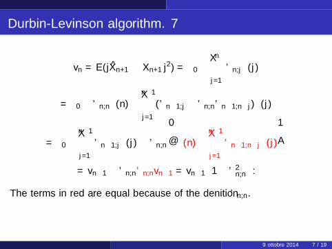
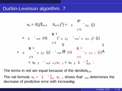
vn = E(|X̂n+1 − Xn+1|2) = γ0 −n∑

j=1

ϕn,jγ(j)

= γ0 − ϕn,nγ(n)−n−1∑j=1

(ϕn−1,j − ϕn,nϕn−1,n−j)γ(j)

= γ0 −n−1∑j=1

ϕn−1,jγ(j)− ϕn,n

γ(n)−n−1∑j=1

ϕn−1,n−jγ(j)

= vn−1 − ϕn,nϕn,nvn−1 = vn−1

(1− ϕ2

n,n

).

The terms in red are equal because of the definition ϕn,n.

The final formula vn =(1− ϕ2

n,n

)vn−1 shows that ϕn,n determines the

decrease of predictive error with increasing n.

9 ottobre 2014 7 / 19

Durbin-Levinson algorithm. 7

vn = E(|X̂n+1 − Xn+1|2) = γ0 −n∑

j=1

ϕn,jγ(j)

= γ0 − ϕn,nγ(n)−n−1∑j=1

(ϕn−1,j − ϕn,nϕn−1,n−j)γ(j)

= γ0 −n−1∑j=1

ϕn−1,jγ(j)− ϕn,n

γ(n)−n−1∑j=1

ϕn−1,n−jγ(j)

= vn−1 − ϕn,nϕn,nvn−1 = vn−1

(1− ϕ2

n,n

).

The terms in red are equal because of the definition ϕn,n.

The final formula vn =(1− ϕ2

n,n

)vn−1 shows that ϕn,n determines the

decrease of predictive error with increasing n.

9 ottobre 2014 7 / 19

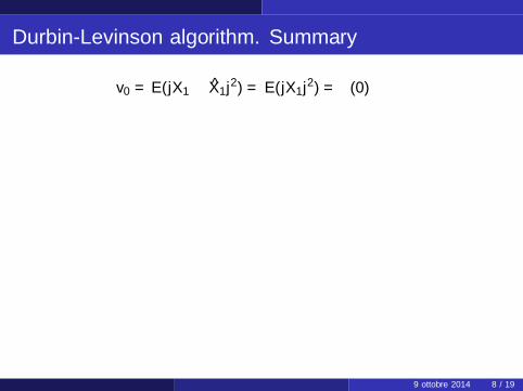
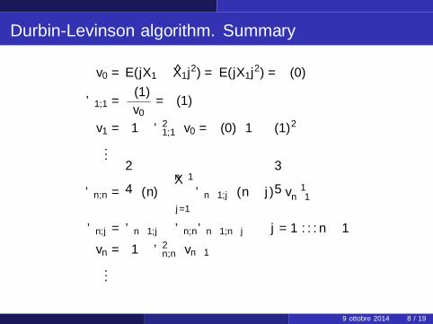
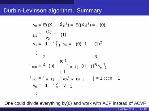
Durbin-Levinson algorithm. Summary

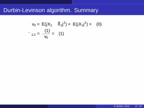
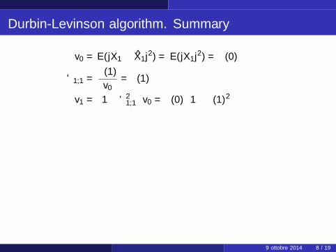
v0 = E(|X1 − X̂1|2) = E(|X1|2) = γ(0)

ϕ1,1 =γ(1)

v0= ρ(1)

v1 =(1− ϕ2

1,1

)v0 = γ(0)

(1− ρ(1)2

)...

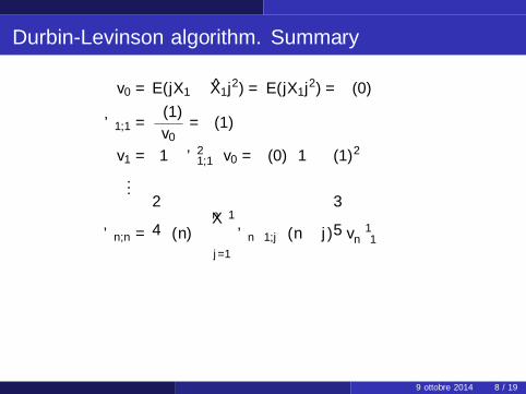
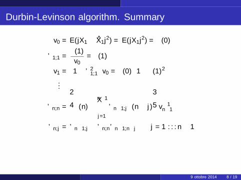
ϕn,n =

γ(n)−n−1∑j=1

ϕn−1,jγ(n − j)

v−1n−1

ϕn,j = ϕn−1,j − ϕn,nϕn−1,n−j j = 1 . . . n − 1

vn =(1− ϕ2

n,n

)vn−1

...

One could divide everything by γ(0) and work with ACF instead of ACVF

9 ottobre 2014 8 / 19

Durbin-Levinson algorithm. Summary

v0 = E(|X1 − X̂1|2) = E(|X1|2) = γ(0)

ϕ1,1 =γ(1)

v0= ρ(1)

v1 =(1− ϕ2

1,1

)v0 = γ(0)

(1− ρ(1)2

)...

ϕn,n =

γ(n)−n−1∑j=1

ϕn−1,jγ(n − j)

v−1n−1

ϕn,j = ϕn−1,j − ϕn,nϕn−1,n−j j = 1 . . . n − 1

vn =(1− ϕ2

n,n

)vn−1

...

One could divide everything by γ(0) and work with ACF instead of ACVF

9 ottobre 2014 8 / 19

Durbin-Levinson algorithm. Summary

v0 = E(|X1 − X̂1|2) = E(|X1|2) = γ(0)

ϕ1,1 =γ(1)

v0= ρ(1)

v1 =(1− ϕ2

1,1

)v0 = γ(0)

(1− ρ(1)2

)

...

ϕn,n =

γ(n)−n−1∑j=1

ϕn−1,jγ(n − j)

v−1n−1

ϕn,j = ϕn−1,j − ϕn,nϕn−1,n−j j = 1 . . . n − 1

vn =(1− ϕ2

n,n

)vn−1

...

One could divide everything by γ(0) and work with ACF instead of ACVF

9 ottobre 2014 8 / 19

Durbin-Levinson algorithm. Summary

v0 = E(|X1 − X̂1|2) = E(|X1|2) = γ(0)

ϕ1,1 =γ(1)

v0= ρ(1)

v1 =(1− ϕ2

1,1

)v0 = γ(0)

(1− ρ(1)2

)...

ϕn,n =

γ(n)−n−1∑j=1

ϕn−1,jγ(n − j)

v−1n−1

ϕn,j = ϕn−1,j − ϕn,nϕn−1,n−j j = 1 . . . n − 1

vn =(1− ϕ2

n,n

)vn−1

...

One could divide everything by γ(0) and work with ACF instead of ACVF

9 ottobre 2014 8 / 19

Durbin-Levinson algorithm. Summary

v0 = E(|X1 − X̂1|2) = E(|X1|2) = γ(0)

ϕ1,1 =γ(1)

v0= ρ(1)

v1 =(1− ϕ2

1,1

)v0 = γ(0)

(1− ρ(1)2

)...

ϕn,n =

γ(n)−n−1∑j=1

ϕn−1,jγ(n − j)

v−1n−1

ϕn,j = ϕn−1,j − ϕn,nϕn−1,n−j j = 1 . . . n − 1

vn =(1− ϕ2

n,n

)vn−1

...

One could divide everything by γ(0) and work with ACF instead of ACVF

9 ottobre 2014 8 / 19

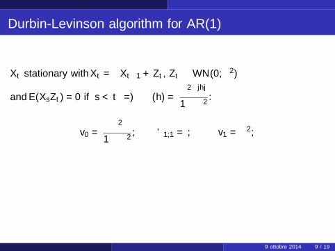
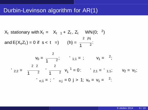
Durbin-Levinson algorithm. Summary

v0 = E(|X1 − X̂1|2) = E(|X1|2) = γ(0)

ϕ1,1 =γ(1)

v0= ρ(1)

v1 =(1− ϕ2

1,1

)v0 = γ(0)

(1− ρ(1)2

)...

ϕn,n =

γ(n)−n−1∑j=1

ϕn−1,jγ(n − j)

v−1n−1

ϕn,j = ϕn−1,j − ϕn,nϕn−1,n−j j = 1 . . . n − 1

vn =(1− ϕ2

n,n

)vn−1

...

One could divide everything by γ(0) and work with ACF instead of ACVF

9 ottobre 2014 8 / 19

Durbin-Levinson algorithm. Summary

v0 = E(|X1 − X̂1|2) = E(|X1|2) = γ(0)

ϕ1,1 =γ(1)

v0= ρ(1)

v1 =(1− ϕ2

1,1

)v0 = γ(0)

(1− ρ(1)2

)...

ϕn,n =

γ(n)−n−1∑j=1

ϕn−1,jγ(n − j)

v−1n−1

ϕn,j = ϕn−1,j − ϕn,nϕn−1,n−j j = 1 . . . n − 1

vn =(1− ϕ2

n,n

)vn−1

...

One could divide everything by γ(0) and work with ACF instead of ACVF9 ottobre 2014 8 / 19

Durbin-Levinson algorithm for AR(1)

Xt stationary with Xt = φXt−1 + Zt , Zt ∼WN(0, σ2)

and E(XsZt) = 0 if s < t

=⇒ γ(h) =σ2φ|h|

1− φ2.

v0 =σ2

1− φ2, ϕ1,1 = φ, v1 = σ2,

ϕ2,2 =

[σ2φ2

1− φ2− ϕ σ2φ

1− φ2

]v−11 = 0. ϕ2,1 = ϕ1,1, v2 = v1,

ϕn,1 = φ, ϕn,j = 0 j > 1, vn = v1 = σ2.

9 ottobre 2014 9 / 19

Durbin-Levinson algorithm for AR(1)

Xt stationary with Xt = φXt−1 + Zt , Zt ∼WN(0, σ2)

and E(XsZt) = 0 if s < t =⇒ γ(h) =σ2φ|h|

1− φ2.

v0 =σ2

1− φ2, ϕ1,1 = φ, v1 = σ2,

ϕ2,2 =

[σ2φ2

1− φ2− ϕ σ2φ

1− φ2

]v−11 = 0. ϕ2,1 = ϕ1,1, v2 = v1,

ϕn,1 = φ, ϕn,j = 0 j > 1, vn = v1 = σ2.

9 ottobre 2014 9 / 19

Durbin-Levinson algorithm for AR(1)

Xt stationary with Xt = φXt−1 + Zt , Zt ∼WN(0, σ2)

and E(XsZt) = 0 if s < t =⇒ γ(h) =σ2φ|h|

1− φ2.

v0 =σ2

1− φ2, ϕ1,1 = φ, v1 = σ2,

ϕ2,2 =

[σ2φ2

1− φ2− ϕ σ2φ

1− φ2

]v−11 = 0. ϕ2,1 = ϕ1,1, v2 = v1,

ϕn,1 = φ, ϕn,j = 0 j > 1, vn = v1 = σ2.

9 ottobre 2014 9 / 19

Durbin-Levinson algorithm for AR(1)

Xt stationary with Xt = φXt−1 + Zt , Zt ∼WN(0, σ2)

and E(XsZt) = 0 if s < t =⇒ γ(h) =σ2φ|h|

1− φ2.

v0 =σ2

1− φ2, ϕ1,1 = φ, v1 = σ2,

ϕ2,2 =

[σ2φ2

1− φ2− ϕ σ2φ

1− φ2

]v−11 = 0. ϕ2,1 = ϕ1,1, v2 = v1,

ϕn,1 = φ, ϕn,j = 0 j > 1, vn = v1 = σ2.

9 ottobre 2014 9 / 19

Durbin-Levinson algorithm for MA(1)

Xt = Zt − ϑZt−1, Zt ∼WN(0, σ2), γ(0) = σ2(1 + ϑ2), γ(1) = −σ2ϑ.

v0 = σ2(1 + ϑ2) ϕ1,1 = − ϑ

1 + ϑ2

v1 =σ2(1 + ϑ2 + ϑ4)

1 + ϑ2ϕ2,2 = − ϑ2

1 + ϑ2 + ϑ4. . .

v2 =σ2(1 + ϑ2 + ϑ4 + ϑ6)

1 + ϑ2 + ϑ4. . .

Remarks: Computations are long and tedious.vn converges (slowly) towards σ2 (the white-noise variance) if |ϑ| < 1.

9 ottobre 2014 10 / 19

Durbin-Levinson algorithm for MA(1)

Xt = Zt − ϑZt−1, Zt ∼WN(0, σ2), γ(0) = σ2(1 + ϑ2), γ(1) = −σ2ϑ.

v0 = σ2(1 + ϑ2) ϕ1,1 = − ϑ

1 + ϑ2

v1 =σ2(1 + ϑ2 + ϑ4)

1 + ϑ2ϕ2,2 = − ϑ2

1 + ϑ2 + ϑ4. . .

v2 =σ2(1 + ϑ2 + ϑ4 + ϑ6)

1 + ϑ2 + ϑ4. . .

Remarks: Computations are long and tedious.vn converges (slowly) towards σ2 (the white-noise variance) if |ϑ| < 1.

9 ottobre 2014 10 / 19

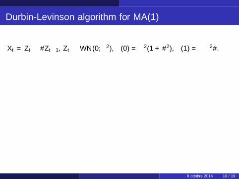
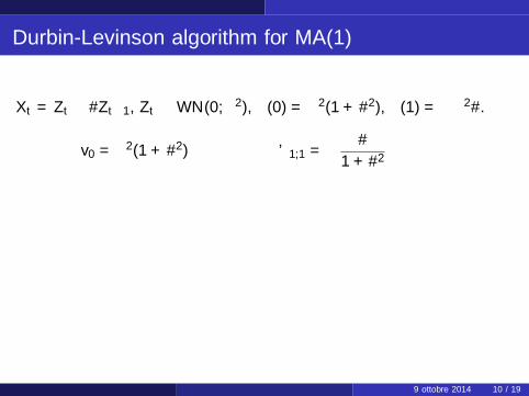
Durbin-Levinson algorithm for MA(1)

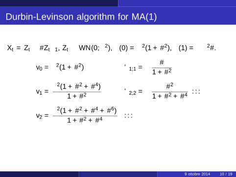
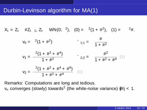
Xt = Zt − ϑZt−1, Zt ∼WN(0, σ2), γ(0) = σ2(1 + ϑ2), γ(1) = −σ2ϑ.

v0 = σ2(1 + ϑ2) ϕ1,1 = − ϑ

1 + ϑ2

v1 =σ2(1 + ϑ2 + ϑ4)

1 + ϑ2ϕ2,2 = − ϑ2

1 + ϑ2 + ϑ4. . .

v2 =σ2(1 + ϑ2 + ϑ4 + ϑ6)

1 + ϑ2 + ϑ4. . .

Remarks: Computations are long and tedious.vn converges (slowly) towards σ2 (the white-noise variance) if |ϑ| < 1.

9 ottobre 2014 10 / 19

Durbin-Levinson algorithm for MA(1)

Xt = Zt − ϑZt−1, Zt ∼WN(0, σ2), γ(0) = σ2(1 + ϑ2), γ(1) = −σ2ϑ.

v0 = σ2(1 + ϑ2) ϕ1,1 = − ϑ

1 + ϑ2

v1 =σ2(1 + ϑ2 + ϑ4)

1 + ϑ2ϕ2,2 = − ϑ2

1 + ϑ2 + ϑ4. . .

v2 =σ2(1 + ϑ2 + ϑ4 + ϑ6)

1 + ϑ2 + ϑ4. . .

Remarks: Computations are long and tedious.vn converges (slowly) towards σ2 (the white-noise variance) if |ϑ| < 1.

9 ottobre 2014 10 / 19

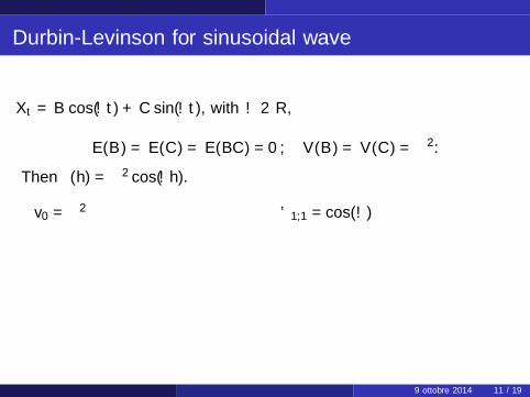
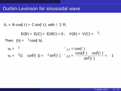
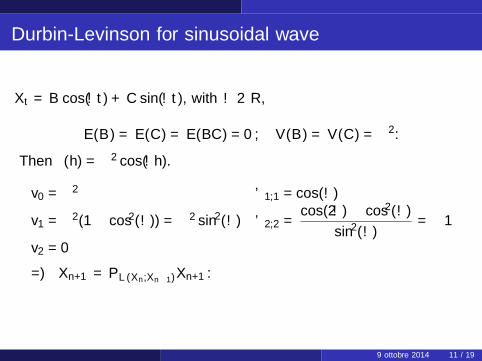
Durbin-Levinson for sinusoidal wave

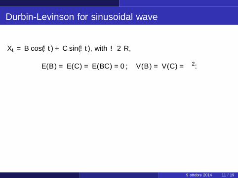
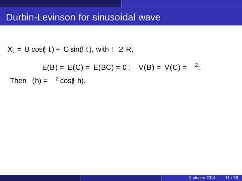
Xt = B cos(ωt) + C sin(ωt), with ω ∈ R,

E(B) = E(C ) = E(BC ) = 0, V(B) = V(C ) = σ2.

Then γ(h) = σ2 cos(ωh).

v0 = σ2 ϕ1,1 = cos(ω)

v1 = σ2(1− cos2(ω)) = σ2 sin2(ω) ϕ2,2 =cos(2ω)− cos2(ω)

sin2(ω)= −1

v2 = 0

=⇒ Xn+1 = PL(Xn,Xn−1)Xn+1.

9 ottobre 2014 11 / 19

Durbin-Levinson for sinusoidal wave

Xt = B cos(ωt) + C sin(ωt), with ω ∈ R,

E(B) = E(C ) = E(BC ) = 0, V(B) = V(C ) = σ2.

Then γ(h) = σ2 cos(ωh).

v0 = σ2 ϕ1,1 = cos(ω)

v1 = σ2(1− cos2(ω)) = σ2 sin2(ω) ϕ2,2 =cos(2ω)− cos2(ω)

sin2(ω)= −1

v2 = 0

=⇒ Xn+1 = PL(Xn,Xn−1)Xn+1.

9 ottobre 2014 11 / 19

Durbin-Levinson for sinusoidal wave

Xt = B cos(ωt) + C sin(ωt), with ω ∈ R,

E(B) = E(C ) = E(BC ) = 0, V(B) = V(C ) = σ2.

Then γ(h) = σ2 cos(ωh).

v0 = σ2 ϕ1,1 = cos(ω)

v1 = σ2(1− cos2(ω)) = σ2 sin2(ω) ϕ2,2 =cos(2ω)− cos2(ω)

sin2(ω)= −1

v2 = 0

=⇒ Xn+1 = PL(Xn,Xn−1)Xn+1.

9 ottobre 2014 11 / 19

Durbin-Levinson for sinusoidal wave

Xt = B cos(ωt) + C sin(ωt), with ω ∈ R,

E(B) = E(C ) = E(BC ) = 0, V(B) = V(C ) = σ2.

Then γ(h) = σ2 cos(ωh).

v0 = σ2 ϕ1,1 = cos(ω)

v1 = σ2(1− cos2(ω)) = σ2 sin2(ω) ϕ2,2 =cos(2ω)− cos2(ω)

sin2(ω)= −1

v2 = 0

=⇒ Xn+1 = PL(Xn,Xn−1)Xn+1.

9 ottobre 2014 11 / 19

Durbin-Levinson for sinusoidal wave

Xt = B cos(ωt) + C sin(ωt), with ω ∈ R,

E(B) = E(C ) = E(BC ) = 0, V(B) = V(C ) = σ2.

Then γ(h) = σ2 cos(ωh).

v0 = σ2 ϕ1,1 = cos(ω)

v1 = σ2(1− cos2(ω)) = σ2 sin2(ω) ϕ2,2 =cos(2ω)− cos2(ω)

sin2(ω)= −1

v2 = 0

=⇒ Xn+1 = PL(Xn,Xn−1)Xn+1.

9 ottobre 2014 11 / 19

Partial auto-correlation

For a stationary process {Xt} α(h) the partial auto-correlation representsthe correlation between Xt and Xt+h, after removing the effect ofintermediate values.

Definition: α(1) = ρ(Xt ,Xt+1) = ρ(1).

α(h) = ρ(Xt −PL(Xt+1,...,Xt+h−1)Xt ,Xt+h−PL(Xt+1,...,Xt+h−1)Xt+h) h > 1.

α(h) =E((Xt − PL(Xt+1,...,Xt+h−1)Xt)(Xt+h − PL(Xt+1,...,Xt+h−1)Xt+h))

V(Xt − PL(Xt+1,...,Xt+h−1)Xt)

=〈X1 − PL(X2,...,Xh)X1,Xh+1 − PL(X2,...,Xh)Xh+1〉

‖X1 − PL(X2,...,Xh)X1‖2

=〈X1,Xh+1 − PL(X2,...,Xh)Xh+1〉‖X1 − PL(X2,...,Xh)X1‖2

= ϕh,h.

Durbin-Levinson’s algorithm is a method to compute α(·).

9 ottobre 2014 12 / 19

Partial auto-correlation

For a stationary process {Xt} α(h) the partial auto-correlation representsthe correlation between Xt and Xt+h, after removing the effect ofintermediate values.Definition: α(1) = ρ(Xt ,Xt+1) = ρ(1).

α(h) = ρ(Xt −PL(Xt+1,...,Xt+h−1)Xt ,Xt+h−PL(Xt+1,...,Xt+h−1)Xt+h) h > 1.

α(h) =E((Xt − PL(Xt+1,...,Xt+h−1)Xt)(Xt+h − PL(Xt+1,...,Xt+h−1)Xt+h))

V(Xt − PL(Xt+1,...,Xt+h−1)Xt)

=〈X1 − PL(X2,...,Xh)X1,Xh+1 − PL(X2,...,Xh)Xh+1〉

‖X1 − PL(X2,...,Xh)X1‖2

=〈X1,Xh+1 − PL(X2,...,Xh)Xh+1〉‖X1 − PL(X2,...,Xh)X1‖2

= ϕh,h.

Durbin-Levinson’s algorithm is a method to compute α(·).

9 ottobre 2014 12 / 19

Partial auto-correlation

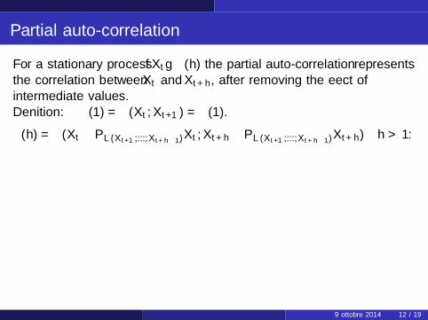
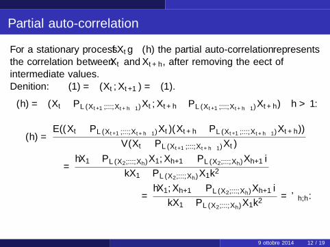
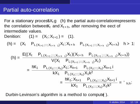
For a stationary process {Xt} α(h) the partial auto-correlation representsthe correlation between Xt and Xt+h, after removing the effect ofintermediate values.Definition: α(1) = ρ(Xt ,Xt+1) = ρ(1).

α(h) = ρ(Xt −PL(Xt+1,...,Xt+h−1)Xt ,Xt+h−PL(Xt+1,...,Xt+h−1)Xt+h) h > 1.

α(h) =E((Xt − PL(Xt+1,...,Xt+h−1)Xt)(Xt+h − PL(Xt+1,...,Xt+h−1)Xt+h))

V(Xt − PL(Xt+1,...,Xt+h−1)Xt)

=〈X1 − PL(X2,...,Xh)X1,Xh+1 − PL(X2,...,Xh)Xh+1〉

‖X1 − PL(X2,...,Xh)X1‖2

=〈X1,Xh+1 − PL(X2,...,Xh)Xh+1〉‖X1 − PL(X2,...,Xh)X1‖2

= ϕh,h.

Durbin-Levinson’s algorithm is a method to compute α(·).

9 ottobre 2014 12 / 19

Partial auto-correlation

For a stationary process {Xt} α(h) the partial auto-correlation representsthe correlation between Xt and Xt+h, after removing the effect ofintermediate values.Definition: α(1) = ρ(Xt ,Xt+1) = ρ(1).

α(h) = ρ(Xt −PL(Xt+1,...,Xt+h−1)Xt ,Xt+h−PL(Xt+1,...,Xt+h−1)Xt+h) h > 1.

α(h) =E((Xt − PL(Xt+1,...,Xt+h−1)Xt)(Xt+h − PL(Xt+1,...,Xt+h−1)Xt+h))

V(Xt − PL(Xt+1,...,Xt+h−1)Xt)

=〈X1 − PL(X2,...,Xh)X1,Xh+1 − PL(X2,...,Xh)Xh+1〉

‖X1 − PL(X2,...,Xh)X1‖2

=〈X1,Xh+1 − PL(X2,...,Xh)Xh+1〉‖X1 − PL(X2,...,Xh)X1‖2

= ϕh,h.

Durbin-Levinson’s algorithm is a method to compute α(·).

9 ottobre 2014 12 / 19

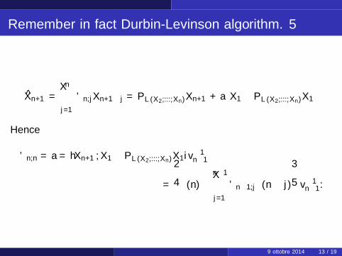
Remember in fact Durbin-Levinson algorithm. 5

X̂n+1 =n∑

j=1

ϕn,jXn+1−j = PL(X2,...,Xn)Xn+1 + a(X1 − PL(X2,...,Xn)X1

)Hence

ϕn,n = a = 〈Xn+1,X1 − PL(X2,...,Xn)X1〉v−1n−1

=

γ(n)−n−1∑j=1

ϕn−1,jγ(n − j)

v−1n−1.

9 ottobre 2014 13 / 19

Examples of PACF

{Xt} AR(1), =⇒ α(1) = φ, α(h) = 0 for h > 1 (seen before).

{Xt} AR(p), i.e. stationary proces s.t.

Xt =

p∑k=1

φkXt−k + Zt , {Zt} ∼WN(0, σ2).

If t ≥ p, PL(X1,...,Xt)Xt+1 =∑p

k=1 φkXt+1−k (check).

Then ϕp,p = α(p) = φp, ϕh,h = 0 if h > p, i.e. α(h) = 0 for h > p.

{Xt} MA(1) =⇒ α(h) = −ϑh/(1 + ϑ2 + · · ·+ ϑ2h) (longcomputation)

PACF of AR processes has finite support, while PACF of MA is alwaysnon-zero. This is the opposite as for ACF.

Sample PACF. Apply Durbin-Levinson algorithm to γ̂(·).

9 ottobre 2014 14 / 19

Examples of PACF

{Xt} AR(1), =⇒ α(1) = φ, α(h) = 0 for h > 1 (seen before).

{Xt} AR(p), i.e. stationary proces s.t.

Xt =

p∑k=1

φkXt−k + Zt , {Zt} ∼WN(0, σ2).

If t ≥ p, PL(X1,...,Xt)Xt+1 =∑p

k=1 φkXt+1−k (check).

Then ϕp,p = α(p) = φp, ϕh,h = 0 if h > p, i.e. α(h) = 0 for h > p.

{Xt} MA(1) =⇒ α(h) = −ϑh/(1 + ϑ2 + · · ·+ ϑ2h) (longcomputation)

PACF of AR processes has finite support, while PACF of MA is alwaysnon-zero. This is the opposite as for ACF.

Sample PACF. Apply Durbin-Levinson algorithm to γ̂(·).

9 ottobre 2014 14 / 19

Examples of PACF

{Xt} AR(1), =⇒ α(1) = φ, α(h) = 0 for h > 1 (seen before).

{Xt} AR(p), i.e. stationary proces s.t.

Xt =

p∑k=1

φkXt−k + Zt , {Zt} ∼WN(0, σ2).

If t ≥ p, PL(X1,...,Xt)Xt+1 =∑p

k=1 φkXt+1−k (check).

Then ϕp,p = α(p) = φp, ϕh,h = 0 if h > p, i.e. α(h) = 0 for h > p.

{Xt} MA(1) =⇒ α(h) = −ϑh/(1 + ϑ2 + · · ·+ ϑ2h) (longcomputation)

PACF of AR processes has finite support, while PACF of MA is alwaysnon-zero. This is the opposite as for ACF.

Sample PACF. Apply Durbin-Levinson algorithm to γ̂(·).

9 ottobre 2014 14 / 19

Examples of PACF

{Xt} AR(1), =⇒ α(1) = φ, α(h) = 0 for h > 1 (seen before).

{Xt} AR(p), i.e. stationary proces s.t.

Xt =

p∑k=1

φkXt−k + Zt , {Zt} ∼WN(0, σ2).

If t ≥ p, PL(X1,...,Xt)Xt+1 =∑p

k=1 φkXt+1−k (check).

Then ϕp,p = α(p) = φp, ϕh,h = 0 if h > p, i.e. α(h) = 0 for h > p.

{Xt} MA(1) =⇒ α(h) = −ϑh/(1 + ϑ2 + · · ·+ ϑ2h) (longcomputation)

PACF of AR processes has finite support, while PACF of MA is alwaysnon-zero. This is the opposite as for ACF.

Sample PACF. Apply Durbin-Levinson algorithm to γ̂(·).

9 ottobre 2014 14 / 19

Examples of PACF

{Xt} AR(1), =⇒ α(1) = φ, α(h) = 0 for h > 1 (seen before).

{Xt} AR(p), i.e. stationary proces s.t.

Xt =

p∑k=1

φkXt−k + Zt , {Zt} ∼WN(0, σ2).

If t ≥ p, PL(X1,...,Xt)Xt+1 =∑p

k=1 φkXt+1−k (check).

Then ϕp,p = α(p) = φp, ϕh,h = 0 if h > p, i.e. α(h) = 0 for h > p.

{Xt} MA(1) =⇒ α(h) = −ϑh/(1 + ϑ2 + · · ·+ ϑ2h) (longcomputation)

PACF of AR processes has finite support, while PACF of MA is alwaysnon-zero. This is the opposite as for ACF.

Sample PACF. Apply Durbin-Levinson algorithm to γ̂(·).

9 ottobre 2014 14 / 19

Examples of PACF

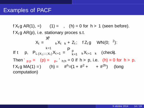
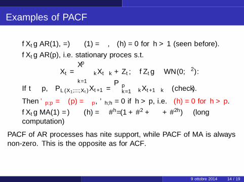
{Xt} AR(1), =⇒ α(1) = φ, α(h) = 0 for h > 1 (seen before).

{Xt} AR(p), i.e. stationary proces s.t.

Xt =

p∑k=1

φkXt−k + Zt , {Zt} ∼WN(0, σ2).

If t ≥ p, PL(X1,...,Xt)Xt+1 =∑p

k=1 φkXt+1−k (check).

Then ϕp,p = α(p) = φp, ϕh,h = 0 if h > p, i.e. α(h) = 0 for h > p.

{Xt} MA(1) =⇒ α(h) = −ϑh/(1 + ϑ2 + · · ·+ ϑ2h) (longcomputation)

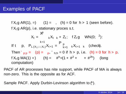
PACF of AR processes has finite support, while PACF of MA is alwaysnon-zero. This is the opposite as for ACF.

Sample PACF. Apply Durbin-Levinson algorithm to γ̂(·).

9 ottobre 2014 14 / 19

Examples of PACF

{Xt} AR(1), =⇒ α(1) = φ, α(h) = 0 for h > 1 (seen before).

{Xt} AR(p), i.e. stationary proces s.t.

Xt =

p∑k=1

φkXt−k + Zt , {Zt} ∼WN(0, σ2).

If t ≥ p, PL(X1,...,Xt)Xt+1 =∑p

k=1 φkXt+1−k (check).

Then ϕp,p = α(p) = φp, ϕh,h = 0 if h > p, i.e. α(h) = 0 for h > p.

{Xt} MA(1) =⇒ α(h) = −ϑh/(1 + ϑ2 + · · ·+ ϑ2h) (longcomputation)

PACF of AR processes has finite support, while PACF of MA is alwaysnon-zero. This is the opposite as for ACF.

Sample PACF. Apply Durbin-Levinson algorithm to γ̂(·).

9 ottobre 2014 14 / 19

Sample ACF and PACF

0 5 10 15

-0.5

0.0

0.5

1.0

Lag

ACF

Oveshort data

5 10 15

-0.4

0.0

0.2

Lag

Par

tial A

CF

9 ottobre 2014 15 / 19

Sample ACF of Huron: AR(1) fit

0 5 10 15

-0.4

-0.2

0.0

0.2

0.4

0.6

0.8

1.0

Lag

ACF

ACF of detrended Huron data

9 ottobre 2014 16 / 19

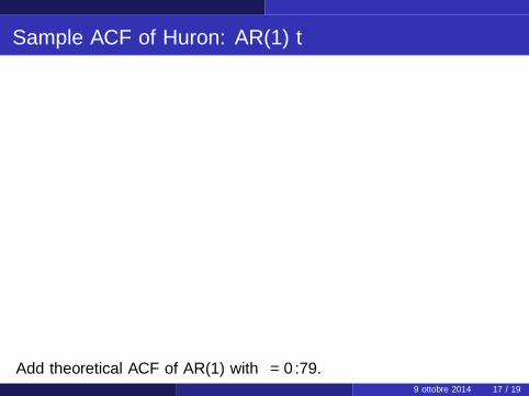
Sample ACF of Huron: AR(1) fit

0 5 10 15

-0.4

-0.2

0.0

0.2

0.4

0.6

0.8

1.0

Lag

ACF

ACF of detrended Huron data

Add theoretical ACF of AR(1) with φ = 0.79.9 ottobre 2014 17 / 19

Sample ACF of Huron: AR(1) fit

0 5 10 15

-0.4

-0.2

0.0

0.2

0.4

0.6

0.8

1.0

Lag

ACF

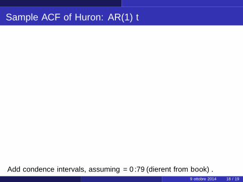
ACF of detrended Huron data

Add confidence intervals, assuming φ = 0.79 (different from book).9 ottobre 2014 18 / 19

Sample ACF and PACF of Huron data

0 5 10 15

-0.2

0.2

0.6

1.0

Lag

ACF

Huron data

5 10 15

-0.2

0.2

0.6

Lag

Par

tial A

CF

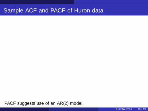
PACF suggests use of an AR(2) model.9 ottobre 2014 19 / 19