Vol.:(0123456789)1 3

J Mar Sci Technol (2017) 22:655–672 DOI 10.1007/s00773-017-0440-3

ORIGINAL ARTICLE

Dynamic behaviour of anchor handling vessels during anchor deployment

Xiaopeng Wu1 · Torgeir Moan1,2,3 

Received: 3 April 2016 / Accepted: 24 February 2017 / Published online: 24 March 2017 © The Author(s) 2017. This article is published with open access at Springerlink.com

1 Introduction

Drilling rigs operate at many different sites and are, there-fore, often moved. Such operations are typically called the Rig Move Operations (RMO). Anchor Handling Opera-tion (AHO) is a crucial part within a RMO for rigs posi-tioned by mooring systems, involving anchor deployment, anchor retrieval, rig towing, etc. Other operations like pipe-laying operation and offshore wind turbine installa-tion require AHO as well. Therefore, AHO is one of the most common offshore operations. As the offshore oil and gas industry move into deeper water, and the offshore wind energy becomes more promising, the number of anchor line positioning systems are increasing. Therefore, even more AHOs are expected in future.

Anchor handling operation is also inherently hazardous and could lead to fatal consequences, as experienced, e.g., with the Bourbon Dolphin accident in 2007 [1]. The anchor handling vessel (AHV) Bourbon Dolphin capsized during anchor deployment in the Rosebank oilfield due to a series of complex circumstances. Another AHV, Stevns Power, lost stability during anchor retrieval in 2003 [2]. Despite only two instances of capsizing AHVs in the past decade, both of the accidents resulted in casualties. Therefore, it is crucial to enhance the safety of AHOs.

As AHOs are more frequently performed in deeper waters with stricter requirements, the capacity of the AHVs is significantly higher than before. Modern AHVs are equipped with bigger engines for higher bol-lard pull (the maximum pulling force that a vessel can exert on another vessel or object), larger winches with higher capacity and a larger deck for storing more equip-ments. To insert alternative links on the mooring line or to increase the mooring line length beyond the capacity of the rig’s anchor winches, modern AHVs have double

Abstract Anchor handling operation (AHO) is poten-tially hazardous, as for instance demonstrated by the Bour-bon Dolphin accident in 2007. Although the accident has been studied by various parties, there has been limited focus on the dynamic behaviour of an anchor handling vessel (AHV) during anchor deployment. In this paper, a numerical model and an analysis procedure are proposed to study the motion of the AHV and especially the influence of the tension in the mooring line. The operation is divided into stages and assumed to be stationary within each stage. The emphasis was placed on the vessel behaviour in waves, although the model and the procedure can also be used to study wind and current effects. In addition, the need for improving current practice of anchor handling operation planning in the view of the methodology outlined is dis-cussed. Finally, the development of operational criteria for AHO is addressed.

Keywords Anchor handling operation · Simulation · Motion analysis · Planning of operation · Criteria

* Xiaopeng Wu xiaopeng.wu@ntnu.no

1 Centre for Ships and Ocean Structures (CeSOS), NTNU, Trondheim, Norway

2 Centre for Autonomous Marine Operations and Systems (AMOS), NTNU, Trondheim, Norway

3 Department of Marine Technology, NTNU, Trondheim, Norway

656 J Mar Sci Technol (2017) 22:655–672

1 3

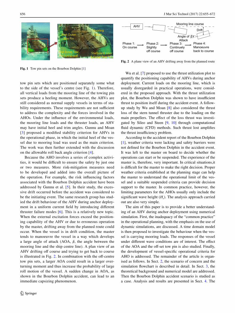
tow pin sets which are positioned separately some what to the side of the vessel’s centre (see Fig. 1). Therefore, all vertical loads from the mooring line of the towing pin sets produce a heeling moment. However, the AHVs are still considered as normal supply vessels in terms of sta-bility requirements. These requirements are not sufficient to address the complexity and the forces involved in the AHOs. Under the influence of the environmental loads, the mooring line loads and the thruster loads, an AHV may have initial heel and trim angles. Gunnu and Moan [3] proposed a modified stability criterion for AHVs in the operational phase, in which the initial heel of the ves-sel due to mooring load was used as the main criterion. The work was then further extended with the discussion on the allowable roll back angle criterion [4].

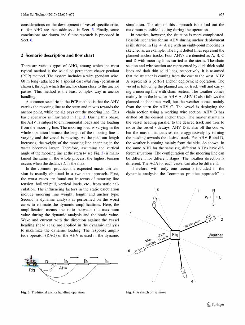
Because the AHO involves a series of complex activi-ties, it would be difficult to ensure the safety by just one or two measures. More risk-mitigation measures need to be developed and added into the overall picture of the operation. For example, the risk influencing factors associated with the Bourbon Dolphin accident have been addressed by Gunnu et  al. [5]. In their study, the exces-sive drift occurred before the accident was considered to be the initiating event. The same research group has stud-ied the drift behaviour of the AHV during anchor deploy-ment in a uniform current field by introducing different thruster failure modes [6]. This is a relatively new topic. When the external excitation forces exceed the position-ing capability of the AHV or due to erroneous operation by the master, drifting away from the planned route could occur. When the vessel is in drift condition, the master tends to manoeuvre the vessel in a way which develops a large angle of attack (AOA, �, the angle between the mooring line and the ship centre line). A plan view of an AHV drifting off course and trying to get back to course is illustrated in Fig. 2. In combination with the off-centre tow pin sets, a larger AOA could result in a larger over-turning moment and thus increase the probability of large roll motion of the vessel. A sudden change in AOA, as shown in the Bourbon Dolphin accident, can lead to an immediate capsizing phenomenon.

Wu et al. [7] proposed to use the thrust utilization plot to quantify the positioning capability of AHVs during anchor deployment. Current loads on the mooring line, which is usually disregarded in practical operations, were consid-ered in the proposed approach. With the thrust utilization plot, the Bourbon Dolphin was shown to have insufficient thrust to position itself during the accident event. A follow-up study by Wu and Moan [8] also considered the thrust loss of the stern tunnel thruster due to the loading on the main propellers. The effect of the loss thrust was investi-gated by Sileo and Steen [9, 10] through computational fluid dynamic (CFD) methods. Such thrust lost amplifies the thrust insufficiency problem.

According to the accident report of the Bourbon Dolphin [1], weather criteria were lacking and safety barriers were not defined for the Bourbon Dolphin in the accident event. It was left to the master on board to decide whether the operations can start or be suspended. The experience of the master is, therefore, very important. In critical situations,it is difficult for the master to make the right decision. Proper weather criteria established at the planning stage can help the master to understand the operational limit of the ves-sel and a suitable suspended criteria can provide decision support to the master. In common practice, however, the limiting parameters for the AHOs usually only include the significant wave height (Hs). The analysis approach carried out are also very simple.

The aim of this paper is to provide a better understand-ing of an AHV during anchor deployment using numerical simulation. First, the inadequacy of the “common practice” in the operational planning, with the emphasis on the use of dynamic simulations, are discussed. A time domain model is then proposed to investigate the behaviour when the ves-sel is carrying mooring loads. The responses of the vessel under different wave conditions are of interest. The effect of the AOA and the off-set tow pin is also studied. Finally, the development of vessel-specific operational criteria for AHO is addressed. The remainder of the article is organ-ised as follows. In Sect. 2, the scenario of concern and the simulation flowchart is described in detail. In Sect. 3, the theoretical background and numerical model are addressed. Then the Bourbon Dolphin accident scenario is studied as a case. Analysis and results are presented in Sect.  4. The

MooringChainPort Outer

Tow Pin

Starboard Inner& Outer Tow Pins

Port Inner TowPin (retracted)

Fig. 1 Tow pin sets on the Bourbon Dolphin [1]

Phase 1:On course

Phase 2:Slightlyoff course

Phase 3:Continuelyoff course

Phase 4:Manoeuvre back to course

βAngle ofAttack

Drift

Mooring line courseAHV

Fig. 2 A plane view of an AHV drifting away from the planned route

657J Mar Sci Technol (2017) 22:655–672

1 3

considerations on the development of vessel-specific crite-ria for AHO are then addressed in Sect.  5. Finally, some conclusions are drawn and future research is proposed in Sect. 6.

2 Scenario description and flow chart

There are various types of AHO, among which the most typical method is the so-called permanent chaser pendant (PCP) method. The system includes a wire (pendant wire, 60 m long) attached to a special cast oval ring (permanent chaser), through which the anchor chain close to the anchor passes. This method is the least complex way in anchor handling.

A common scenario in the PCP method is that the AHV carries the mooring line at the stern and moves towards the anchor point, while the rig pays out the mooring line. This basic scenarios is illustrated in Fig.  3. During this phase, the AHV is subject to environmental loads and the loading from the mooring line. The mooring load is varying in the whole operation because the length of the mooring line is varying and the vessel is moving. As the paid-out length increases, the weight of the mooring line spanning in the water becomes larger. Therefore, assuming the vertical angle of the mooring line at the stern (� see Fig. 3) is main-tained the same in the whole process, the highest tension occurs when the distance D is the max.

In the common practice, the expected maximum ten-sion is usually obtained in a two-step approach. First, the worst cases are found out in terms of mooring line tension, bollard pull, vertical loads, etc., from static cal-culation. The influencing factors in the static calculation include mooring line weight, length and anchor type. Second, a dynamic analysis is performed on the worst cases to estimate the dynamic amplifications. Here, the amplification means the ratio between the maximum value during the dynamic analysis and the static value. Wave and current with the direction against the vessel heading (head seas) are applied in the dynamic analysis to maximize the dynamic loading. The response ampli-tude operator (RAO) of the AHV is used in the dynamic

simulation. The aim of this approach is to find out the maximum possible loading during the operation.

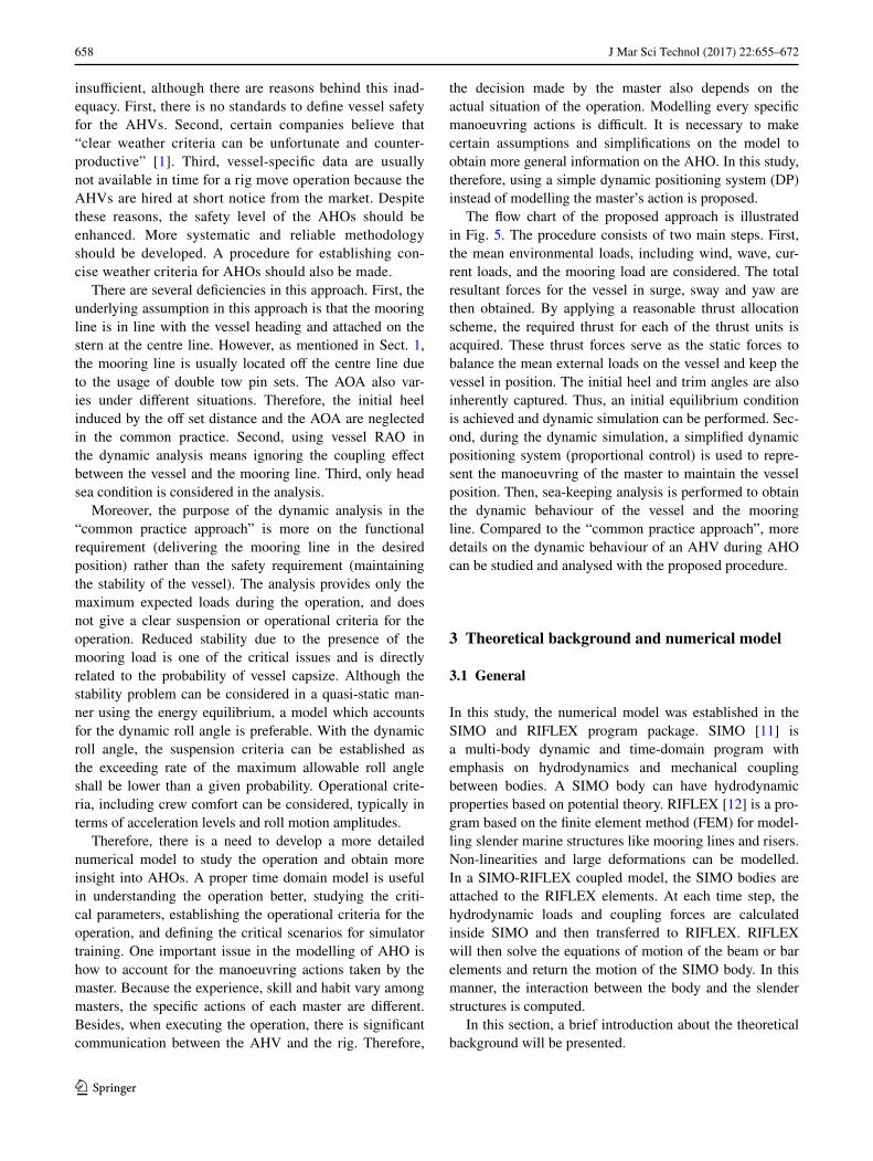
In practice, however, the situation is more complicated. Possible scenarios for an AHV during anchor deployment is illustrated in Fig. 4. A rig with an eight-point mooring is sketched as an example. The light dotted lines represent the planned anchor tracks. Four AHVs are denoted as A, B, C and D with mooring lines carried at the sterns. The chain section and wire section are represented by dark thick solid lines and dark thin solid lines, respectively. It is assumed that the weather is coming from the east to the west. AHV A represents a perfect anchor deployment operation. The vessel is following the planned anchor track well and carry-ing a mooring line with chain section. The weather comes mainly from the bow for AHV A. AHV C also follows the planned anchor track well, but the weather comes mainly from the stern for AHV C. The vessel is deploying the chain section using a working wire section. AHV B has drifted off the desired anchor track. The master maintains the vessel heading parallel to the desired track and tries to move the vessel sideways. AHV D is also off the course, but the master manoeuvres more aggressively by turning the heading towards the desired track. For AHV B and D, the weather is coming mainly from the side. As shown, in the same AHO for the same rig, different AHVs have dif-ferent situations. The configuration of the mooring line can be different for different stages. The weather direction is different. The AOA for each vessel can also be different.

Therefore, with only one scenario included in the dynamic analysis, the “common practice approach” is

αD

AHVRig

Fig. 3 Traditional anchor handling operation

Rig

1

2

3

45

6

7

8 N

S

W E

AHV

Mooring line A

B

D

C

Weather Chain

Section Wire

Section

Fig. 4 A sketch of rig move

658 J Mar Sci Technol (2017) 22:655–672

1 3

insufficient, although there are reasons behind this inad-equacy. First, there is no standards to define vessel safety for the AHVs. Second, certain companies believe that “clear weather criteria can be unfortunate and counter-productive” [1]. Third, vessel-specific data are usually not available in time for a rig move operation because the AHVs are hired at short notice from the market. Despite these reasons, the safety level of the AHOs should be enhanced. More systematic and reliable methodology should be developed. A procedure for establishing con-cise weather criteria for AHOs should also be made.

There are several deficiencies in this approach. First, the underlying assumption in this approach is that the mooring line is in line with the vessel heading and attached on the stern at the centre line. However, as mentioned in Sect. 1, the mooring line is usually located off the centre line due to the usage of double tow pin sets. The AOA also var-ies under different situations. Therefore, the initial heel induced by the off set distance and the AOA are neglected in the common practice. Second, using vessel RAO in the dynamic analysis means ignoring the coupling effect between the vessel and the mooring line. Third, only head sea condition is considered in the analysis.

Moreover, the purpose of the dynamic analysis in the “common practice approach” is more on the functional requirement (delivering the mooring line in the desired position) rather than the safety requirement (maintaining the stability of the vessel). The analysis provides only the maximum expected loads during the operation, and does not give a clear suspension or operational criteria for the operation. Reduced stability due to the presence of the mooring load is one of the critical issues and is directly related to the probability of vessel capsize. Although the stability problem can be considered in a quasi-static man-ner using the energy equilibrium, a model which accounts for the dynamic roll angle is preferable. With the dynamic roll angle, the suspension criteria can be established as the exceeding rate of the maximum allowable roll angle shall be lower than a given probability. Operational crite-ria, including crew comfort can be considered, typically in terms of acceleration levels and roll motion amplitudes.

Therefore, there is a need to develop a more detailed numerical model to study the operation and obtain more insight into AHOs. A proper time domain model is useful in understanding the operation better, studying the criti-cal parameters, establishing the operational criteria for the operation, and defining the critical scenarios for simulator training. One important issue in the modelling of AHO is how to account for the manoeuvring actions taken by the master. Because the experience, skill and habit vary among masters, the specific actions of each master are different. Besides, when executing the operation, there is significant communication between the AHV and the rig. Therefore,

the decision made by the master also depends on the actual situation of the operation. Modelling every specific manoeuvring actions is difficult. It is necessary to make certain assumptions and simplifications on the model to obtain more general information on the AHO. In this study, therefore, using a simple dynamic positioning system (DP) instead of modelling the master’s action is proposed.

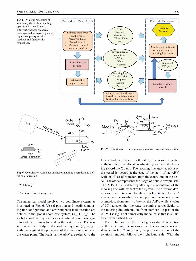
The flow chart of the proposed approach is illustrated in Fig. 5. The procedure consists of two main steps. First, the mean environmental loads, including wind, wave, cur-rent loads, and the mooring load are considered. The total resultant forces for the vessel in surge, sway and yaw are then obtained. By applying a reasonable thrust allocation scheme, the required thrust for each of the thrust units is acquired. These thrust forces serve as the static forces to balance the mean external loads on the vessel and keep the vessel in position. The initial heel and trim angles are also inherently captured. Thus, an initial equilibrium condition is achieved and dynamic simulation can be performed. Sec-ond, during the dynamic simulation, a simplified dynamic positioning system (proportional control) is used to repre-sent the manoeuvring of the master to maintain the vessel position. Then, sea-keeping analysis is performed to obtain the dynamic behaviour of the vessel and the mooring line. Compared to the “common practice approach”, more details on the dynamic behaviour of an AHV during AHO can be studied and analysed with the proposed procedure.

3 Theoretical background and numerical model

3.1 General

In this study, the numerical model was established in the SIMO and RIFLEX program package. SIMO [11] is a multi-body dynamic and time-domain program with emphasis on hydrodynamics and mechanical coupling between bodies. A SIMO body can have hydrodynamic properties based on potential theory. RIFLEX [12] is a pro-gram based on the finite element method (FEM) for model-ling slender marine structures like mooring lines and risers. Non-linearities and large deformations can be modelled. In a SIMO-RIFLEX coupled model, the SIMO bodies are attached to the RIFLEX elements. At each time step, the hydrodynamic loads and coupling forces are calculated inside SIMO and then transferred to RIFLEX. RIFLEX will then solve the equations of motion of the beam or bar elements and return the motion of the SIMO body. In this manner, the interaction between the body and the slender structures is computed.

In this section, a brief introduction about the theoretical background will be presented.

659J Mar Sci Technol (2017) 22:655–672

1 3

3.2 Theory

3.2.1 Coordination system

The numerical model involves two coordinate systems as illustrated in Fig.  6. Vessel position and heading, moor-ing line configuration and environmental load direction are defined in the global coordinate system, (XG, YG, ZG). The global coordinate system is an earth-fixed coordinate sys-tem and the origin is located on the water plane. The ves-sel has its own body-fixed coordinate system, (xB, yB, zB), with the origin at the projection of the centre of gravity on the water plane. The loads on the AHV are referred to the

local coordinate system. In this study, the vessel is located at the origin of the global coordinate system with the head-ing toward the XG axis. The mooring line attached point on the vessel is located at the edge of the stern of the AHV, with an off-set of m meters from the centre line of the ves-sel. The off-set represents the usage of double tow pin sets. The AOA, �, is modeled by altering the orientation of the mooring line with respect to the xB axis. The direction defi-nitions of wave (�) are also shown in Fig. 6. A value of 0◦ means that the weather is coming along the mooring line orientation, from stern to bow of the AHV, while a value of 90◦ indicates that the wave is coming perpendicular to the mooring line orientation, from starboard to port of the AHV. The rig is not numerically modelled so that it is illus-trated with dashed lines.

The definition of the six-degree-of-freedom motion of the vessel and the mooring line loads components are sketched in Fig. 7. As shown, the position direction of the rotational motion follows the right-hand rule. With the

Fig. 5 Analysis procedure of simulating the anchor handling operation in time domain. The oval, rounded rectangle, rectangle and hexagon represent inputs, temporary results, methods and final results, respectively

Estimation of Mean Loads

Environmentalconditions:- Wind- Wave- Current

VesselProperties

- Geometry- Thrust Units

etc.

Mooring line Configuration

- Property- Length- Angles

Estimate mean loadson the vessel:

- Mean wind load- Mean drift load- Mean current load- Mooring line load

Thrust allocation method

Estimate the required thrust

Dynamic Simulation

Set initial thrust of thrusters. Provide an initial condition for time domain simulation.

Sea-keeping analysis to obtain motions and

mooring line tension

Response Statistics

Coupled dynamic model

Simplified DP system

Rig

AHV

GlobalCoord.

Mooring Line

ψWave

LocalCoord.

xB

yB

oB β m

90°180°

270°

0°

OG XG

YG

Fig. 6 Coordinate systems for an anchor handling operation and defi-nition of direction

AHVoB

zBxByB

T

Th Ty

Tx

Tz

Mooring Line

m Surge

Sway

RollPitch

HeaveYaw

Fig. 7 Definition of vessel motion and mooring loads decomposition

660 J Mar Sci Technol (2017) 22:655–672

1 3

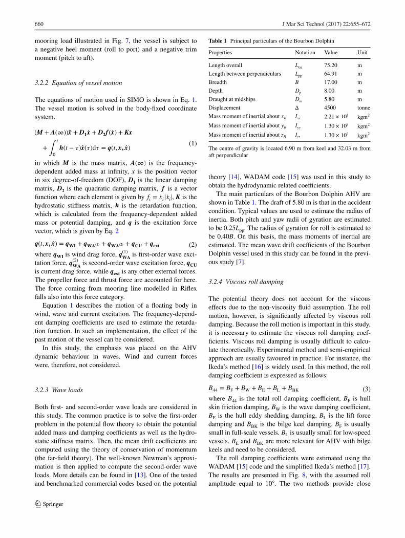
mooring load illustrated in Fig. 7, the vessel is subject to a negative heel moment (roll to port) and a negative trim moment (pitch to aft).

3.2.2 Equation of vessel motion

The equations of motion used in SIMO is shown in Eq. 1. The vessel motion is solved in the body-fixed coordinate system.

in which M is the mass matrix, A(∞) is the frequency-dependent added mass at infinity, x is the position vector in six degree-of-freedom (DOF), D1 is the linear damping matrix, D2 is the quadratic damping matrix, f is a vector function where each element is given by fi = xi|xi|, K is the hydrostatic stiffness matrix, h is the retardation function, which is calculated from the frequency-dependent added mass or potential damping, and q is the excitation force vector, which is given by Eq. 2

where q�� is wind drag force, q(1)��

is first-order wave exci-tation force, q(2)

�� is second-order wave excitation force, q��

is current drag force, while q��� is any other external forces. The propeller force and thrust force are accounted for here. The force coming from mooring line modelled in Riflex falls also into this force category.

Equation  1 describes the motion of a floating body in wind, wave and current excitation. The frequency-depend-ent damping coefficients are used to estimate the retarda-tion function. In such an implementation, the effect of the past motion of the vessel can be considered.

In this study, the emphasis was placed on the AHV dynamic behaviour in waves. Wind and current forces were, therefore, not considered.

3.2.3 Wave loads

Both first- and second-order wave loads are considered in this study. The common practice is to solve the first-order problem in the potential flow theory to obtain the potential added mass and damping coefficients as well as the hydro-static stiffness matrix. Then, the mean drift coefficients are computed using the theory of conservation of momentum (the far-field theory). The well-known Newman’s approxi-mation is then applied to compute the second-order wave loads. More details can be found in [13]. One of the tested and benchmarked commercial codes based on the potential

(1)(M + A(∞))x + D1x + D2f (x) + Kx

+ ∫t

0

h(t − �)x(�)d� = q(t, x, x)

(2)q(t, x, x) = q�� + q��(�) + q��(�) + q�� + q���

theory [14], WADAM code [15] was used in this study to obtain the hydrodynamic related coefficients.

The main particulars of the Bourbon Dolphin AHV are shown in Table 1. The draft of 5.80 m is that in the accident condition. Typical values are used to estimate the radius of inertia. Both pitch and yaw radii of gyration are estimated to be 0.25Lpp. The radius of gyration for roll is estimated to be 0.40B. On this basis, the mass moments of inertial are estimated. The mean wave drift coefficients of the Bourbon Dolphin vessel used in this study can be found in the previ-ous study [7].

3.2.4 Viscous roll damping

The potential theory does not account for the viscous effects due to the non-viscosity fluid assumption. The roll motion, however, is significantly affected by viscous roll damping. Because the roll motion is important in this study, it is necessary to estimate the viscous roll damping coef-ficients. Viscous roll damping is usually difficult to calcu-late theoretically. Experimental method and semi-empirical approach are usually favoured in practice. For instance, the Ikeda’s method [16] is widely used. In this method, the roll damping coefficient is expressed as follows:

where B44 is the total roll damping coefficient, BF is hull skin friction damping, BW is the wave damping coefficient, BE is the hull eddy shedding damping, BL is the lift force damping and BBK is the bilge keel damping. BF is usually small in full-scale vessels. BL is usually small for low-speed vessels. BE and BBK are more relevant for AHV with bilge keels and need to be considered.

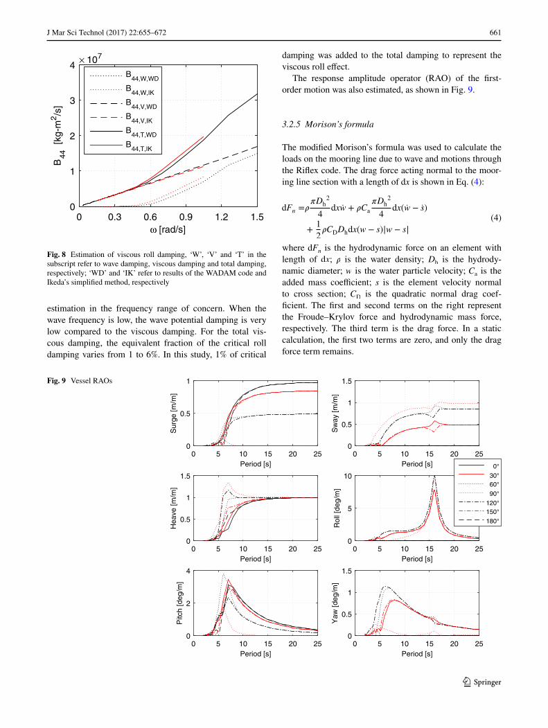
The roll damping coefficients were estimated using the WADAM [15] code and the simplified Ikeda’s method [17]. The results are presented in Fig. 8, with the assumed roll amplitude equal to 10◦. The two methods provide close

(3)B44 = BF + BW + BE + BL + BBK

Table 1 Principal particulars of the Bourbon Dolphin

The centre of gravity is located 6.90 m from keel and 32.03 m from aft perpendicular

Properties Notation Value Unit

Length overall Loa 75.20 mLength between perpendiculars Lpp 64.91 mBreadth B 17.00 mDepth Dp 8.00 mDraught at midships Dm 5.80 mDisplacement Δ 4500 tonneMass moment of inertial about xB Ixx 2.21 × 108 kgm2

Mass moment of inertial about yB Iyy 1.30 × 109 kgm2

Mass moment of inertial about zB Izz 1.30 × 109 kgm2

661J Mar Sci Technol (2017) 22:655–672

1 3

estimation in the frequency range of concern. When the wave frequency is low, the wave potential damping is very low compared to the viscous damping. For the total vis-cous damping, the equivalent fraction of the critical roll damping varies from 1 to 6%. In this study, 1% of critical

damping was added to the total damping to represent the viscous roll effect.

The response amplitude operator (RAO) of the first-order motion was also estimated, as shown in Fig. 9.

3.2.5 Morison’s formula

The modified Morison’s formula was used to calculate the loads on the mooring line due to wave and motions through the Riflex code. The drag force acting normal to the moor-ing line section with a length of dx is shown in Eq. (4):

where dFn is the hydrodynamic force on an element with length of dx; � is the water density; Dh is the hydrody-namic diameter; w is the water particle velocity; Ca is the added mass coefficient; s is the element velocity normal to cross section; CD is the quadratic normal drag coef-ficient. The first and second terms on the right represent the Froude–Krylov force and hydrodynamic mass force, respectively. The third term is the drag force. In a static calculation, the first two terms are zero, and only the drag force term remains.

(4)dFn =𝜌

𝜋Dh2

4dxw + 𝜌Ca

𝜋Dh2

4dx(w − s)

+1

2𝜌CDDhdx(w − s)|w − s|ω [rad/s]

0 0.3 0.6 0.9 1.2 1.5

B44

[kg

-m2/s

]× 107

0

1

2

3

4B

44,W,WD

B44,W,IK

B44,V,WD

B44,V,IK

B44,T,WD

B44,T,IK

Fig. 8 Estimation of viscous roll damping, ‘W’, ‘V’ and ‘T’ in the subscript refer to wave damping, viscous damping and total damping, respectively; ‘WD’ and ‘IK’ refer to results of the WADAM code and Ikeda’s simplified method, respectively

Fig. 9 Vessel RAOs

Period [s]0 5 10 15 20 25

Sur

ge [m

/m]

0

0.5

1

Period [s]0 5 10 15 20 25

Sw

ay [m

/m]

0

0.5

1

1.5

Period [s]0 5 10 15 20 25

Hea

ve [m

/m]

0

0.5

1

1.5

Period [s]0 5 10 15 20 25

Rol

l [de

g/m

]

0

5

10

Period [s]0 5 10 15 20 25

Pitc

h [d

eg/m

]

0

2

4

Period [s]0 5 10 15 20 25

Yaw

[deg

/m]

0

0.5

1

1.5

0°

30° 60°

90°

120°150°

180°

662 J Mar Sci Technol (2017) 22:655–672

1 3

3.2.6 Dynamic FE formulation

The mooring line is modelled as beam elements in an finite element (FE) framework in this study. A general expression of the spatial discretized FE system in dynamic equilibrium is shown in Eq. (5).

where RI, RD and RS are the inertia force vector, damp-ing force vector and internal structural reaction force vec-tor, respectively; r, r and r are the structural displacement, velocity and acceleration vectors, respectively. More details can be found in [12].

3.2.7 Thrust allocation

In this study, the thrust allocation approach is based on [18]. The general relation between the control demand and the individual actuator demand thrusts is shown in Eq. (6):

where �� is the vector of thrust and moment demand from the controller, T�� is a vector of thruster demands in Carte-sian coordinates, and T� is the thruster allocation matrix, defined as follows:

and

where n is the number of thrusters. In our case, only hori-zontal plane motions, i.e., surge, sway and yaw are to be balanced, the matrices ti in Eq. (8) are given by Eq. (9):

where lix and liy are the longitudinal and transverse posi-tions of the ith thruster, respectively. In general, there will be more variables describing the thruster settings than the equations to solve. This is usually formulated as an opti-mization problem, introducing an power minimization con-dition. According to [19], using the least-norm solution of T�� can be achieved by finding the Moore–Penrose gener-alized inverse of Ta. The solution can be expressed in the following form:

(5)RI(r, r,t) + RD(r, r,t) + RS(r,t) = RE(r, r,t)

(6)�c = T�T��

(7)T�� = [T1x T1y … Tnx Tny]

(8)T� = [t1 … tn]

(9)

ti =

⎡⎢⎢⎣

1 0

0 1

−liy lix

⎤⎥⎥⎦

⏟⏞⏟⏞⏟

azimuth

thruster

, ti =

⎡⎢⎢⎣

1 0

0 0

−liy 0

⎤⎥⎥⎦

⏟⏟⏟

main

propeller

, ti =

⎡⎢⎢⎣

0 0

0 1

0 lix

⎤⎥⎥⎦

⏟⏟⏟

tunnel

thruster

(10)T�� = T†

���

(11)T†

𝐚= W−1TT

𝐚(TaW

−1TaT)−1

where T†

� is the generalised inverse of T�, W is weighting

matrix.When the required thrust, i.e., T�� is obtained by Eq.

(10), it is set as a constant value in the vessel model to represent the initial forces to balance the static mean external loads.

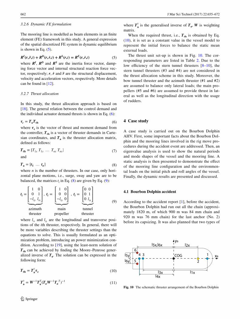
The thrust unit set-up is shown in Fig.  10. The cor-responding parameters are listed in Table  2. Due to the low efficiency of the stern tunnel thrusters [8–10], the stern tunnel thrusters (#3 and #4) are not considered in the thrust allocation scheme in this study. Moreover, the bow tunnel thruster and the azimuth thruster (#1 and #2) are assumed to balance only lateral loads; the main pro-pellers (#5 and #6) are assumed to provide thrust in lat-eral as well as the longitudinal direction with the usage of rudders.

4 Case study

A case study is carried out on the Bourbon Dolphin AHV. First, some important facts about the Bourbon Dol-phin and the mooring lines involved in the rig move pro-cedures during the accident event are addressed. Then, an eigenvalue analysis is used to show the natural periods and mode shapes of the vessel and the mooring line. A static analysis is then presented to demonstrate the effect of the mooring line configuration and the environmen-tal loads on the initial pitch and roll angles of the vessel. Finally, the dynamic results are presented and discussed.

4.1 Bourbon Dolphin accident

According to the accident report [1], before the accident, the Bourbon Dolphin had run out all the chain (approxi-mately 1820 m, of which 900 m was 84 mm chain and 920 m was 76 mm chain) for the last anchor (No. 2) before its capsizing. It was also planned that two types of

COG

l2x

l1xl4x

l3x

l5x,l6x

l5yl6y

1

2

34

5

6xB

yB

Fig. 10 The schematic thruster arrangement of the Bourbon Dolphin

663J Mar Sci Technol (2017) 22:655–672

1 3

work wire would be used in the anchor deployment pro-cedure. The relevant mooring line properties are listed in Table  3. At the moment of capsizing, the vertical angle (the angle between the mooring line and the vertical plane, see Fig. 3, was 38◦.

4.2 Eigenvalue analysis

The purpose of an eigenvalue analysis is to identify the natu-ral periods and eigenmodes of a dynamic system, by solving the following equation in the frequency domain.

in which � is the eigenvalue, M is the mass matrix, A(�) is the frequency-dependent added mass matrix, K is the stiff-ness matrix, � is the eigenvector. The natural period Ti of the system for eigenvector Φi is given by Eq. (13).

(12)[−�(M + A(�)) + K]� = 0

(13)Ti =2�√�i

4.2.1 Vessel alone

The eigenvectors and natural periods of the vessel alone are first calculated. The natural periods of the horizon-tal plane motions were set to 120 s by adjusting the cor-responding proportional gain in the DP system. For this case in Eq. (12), M represents the vessel mass matrix, A(�) is the added mass at infinite frequency (A(∞)), K consists of the linear hydrostatic stiffness in the vertical plane and the stiffness (proportional gain) from the DP system in the horizontal plane. The results are presented in Table  4 and the dominant motion components are emphasised in bold style. As shown, the first three modes are dominated by the motions in the horizontal plane, with a natural period approximately at 120 s. The sway motion is coupled with the yaw motion in mode 3 to a certain extend. Modes 4, 5 and 6 represent the vertical motions. The natural periods for roll (mode 4) and pitch (mode 6) are 15.37 and 5.41 s, respectively. In mode 5, the heave motion is coupled with the pitch motion and thus there is no pure heave mode.

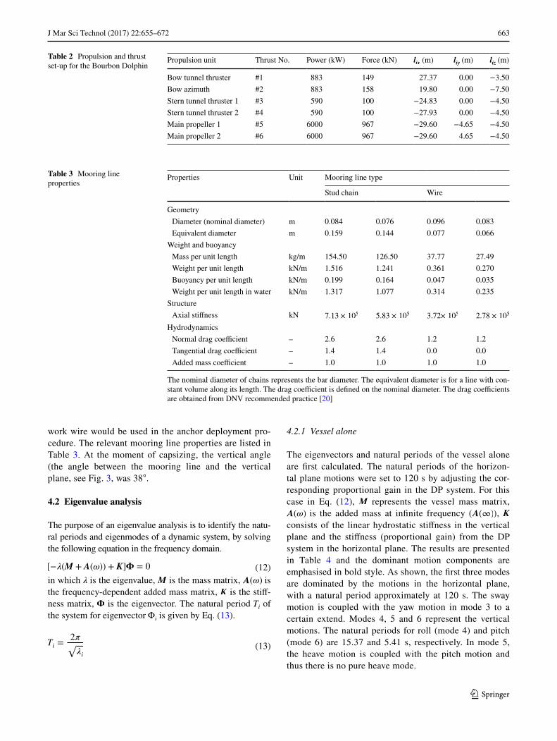
Table 2 Propulsion and thrust set-up for the Bourbon Dolphin

Propulsion unit Thrust No. Power (kW) Force (kN) lix (m) liy (m) liz (m)

Bow tunnel thruster #1 883 149 27.37 0.00 −3.50Bow azimuth #2 883 158 19.80 0.00 −7.50Stern tunnel thruster 1 #3 590 100 −24.83 0.00 −4.50Stern tunnel thruster 2 #4 590 100 −27.93 0.00 −4.50Main propeller 1 #5 6000 967 −29.60 −4.65 −4.50Main propeller 2 #6 6000 967 −29.60 4.65 −4.50

Table 3 Mooring line properties

The nominal diameter of chains represents the bar diameter. The equivalent diameter is for a line with con-stant volume along its length. The drag coefficient is defined on the nominal diameter. The drag coefficients are obtained from DNV recommended practice [20]

Properties Unit Mooring line type

Stud chain Wire

Geometry Diameter (nominal diameter) m 0.084 0.076 0.096 0.083 Equivalent diameter m 0.159 0.144 0.077 0.066

Weight and buoyancy Mass per unit length kg/m 154.50 126.50 37.77 27.49 Weight per unit length kN/m 1.516 1.241 0.361 0.270 Buoyancy per unit length kN/m 0.199 0.164 0.047 0.035 Weight per unit length in water kN/m 1.317 1.077 0.314 0.235

Structure Axial stiffness kN 7.13 × 105 5.83 × 105 3.72× 105 2.78 × 105

Hydrodynamics Normal drag coefficient – 2.6 2.6 1.2 1.2 Tangential drag coefficient – 1.4 1.4 0.0 0.0 Added mass coefficient – 1.0 1.0 1.0 1.0

664 J Mar Sci Technol (2017) 22:655–672

1 3

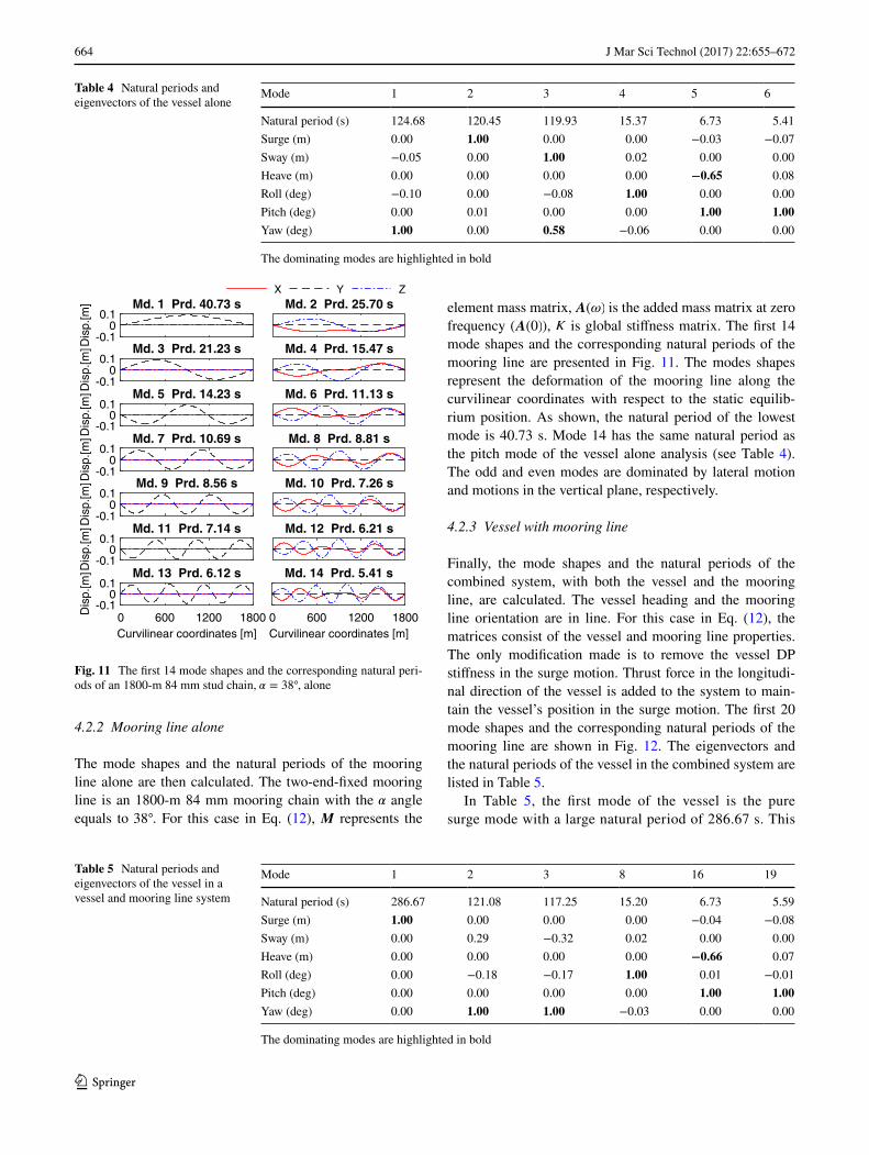
4.2.2 Mooring line alone

The mode shapes and the natural periods of the mooring line alone are then calculated. The two-end-fixed mooring line is an 1800-m 84 mm mooring chain with the � angle equals to 38◦. For this case in Eq. (12), M represents the

element mass matrix, A(�) is the added mass matrix at zero frequency (A(0)), K is global stiffness matrix. The first 14 mode shapes and the corresponding natural periods of the mooring line are presented in Fig.  11. The modes shapes represent the deformation of the mooring line along the curvilinear coordinates with respect to the static equilib-rium position. As shown, the natural period of the lowest mode is 40.73 s. Mode 14 has the same natural period as the pitch mode of the vessel alone analysis (see Table 4). The odd and even modes are dominated by lateral motion and motions in the vertical plane, respectively.

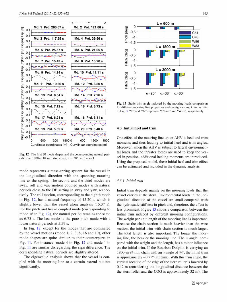
4.2.3 Vessel with mooring line

Finally, the mode shapes and the natural periods of the combined system, with both the vessel and the mooring line, are calculated. The vessel heading and the mooring line orientation are in line. For this case in Eq. (12), the matrices consist of the vessel and mooring line properties. The only modification made is to remove the vessel DP stiffness in the surge motion. Thrust force in the longitudi-nal direction of the vessel is added to the system to main-tain the vessel’s position in the surge motion. The first 20 mode shapes and the corresponding natural periods of the mooring line are shown in Fig.  12. The eigenvectors and the natural periods of the vessel in the combined system are listed in Table 5.

In Table  5, the first mode of the vessel is the pure surge mode with a large natural period of 286.67 s. This

Table 4 Natural periods and eigenvectors of the vessel alone

The dominating modes are highlighted in bold

Mode 1 2 3 4 5 6

Natural period (s) 124.68 120.45 119.93 15.37 6.73 5.41Surge (m) 0.00 1.00 0.00 0.00 −0.03 −0.07Sway (m) −0.05 0.00 1.00 0.02 0.00 0.00Heave (m) 0.00 0.00 0.00 0.00 −0.65 0.08Roll (deg) −0.10 0.00 −0.08 1.00 0.00 0.00Pitch (deg) 0.00 0.01 0.00 0.00 1.00 1.00Yaw (deg) 1.00 0.00 0.58 −0.06 0.00 0.00

Dis

p.[m

]

-0.10

0.1Md. 1 Prd. 40.73 s Md. 2 Prd. 25.70 s

Dis

p.[m

]

-0.10

0.1Md. 3 Prd. 21.23 s Md. 4 Prd. 15.47 s

Dis

p.[m

]

-0.10

0.1Md. 5 Prd. 14.23 s Md. 6 Prd. 11.13 s

Dis

p.[m

]

-0.10

0.1Md. 7 Prd. 10.69 s Md. 8 Prd. 8.81 s

Dis

p.[m

]

-0.10

0.1Md. 9 Prd. 8.56 s Md. 10 Prd. 7.26 s

Dis

p.[m

]

-0.10

0.1Md. 11 Prd. 7.14 s Md. 12 Prd. 6.21 s

Curvilinear coordinates [m]0 600 1200 1800D

isp.

[m]

-0.10

0.1Md. 13 Prd. 6.12 s

Curvilinear coordinates [m]0 600 1200 1800

Md. 14 Prd. 5.41 s

X Y Z

Fig. 11 The first 14 mode shapes and the corresponding natural peri-ods of an 1800-m 84 mm stud chain, � = 38

◦, alone

Table 5 Natural periods and eigenvectors of the vessel in a vessel and mooring line system

The dominating modes are highlighted in bold

Mode 1 2 3 8 16 19

Natural period (s) 286.67 121.08 117.25 15.20 6.73 5.59Surge (m) 1.00 0.00 0.00 0.00 −0.04 −0.08Sway (m) 0.00 0.29 −0.32 0.02 0.00 0.00Heave (m) 0.00 0.00 0.00 0.00 −0.66 0.07Roll (deg) 0.00 −0.18 −0.17 1.00 0.01 −0.01Pitch (deg) 0.00 0.00 0.00 0.00 1.00 1.00Yaw (deg) 0.00 1.00 1.00 −0.03 0.00 0.00

665J Mar Sci Technol (2017) 22:655–672

1 3

mode represents a mass-spring system for the vessel in the longitudinal direction with the spanning mooring line as the spring. The second and the third modes are sway, roll and yaw motion coupled modes with natural periods close to the DP setting in sway and yaw, respec-tively. The roll motion, corresponding to the eighth mode in Fig. 12, has a natural frequency of 15.20 s, which is slightly lower than the vessel alone analysis (15.37 s). For the pitch and heave coupled mode (corresponding to mode 16 in Fig. 12), the natural period remains the same as 6.73 s. The last mode is the pure pitch mode with a lower natural periods at 5.59 s.

In Fig.  12, except for the modes that are dominated by the vessel motions (mode 1, 2, 3, 8, 16 and 19), other mode shapes are quite similar to their counterparts in Fig. 11. For instance, mode 4 in Fig. 12 and mode 1 in Fig. 11 are similar disregarding the sign difference. The corresponding natural periods are slightly altered.

The eigenvalue analysis shows that the vessel is cou-pled with the mooring line to a certain extend but not significantly.

4.3 Initial heel and trim

One effect of the mooring line on an AHV is heel and trim moments and thus leading to initial heel and trim angles. Moreover, when the AHV is subject to lateral environmen-tal loads and the thruster forces are used to keep the ves-sel in position, additional heeling moments are introduced. Using the proposed model, these initial heel and trim effect can be estimated and included in the dynamic analysis.

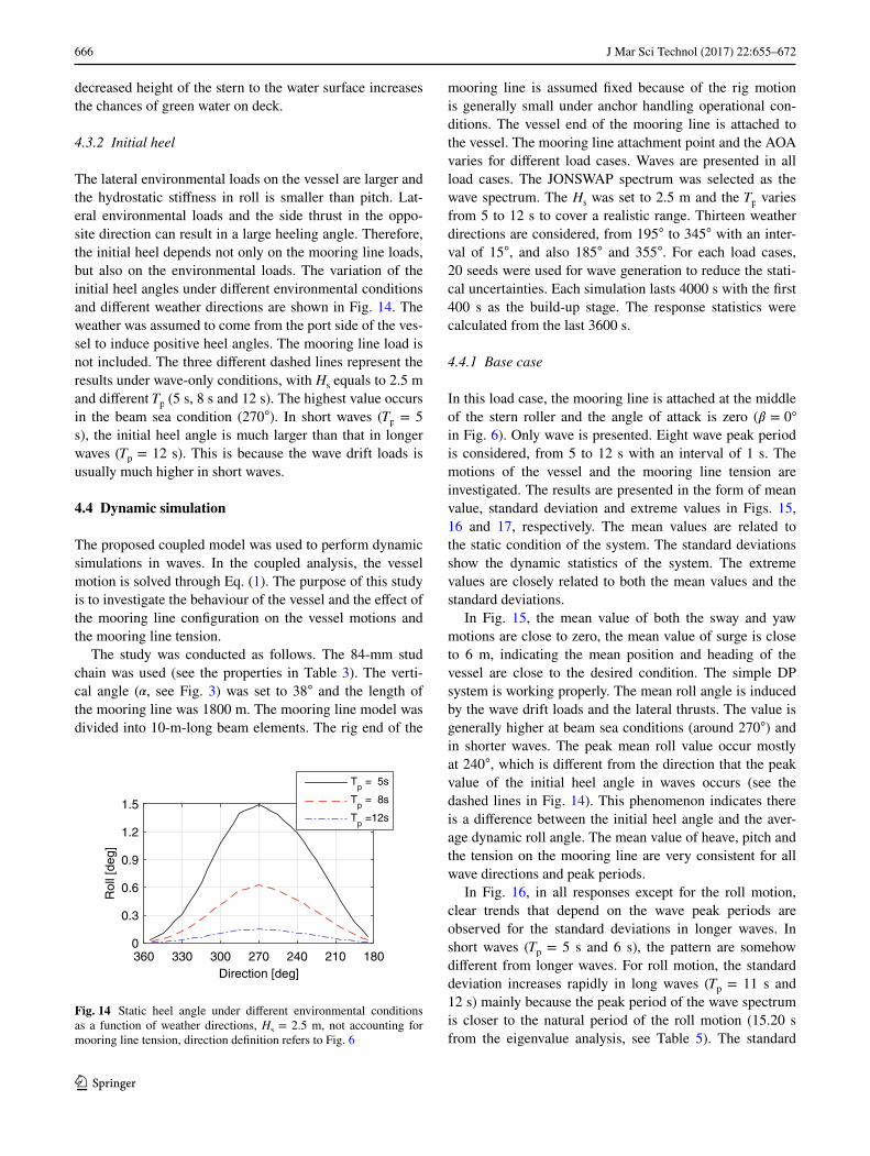
4.3.1 Initial trim

Initial trim depends mainly on the mooring loads that the vessel carries at the stern. Environmental loads in the lon-gitudinal direction of the vessel are small compared with the hydrostatic stiffness in pitch and, therefore, the effect is less prominent. Figure 13 shows a comparison between the initial trim induced by different mooring configurations. The weight per unit length of the mooring line is important. Because the chain section is much heavier than the wire section, the initial trim with chain section is much larger. The total length is also important. The longer the moor-ing line, the heavier the mooring line. The � angle, com-pared with the weight and the length, has a minor influence on the initial trim. If the Bourbon Dolphin is carrying an 1800-m 84 mm chain with an � angle of 38◦, the initial trim is approximately −0.75◦ (aft trim). With this trim angle, the vertical location of the edge of the stern roller is lowered by 0.42 m (considering the longitudinal distance between the the stern roller and the COG is approximately 32 m). The

Dis

p.[m

]

-0.10

0.1Md. 1 Prd. 286.67 s Md. 2 Prd. 121.08 s

Dis

p.[m

]

-0.10

0.1Md. 3 Prd. 117.25 s Md. 4 Prd. 39.56 s

Dis

p.[m

]

-0.10

0.1Md. 5 Prd. 25.57 s Md. 6 Prd. 21.05 s

Dis

p.[m

]

-0.10

0.1Md. 7 Prd. 15.43 s Md. 8 Prd. 15.20 s

Dis

p.[m

]

-0.10

0.1Md. 9 Prd. 14.14 s Md. 10 Prd. 11.11 s

Dis

p.[m

]

-0.10

0.1Md. 11 Prd. 10.66 s Md. 12 Prd. 8.80 s

Dis

p.[m

]

-0.10

0.1Md. 13 Prd. 8.54 s Md. 14 Prd. 7.26 s

Dis

p.[m

]

-0.10

0.1Md. 15 Prd. 7.12 s Md. 16 Prd. 6.73 s

Dis

p.[m

]

-0.10

0.1Md. 17 Prd. 6.21 s Md. 18 Prd. 6.11 s

Curvilinear coordinates [m]0 600 1200 1800D

isp.

[m]

-0.10

0.1Md. 19 Prd. 5.59 s

Curvilinear coordinates [m]0 600 1200 1800

Md. 20 Prd. 5.40 s

X Y Z

Fig. 12 The first 20 mode shapes and the corresponding natural peri-ods of an 1800-m 84 mm stud chain, � = 38

◦, with vessel

Pitc

h [d

eg]

-1.5

-1

-0.5

0L = 600 m

Pitc

h [d

eg]

-1.5

-1

-0.5

0L = 1800 m

α=20° α=38° α=60°

Pitc

h [d

eg]

-1.5

-1

-0.5

0L = 3000 m

C84C76W96W83

Fig. 13 Static trim angle induced by the mooring loads comparison for different mooring line properties and configurations; L and � refer to Fig. 3, “C” and “W” represent “Chain” and “Wire”, respectively

666 J Mar Sci Technol (2017) 22:655–672

1 3

decreased height of the stern to the water surface increases the chances of green water on deck.

4.3.2 Initial heel

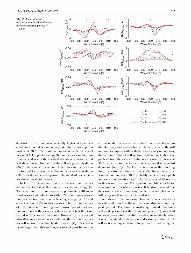
The lateral environmental loads on the vessel are larger and the hydrostatic stiffness in roll is smaller than pitch. Lat-eral environmental loads and the side thrust in the oppo-site direction can result in a large heeling angle. Therefore, the initial heel depends not only on the mooring line loads, but also on the environmental loads. The variation of the initial heel angles under different environmental conditions and different weather directions are shown in Fig. 14. The weather was assumed to come from the port side of the ves-sel to induce positive heel angles. The mooring line load is not included. The three different dashed lines represent the results under wave-only conditions, with Hs equals to 2.5 m and different Tp (5 s, 8 s and 12 s). The highest value occurs in the beam sea condition (270◦). In short waves (Tp = 5 s), the initial heel angle is much larger than that in longer waves (Tp = 12 s). This is because the wave drift loads is usually much higher in short waves.

4.4 Dynamic simulation

The proposed coupled model was used to perform dynamic simulations in waves. In the coupled analysis, the vessel motion is solved through Eq. (1). The purpose of this study is to investigate the behaviour of the vessel and the effect of the mooring line configuration on the vessel motions and the mooring line tension.

The study was conducted as follows. The 84-mm stud chain was used (see the properties in Table 3). The verti-cal angle (�, see Fig.  3) was set to 38◦ and the length of the mooring line was 1800 m. The mooring line model was divided into 10-m-long beam elements. The rig end of the

mooring line is assumed fixed because of the rig motion is generally small under anchor handling operational con-ditions. The vessel end of the mooring line is attached to the vessel. The mooring line attachment point and the AOA varies for different load cases. Waves are presented in all load cases. The JONSWAP spectrum was selected as the wave spectrum. The Hs was set to 2.5 m and the Tp varies from 5 to 12 s to cover a realistic range. Thirteen weather directions are considered, from 195◦ to 345◦ with an inter-val of 15◦, and also 185◦ and 355◦. For each load cases, 20 seeds were used for wave generation to reduce the stati-cal uncertainties. Each simulation lasts 4000 s with the first 400 s as the build-up stage. The response statistics were calculated from the last 3600 s.

4.4.1 Base case

In this load case, the mooring line is attached at the middle of the stern roller and the angle of attack is zero (� = 0◦ in Fig. 6). Only wave is presented. Eight wave peak period is considered, from 5 to 12 s with an interval of 1 s. The motions of the vessel and the mooring line tension are investigated. The results are presented in the form of mean value, standard deviation and extreme values in Figs.  15, 16 and 17, respectively. The mean values are related to the static condition of the system. The standard deviations show the dynamic statistics of the system. The extreme values are closely related to both the mean values and the standard deviations.

In Fig.  15, the mean value of both the sway and yaw motions are close to zero, the mean value of surge is close to 6 m, indicating the mean position and heading of the vessel are close to the desired condition. The simple DP system is working properly. The mean roll angle is induced by the wave drift loads and the lateral thrusts. The value is generally higher at beam sea conditions (around 270◦) and in shorter waves. The peak mean roll value occur mostly at 240◦, which is different from the direction that the peak value of the initial heel angle in waves occurs (see the dashed lines in Fig. 14). This phenomenon indicates there is a difference between the initial heel angle and the aver-age dynamic roll angle. The mean value of heave, pitch and the tension on the mooring line are very consistent for all wave directions and peak periods.

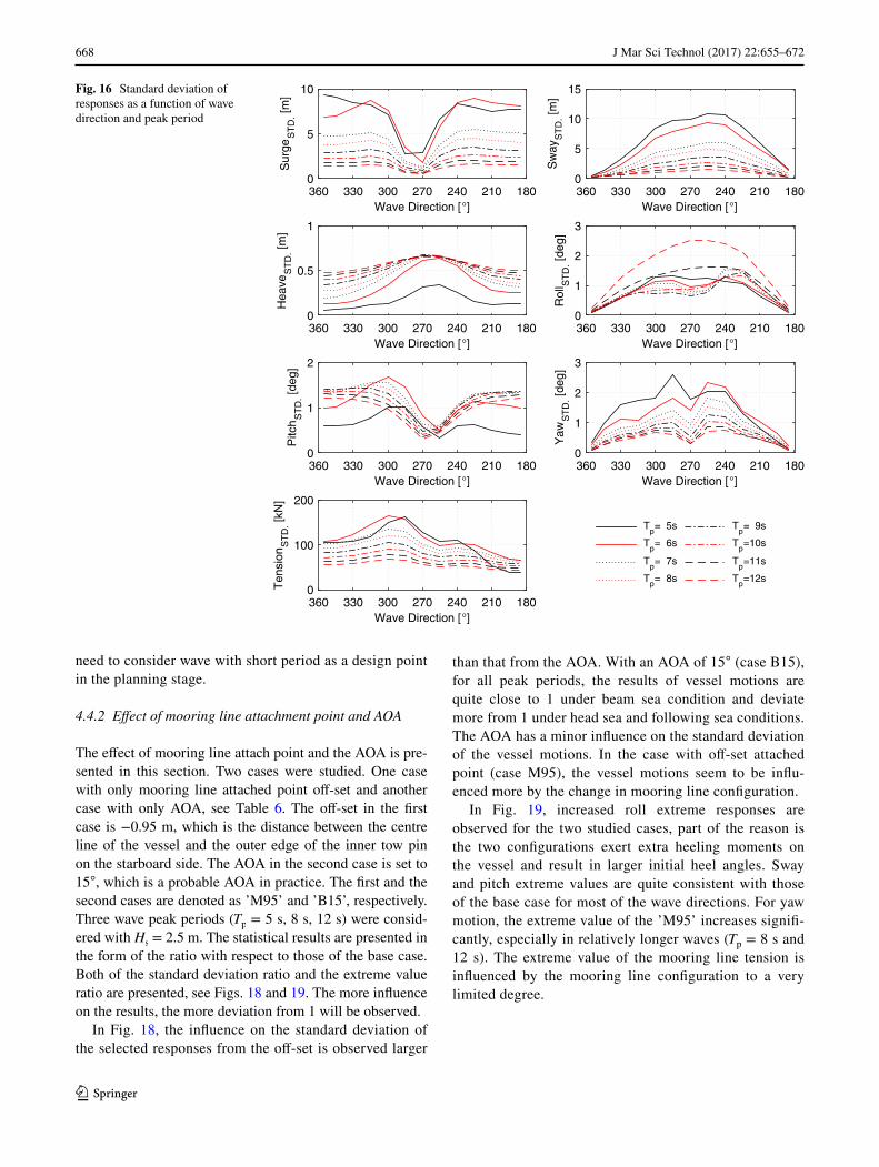
In Fig.  16, in all responses except for the roll motion, clear trends that depend on the wave peak periods are observed for the standard deviations in longer waves. In short waves (Tp = 5 s and 6 s), the pattern are somehow different from longer waves. For roll motion, the standard deviation increases rapidly in long waves (Tp = 11 s and 12 s) mainly because the peak period of the wave spectrum is closer to the natural period of the roll motion (15.20 s from the eigenvalue analysis, see Table  5). The standard

Direction [deg]180210240270300330360

Rol

l [de

g]

0

0.3

0.6

0.9

1.2

1.5

Tp = 5s

Tp = 8s

Tp =12s

Fig. 14 Static heel angle under different environmental conditions as a function of weather directions, H

s = 2.5 m, not accounting for

mooring line tension, direction definition refers to Fig. 6

667J Mar Sci Technol (2017) 22:655–672

1 3

deviation of roll motion is generally higher at beam sea conditions. For pitch motion the peak value occurs approxi-mately at 300◦. The result is consistent with the vessel motion RAO of pitch (see Fig. 9). For the mooring line ten-sion, dependence of the standard deviation on wave period and direction is observed. In the following sea condition (360◦), the standard deviation of the mooring line tension is observed to be larger than that in the head sea condition (180◦) for the same wave period. The standard deviation is also higher in shorter waves.

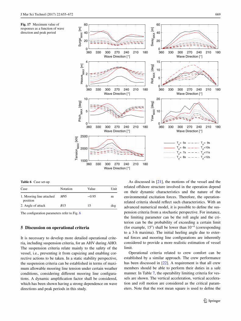
In Fig. 17, the general trends of the maximum values are similar to that of the standard deviations in Fig.  16. The maximum drift in sway is approximately 40 m in short waves and reduced to within 20 m in longer waves. For yaw motion, the maxim heading change is 15◦ and occurs around 255◦ in short waves. The extreme values of roll, pitch and mooring line tension are of concern. For roll motion the extreme values occur when the wave period is 12 s for all directions. However, it is observed also that under beam sea condition, the extreme values for roll motion in relatively short waves (Tp = 5 s and 6 s) are larger than that in longer waves. A possible reason

is that in shorter waves, wave drift forces are higher so that the sway and yaw motion are larger; because the roll motion is coupled with both the sway and yaw motions, the extreme value of roll motion is therefore higher. For pitch motion, the extreme value occurs when Tp is 6 s at 300◦, which is similar to the trends observed in standard deviation (see Fig.  16). For the tension in the mooring line, the extreme values are generally higher when the wave is coming from 300◦ probably because large pitch motion in combination with relatively large drift occurs in this wave direction. The dynamic amplification factor is as high as 1.55 when Tp is 6 s. It is also observed that the extreme value of mooring line tension is higher in the following sea than that in the head sea.

As shown, the mooring line tension characteris-tics depend significantly on the wave direction and the peak period. Therefore, considering limited directions and peak periods (in the “common practice”) may lead to non-conservative results. Besides, in relatively short waves, the standard deviation and extreme value of the roll motion is higher than in longer waves, indicating the

Fig. 15 Mean value of responses as a function of wave direction and peak period, H

s

= 2.5 m

Wave Direction [°]180210240270300330360

Sur

geM

EA

N [m

]

4

6

8

Wave Direction [°]180210240270300330360

Sw

ayM

EA

N [m

]

-2

-1

0

1

Wave Direction [°]180210240270300330360

Hea

veM

EA

N [m

]

-0.05

-0.045

-0.04

Wave Direction [°]180210240270300330360

Rol

l ME

AN

[deg

]

-1

0

1

2

Wave Direction [°]180210240270300330360

Pitc

hM

EA

N [d

eg]

-0.76

-0.75

-0.74

Wave Direction [°]180210240270300330360

Yaw

ME

AN

[deg

]

-2

-1

0

1

Wave Direction [°]180210240270300330360

Ten

sion

ME

AN

[kN

]

1500

1505

1510

Tp= 5s

Tp= 6s

Tp= 7s

Tp= 8s

Tp= 9s

Tp=10s

Tp=11s

Tp=12s

668 J Mar Sci Technol (2017) 22:655–672

1 3

need to consider wave with short period as a design point in the planning stage.

4.4.2 Effect of mooring line attachment point and AOA

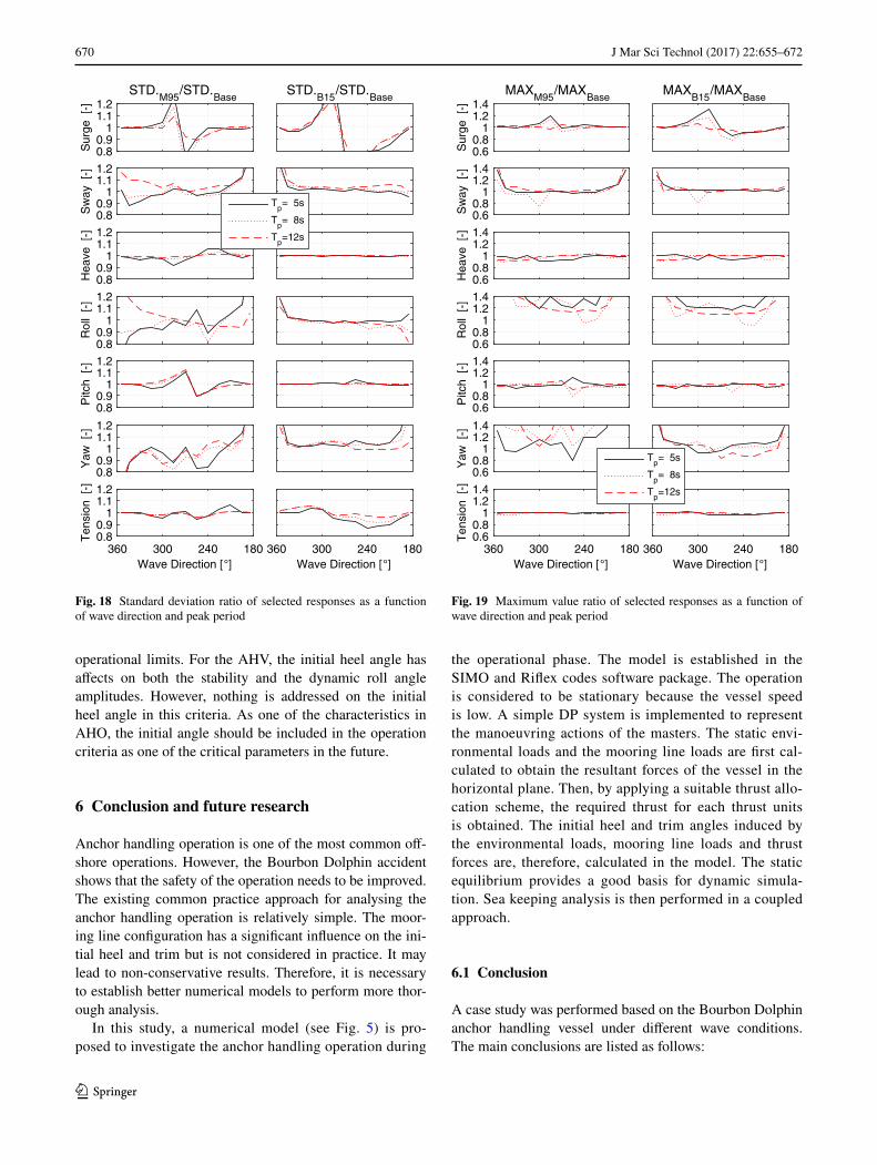
The effect of mooring line attach point and the AOA is pre-sented in this section. Two cases were studied. One case with only mooring line attached point off-set and another case with only AOA, see Table  6. The off-set in the first case is −0.95 m, which is the distance between the centre line of the vessel and the outer edge of the inner tow pin on the starboard side. The AOA in the second case is set to 15◦, which is a probable AOA in practice. The first and the second cases are denoted as ’M95’ and ’B15’, respectively. Three wave peak periods (Tp = 5 s, 8 s, 12 s) were consid-ered with Hs = 2.5 m. The statistical results are presented in the form of the ratio with respect to those of the base case. Both of the standard deviation ratio and the extreme value ratio are presented, see Figs. 18 and 19. The more influence on the results, the more deviation from 1 will be observed.

In Fig.  18, the influence on the standard deviation of the selected responses from the off-set is observed larger

than that from the AOA. With an AOA of 15◦ (case B15), for all peak periods, the results of vessel motions are quite close to 1 under beam sea condition and deviate more from 1 under head sea and following sea conditions. The AOA has a minor influence on the standard deviation of the vessel motions. In the case with off-set attached point (case M95), the vessel motions seem to be influ-enced more by the change in mooring line configuration.

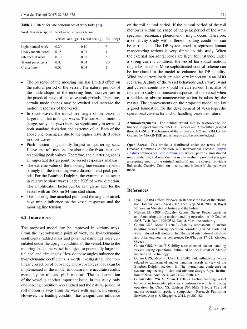
In Fig.  19, increased roll extreme responses are observed for the two studied cases, part of the reason is the two configurations exert extra heeling moments on the vessel and result in larger initial heel angles. Sway and pitch extreme values are quite consistent with those of the base case for most of the wave directions. For yaw motion, the extreme value of the ’M95’ increases signifi-cantly, especially in relatively longer waves (Tp = 8 s and 12 s). The extreme value of the mooring line tension is influenced by the mooring line configuration to a very limited degree.

Fig. 16 Standard deviation of responses as a function of wave direction and peak period

Wave Direction [°]180210240270300330360

Sur

geS

TD

. [m]

0

5

10

Wave Direction [°]180210240270300330360

Sw

ayS

TD

. [m]

0

5

10

15

Wave Direction [°]180210240270300330360

Hea

veS

TD

. [m]

0

0.5

1

Wave Direction [°]180210240270300330360

Rol

l ST

D. [d

eg]

0

1

2

3

Wave Direction [°]180210240270300330360

Pitc

hS

TD

. [deg

]

0

1

2

Wave Direction [°]180210240270300330360

Yaw

ST

D. [d

eg]

0

1

2

3

Wave Direction [°]180210240270300330360

Ten

sion

ST

D. [k

N]

0

100

200

Tp= 5s

Tp= 6s

Tp= 7s

Tp= 8s

Tp= 9s

Tp=10s

Tp=11s

Tp=12s

669J Mar Sci Technol (2017) 22:655–672

1 3

5 Discussion on operational criteria

It is necessary to develop more detailed operational crite-ria, including suspension criteria, for an AHV during AHO. The suspension criteria relate mainly to the safety of the vessel, i.e., preventing it from capsizing and enabling cor-rective actions to be taken. In a static stability perspective, the suspension criteria can be established in terms of maxi-mum allowable mooring line tension under certain weather conditions, considering different mooring line configura-tions. A dynamic amplification factor shall be considered, which has been shown having a strong dependence on wave directions and peak periods in this study.

As discussed in [21], the motions of the vessel and the related offshore structure involved in the operation depend on their dynamic characteristics and the nature of the environmental excitation forces. Therefore, the operation-related criteria should reflect such characteristics. With an advanced numerical model, it is possible to define the sus-pension criteria from a stochastic perspective. For instance, the limiting parameter can be the roll angle and the cri-terion can be the probability of exceeding a certain limit (for example, 15◦) shall be lower than 10−4 (corresponding to a 3-h maxima). The initial heeling angle due to exter-nal forces and mooring line configurations are inherently considered to provide a more realistic estimation of vessel limit.

Operational criteria related to crew comfort can be established by a similar approach. The crew performance has been discussed in [22]. A requirement is that all crew members should be able to perform their duties in a safe manner. In Table 7, the operability limiting criteria for ves-sels are shown. The vertical acceleration, vertical accelera-tion and roll motion are considered as the critical param-eters. Note that the root mean square is used to define the

Fig. 17 Maximum value of responses as a function of wave direction and peak period

Wave Direction [°]180210240270300330360

Sur

geM

AX

[m]

0

20

40

60

Wave Direction [°]180210240270300330360

Sw

ayM

AX

[m]

0

20

40

60

Wave Direction [°]180210240270300330360

Hea

veM

AX

[m]

0

2

4

Wave Direction [°]180210240270300330360

Rol

l MA

X [d

eg]

0

5

10

15

Wave Direction [°]180210240270300330360

Pitc

hM

AX

[deg

]

0

5

10

Wave Direction [°]180210240270300330360

Yaw

MA

X [d

eg]

0

10

20

Wave Direction [°]180210240270300330360

Ten

sion

MA

X [k

N]

1500

2000

2500

Tp= 5s

Tp= 6s

Tp= 7s

Tp= 8s

Tp= 9s

Tp=10s

Tp=11s

Tp=12s

Table 6 Case set-up

The configuration parameters refer to Fig. 6

Case Notation Value Unit

1. Mooring line attached position

M95 −0.95 m

2. Angle of attack B15 15 deg

670 J Mar Sci Technol (2017) 22:655–672

1 3

operational limits. For the AHV, the initial heel angle has affects on both the stability and the dynamic roll angle amplitudes. However, nothing is addressed on the initial heel angle in this criteria. As one of the characteristics in AHO, the initial angle should be included in the operation criteria as one of the critical parameters in the future.

6 Conclusion and future research

Anchor handling operation is one of the most common off-shore operations. However, the Bourbon Dolphin accident shows that the safety of the operation needs to be improved. The existing common practice approach for analysing the anchor handling operation is relatively simple. The moor-ing line configuration has a significant influence on the ini-tial heel and trim but is not considered in practice. It may lead to non-conservative results. Therefore, it is necessary to establish better numerical models to perform more thor-ough analysis.

In this study, a numerical model (see Fig.  5) is pro-posed to investigate the anchor handling operation during

the operational phase. The model is established in the SIMO and Riflex codes software package. The operation is considered to be stationary because the vessel speed is low. A simple DP system is implemented to represent the manoeuvring actions of the masters. The static envi-ronmental loads and the mooring line loads are first cal-culated to obtain the resultant forces of the vessel in the horizontal plane. Then, by applying a suitable thrust allo-cation scheme, the required thrust for each thrust units is obtained. The initial heel and trim angles induced by the environmental loads, mooring line loads and thrust forces are, therefore, calculated in the model. The static equilibrium provides a good basis for dynamic simula-tion. Sea keeping analysis is then performed in a coupled approach.

6.1 Conclusion

A case study was performed based on the Bourbon Dolphin anchor handling vessel under different wave conditions. The main conclusions are listed as follows:

Sur

ge [

-]

0.80.9

11.11.2

Sw

ay [

-]

0.80.9

11.11.2

Hea

ve [

-]

0.80.9

11.11.2

Rol

l [-

]

0.80.9

11.11.2

Pitc

h [-

]

0.80.9

11.11.2

Yaw

[-]

0.80.9

11.11.2

Wave Direction [°]180240300360

Ten

sion

[-]

0.80.9

11.11.2

Wave Direction [°]180240300360

Tp= 5s

Tp= 8s

Tp=12s

STD.M95

/STD.Base

STD.B15

/STD.Base

Fig. 18 Standard deviation ratio of selected responses as a function of wave direction and peak period

Sur

ge [

-]

0.60.8

11.21.4

Sw

ay [

-]

0.60.8

11.21.4

Hea

ve [

-]

0.60.8

11.21.4

Rol

l [-

]

0.60.8

11.21.4

Pitc

h [-

]

0.60.8

11.21.4

Yaw

[-]

0.60.8

11.21.4

Wave Direction [°]180240300360

Ten

sion

[-]

0.60.8

11.21.4

Wave Direction [°]180240300360

Tp= 5s

Tp= 8s

Tp=12s

MAXM95

/MAXBase

MAXB15

/MAXBase

Fig. 19 Maximum value ratio of selected responses as a function of wave direction and peak period

671J Mar Sci Technol (2017) 22:655–672

1 3

• The presence of the mooring line has limited effect on the natural period of the vessel. The natural periods of the mode shapes of the mooring line, however, are in the practical range of the wave peak periods. Therefore, certain mode shapes may be excited and increase the motion responses of the vessel.

• In short waves, the initial heel angle of the vessel is larger than that in longer waves. The horizontal motions (surge, sway and yaw) increase significantly in terms of both standard deviation and extreme value. Both of the above phenomena are due to the higher wave drift loads in short waves.

• Pitch motion is generally largest at quartering seas. Heave and roll motions are also not far from their cor-responding peak values. Therefore, the quartering sea is an important design point for vessel responses analysis.

• The extreme value of the mooring line tension depends strongly on the incoming wave direction and peak peri-ods. For the Bourbon Dolphin, the extreme value occur in relatively short waves under 300◦ of wave direction. The amplification factor can be as high as 1.55 for the vessel with an 1800-m 84-mm stud chain.

• The mooring line attached point and the angle of attack have minor influence on the vessel responses and the mooring line tension.

6.2 Future work

The proposed model can be improved in various ways. From the hydrodynamic point of view, the hydrodynamic coefficients (added mass and potential damping) were cal-culated under the upright condition of the vessel. Due to the mooring loads, the vessel is subject to potentially large ini-tial heel and trim angles. How do these angles influence the hydrodynamic coefficients is worth investigating. The non-linear correction of buoyancy and wave forces loads can be implemented in the model to obtain more accurate results, especially for roll and pitch motions. The load condition of the vessel is another important issue. In this study, only one loading condition was studied and the natural period of roll motion is away from the wave with significant energy. However, the loading condition has a significant influence

on the roll natural period. If the natural period of the roll motion is within the range of the peak period of the wave spectrum, resonance phenomenon might occur. Therefore, a sensitivity study with different loading conditions can be carried out. The DP system used to represent human manoeuvring actions is very simple in this study. When the external horizontal loads are high, for instance, under a strong current condition, the vessel horizontal motions might be unstable. More sophisticated control scheme can be introduced in the model to enhance the DP stability. Wind and current loads are also very important in an AHO scenario. A study of the vessel behaviour under wave, wind and current conditions should be carried out. It is also of interest to study the transient responses of the vessel when a sudden or abrupt manoeuvring action is taken by the master. The improvements on the proposed model can lay a good foundation for the development of vessel-specific operational criteria for anchor handling vessels in future.

Acknowledgements The authors would like to acknowledge the financial support from the SINTEF Fisheries and Aquaculture granted through CeSOS. The licenses of the software SIMO and RIFLEX are Granted by MARINTEK and is hereby also be acknowledged.

Open Access This article is distributed under the terms of the Creative Commons Attribution 4.0 International License (http://creativecommons.org/licenses/by/4.0/), which permits unrestricted use, distribution, and reproduction in any medium, provided you give appropriate credit to the original author(s) and the source, provide a link to the Creative Commons license, and indicate if changes were made.

References

1. Lyng I (2008) Official Norwegian Reports: the loss of the “Bour-bon Dolphin” on 12 April 2007, Tech. Rep. NOU 2008: 8, Royal Norwegian Ministry of Justice and the Police

2. Nielsen LG (2004) Casualty Report: Stevns Power capsizing and foundering during anchor handling operation on 19 October 2003, Tech. Rep. 199940518, Danish Maritime Authority

3. Gunnu GRS, Moan T (2012) Stability assessment of anchor handling vessel during operation considering wind loads and wave induced roll motions. In: The 22nd international offshore and polar engineering conference, ISOPE, Jun 17–22, Rhodes, Greece

4. Gunnu GRS, Moan T Stability assessment of anchor handling vessels during operations. Submitted to the Journal of Marine Science and Technology

5. Gunnu GRS, Moan T, Chen H (2010) Risk influencing factors related to capsizing of anchor handling vessels in view of the Bourbon Dolphin accident. In: The international conference on systems engineering in ship and offshore design, Royal Institu-tion of Naval Architects, Oct 21–22, Bath, UK

6. Gunnu GRS, Wu X, Moan T (2012) Anchor handling vessel behavior in horizontal plane in a uniform current field during operation. In: Choo YS, Edelson DN, Mills T (eds) The 2nd marine operations specialty symposium, Research Publishing Services, Aug 6–8, Singapore, 2012, pp 307–324

Table 7 Criteria for safe performance of work tasks [23]

Work task description Root mean square criterion

Vertical acc. (g) Lateral acc. (g) Roll (deg)

Light manual work 0.20 0.10 6Heavy manual work 0.15 0.07 4Intellectual work 0.10 0.05 3Transit passengers 0.05 0.04 2.5Cruise liner 0.02 0.03 2

672 J Mar Sci Technol (2017) 22:655–672

1 3

7. Wu X, Gunnu GRS, Moan T (2015) Positioning capability of anchor handling vessels in deep water during anchor deploy-ment. J Mar Sci Technol 20(3):487–504

8. Wu X, Moan T (2015) Investigation on the positioning capability of anchor handling vessels. In: The 25th international offshore and polar engineering conference, ISOPE, Jun 21 –26, Kona, HI, US, pp 249–256

9. Sileo L, Steen S (2009) Numerical investigation of the interac-tion between a stern tunnel thruster and two ducted main propel-lers. In: The 1st international symposium on marine propulsors, SMP, Jun 22–24, Trondheim, Norway, pp 129–138

10. Sileo L, Steen S (2010) Numerical investigation of the interac-tion effects between a stern tunnel thruster and two ducted main propellers. In: The 11th internatinal symposium on practical design of ships and other floating structures, Sep 19–24, Rio de Janeiro, Brazil

11. SIMO Project Team (2015) SIMO - theory manual version 4.6 rev. 0, Tech. Rep. MT2014 F-143-Internal, MARINTEK

12. Ormberg H, Passano E (2012) RIFLEX theory manual. Tech. rep, MARINTEK

13. Faltinsen OM (1990) Sea loads on ships and offshore structures. Cambridge University Press, Cambridge, UK

14. Naciri M, Sergent E (2009) Diffraction/radiation of 135,000m3 storage capacity lng carrier in shallow water: a benchmark study. In: The 28th international conference on ocean, offshore and arc-tic engineering, ASME, May 31–Jun 5, Honolulu, Hawaii, USA

15. DNV (2010) Wadam - Wave analysis by diffraction and mori-son theory, SESAM User Manual, Det Norske Veritas, Høvik, Norway

16. Ikeda Y, Himeno Y, Tanaka N (1978) A prediction method for ship roll damping. Tech. rep, Department of Naval Architecture

17. Kawahara Y, Maekawa K, Ikeda Y (2009) A Simple prediction formula of roll damping of conventional cargo ships on the basis of Ikedas method and its limitation. In: Degtyarev A (ed) The 10th international conference on stability of ships and ocean vehicles, STAB, Jun 22–26. St. Petersburg, Russia

18. Fossen TI, Johansen TA (2006) A survey of control allocation methods for ships and underwater vehicles. In: The 14th Medi-terranean Conference on Control and Automation, Mediterra-nean Control Association, IEEE, Jun 28–30, Ancona, Italy, pp 1–6

19. Fossen TI (2011) Handbook of marine craft hydrodynamics and motion control. Wiley, West Sussex, UK

20. DNV (2010) Offshore Standard DNV-OS-E301 - Position moor-ing, Det Norske Veritas, Høvik, Norway

21. Berg TE, Selvik Ø, Berge BO (2014) Defining operational cri-teria for offshore vessels. In: Ehlers S, Asbjornslett B, Rodseth EOJ, Berg TE (eds) Maritime-Port Technology and Develop-ment, Taylor & Francis Group, Otc 27–29, Trondheim, Norway

22. Stevens SC, Parsons MG (2002) Effects of motion at sea on crew performance: a survey. Mar Technol 39(1):29–47

23. NORDFORSK (1987) Assessment of ship performance in a sea-way, The Nordic Co-operative project: Seakeeping performance of ships. NORDFORSK, Copenhagen, Demark