Dynamic instabilities and stabilization methods in distributed real-time scheduling of manufacturing systems

IEEE TRANSACTIONS ON AUTOMATIC CONTROL, VOL. 35, NO. 3. MARCH 1990 289

Dynamic Instabilities and Stabilization Methods in Distributed Real-Time Scheduling of

Manufacturing Systems P. R. KUMAR, FELLOW, IEEE, AND THOMAS I. SEIDMAN

Abstract- We consider manufacturing systems consisting o f many machines and producing many types o f parts. Each part-type requires processing for a specified length o f time at each machine in a prescribed sequence o f machines. Machines may require a set-up time when chang- ing between part-types, and parts may incur a variable transportation delay when moving between machines. The goal i s to dynamically schedule all the machines so that all the part-types are produced at the desired rates while maintaining bounded buffer sizes at all machines.

In this paper we study the interaction o f two types of feedbacks, one caused by “cycles” o f material f low in nonacyclic manufacturing systems, and the other introduced by the employment o f closed-loop scheduling algorithms. We examine the consequences of this interaction for the stability properties o f the manufacturing system in terms of maintaining bounded buffer levels.

First, we resolve a previously open problem by exhibiting the instability o f all “clearing policies” for some nonacyclic manufacturing systems. Surprisingly, such instabilities can occur even when all set-up times are identically zero, and they are induced purely by starvation o f machines. Simultaneously, however, there can exist certain exact sets o f init ial conditions for which a delicate stability does hold; however, i t may not be robust. Second, we exhibit sufficient conditions on the system topology and processing and demand rates which ensure the stability o f distributed clear-a-fraction policies. These conditions are easy to verify. Third, we study general supervisory mechanisms which wil l stabilize any policy. One such universal stabilization mechanism requires only a supervisory level which truncates all excessively long production runs o f any part-type, and maintains a separate priority queue for all part- types with large buffer levels. I t i s easily implementable in a distributed fashion at the machine, and the level o f supervisory intervention can also be adjusted as desired.

I . INTRODUCTION ONSIDER a manufacturing system with the following fea-

C t u r e s . 1) There are P types of parts labeled I , 2, . . . , P and M ma-

chines labeled l , 2, . . t , M . 2) Parts of type p enter the manufacturing system, at a

rate of dp partsltime-unit, at a machine pp, 1 . Thereafter, they visit machines pp, 2 , p p , ! , . . . , ,up, n p , in order, where each pp, ; E { 1, 2 , . . , M } , and exit the system from machine pp, n p

as a finished product. We allow for the possibility that parts may

Manuscript received February 21, 1989; revised August 15, 1989. Paper recommended by Past Associate Editor, B. Krogh. The work of the first author was supported in part by the National Science Foundation under Grant ECS-88-02576 and in part by the Manufacturing Research Center of the Uni- versity of Illinois. The work of the second author was supported in part by the Air Force Office of Scientific Research under Contract AFOSR-87-0190.

P. R. Kumar is with the Department of Electrical and Computer Engineer- ing and the Coordinated Science Laboratory, University of Illinois, Urbana. 1L 61801.

T. 1. Seidman is with the Department of Mathematics, University of Mary- land, Baltimore, MD 21228.

IEEE Log Number 8933242.

visit a given machine more than once; this happens if p p , r = pp, , f o r i # j .

3) At the ith machine pp, , visited by parts of type p, they require a processing time re,,. (We shall refer to rpTf as the processing rare.) While awaiting processing there, they are stored in a buffer labeled b p , l . 4) The buffers B , := { b p , l : pp, , = m} serve machine m.

When machine m switches from processing parts in buffer b E B, to processing parts in buffer b’ E B,, it incurs a set- up time &, b’ .

Our goal is to schedule the entire manufacturing system so that the levels of all the buffers at all the machines are bounded over all time, and hopefully small. If this is the case, we shall say that the manufacturing system is stable under the given scheduling policy.

In this paper we study the dynamic behavior of nonacyclic manufacturing systems. Due to the presence of “cycles” of material flows, there is the possibility of a destabilizing “positive feedback” effect. Simultaneously, there is also the effect of feedback caused by the deployment of “closed-loop” scheduling policies. Our broad objective in this paper is to study the interactions of these two feedbacks on the dynamics and stability of manufacturing systems, and the implications of this interaction for dynamic scheduling of manufacturing systems.

Our approach to scheduling is in contrast to “classical” scheduling which adopts a static, open-loop approach. Excellent references are the books by Baker [ l ] , Conway, Maxwell, and Miller [2], French [3], Coffman [4]; the surveys by Panwalker and Iskander [5], Graves [6], Lawler, Lenstra, and Rinooy Kan [7], Lenstra and Rinooy Kan [8]; and a good recent reference is Adams, Balas, and Zawack [9] which provides an efficient algorithm. In the classical approach, given a finite number of parts each requiring a specified processing time at various machines, the issue of scheduling is usually formulated as an optimization problem of sequencing the parts at the machines so as to mini- mize criteria such as makespan or weighted flowtime. Thus, one obtains a mixed integedlinear programming problem. A significant limitation of this approach is that large systems are typically intractable since the computational demands grow exponentially with the number of parts or machines. In fact, a test problem consisting of ten parts and ten machines posed in 1963 in Muth and Thompson [ 101 has become notorious for its intractability, and only recently has its optimal solution been obtained; see [9 ] .

The spirit of our approach is more in keeping with the pio- neering work of Kimemia and Gershwin [ 1 I ] who study dynamic “closed-loop’’ scheduling for systems with random machine failures. This line of work has been continued by Akella and Ku- mar [ 121, Bielecki and Kumar [ 131, Sharifnia [ 141, and Fleming, Sethi, and Soner [IS]. Our work in this paper can be regarded as occupying an even lower rung in the time-scale hierarchy of scheduling problems delineated by Gershwin [16], since we ne- glect the effect of machine failures but do incorporate the effect of set-up times [ 171.

The manufacturing systems considered in this paper have been

0018-9286/90/0300-0289$01 .OO (3 1990 IEEE

290 IEEE TRANSACTIONS ON AUTOMATIC CONTROL, VOL. 35. NO. 3. MARCH 1990

introduced in Perkins and Kumar [ 181. Purely for notational convenience we have not introduced here the operations of assem- bly and disassembly allowed there, as well as the possibility of bounded but variable transportation delays as parts move from machine to machine. However, all the results of this paper are valid for the most general model of [ 181.

We note also that neither in [ 181 nor here do we consider the case where there are many parallel machines with a part being free to choose which of the parallel machines to be processed at; rather we restrict our attention to situations where routes are specified a priori.

While in Perkins and Kumar [ 181 the brunt of the analysis has been for “acyclic” systems (defined in Section 11), in this paper we concentrate on nonacyclic systems. Our main results here are the following. First we show that clear-a-fraction policies (see Section 11) do not stabilize all nonacyclic systems, thus resolv- ing the significant open question posed in [18]. This shows the existence of a destabilizing “positive feedback” effect in such systems. We do this by presenting two examples of such systems where all clearing policies will result in linearly growing, and thus unbounded, peak buffer levels. In one of the examples, the cyclicity results from a single part-type returning to the same machine more than once, while in the other example no part- type ever revisits a machine. Moreover, in the latter example, we show that there are sets of initial conditions for which CAF policies are stable. Thus, stability and instability are not properties independent of initial system states, and stable and unstable regimes can coexist simultaneously, as in nonlinear systems.

Our next result, also via an example, is that such instability of clearing policies can hold even when all set-up times are identically zero. In fact, we exhibit dynamic instabilities which are purely “starvation” induced. Until now it had been suspected that such instabilities could only manifest themselves in the presence of strictly positive set-up times.

Motivated by the existence of unstable modes of behavior, we obtain sufficient conditions on the system topology, the demand rates of part-types, and the processing rates of the machines, which guarantee that clear-a-fraction policies are stable for all initial conditions. These conditions generalize earlier results which were valid only for acyclic systems, and are tight for such systems. They are easy to verify.

Finally, for general nonacyclic systems, we examine distributed “supervisory” control mechanisms which will render any policy stable for all initial system states. We show that by adding a supervisory layer which: 1) truncates all long production runs; and 2) maintains a separate priority queue for buffers with large levels, we obtain a “universally” stabilizing safety mechanism which can be appended to any policy to render it stable.

The rest of this paper is organized as follows. Section I1 details some preliminaries. Section I11 shows the existence of dynamic instabilities in simple nonacyclic systems. Section IV provides sufficient conditions for the stability of clear-a-fraction policies. In Section V we describe a stabilizing supervisory mechanism which can render any policy stable. Finally, Section VI contains some concluding remarks.

11. CLEARING POLICIES, NONACYCLIC SYSTEMS, A N D STABILITY

Let us denote by x,, I ( t ) the number of parts in buffer b p , I at time t , by up, , ( ( t ) the cumulative input of parts into buffer b P , ! over the time interval [0, t ] , and by y p , ! ( t ) the cumulative output of parts from b, ,! over [O, t] . Thus, x p , [ ( t ) = x p , ~ ( 0 ) + u p , , ( t ) -

We shall say that the manufacturing system is stable if all the buffer levels are bounded for all time, i.e., if

YP,! ( t ) .

It is clear that the capacity condition

{@,I) p ( p , r ) - m }

is necessary for stability. In Perkins and Kumar [18] it has been shown that (1) is also sufficient for the existence of a scheduling policy which stabilizes the manufacturing system for all initial system states.

When a manufacturing system is stable, it is clear that for each part-type p the cumulative output from the system over the time interval [0, t ] differs from the cumulative input into the system t d , by no more than a constant. Thus, if the input rate d , of parts of type p is the desired rate of production of such parts, as we intend to be the case, then the goal of producing parts at the given rate has been met.

For convenience, in the rest of this paper we assume that the part flows are continuous as opposed to discrete, although all results of this paper apply equally well to discrete flows also.

Let us define the following types of scheduling policies. Definition I Clearing Policies: A scheduling policy will be

called a “clearing policy” if it has the property that whenever a machine m is processing parts in a buffer b E B, , then it continues to remain set-up for and to process parts from b until the first time thereafter that simultaneously the buffer b is empty and there is some other nonempty buffer b’ E B, . At such a time, the machine then commences a set-up for one of the (possible many) nonempty buffers in B,.

A special subclass of clearing policies is the class of “clear-a- fraction” (CAF) policies defined below.

Definition 2 Clear-a-Fraction (CAF) Policies: A clearing policy will be called a “clear-a-fraction” (CAF) policy, if for each machine m there exists a constant E , > 0, and a constant K, such that if machine m commences a set-up to buffer b, ,! E B,, at time t , then

It should be noted that one can easily construct CAF policies which also possess the following two properties:

1) they can be implemented in a distributed fashion at the machines, without requiring any sharing of information or coor- dination of action between machines; and

2 ) they can be easily implemented in real time without requiring any computation to determine when to change the set-up, and to which buffer.

Let us associate with the manufacturing system a directed graph G = ( V , A ) where the vertex set Vconsists of the machines, and there is an arc(m, m’) E A if and only if there is some ( p , i ) with p,,; = m and p P , i i l = m’, i.e., some part-type visits m’ immediately after m. We shall say that the manufacturing system is acyclic if the diagraph G contains no directed cycles. In [18], Perkins and Kumar have shown that all CAF policies are stabilizing for all acyclic manufacturing systems for all initial states of the systems. Moreover, for systems consisting of just one machine, there are CAF policies whose performance, measured by the resulting average buffer levels, is very close to a theoretical lower bound; see [18]. (There is a slight difference in the formulation in this paper compared to that in [ 181, in that [ 181 implicitly assumes that even an idle time requires a set-up.)

In this paper we focus on manufacturing systems that are not acyclic; we shall label them as nonacyclic.

111. DYNAMIC INSTABILITIES I N NONACYCLIC SYSTEMS Can dynamically unstable behavior occur in nonacyclic sys-

tems? We will show below that even in apparently very simple systems, the mere existence of directed cycles of part flows can lead to a destabilizing “positive feedback” effect. Specifically,

KUMAR AND SEIDMAN: DISTRIBUTED REAL-TIME SCHEDULING OF MANUFACTURING SYSTEMS 29 1

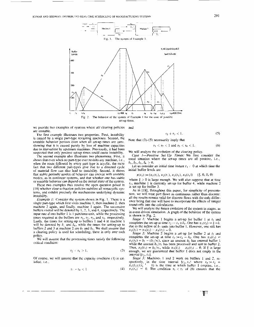
Fig. 1. The system of Example 1.

11 12 t314 1- 16 17 it i9 il0 i11i,2 11430Time

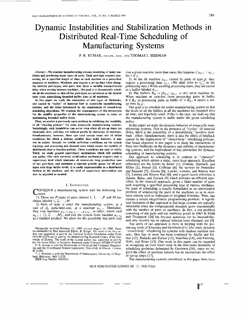
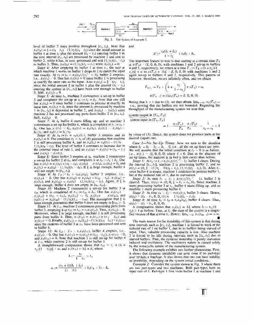
Fig. 2. The behavior of the system of Example 1 for the case of positive set-up times.

we provide two examples of systems where all clearing policies are unstable.

The first example illustrates two properties. First, instability is caused by a single part-type revisiting machines. Second, the unstable behavior persists even when all set-up times are zero, showing that it is caused purely by loss of machine capacities due to starvation by upstream machines. Previously, it had been suspected that only positive set-up times could cause instability.

The second example also illustrates two phenomena. First, it shows that even when no part-type ever revisits any machine, i.e., when the route followed by every part-type is acyclic, the mere fact that two different part-types give rise to a directed cycle of material flow can also lead to instability. Second, it shows that stable periodic modes of behavior can coexist with unstable modes, as in nonlinear systems, and that whether one has stable or unstable behavior can depend on the initial state of the system.

These two examples thus resolve the open question posed in [ 181 whether clear-a-fraction policies stabilize all nonacyclic systems, and exhibit precisely the mechanisms underlying dynamic instability.

Example I : Consider the system shown in Fig. 1. There is a single part-type which first visits machine 1 , then machine 2, then machine 2 again, and finally, machine 1 again. The successive buffers visited will be denoted by 1, 2 , 3, and 4, respectively. The input rate d into buffer 1 is 1 padtime-unit, while the processing times required at the buffers are 71, 7 2 , 7 3 , and 74, respectively. Lastly, the times for setting-up to buffers 1 and 4 at machine 1 will be denoted by 61 and 6 4 , while the times for setting-up to buffers 2 and 3 at machine 2 are 6 2 and 6 3 . We shall assume that a clearing policy is used for scheduling; there is only one such policy.

We will assume that the processing times satisfy the following critical condition:

7 2 + 74 > I . (3)

Of course, we will assume that the capacity condition ( 1 ) is sat- isfied, i.e.,

71 +74 < 1 (4)

and

72 + 7 3 < 1. ( 5 )

( 6 )

We will analyze the evolution of the clearing policy. Case I-Positive Set-Up Times: We first consider the

usual situation where the set-up times are all positive, i.e.,

Let us consider an initial time instant t = 0 at which time the

Note that (3)-( 5) necessarily imply that

71 < 7 2 < 1 and 7 3 < 7 4 < 1.

61, 6 2 , 63 , 64 ? 0.

initial buffer levels are

x(t1) := (Xl( t l ) , X2(tl), X3(tl), X4(tl)) = ( E , 0, 090) where 4 > 0 is large enough. We will also suppose that at time t 1 , machine 1 is currently set-up for buffer 4, while machine 2 is set-up for buffer 3.

As in [18], throughout this paper, for simplicity of presenta- tion, we will treat part flows as continuous rather than discrete; all the results remain valid for discrete flows with the only difference being that one will have to incorporate the effects of integer round-offs into the calculations.

We will analyze the future evolution of the system in stages, as in event-driven simulation. A graph of the behavior of the system is shown in Fig. 2.

Stage I : Machine 1 begins a set-up for buffer 1 at tl and completestheset-upattimet2 := t1+61.One hasxl(t2) = t + 6 1 due to the inflow of 61 units into buffer 1. However, one still has

Stage 2: Machine 2 begins a set-up for buffer 2 at t2 and completes the set-up at time 1 3 :=t2 + 6 2 . One has x l ( t 3 ) = xl( t2) + 62 - (62/rl), since an amount 6 2 has entered buffer 1 while the amount 62/71 has been processed and sent to buffer 2 . Thus, xz(t3) = 62/71, while x3(t3) = xq(t3) = 0. If E is large enough, we are guaranteed that buffer 1 does not empty in the interval [ tz , t 3 ] .

Stage 3: Machines 1 and 2 work on buffers 1 and 2 , respectively, in the time interval [ t 3 , t 4 ] where 14 := t 2 + x l ( t 2 ) / ( r F 1 - 1) is the time at which buffer 1 empties, i.e., x1(t4) : 0. The condition 71 < 72 of (6) ensures that the

XZ(t2) = X3(t2) = Xq(t2) = 0.

~

292 IEEE TRANSACTIONS ON AUTOMATIC CONTROL. VOL. 35, NO. 3 , MARCH 1990

Machine 1 3 L

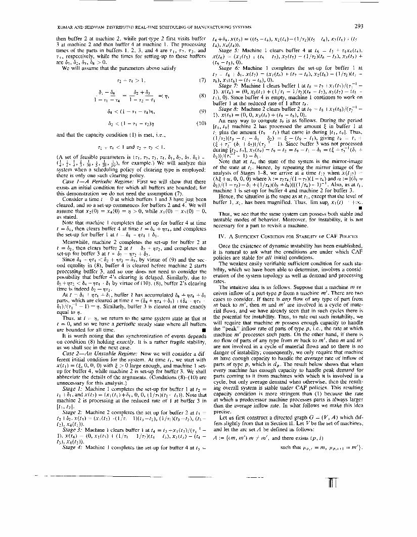
Fig. 3 . I4

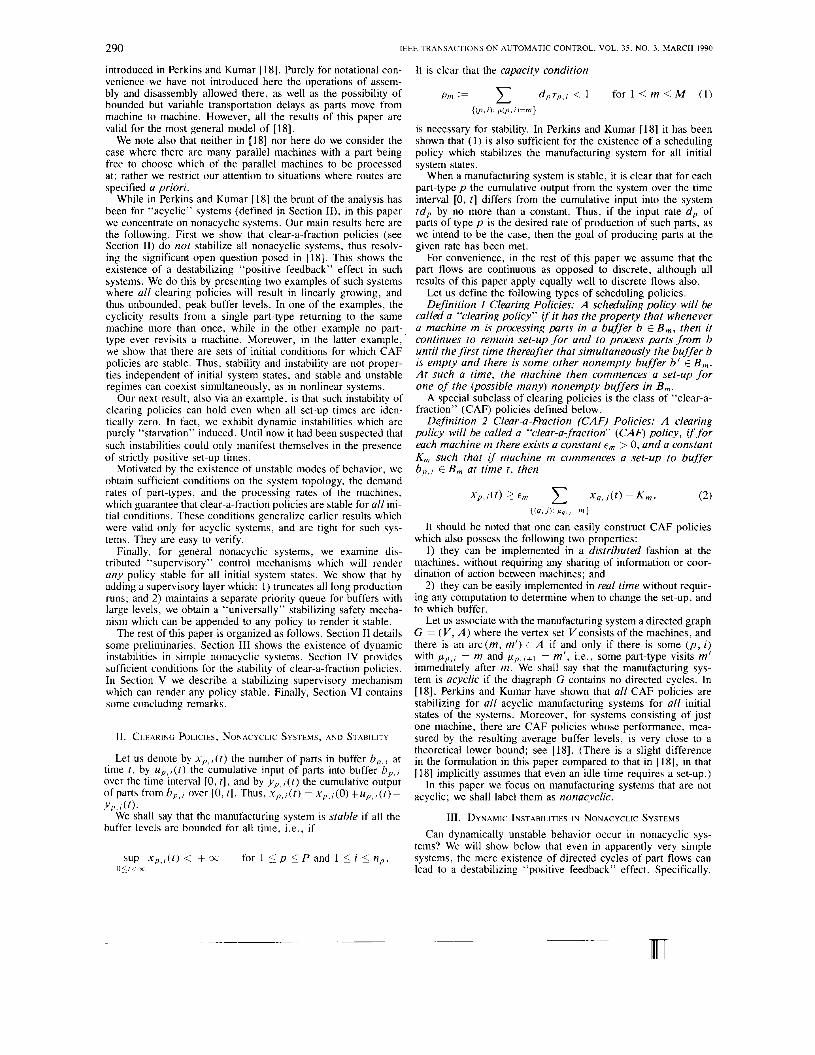
The system of Example 2

level of buffer 2 stays positive throughout [ t 3 , t 4 ] . Note that x ~ ( t 4 ) = [ + ( t 4 - t 1 ) - ( 1 / 7 2 ) ( t 4 - t 3 ) since the initial amount in buffer 1 at time tl plus the amount ( t 4 - t l ) entering buffer 1 in the time interval [ t I, t4J are processed by machine 1 and sent to buffer 2 , while it has, in turn, processed and sent (1 /72)(t4 - fj) to buffer 3. Thus, x 3 ( t d ) = ( 1 / 7 2 ) ( t 4 - t ,) while x q ( f 4 ) = 0.

Stage 4: After emptying its buffer 1 at time 14, the rate at which machine 1 works on buffer 1 dro s to 1 to match the input rate exactly. At t 5 : = t 4 +x2(t4)/(72 - I ) , buffer 2 empties, i.e., ~ 2 ( t 5 ) = 0. One has xl(fS) = 0 since buffer 1 is processing at exactly the same rate as the input. Also x j ( t 5 ) = 4 + ( f 5 - t l ) , since the initial amount E in buffer 1 plus the amount ( t s - t l )

entering the system in [ t l , t5] have been sent through to buffer 3. Still, X 4 ( t 5 ) = 0.

Stage 5: At time t 5 , machine 2 commences a set-up to buffer 3 and completes the set-up at t 6 := t 5 + &. Note that one still has xl(t6) = 0 since buffer 1 continues to process at exactly its input rate, X z ( t 6 ) = 63 since the amount 6 3 processed by machine 1 in [ t 5 , t 6 ] is deposited in buffer 2, and x3( t6) = x3(ts) since machine 2 has not processed any parts from buffer 2 in [ t s , t61. Still, x q ( t 6 ) = 0.

Stage 7: At 16 buffer 4 starts filling up, and so machine 1 commences a set-up for buffer 4, which is completed at r7 := t h + 6 4 . One has X l ( t 7 ) = 64, X 2 ( t 7 ) = x ~ ( t 6 ) , x 3 ( f 7 ) = x 3 ( f 6 ) -

6 4 / 7 3 , and x 4 ( t 7 ) = 64 /73 . Stage 6: At t g : = t 7 + r3x3(r7), buffer 3 empties and so

x3(fx) = 0. The condition 5 < 74 of (6) guarantees that machine 1 is still processing buffer 4, and so X q ( t 8 ) = xq(f7) - ( 1 /74 -

l / q ) ( t g - t 7 ) . The level of buffer 1 continues to increase due to the external input of rate 1 , and so x l ( l8 ) = xl(t7) + ( f 8 - t 7 ) and X 2 ( f S ) = x2(t7).

Stage 8: Since buffer 3 empties at t g , machine 2 commences a set-up for buffer 2 at f g , and completes it at t 9 := tg + 62. One hasxl(t9) =xl( td+(h - tx) ,x2( t9) = x 2 ( t d , x 3 ( 1 ~ ) = O , and x4(t9) = x4(t8) - ( l / r 4 ) ( t 9 - t g ) . If is large enough, buffer 4 will not empty in [ t s , ty ] .

Stage 9: At t l o : = t 9 + ~ x 2 ( t g ) , buffer 2 empties, i.e.,

X 2 ( f 9 ) , and xq(f10) = xq(t9) - ( 1 / 7 4 ) ( t 1 0 - 1 9 ) . Again, if E is large enough, buffer 4 does not empty in [ ty , t l o ] .

Stage IO: Machine 2 commences a set-up for buffer 3 at t l o which is completed at f l l : = t l o + 6 3 . One has x l ( t l l ) = x l ( f l 0 ) + ( ~ I I - IO), X Z ( ~ I I ) = 0, x3(t11) = x3(tlO), and x4(tll) = ~ ~ ( 1 1 0 ) - ( 1 / 7 4 ) ( t l l - t l o ) . The assumption that [ is large enough guarantees that buffer 4 does not empty in [ t l o , t I I ] .

Stage 11: At tl I, machine 2 commences processing parts from buffer 3, emptying it at t12 := t l ~ + 7 3 ~ 3 ( f 1 1 ) . Thus, x3(tl2) 7 0. Moreover, when 4 is large enough, machine 1 is still processing parts from buffer 4. Thus, xl(t12) = x I ( f I I ) + ( t 1 2 - ~ I I ) and x ~ ( t 1 2 ) = 0. Finally, X4(f12) = ~ 4 ( t 1 1 ) - ( 1 / 7 4 ) ( t 1 2 - t 1 1 ) + X 3 ( t l l ) since the contents of buffer 3 at t l 1 have been processed and sent to buffer 4 .

Stage 12: At f I 3 : = t 1 2 + 74x4( t12) , buffer 4 empties, i.e., x 4 ( t 13) = 0. One has x1 ( t i 3 ) = X I ( 1 1 2 ) + ( t l 3 - t12), ~ ~ ( 1 1 3 ) = 0, and x3(t13) = 0. Note that machine 1 is still set-up for buffer 4 at t 1 3 , while machine 2 is still set-up for buffer 3.

A straightforward computation shows that r I 3 = t l + ( h + 72 / (1 - T Z ) ) ~ +CY, and x 1 ( t 1 3 ) = XC; + p , where

P

x 2 ( f 1 0 ) = 0. One has xl(t l0) = x l ( t 9 ) + (tlo - t ~ ) , x3(tlO) =

74 > 1 , := ___ 1 - 72

(74 + 1)(61 + 6 2 )

( 1 - 7 2 ) + 63(74 + 1) + 64 CY :=

and

74(81 + 62) + 7463 + 64. p := 1 - 7 2

The important feature to note is that starting at a certain time To at x ( T 0 ) = ( E , 0, 0, 0), with machines 1 and 2 set-up to buffers 4 and 3, respectively, we return at a time T I := T O +(A +TZ /( 1 - ??) )E + a to TI) = (A[ + p, 0, 0, 0) with machines 1 and 2 again set-up to buffers 4 and 3, respectively. This pattern of behavior, therefore, recurs infinitely often, and we obtain

x(T,+I) 1 ( h l ( T n ) +b , 0, 0, 0).

Noting that X > 1 due to (3), we thus obtain limn-x x l ( T , ) = +x, proving that the buffers are not bounded. Regarding the throughput of the manufacturing system we note that,

system output in [To, T,] system input in [To, T,]

Xl(T , ) -x1(To) ; = I - < 1

by virtue of (3). Hence, the system does not produce parts at the desired (input) rate.

Case 2-No Set-Up Times: Now we turn to the situation where h1 = 62 = 63 = 64 = 0, i.e., all the set-up times are zero. We will assume that the initial condition at t I = 0 is as before, i.e., x ( t l ) = ( E , 0, 0, 0) where t: > 0. Due to the absence of set-up times, the analysis is in fact a little easier than before.

Stagel: Attz : = t l + x l ( t l ) / ( ~ ; l - l ) , buffer 1 clears. During the interval [ t i , 121 , machine 2 is processing buffer 2, and so

since buffer 4 is empty, machine 1 continues to process buffer 1 , but at the reduced rate of I , due to starvation.

Stage 2: At time t 3 = 1 2 + x 2 ( f 2 ) / ( 7 F 1 - l ) , buffer 2 is cleared. Thus, x( t3) = (0, 0, E + r3 - t l , 0). Since machine 2 starts processing buffer 3 at t 3 , buffer 4 starts filling up, and so machine 1 starts processing buffer 4.

Stage 3: At time t 4 = t 3 + 7 3 ~ 3 ( t 3 ) , buffer 3 clears. Hence, w4) = (t4 - f 3 , 0 , 0,

Stage 4: At time t5 = t4 + r4x4(t4), buffer 4 clears. Thus, X ( f 5 ) = ( 1 5 - t 3 , 0, 0, 0).

A computation shows that x l ( t 5 ) = where h :=r4 / (1 - 72) > 1 as before. Thus, at t 5 , the state of the system is a magnified version of that at time t l . Hence, x l ( k n + l ) = +x.

The main reason for the instability of this system is that during time intervals such as [ t2 , t3], machine 1 is forced to work at the reduced rate of 1 on buffer 1 , due to its buffers being starved of input. Thus, valuable processing capacity is lost. Also machine 2 is forced to be idle during intervals such as [ t 4 , f 5 ] due to starved buffers. Thus, the dynamic instability is purely starvation induced and oscillatory. The oscillatory nature is caused solely by the nonacyclic nature of the manufacturing system.

The following example exhibits two further phenomena. First, it shows that dynamic instability can arise even if no part-type ever revisits a machine. It also shows that one can have stability or instability, depending on the system initial conditions.

Example 2: Consider the system shown in Fig. 3 where there are two part-types and two machines. Both part-types have an input rate of 1 . Part-type 1 first visits buffer 1 at machine 1 and

Tn -TO 7 2 + 74

x ( f 2 ) = (0, E : ( 1 / 7 ~ - l ) ( t ~ - t l ) , (1!72)( f2 - t l ) , 0). After t 2 ,

- 1/74)(14 - t3)) .

KUMAR AND SEIDMAN: DISTRIBUTED REAL-TIME SCHEDULING OF MANUFACTURING SYSTEMS

then buffer 2 at machine 2, while part-type 2 first visits buffer 3 at machine 2 and then buffer 4 at machine 1. The processing times of the parts in buffers 1, 2, 3, and 4 are T ~ , 7 2 , 7 3 , and 74, respectively, while the times for setting-up to these buffers are 61, 63, 64 > 0.

We will assume that the parameters above satisfy

72 + 7 4 > 1 , (7)

and that the capacity condition (1) is met, i.e.,

71 + 74 < 1 and 72 + 73 < 1.

(A set of feasible parameters is (71, 7 2 , 73, 74, 61 , 6 2 , 6 3 , 6 4 ) =

system when a scheduling policy of clearing type is employed; there is only one such clearing policy.

Case I-A Periodic Regime: First we will show that there exists an initial condition for which all buffers are bounded; for this demonstration we do not need the assumption (7).

Consider a time t = 0 at which buffers 1 and 3 have just been cleared, and so a set-up commences for buffers 2 and 4. We will assume that x2(0) = xq(0) = 17 > 0, while x l (0) = x3(0) = 0, as stated.

Note that machine 1 completes the set-up for buffer 4 at time 1 = 6 4 , then clears buffer 4 at time t = B4 + 1774, and completes the set-up for buffer 1 at t = 64 + 1774 + 61.

Meanwhile, machine 2 completes the set-up for buffer 2 at t = 6 2 , then clears buffer 2 at t = 6 2 + 1772, and completes the set-up for buffer 3 at t = 62 + 17r2 + b3.

Since 64 + 1774 < 62 + 17/72 + 63, by virtue of (9) and the second equality in (8), buffer 4 is cleared before machine 2 starts processing buffer 3, and so one does not need to consider the possibility that buffer 4’s clearing is delayed. Similarly, due to 62 +1772 < 64 +1774 +61 by virtue of ( lo ) , (8), buffer 2’s clearing time is indeed 62 + 1772.

At I = 64 + 17/74 + 61, buffer 1 has accumulated 64 + 1774 + 61 parts, which are cleared at time t = (h4 + 0 7 ~ + 6,) + (ti4 + 1 7 ~ ~ + 61)/(7F1 - 1) = 17. Similarly, buffer 3 is cleared at time exactly equal to 7.

Thus, at t = 17, we return to the same system state as that at t = 0, and so we have a periodic steady state where all buffers are bounded for all time.

It is worth noting that this synchronization of events depends on condition (8) holding exactly. It is a rather fragile stability, as we shall see in the next case.

Case 2-An Unstable Regime: Now we will consider a different initial condition for the system. At time I , , we start with x ( t l ) = ( E , 0, 0, 0) with 4 > 0 large enough, and machine 1 set- up for buffer 4, while machine 2 is set-up for buffer 3. We shall abbreviate the details of the arguments. (Conditions (8)-( 10) are unnecessary for this analysis.)

Stage 1: Machine 1 completes the set-up for buffer 1 at r 2 = I , +61,andx( t2) = ( x l ( t l ) + 6 , , 0, 0, ( l / 7 3 ) ( f 2 - t l ) ) . Notethat machine 2 is processing at the reduced rate of 1 at buffer 3 in

Stage 2: Machine 2 completes the set-up for buffer 2 at t3 =

Stage 3: Machine 1 clears buffer 1 at t4 = t 3 +xl(t3)/(7;’ -

Stage 4: Machine 1 completes the set-up for buffer 4 at t 5 =

(1 4 , 1 2 , 4, I z 3 , 1 30, L s , I 2 0 , L ) 2o , f or example.) We will analyze this

[tl, t21.

1 2 +62. x(t3) = ( x l ( t 2 ) - ( 1 / ~ ~ - 1)(t3 - t 2 ) , (1/7, ) ( t3 - t ? ) , ( r 3 - f 2 ) , X4([2)).

1). x(t4) = (0 , xz( t3) + (1/71 - 1 / ~ ) ( t ~ - r 3 ) , x3(r3) + ( r 4 - t 3 1 , X4([3)).

~

293

t4 +h4. x( i3) = ( ( t s -t4L ~ 2 ( f ~ ) - ( 1 / ~ ~ ) ( f ~ -t4), X3([4)+(fS - t4), x4(t4)).

Stage 5: Machine 1 clears buffer 4 at t 6 = t5 + 7414(t4). X(t6) = (xl(tS) + (16 - t S > > x2(15) - (1/7Z)(f6 - t 5 > 9 X 3 ( t 5 ) + ( I 6 - t 5 ) 9 0).

27 = t 6 + 61. w 7 ) = (xI(16) + (17 - f6)9 XZ(t6) - (1/72)(t7 - 7619 X3(t6) + (17 - t6)9 0).

Stage 6: Machine 1 completes the set-up for buffer 1 at

Stage 7: Machine 1 clears buffer 1 at r 8 = t 7 +xl(t7)/(7;I -

t7), 0). Since buffer 4 is empty, machine 1 continues to work on buffer 1 at the reduced rate of 1 after t g .

Stage 8: Machine 2 clears buffer 2 at ty = f8 +x2(ts)/(7TT?I -

An easy way to compute ty IS as follows. During the period [ t , , ty] machine 2 has processed the amount 5 in buffer 1 at t l plus the amount (ty - t l ) that came in during [ f l , t g ] . Thus, ( 1 / 7 2 ) ( t q - t l - 6l - 6*) = E + (ty - t , ) , giving tg = tI + ( E + 7; (61 + 62))/(7F1 - I). Since buffer 3 was not processed during [ t t , r91, x 3 ( t ~ ) = 19 - 12 = 19 - f l - 61 = (t + 72’(61 +

Note that at ty, the state of the system is the mirror-image of the state at t l . Hence, by repeating the mirror image of the analysis of Stages 1-8, we arrive at a time ti7 when x ( t I 7 ) = ( X ~ + a ! , O , O , O ) w h e r e X : = ~ 2 7 ~ / ( 1 - ~ 2 ) ( l - ~ ~ ) a n d c u : = [ ( 6 1 + 62)/(1 - ~ 2 ) - 6 1 +(1/74)(63 +64)]((1/~4)- I)-’. Also, as at II, machine 1 is set-up for buffer 4 and machine 2 for buffer 3.

Hence, the situation is the same as at t l , except that the level of buffer 1, X I , has been magnified. Thus, lim supt X I ( t ) = +m.

H Thus, we see that the same system can possess both stable and

unstable modes of behavior. Moreover, for instability, it is not necessary for a part to revisit a machine.

1). x ( t d = (0, x2( t7) + (1/71 - 1 / 7 ~ ) ( t ~ - f 7 ) , x3(t7) + Us -

1). x(tY) = (0, 0, X3(t8) + (tY t 8 ) 9 0).

6 2 ) ) / ( 7 1 - 1 ) - 61.

IV. A SUFFICIENT CONDITION FOR STABILITY OF CAF POLICIES

Once the existence of dynamic instability has been established, it is natural to ask what the conditions are under which CAF policies are stable for all initial conditions.

The weakest easily verifiable sufficient condition for such stability, which we have been able to determine, involves a consid- eration of the system topology as well as demand and processing rates.

The intuitive idea is as follows. Suppose that a machine m re- ceives inflow of a part-type p from a machine m’. There are two cases to consider. If there is any flow of any type of part from m back to m‘, then m and m‘ are involved in a cycle of material flows, and we have already seen that in such cycles there is the potential for instability. Thus, to rule out such instability, we will require that machine m possess enough capacity to handle the “peak” inflow rate of parts of type p , i.e., the rate at which machine m’ processes such parts. On the other hand, if there is no flow of parts of any type from m back to m‘, then m and m’ are not involved in a cycle of material flows and so there is no danger of instability; consequently, we only require that machine m have enough capacity to handle the average rate of inflow of parts of type p , which is d,. The result below shows that when every machine has enough capacity to handle peak demand for parts coming to it from machines with which it is involved in a cycle, but only average demand when otherwise, then the resulting overall system is stable under CAF policies. This resulting capacity condition is more stringent than (1) because the rate at which a predecessor machine processes parts is always larger than the average inflow rate. In what follows we make this idea precise.

Let us first construct a directed graph G = ( V , A ) which differs slightly from that in Section 11. Let V be the set of machines, and let the arc set A be defined as follows:

A := { ( m , m’)lm # m’, and there exists ( p , i) such that p p , l = m , p p , r + ~ = m ’ } .

294

The only difference between the graph defined here and that in Section I1 is that here we eliminate all “self-loops’’ consisting of arcs of the form (m , m) from A . (Thus, the graph G defined here may have no directed cycles, and yet the manufacturing system can still be nonacyclic as defined in Section 11.)

We shall say that m’ is reachable from m if there is a directed path from m to m’; we shall write this as “m + m’.” If m + m’ and m’ + m, we shall say that m and m’ are diconnected, and write “m c-) m‘”. By convention, we shall always say that m c--t m. Note that “ - ” is an equivalence relation; hence, it partitions V into disjoint sets G 1 , . . . , G, with the properties that: 1 ) m tf m‘ if and only m, m’ E G, for some i; 2) GI nG, = C#J for i # j ; and 3) U,G, = V .

On {G 1 , . . . , G, } we have the following induced partial ordering. We will say that G, -+ G, if and only if there exist m E G I , m’ E G, with m + m’.

Our sufficient condition for stability of CAF policies is given by the following theorem.

Theorem I : For each buffer bP, , define

Ap, l :=0

: = j

if pP, , = p p , l for all j 5 i ,

if p p , , # p p , , but F p , k = p p , l for j + 1 5 k 5 i ( 1 1 )

and then define the ‘prior machine’’ T ~ , ~ visited by Wrt-type p as follows:

rp,; := C#J if AP,; = 0,

(12) For each buffer bp,; we next define the “modified input rate” db,; as follows:

d;,, :=d,

._ .- pp, A,,, otherwise.

if either rp,; = 4 or T ~ , ;

is not diconnected with p p , i ,

If the more stringent capacity condition,

p; := d;,;Tp,; < 1 for all m (14)

holds, then all CAF policies are stable for all system initial conditions.

Proof: Let us consider the equivalence classes of machines G I , . . . , G, induced by the relation “ c-) ”. As noted earlier, on { G I , . . . , G r } there is a natural partial ordering “-+”, and let {GI, . . . ,GI }, say, be the set of minimal elements with respect to this partial ordering. (We say that G; is “minimal” if there is no G, such that Gj 4 G;.)

First we will show that all the buffer levels at the machines in any of these minimal elements are bounded. For the sake of definiteness, consider a machine m E G I .

{Cos;): p,, ,=m>

For each buffer bp,; with pp, ; = m we define

qp, ; := max { j : pp,k = m for i 5 k 5 i + j - I }

and note that ( q p , ; - 1) is the number of times that part-type p subsequently “loops back” to m before visiting another machine or exiting from the system.

We shall consider the following “Lyapunov function”:

V m ( t ) := X p , i ( f ) [ T p , i +7p,i+l + “ ’ f T p , i + q a . , - l l .

{Co.,): a p , , = m }

(15)

Let {T,} be the sequence of times at which machine m commences a set-up, and let ( p i , i i) denote the buffer selected for

IEEE TRANSACTIONS ON AUTOMATIC CONTROL. VOL. 35. NO. 3. MARCH 1990

the set-up of m commenced at time Tn . Note that by the property (2) of CAF policies

X p ; , i ; V n ) L em xp,i(Tn) - ~ m *

{(P,i). p , , , = m )

For any ( p , i ) with pp, ; = m E G I , if rp,; = 6, then pp, ; is the first machine visited by part-type p . If ap,; f 4, then there is some prior machine T ~ , ; E { 1, 2, . . , M } , different from m. Note that since part-type p moves from aP,; to p p , ; , we have T ~ , ; -+ p p , ; . If pp, ; f c P , , , then this would violate the minimality of G I . Hence, pp, ; - T ~ , ; . Thus, we see that the only two possibilities are rP, ; = 4, or rp,; c-) p p , ; . Hence, by the definition of d; ; in (13), either d; I = d p in which case part-type p enters the’system at machine h, or db,i = ( 1 / r p , k , , , ) . Since ~ / T ~ , X ~ , , is the maximum rate at which parts can move out to buffer bp,A,,, to buffer bp,; and into m, it follows that in either case, the maximum rate of entry of parts into m is db,,. Thus,

where work is measured in time-units that machine m would take to process.

Now we consider two cases. If machine m has been active during the entire period [T , +8bp:-I,,;-I ,b,:, ,;, T,+I] , then one has,

Vm(Tn+I) I V(Tn) + c { (a . ; ) : p P . , = m , p p . , - I f m }

. d;.;bp,; + Tp,;+1 + ’ ’ . + 7p , ;+q p . , - ~ l ( T n + ~ - T n )

- (Tn+I ~ T n ~ 8bp;_ bp:. ,;)

since by (16) the first term in the above summation represents an upper bound on the work that has arrived in the interval [T,, T,+l], while the second term in the summation represents the work done in [T, + 8bp;- l , , ; - l ,b,;,,;, T,+I] . On the other hand, machine m could have been forced to process at less than the maximum rate due to starvation, which happens when V , ( S ) = 0 for some s E (T, , T ,+I] . But then, since (14) im- plies d; ; < ( 1 / r P , ; ) , the rate at which work enters in the interval [s, f , + ~ ] is less than the rate at which it is completed, and so it follows that V m ( t ) = 0 for s 5 t 5 T,+l, and in particular V,(T,+l) = 0. Hence, in either case, one has the inequality,

r

KUMAR AND SEIDMAN: DISTRIBUTED REAL-TIME SCHEDULING OF MANUFACTURING SYSTEMS 295

where the last equality follows from the definition in (14). Hence, (17) simplifies to

Vrn(Tn+I) 5 max[O, Vm(TnIP(1 - ~ : n ) ( ~ n t I - ~ n ) + 6 1

(18)

where 8 := maXb,b‘tB,, 6b.b’ > 0. As a consequence of (18) one has the following implication:

Moreover, by the “clearing” property

Also, by the CAF property (2)

Finally, by ( 15)

( 2 2 )

Ttn := max

This proves the ultimate boundedness of Vm(T,) , and thus also of V , ( t ) since V , ( t ) i V,,(T,) + 6 p k for all t E [T,, T,,-1].

Thus, we have shown that the levels of the buffers of all the machines in the minimal elements G I , . . , G/ are bounded by, say, r.

The proof now proceeds by induction. Since the remaining steps of the induction are all similar, for simplicity of notation we show the second step of the induction process only.

Let us now delete these minimal elements from {G ’ . , G, }, and consider the reduced set { G I + I , . . . , G , } with the same (i.e., a restriction of the) partial order “+” as before. Let G / + I , ‘ . . , G / + q , say, be the new minimal elements of {G/+1 l . . . ,Gr,} with respect to the partial order “+”. Consider an arbitrary minimal element, say G / + I , and consider an arbitrary machine m in it, i.e., m t G/+1.

Let us fix attention on the buffer b,,i E B, . If ap,i = 4, then part-type p enters the system at m , and so the rate of entry of such parts is d’ . = d , by (13). If not, then there is a previous machine a,,; {’(l,. . . , M } visited by the part-type p . Note that rp,[ U L-,+zCn since that would violate the minimality of G I + ~ . Hence, either P ~ , , E G/+I or T ~ , ; t U‘, . If r,,, E G / + l , then since db,, := (1 /~ , , ; ) by (13). it follows that the maximum

n rate at which parts move E o m b,,, i,,, to m is d;,,. Lastly, if ap,, E U/,zlG,, then a,,k E U n r l G , for all 1 < k < i - 1, since G I, . . . ,G, were originally minimal, and so part-type p enters the system at a rate d, at one of the machines in U i=lG,, . However, since all the buffers of such machines are bounded by

Inflow of parts in [T,, T,,+ll L dh,,[T,+I - T , ] + r (23)

since d;,, := d, in this case. Note therefore, that in all cases, one has an inequality such as

(23) (where r can even be set to 0 in the first two cases), and so

r,

Inflow of work to m in [T,, T n + t ]

i c {db,;t7p,i +...+7 p , i + ~ , , , - - ~ l

{ w , J ) : p p . , - m , p , . , . ~ # m }

‘ (Tn+t -Tn)+U7,,, + . . . + 7 p , i + 7 p . , - ~ ) }

= Pk(T,+l - T,) + I; -

where 1’ := E{(,,,) P P , , - - m , p , , , - , #,} r [ 7 P , r + ’ ’ . + 7 p , i t g ,,,, -11. This is a simple generalization of the bound in (16).

Now let us examine the work done by machine m in the time interval [T,, + h o p ; - ,,,; , ,b,:, ,:, Tntl], in which period machine tn is active. If it did nof process at the maximum rate of ( 1 /T,,;,,;) throughout this time interval, then there is a time instants E ( T , , T,+I] at which V ( s ) = 0, since machine m must have been starved at some such time instant. If s = T , , I, then V,(T,,-l) = 0. If not, let s be the last such time instant. In [s, T n L 1 ] , machine m works at the maximum rate, and so the work completed is ( T , + I - s). However, then the work entering in [s, T,+I] can be at most P:,~(T,+~ - s) + r.

Thus, by covering all cases, we obtain the relation Vm ( T n + l )

< max 0, V n , ( T , ) - (1 - PA,) (T~+I - T n ) { -

f 6b,2:, ,;, b,,:, ,: + I’,

5 max {F, V?,?(T,) - ( I - P L l ) ( T n - l - T,) + %,,; ,; + rI which is a simple generalization of the recurrence bound (17). Thus, by repeating the earlier arguments, we obtain the ultimate boundedness o f Vm(T,). The boundedgess of Vm ( t ) follows by noting that V,(t) < V m ( T , ) + 6 p ; + r for all t t [T,, T n T I ] .

Continuing by induction, one can next remove {G/+l , . . . , G/ + q } , and by a repeated application of this technique, the

proof is completed.

V. A UNIVERSALLY STABILIZING SUPERVISORY MECHANISM The sufficient condition (14) for CAF policies to be stable

for all system initial conditions is a more stringent requirement than the capacity condition ( 1) since p:, 2 ,om. Hence, rather than restrictively requiring (4) to hold, we are interested in obtaining policies which are stable whenever (1) holds. However, as shown in Section 111, dynamic instability is a very real possibility. Is there a simple “stabilization” mechanism by which a supervisor can modify any scheduling policy so that it becomes stable when only (1) holds?

We will now show there does exist such a “universal” safety mechanism, which can moreover be trivially implemented by a supervisor, in a distributed fashion, at the various machines. Es- sentially this mechanism consists simply of

1) truncating all long production runs; and 2) maintaining a separate first-come first-serve (FCFS) prior-

ity queue QnI for large buffers, at each machine m .

For each machine m , let ym be a large number satisfying 4) Suppose [ t , t’] is any interval such that

Since pm < 1 by capacity condition ( I ) , such a choice is clearly feasible. Second, we shall arbitrarily choose for each buffer bP, , a nonnegative number z P , , . The precise operation of the supervisor is given by the following five rules to be implemented in a distributed fashion at each machine m.

The Truncation Rule: No processing run of buffer bp, ! at machine m is ever allowed to continue beyond YmdpTPp,, time units.

The Rule for Entering Qm: A buffer bP, , enters the tail of the priority queue Qm if: 1) b P , , is not being processed or set-up; and 2) its buffer level xp,, exceeds z P , , .

The Buffer Selection Rule: If Qm f C#I when a processing run terminates, then the buffer at the head of the priority queue Qm (i.e., according to a FCFS discipline) is chosen next for processing.

The Rule for Leaving Qm: A buffer leaves the priority queue Qm when it is taken up for processing, i.e., a set-up is commenced.

The Rule for the Processing Time for a Buffer from Qm: If a buffer b P , , from Qm is taken up for processing, then it is processed for exactly ymdp rp , , time units, unless it clears before this amount of time has elapsed.

It should be noted that the above rules do not restrict in any way which buffer is chosen for processing if Qm is empty. Thus, except for the truncation rule, the supervisory mechanism intervenes only when buffer levels become large, and is otherwise unobtrusive.

A second point to note is that after completing a processing run, a buffer bP, , may immediately enter Q m ; this happens if its buffer level at the end of the processing run is larger than zp, ,,.

It is worth mentioning that there is considerable flexibility in choosing the frequency of supervisory intervention. For example, if zp , , := 0, then the supervisor simply enforces a first-come-first- serve (FCFS) discipline among the nonempty buffers, truncating their processing runs after -ymdpTp,, time units. Thus, the supervisor always intervenes. On the other hand, if a policy is already stable, and if both z p , , and Y m are chosen large enough, then the supervisor never intervenes. Hence, by choosing zp, I and ym , the degree of supervisory intervention can be adjusted.

In what follows we prove that this supervisory mechanism guarantees stability.

The following preliminary lemma exhibits four key consequences of the supervisory mechanism.

Lemma I : Suppose buffer bP, , enters Qm (where m = p P , , ) at a time instant t , , and has its subsequent processing run completed at a time tcomplete.

I ) Then

where

x p , , ( u ) 2 g p , l for all U E [ t , t’]

296 IEEE TRANSACTIONS ON AUTOMATIC CONTROL, VOL 35, NO 3. MARCH 1990

-

Note that {m > 0 by (24). 2) Let Pp, , ( t ) := C : , l ~ p , l ~ p , J ( t ) be the backlog of work

for machine m in the prior buffers visited by part-type p .

3) Suppose t IS such that xp , , (u ) 2 max (ymdp, z,,,) for all a E [t,,, t’]. Then

Thenxp,,(tln) $ Y m d p * Pp,r(tcomplete) I Pp,r(tin)-lmdp7pTp.,.

lm ) / l m h p Tp. i 1. Proof: 1 ) When bo., enters Qm, at worst all other buffers

b E B , can be ahead of bp,i i n Q , . By the truncation rule, allowing for set-up times, buffer bp,; is guaranteed to have its processing run terminated by

which proves 1). 2) If xp,;(ti,) 2 ymdp at a time tin that bp,; enters Q m , then

since its buffer cannot be cleared in less than -ymdp7p,l time units of processing, it follows from the rule for the processing time for a buffer from Qm that the subsequent processing time lasts exactly Y ~ ~ ~ T ~ , ; time units. In the time interval [tinr fcomplete], a quantity dp(tcomplete - ti,) of parts of type p have entered the system at machine p ( p , 1). Thus,

3) The proof is by contradiction. Suppose not, i.e., (t’ - t ) > ( 1 + (Pp,i(tin)/lmdpTp,i))(Ym,- lm)., Let tcomplete > tin be the next time its processing run is terminated. By 1 ) it follows that tL:,&iete - tin 5 -ym - lm, and so t f ~ ~ p l e t e 5 t ‘ . Hence, xp,,(tfbmPlete) 2 lp,; again, and so b p , ; again enters Qnl at tr,” := tLbmplete, and correspondingly let ff2umpiefe be the next time at which it again completes a processing run. Again, by l), ( f c o m p l e t e - tin) I 2 ( ~ m - lm). If now, 2 i (1 + (Pp,i(tin)/ 3;ndp7p,;)), then bp,i again enters Qm at tli’ := tL:mplete, and so on. If n := 11 +(~,,~(tln)/S;rdp~,,In)lS;rtdp7p,i)], then there are n such inter-

( 1 ) (2) I ? ) ( n ) ( n ) vals [tin, f c o m p l e t e 1 , [ti,, , tcomplete1, . . . , [t,, , fcomplete 1 with =

tcomplete for 2 5 k 5 n , at the commencement of each of which,

x P , ; ( t l , , 12 lp,, . Hence, by 21,

( 1 )

(2)

( k - I )

( k )

< O

which is a contradiction, since the backlog Pp, , ( t ) is always nonnegative.

4) At time t since x p , i ( t ) Lz,,;, if bp,; is not in Q m , then it is either being processed or set-up, by the rule for entering Qm . In any event, let s denote the time of the end of the resulting production run. If bp, ; is being processed or set-up at t , then s - i maXb,b’EB, 6bb’ + -ymdp7,,;, where the first term on the right-hand side allows for a set-up time, and the last term represents the maximum length of a production run, due to the

KUMAR AND SEIDMAN: DISTRIBUTED REAL-TIME SCHEDULING OF MANUFACTURING SYSTEMS 297

truncation rule. In case b p , , E Qm at t , then s ~ t 5 ym - {,n by 1). Since Y m - {m > maxb,wa, 6bb’ +~mdp7p , ; by (26), it follows that in all cases

s - t < Y m - {m. (27)

Moreover, by the truncation rule, the number of parts processed in a run is less than or equal to Y m d p . Hence, x p , ;(s) 2 ~ ~ , ~ ( t ) - ymdp 2 m a x ( y m d p , z P , ; ) ; and SO b p , ; enters Qm at time s. By 3) it follows that

and from (27) we thus obtain

Now note that the maximum rate at which P P , ; can grow is dp7p , ; , and so by (27), we have

Substituting in (28) yields the result. Our main theorem concerning the stabilizing property of this

supervisory mechanism is the following. Theorem 2: If the above supervisory mechanism is applied

t o all the machines, then all buffer levels are bounded over all time for all initial system states.

Pro08 Consider any part-type p . We will prove by induction on i that the buffer levels x p , ; ( t ) are bounded for O I t < + 3 O .

visited by part-type p . Note that, as a consequence, P p , ~ ( t ) = T ~ , 1xp, I ( t ) .

Consider the first machine m = p p ,

Let

and inductively define for k 2 1

with the convention that inf 6 := 30. Note that if t ( k ) < +m, then ik < +CO by Lemma 1.4). Moreover, if any t ( k ) = +x, then x p , I ( t ) is bounded (since it is Lipschitz and has no “finite escape time”). So let us suppose t (@ < +m for all k . Note lso that again by the Lipschitz property, if we can prove that It“ - t ( k ) } is a bounded sequence, then x p , 1 ( t ) is bounded.

Let us consider k 2 2, and note that P p , I ( t ( k ) ) = 7p, l x p , I(t(k’) = 7p, l g p , I , and so by Lemma 1.4),

5 ap , I + cp , l g p , 1 7 ~ , I

Since x p , I ( t ) is Lipschitz, it follows that it is bounded.

for all t 2 0, I I j 5 i - 1 .

for all k 2 2. p’ - t‘k’

Now suppose for induction that

x p , ; ( t ) I Ti

Consider b p , ; . Define, as earlier

and inductively define for k 2 1

f ( k + I ) ._ .- inf { t > i ‘ k ’ l x p , l ( t ) = g p , l >.

Again, if t ( k ) = + c c for any k , then x p , r ( f ) is bounded. So let us suppose that t ( k ) < +x for all k . Now note for k 2 2

;-I

i - I

j = l

i-I

Hence, by Lemma 1.4),

Since x p , ; ( t ) is Lipschitz, it follows that it is bounded. The mechanism described above can therefore be used as a

supervisory “safety net” which can be used with any policy to prevent it from dynamic instability. Moreover, it does not require a “centralized” supervisor; a distributed implementation is feasible since each machine can act as its own supervisor.

VI. CONCLUDING REMARKS The present paper provides an analysis of the dynamics of

nonacyclic manufacturing systems. We now have an understanding of the interaction of the feedback effect caused by flows along directed cycles, with the feedback introduced by employing closed-loop scheduling policies.

An important open issue is the obtaining of tight bounds on buffer levels for systems with many machines. For the single- machine case, such bounds are available in [18], and policies, whose performance measured in terms of average weighted buffer levels is very close to a theoretical lower bound, are also available. However, for general systems with many machines, a good understanding is not available, even for the simpler class of acyclic systems. Given the importance of good performance, this issue needs to be properly addressed.

It is also useful to both model and analyze the problem of dynamically scheduling the transportation subsystem. While the machine scheduling algorithms of this paper can be used with any “stable” transportation scheduling policy which guarantees bounded transportation delays, the precise analysis of performance is not available.

Finally, the treatment of random uncertainties such as yields, machine failures, rework, demand changes, etc., is very much of an open, and important problem.

REFERENCES K. Baker, Introduction to Sequencing and Scheduling. New York: Wiley, 1974. R. W. Conway, W. L. Maxwell, and L. W. Miller, Theory of Scheduling. Reading, MA: Addison-Wesley, 1967. S. French, Sequencing and Scheduling. E. G . Coffman, Computer and Job-Shop Scheduling Theory. New York: Wiley, 1976. S . S. Panwalker and W. Iskander, “A survey of scheduling rules,” Operut. Res.. vol. 25, pp. 45-61, Jan.-Feb. 1977. S . Graves, “A review of production scheduling,” Operat. Res., vol.

E. L. Lawler, J . K. Lenstra, and A . H . G . Rinooy Kan, “Recent de-

New York: Wiley, 1982.

29. pp. 646-675, July-Aug. 1981.

298 IEEE TRANSACTIONS ON AUTOMATIC CONTROL. VOL. 3.5. NO. 3. MARCH 1Y90

181

191

11-21

1181

velopments in deterministic sequencing and scheduling,” Determinis- tic and Stochastic Scheduling. Dordrecht, The Netherlands: Reidel. 1982. J . Lenstra and A . H. G. Rinooy Kan, “Sequencing and scheduling,” Preprint. J . Adams, E. Balas, and D. Zawack, “The shifting bottleneck pro- cedure for job shop scheduling,” Management Sci., vol. 34, pp. 391-401, Mar. 1988. J . F . Muth and G. L. Thompson, Industrial Scheduling. Englewood Cliffs, NJ: Prentice-Hall, 1963. J . Kimemia and S. B. Gershwin, “An algorithm for the computer control of production in flexible manufacturing systems,” IEEE Trans., vol. 15, pp. 353-362, Dec. 1983. R . Akella and P. R. Kumar, “Optimal control of production rate in a failure prone manufacturing system,” IEEE Trans. Automat. Contr.,

T. Bielecki and P. R. Kumar, “Optimality of zero-inventory policies for unreliable manufacturing systems,” Operat. Res., vol. 26, pp. 532-546, July-Aug. 1988. A. Sharifnia, “Production control of a manufacturing system with mul- tiple machine states,” IEEE Trans. Automat. Contr.. vol. 33, pp. 620-626, July 1988. W . Fleming, S. Sethi, and M. Soner, “An optimal stochastic production planning problem with randomly fluctuating demand,” SIAM J . Contr. Optimiz., vol. 25, pp. 1494-1502, Nov. 1987. S. B. Gershwin, “A hierarchical framework for discrete event scheduling in manufacturing systems,” in IlASA Workshop on Discrete Event Systems: Models and Applications, Sopron, Hungary, Aug. 3-7, 1987. - “Stochastic scheduling and set-ups in manufacturing systems,” in Proc. 2nd ORSAITIMS Conf. Flexible Manufacturing Syst.: Operat. Res. Models Appl . , K. E. Stecke, Ed. Amsterdam, The Netherlands: Elsevier, 1986, pp. 43 1-442. J . Perkins and P. R. Kumar, “Stable, distributed, real-time scheduling of flexible manufacturingiassemblyidisassembly systems,” IEEE Trans. Automat. Contr., vol. 34, pp. 139-148, Feb. 1989.

vol. AC-31, pp. 116-126, Feb. 1986.

P. R. Kumar (S’77-M’77-SM’86-F’88) was born in India in 1952. He received the B. Tech. degree from the Indian Institute of Technology, Madras. ln- dia, in 1973. and the M.S. and D.Sc. degrees from Washington University, St. Louis, MO, in 1975 and 1977, respectively.

At present he is with the Department of Electri- cal and Computer Engineering and the Coordinated Science Laboratory, University of Illinois, Urbana- Champaign. His current research interests include control systems, manufacturing systems, and neural

networks. He is coauthor (with P. Varaiya) of Stochastic Systems: Estima- tion, Identification and Adaptive Control.

Dr. Kumar is an Associate Editor at Large of the IEEE TRANSACTIONS ON AUTOMATIC CONTROL, Associate Editor of the SIAM Journal of Con- trol and Optimization; Mathematics of Control, Signals and Systems; Systems and Control Letters; and the Journal on Adaptive Control and Signal Processing.

equations (especially sc

Thomas I. Seidman was born in New York in 1935. He received the Ph.D. degree in mathematics from New York University, New York, NY, in 1952.

He has worked in industry and has taught at various universities in the United States and in Europe. Currently, he is Professor of Mathematics at the University of Maryland, Baltimore County. His active research interests currently center on distributed parameter control theory, switching systems. in- verse problems, and nonlinear partial differential

miconductor modeling and free boundary problems).

Documents

Dynamic instabilities and stabilization methods in distributed real-time scheduling of manufacturing systems