Dynamic modeling of photovoltaic module for real-time maximum power tracking

Dynamic modeling of photovoltaic module for real-time maximum power trackingMohammad Saad Alam and Ali T. Alouani

Citation: Journal of Renewable and Sustainable Energy 2, 043102 (2010); doi: 10.1063/1.3435338 View online: http://dx.doi.org/10.1063/1.3435338 View Table of Contents: http://scitation.aip.org/content/aip/journal/jrse/2/4?ver=pdfcov Published by the AIP Publishing Articles you may be interested in Maximum power point tracking of partial shaded photovoltaic array using an evolutionary algorithm: A particleswarm optimization technique J. Renewable Sustainable Energy 6, 023102 (2014); 10.1063/1.4868025 Effects of surroundings snow coverage and solar tracking on photovoltaic systems operating in Canada J. Renewable Sustainable Energy 5, 053119 (2013); 10.1063/1.4822051 Conventional and global maximum power point tracking techniques in photovoltaic applications: A review J. Renewable Sustainable Energy 5, 032701 (2013); 10.1063/1.4803524 Simple and low cost incremental conductance maximum power point tracking using buck-boost converter J. Renewable Sustainable Energy 5, 023106 (2013); 10.1063/1.4794749 Modeling of Radiative Energy Transfer and Conversion in a TPV Power System AIP Conf. Proc. 738, 162 (2004); 10.1063/1.1841891

This article is copyrighted as indicated in the article. Reuse of AIP content is subject to the terms at: http://scitation.aip.org/termsconditions. Downloaded to IP:

216.136.5.154 On: Mon, 07 Apr 2014 14:29:00

http://scitation.aip.org/content/aip/journal/jrse?ver=pdfcov

http://jobs.physicstoday.org/jobs

http://scitation.aip.org/search?value1=Mohammad+Saad+Alam&option1=author

http://scitation.aip.org/search?value1=Ali+T.+Alouani&option1=author

http://scitation.aip.org/content/aip/journal/jrse?ver=pdfcov

http://dx.doi.org/10.1063/1.3435338

http://scitation.aip.org/content/aip/journal/jrse/2/4?ver=pdfcov

http://scitation.aip.org/content/aip?ver=pdfcov

http://scitation.aip.org/content/aip/journal/jrse/6/2/10.1063/1.4868025?ver=pdfcov





http://scitation.aip.org/content/aip/proceeding/aipcp/10.1063/1.1841891?ver=pdfcov

Dm

I

bfmnf

enaos

mtFru

e

a

b

JOURNAL OF RENEWABLE AND SUSTAINABLE ENERGY 2, 043102 �2010�

1

This article is copyright

ynamic modeling of photovoltaic module for real-timeaximum power tracking

Mohammad Saad Alam1,a� and Ali T. Alouani2,b�

1Hybrid Vehicle Development, Chrysler Group LLC, Michigan 48326, USA2Department of Electrical and Computer Engineering, Tennessee Tech University,Tennessee 38505, USA

�Received 21 January 2010; accepted 30 April 2010; published online 8 July 2010�

Today’s society relies heavily on electric power produced mainly using coal andpetroleum. These sources of energy are nonrenewable. The rise in the cost ofpetroleum and the effects of coal on the environment force the issue of seekingalternative sources of energy that are renewable and environmentally friendly. Onesuch source is solar energy. Solar energy is extracted via photovoltaic �PV� mod-ules. The problem with this alternative form of energy is the poor efficiency of solarcells. This work deals with the development of an improved dynamical model ofPV modules to maximize the amount of power extracted from the Sun. The devel-oped model has been implemented using MATLAB

®/SIMULINK. Field data are usedto compare the efficiency of the newly developed model to the existing modelsreported in the available literature. Results reveal that the proposed model led to animprovement of 21% in the efficiency of the PV module. Such improvement inefficiency will lead to great energy saving when used on a large number of PVmodules. © 2010 American Institute of Physics. �doi:10.1063/1.3435338�

. INTRODUCTION

Modern society relies on energy to the point that lives would be entirely interrupted if energyecame unavailable. Energy is used to power our homes, our factories, our cars, planes, and trainsor transportation; our computers for education, product development, business records; and soany other things that we take for granted. Unfortunately, the current sources of energy in use are

onrenewable and are harmful to the environment. The search for renewable and environmentalriendly sources of energy is becoming a necessity to solve the energy problem.

The design of photovoltaic �PV� energy systems, which came into existence in 1958, is anxtensive area for researchers that lately gained vital commercial attraction.1–19 Although there areumerous advancements in the PV technology, the conventional semiconductor based PV modulesre still unable to exhibit efficiency more than 11%–15%.1–5,8,14 Recently, organic PV cells basedn nanotechnology are claimed to have efficiency as high as 40% in laboratory environment, buttill this technology will take time to commercialize.

Although we have other means of artificial energy, such as oil and coal, solar energy is theost abundant natural energy source. Solar energy is free and limitless. In addition, the consump-

ion of solar energy does not harm humans, animals, or the natural environment of the Earth.urthermore, solar energy does not have the limitations that wind power has. Unlike wind, solaradiation can be found in every location of the world. For these reasons, it is important to makese of this exemplary source of energy to meet our increasing demands.

At the commercial level, PV technology is still in the progressive stage in terms of cost andfficiency when compared to the conventional power-generating technologies. To facilitate the

�Electronic mail: [email protected]. Tel.: 1-248-944-2586.�
Electronic mail: [email protected]. Tel.: 1-931-372-3383.
2, 043102-1941-7012/2010/2�4�/043102/16/$30.00 © 2010 American Institute of Physics

ed as indicated in the article. Reuse of AIP content is subject to the terms at: http://scitation.aip.org/termsconditions. Downloaded to IP:

216.136.5.154 On: Mon, 07 Apr 2014 14:29:00

http://dx.doi.org/10.1063/1.3435338

http://dx.doi.org/10.1063/1.3435338

http://dx.doi.org/10.1063/1.3435338

csea

easmatpvdtFtn

eettlapdw

dtsatcttwao

I

A

aeimn

ar

043102-2 M. S. Alam and A. T. Alouani J. Renewable Sustainable Energy 2, 043102 �2010�


ommercialization of PV systems as a competitive power-generating technology, focused andpecialized research is still required on both the aspects of modeling and design. To facilitate this,xceptionally rich literature is available in the field of PV and, more particular, in the modelingspects.4,5,8–13,18,19

During the past few decades, numerous researchers addressed the issues of design and mod-ling of PV systems—from different angles, which have led the PV research and development, tofeasible power generation technology. In this paper, various researches on the modeling of PV

ystems and associated applications are reported in brief, followed by a detailed review of theodeling aspects of a typical PV module. The literature on modeling of PV module is very rich

nd is still in progress. Detailed literature surveys on modeling aspects, from as early as the 1950so as recent as 2008, can be viewed in Refs. 4, 5, 8, 9, 11–13, 18, and 19. In Ref. 18, over 180redictive modeling approaches of metrological data are reviewed and the performances of con-entional and artificial intelligent techniques are compared. The development in research in thisirection is definitely leading toward the overall improvement in the PV system; nevertheless,here always exists a certain amount of error when natural phenomena are modeled or predicted.or the most part, modeling and prediction techniques4,5,8–13 use the metrological data of the past

o model and predict the performance in the future. However, experience has shown that a sig-ificant amount of error exists between the predicted and the real-time data �Sec. III�.

The PV system is a highly nonlinear system. This is evident by the systems of equations of thequivalent circuits, which are represented by transcendental equations �Eqs. �1�–�9��. A detailedxplanation is given below in Sec. II A. Various researchers incorporated these nonlinearities inheir models through conventional as well as artificial intelligence modeling techniques to enhancehe performance of the PV system. A detail of these modeling methodologies is available initerature.4,5,8,9,11–13,18 These researches set forth a progressive approach toward the modelingspects of PV systems but are limited to assumed standard climatic and weather conditions. Forractical purposes, it is required not only to consider the real-time variation in the weather con-itions but also to take into account the parametric variation in the PV system due to the changingeather condition for obtaining the best possible efficient performance.

To develop a better understanding of the phenomenon of a PV cell, a static model has beeneveloped through the help of literature and then analyzed and simulated in SIMULINK®. However,his static model uses several assumptions that violate real-world scenarios. In a PV module, theystem behavior changes dynamically with the change in the ambient temperature, solar irradi-nce, and the weather condition from location to location. It is not possible to predict the systemhrough a static model, as is the current practice. A static model provides an idea of the idealharacteristic of a PV cell under fixed operating temperature and weather conditions. The extentso which dynamics are incorporated in literature are found by averaging the solar irradiance overhe daytime with fixed value of temperature.4,5,8,9,11–13 To take into account variation in theeather conditions, it is necessary to develop a dynamic model of the overall system. In Sec. II,

spects of static modeling are covered briefly, followed by an effort to develop the dynamic modelf the PV cell.

I. STATIC AND DYNAMIC MODELING OF PV MODULE

. Static model of PV

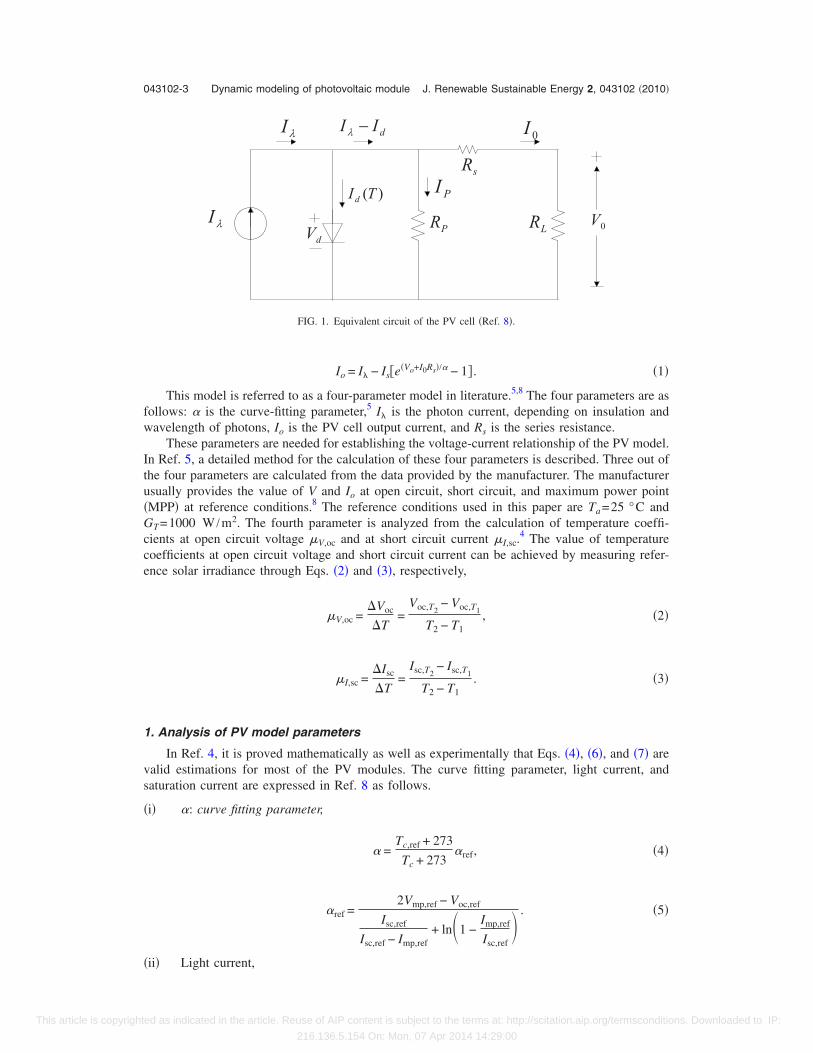
The basic criteria for modeling a PV device are its electrical characteristics, i.e., the currentnd voltage-current relationship of a PV cell for varying weather conditions.4,8 The equivalentlectrical circuit drawn in Fig. 1 is widely used in literature for the modeling of PV cells, whichs based on the finding of various researchers.4,5,8,14 This model is used for the modeling of a PV

odule and an array, depending on the number of cells connected in series in a module and theumber of modules connected in series or parallel in an array.

The values of these currents and voltages are dependent on the solar irradiance and thembient temperature.5,8,14 The relationship between the output voltage Vo and the load current Io is
elated as

216.136.5.154 On: Mon, 07 Apr 2014 14:29:00

fw

Itu�Gcce

1

vs

�

�

043102-3 Dynamic modeling of photovoltaic module J. Renewable Sustainable Energy 2, 043102 �2010�


Io = I� − Is�e�Vo+I0Rs�/� − 1� . �1�

This model is referred to as a four-parameter model in literature.5,8 The four parameters are asollows: � is the curve-fitting parameter,5 I� is the photon current, depending on insulation andavelength of photons, Io is the PV cell output current, and Rs is the series resistance.

These parameters are needed for establishing the voltage-current relationship of the PV model.n Ref. 5, a detailed method for the calculation of these four parameters is described. Three out ofhe four parameters are calculated from the data provided by the manufacturer. The manufacturersually provides the value of V and Io at open circuit, short circuit, and maximum power pointMPP� at reference conditions.8 The reference conditions used in this paper are Ta=25 °C and

T=1000 W /m2. The fourth parameter is analyzed from the calculation of temperature coeffi-ients at open circuit voltage �V,oc and at short circuit current �I,sc.

4 The value of temperatureoefficients at open circuit voltage and short circuit current can be achieved by measuring refer-nce solar irradiance through Eqs. �2� and �3�, respectively,

�V,oc =�Voc

�T=

Voc,T2− Voc,T1

T2 − T1, �2�

�I,sc =�Isc

�T=

Isc,T2− Isc,T1

T2 − T1. �3�

. Analysis of PV model parameters

In Ref. 4, it is proved mathematically as well as experimentally that Eqs. �4�, �6�, and �7� arealid estimations for most of the PV modules. The curve fitting parameter, light current, andaturation current are expressed in Ref. 8 as follows.

i� �: curve fitting parameter,

� =Tc,ref + 273

Tc + 273�ref, �4�

�ref =2Vmp,ref − Voc,ref

Isc,ref

Isc,ref − Imp,ref+ ln�1 −

Imp,ref

Isc,ref� . �5�

dV

PI

0V

0I

LRPR

sR

λI

λI dII −λ

)(TId

FIG. 1. Equivalent circuit of the PV cell �Ref. 8�.

ii� Light current,


216.136.5.154 On: Mon, 07 Apr 2014 14:29:00

�

�

ttc2l

bt

qfct

tS

�icI1

tcav



I� =GT

GT,ref�I�,ref + �I,sc�Tc − Tc,ref�� . �6�

Both I�,ref and �I,sc can be obtained from the manufacturer data sheet.4

iii� Saturation current Is is calculated at the reference condition as4,8,14

Is = Is,ref�Tc,ref + 273/Tc + 273�3e�EgNs/q�ref�1−�Tc,ref+273�/�Tc+273�−�� 7�

Is,ref = I�,refe�−Voc,ref/�ref�. �8�

iv� The value of the series resistance is usually provided by the manufacturer. It has also beenestimated as4

Rs = �ref ln�1 − Imp,ref/Isc,ref� + Voc,ref − Vmp,ref/Imp,ref. �9�

Note that the above model is a static model derived under the assumptions of constant PVemperature, constant weather condition, and constant solar irradiance. This static model is a toolo obtain the ideal characteristic of a PV cell under normal operating temperature and weatheronditions �NOCT�, which is the temperature in a PV module when the ambient temperature Ta is0 °C, solar irradiance GT is 800 W /m2, wind speed 1 m/s, and the manufacturer data given initerature.8

Recalling Eq. �1�, it is observable that the exact solution of this transcendental equation cannote found for output current of PV using combination of elementary functions. Equation �1� is ofhe form

x = f�x�, x = I0. �10�

Thus, it can be inferred from Ref. 20 that the Newton–Raphson process has a second-order oruadratic convergence for such transcendental equations. This methodology can be implementedor algebraic as well as transcendental equations and is valid even if the roots of the equation areomplex.20 A MATLAB® code is written and embedded in the SIMULINK model of the PV module forhe implementation of Newton–Raphson method for achieving the MPP of the PV module.

In the following pages, the static model is summarized briefly with the results obtainedhrough SIMULINK model based on static conditions. For the verification of the performance ofIMULINK model, two different solvers, namely, ode45 �dormand-price� and ode23Bogacki–Shampine�,21 are used to verify the model and similar results were obtained through themplementation of both the solvers. The PV module considered here for the study and analysisonsists of 153 cells in series and has the following manufacturer parameters �as shown in Table�.8 Temperature of the cell is considered as 25 °C for varying irradiance case and irradiance as000 W /m2 for varying temperature case.

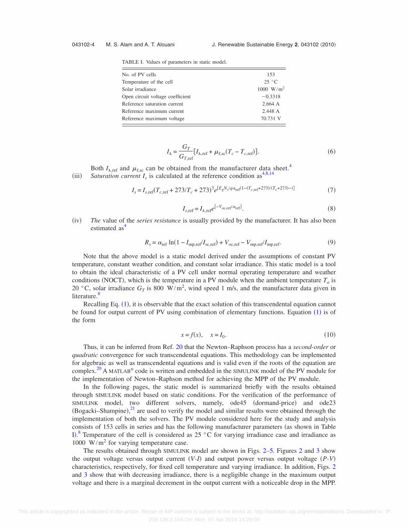
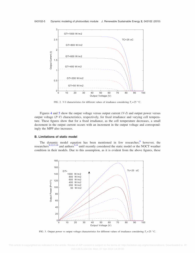
The results obtained through SIMULINK model are shown in Figs. 2–5. Figures 2 and 3 showhe output voltage versus output current �V-I� and output power versus output voltage �P-V�haracteristics, respectively, for fixed cell temperature and varying irradiance. In addition, Figs. 2nd 3 show that with decreasing irradiance, there is a negligible change in the maximum output

TABLE I. Values of parameters in static model.

No. of PV cells 153Temperature of the cell 25 °CSolar irradiance 1000 W /m2

Open circuit voltage coefficient �0.3318Reference saturation current 2.664 AReference maximum current 2.448 AReference maximum voltage 70.731 V

oltage and there is a marginal decrement in the output current with a noticeable drop in the MPP.


216.136.5.154 On: Mon, 07 Apr 2014 14:29:00

otdi

B

rc



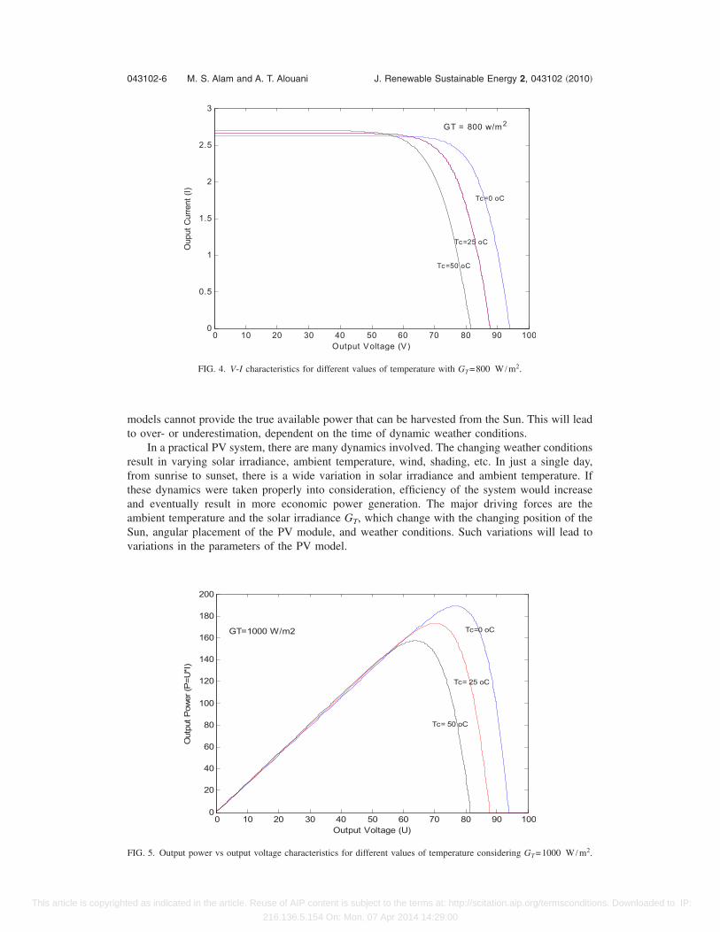
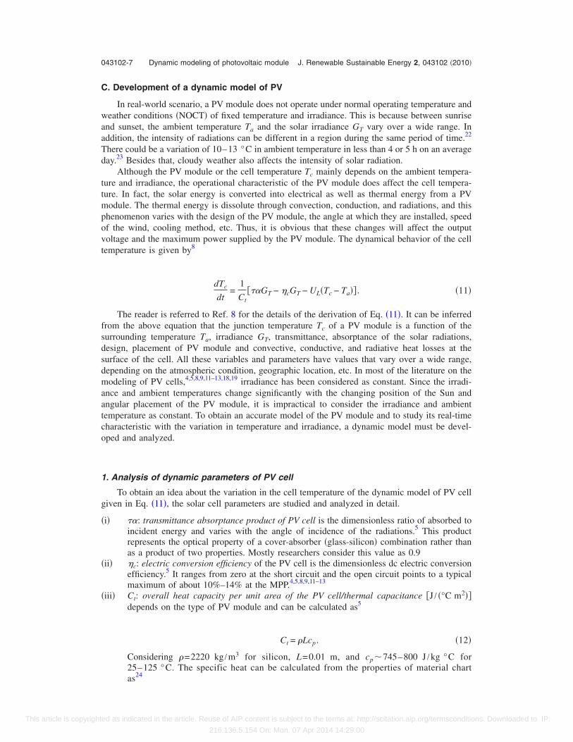
Figures 4 and 5 show the output voltage versus output current �V-I� and output power versusutput voltage �P-V� characteristics, respectively, for fixed irradiance and varying cell tempera-ure. These figures show that for a fixed irradiance, as the cell temperature decreases, a smallecrement in the output current occurs with an increment in the output voltage and correspond-ngly the MPP also increases.

. Limitations of static model

The dynamic model equation has been mentioned in few researches;8 however, theesearchers4,12,13,18 and authors5,14 until recently considered the static model or the NOCT weatherondition in their models. Due to this assumption, as it is evident from the above figures, these

0 10 20 30 40 50 60 70 80 90 1000

0.5

1

1.5

2

2.5

3

Output Voltage (V)

OutputCurrent(I)

GT=1000 W/m2

GT=800 W/m2

GT=600 W/m2

GT=400 W/m2

GT=200 W/m2

GT=50 W/m2

TC=25 oC

FIG. 2. V-I characteristics for different values of irradiance considering Tc=25 °C.

0 10 20 30 40 50 60 70 80 90 1000

20

40

60

80

100

120

140

160

180

Output Voltage (V)

OutputPower(P=V*I)

GT=1000 W /m2800 W /m2600 W /m2400 W /m2200 W /m250 W /m2

Tc=25 oC

FIG. 3. Output power vs output voltage characteristics for different values of irradiance considering Tc=25 °C.


216.136.5.154 On: Mon, 07 Apr 2014 14:29:00

mt

rftaaSv



odels cannot provide the true available power that can be harvested from the Sun. This will leado over- or underestimation, dependent on the time of dynamic weather conditions.

In a practical PV system, there are many dynamics involved. The changing weather conditionsesult in varying solar irradiance, ambient temperature, wind, shading, etc. In just a single day,rom sunrise to sunset, there is a wide variation in solar irradiance and ambient temperature. Ifhese dynamics were taken properly into consideration, efficiency of the system would increasend eventually result in more economic power generation. The major driving forces are thembient temperature and the solar irradiance GT, which change with the changing position of theun, angular placement of the PV module, and weather conditions. Such variations will lead toariations in the parameters of the PV model.

0 10 20 30 40 50 60 70 80 90 1000

0.5

1

1.5

2

2.5

3

Output Voltage (V)

OuputCurrent(I)

Tc=25 oC

Tc=50 oC

Tc=0 oC

GT = 800 w/m2

FIG. 4. V-I characteristics for different values of temperature with GT=800 W /m2.

0 10 20 30 40 50 60 70 80 90 1000

20

40

60

80

100

120

140

160

180

200

Output Voltage (U)

OutputPower(P=U*I)

GT=1000 W/m2

Tc= 50 oC

Tc= 25 oC

Tc=0 oC

2
FIG. 5. Output power vs output voltage characteristics for different values of temperature considering GT=1000 W /m .

216.136.5.154 On: Mon, 07 Apr 2014 14:29:00

C

waaTd

ttmpovt

fsdsdmaatco

1

g

�

�

�



. Development of a dynamic model of PV

In real-world scenario, a PV module does not operate under normal operating temperature andeather conditions �NOCT� of fixed temperature and irradiance. This is because between sunrise

nd sunset, the ambient temperature Ta and the solar irradiance GT vary over a wide range. Inddition, the intensity of radiations can be different in a region during the same period of time.22

here could be a variation of 10–13 °C in ambient temperature in less than 4 or 5 h on an averageay.23 Besides that, cloudy weather also affects the intensity of solar radiation.

Although the PV module or the cell temperature Tc mainly depends on the ambient tempera-ure and irradiance, the operational characteristic of the PV module does affect the cell tempera-ure. In fact, the solar energy is converted into electrical as well as thermal energy from a PV

odule. The thermal energy is dissolute through convection, conduction, and radiations, and thishenomenon varies with the design of the PV module, the angle at which they are installed, speedf the wind, cooling method, etc. Thus, it is obvious that these changes will affect the outputoltage and the maximum power supplied by the PV module. The dynamical behavior of the cellemperature is given by8

dTc

dt=

1

Ct��GT − �cGT − UL�Tc − Ta�� . �11�

The reader is referred to Ref. 8 for the details of the derivation of Eq. �11�. It can be inferredrom the above equation that the junction temperature Tc of a PV module is a function of theurrounding temperature Ta, irradiance GT, transmittance, absorptance of the solar radiations,esign, placement of PV module and convective, conductive, and radiative heat losses at theurface of the cell. All these variables and parameters have values that vary over a wide range,epending on the atmospheric condition, geographic location, etc. In most of the literature on theodeling of PV cells,4,5,8,9,11–13,18,19 irradiance has been considered as constant. Since the irradi-

nce and ambient temperatures change significantly with the changing position of the Sun andngular placement of the PV module, it is impractical to consider the irradiance and ambientemperature as constant. To obtain an accurate model of the PV module and to study its real-timeharacteristic with the variation in temperature and irradiance, a dynamic model must be devel-ped and analyzed.

. Analysis of dynamic parameters of PV cell

To obtain an idea about the variation in the cell temperature of the dynamic model of PV celliven in Eq. �11�, the solar cell parameters are studied and analyzed in detail.

i� ��: transmittance absorptance product of PV cell is the dimensionless ratio of absorbed toincident energy and varies with the angle of incidence of the radiations.5 This productrepresents the optical property of a cover-absorber �glass-silicon� combination rather thanas a product of two properties. Mostly researchers consider this value as 0.9

ii� �c: electric conversion efficiency of the PV cell is the dimensionless dc electric conversionefficiency.5 It ranges from zero at the short circuit and the open circuit points to a typicalmaximum of about 10%–14% at the MPP.4,5,8,9,11–13

iii� Ct: overall heat capacity per unit area of the PV cell/thermal capacitance �J / �°C m2��depends on the type of PV module and can be calculated as5

Ct = Lcp. �12�

Considering =2220 kg /m3 for silicon, L=0.01 m, and cp�745–800 J /kg °C for25–125 °C. The specific heat can be calculated from the properties of material chart

24
as

216.136.5.154 On: Mon, 07 Apr 2014 14:29:00

�

g

w�

w�

T

T

T

T

F

R



cp = AcdTc

dt. �13�

So, linearly interpolating the value of specific heat for 0–50 °C, Ct�1.6 e4 J / °C m2.iv� UL: overall heat loss coefficient is an overall �convective and radiative� loss coefficient,

with units of W /m2 C. For simplicity, the loss coefficient is assumed constant, whichneglects the effect of the factors, such as wind speed, humidity, and temperature, may haveon it.5 Although these factors may substantially affect the loss coefficient, their effect on theresulting absolute cell temperature is small.5,8 The detailed analysis is given below.

Overall heat loss coefficients,5

UL = Ut + Ub + Ue, �14�

ive bottom heat loss coefficient,

Ub = k1

L�15�

here k and L are the insulation thermal conductivity and thickness �k�0.045�. So, Ub

0.9 W /m2 C. Edge heat loss coefficient is given by5

Ue = kAe

A, �16�

here k is the insulation thermal conductivity �k�0.045�, Ae is the area of the edge, and so Ue

0.12 w /m2 C. Top heat loss coefficient is given by5

Ut = 1

hc,p−c + hr,p−c+

1

hw + hr,c−a−1

. �17�

he convective heat loss from plate to collector is5

hc,p−c = Nuk1

L. �18�

he radiation coefficient from plate to cover is5

hr,p−c =�Tp

2 + Tc2��Tp + Tc�

1

�p+

1

�c− 1

. �19�

he radiation coefficient from the cover to the air is5

hr,c−a = �c�Tc2 + Ta

2��Tc + Ta� . �20�

he wind heat loss coefficient5 is

hw = 2.8 + 3.0Vwind. �21�

rom Eq. �18�, hc,p−c=Nu�k1 /L�.The Nussle number is5

Nu = 1 + 1.441 −1708�sin 1.8��1.6

Ra cos �+1 −

1708

Ra cos �+

+ �Ra cos �

5830�1/3

− 1+

. �22�

5
eynolds number is given by

216.136.5.154 On: Mon, 07 Apr 2014 14:29:00

w�

T

T

a

T

I

C�cctt

2

E

w

E



Ra =g��TL3

�, �23�

here the difference in temperature of the cell/collector surface and temperature of the platebottom� is

�T = �Tp − Tc� . �24�

he volumetric coefficient of expansion �for an ideal gas� is

�� =1

Ta. �25�

herefore, Reynolds number will be5

Ra =gL3

��T

Ta� , �26�

nd Nussle number will be5

Nu = f��T

Ta,�� . �27�

herefore, the radiation coefficient between the plate and the cover will be5

hc,p−c =k1

Lf��T

Ta,�� . �28�

f the collector is installed at an angle of 60°, then

hc,p−c =k1

Lf��T

Ta� . �29�

onsidering as in Refs. 5 and 8: g=10 m /s2; �10−5, ��10−5; �p�0.95, �c�0.88; and L25 mm. For 0° �cos ��75°, consider Ta=25 °C and Tc=25 °C at GT=800 W /m2. UL is

alculated by writing a code in MATLAB® to obtain its range of variation. The range of heat lossoefficient obtained is 7.639�UL�8.468. This is in accordance with the literature.5,8 Consideringhe layer of glass over the silicon layer, the heat loss coefficient of glass will be calculated as thewo resistances in parallel.

. State space model of the dynamic PV model

A state space model is developed through the dynamic model �Eq. �11�� of the PV cell.quation �11� can be written as

dTc

dt= − b1Tc + b2Ta + aGT, �30�

here

a =1

Ct�� − �c� and b2 = − b1 =

1

Ct�UL� . �31�

quation �30� can be written in state space form as


216.136.5.154 On: Mon, 07 Apr 2014 14:29:00

C

w

I

scuatt

po8



Tc = − b1�Tc� + �b2 a��Ta

GT� . �32�

ompared with the state space model,

X = Ax + Bu ,

Y = Cx + Du , �33�

here

A = − b1, B = �b2 a1� ,

C = 1, D = 0. �34�

II. IMPLEMENTATION AND SIMULATION OF DYNAMIC MODEL IN SIMULINK

Ambient temperature Ta and the irradiance GT are the real-time variable inputs to the statepace model. The parameters a, b1, and b2 are calculated based on the standard values of the PVell parameters.8 The output of the state space model is the dynamic cell temperature, which issed to calculate the maximum voltage and maximum current of the PV cell to obtain the realisticvailable maximum power. Solar data have been collected from a weather station23,25 and analyzedhrough a SIMULINK model in the MATLAB® environment on a daily and monthly basis. For illus-ration purpose, data for a typical day of July 2005 �Refs. 23 and 25� have been considered.

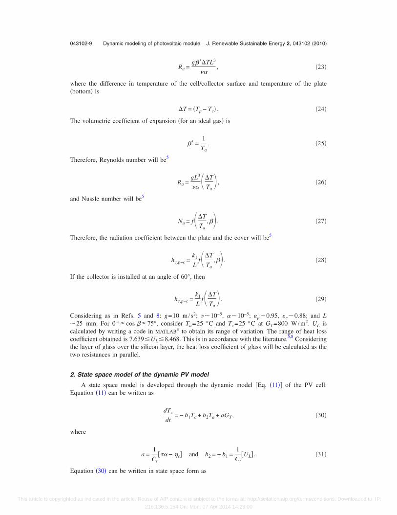
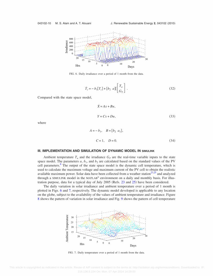
The daily variation in solar irradiance and ambient temperature over a period of 1 month islotted in Figs. 6 and 7, respectively. The dynamic model developed is applicable to any locationn the globe, subject to the availability of the values of ambient temperature and irradiance. Figureshows the pattern of variation in solar irradiance and Fig. 9 shows the pattern of cell temperature

!

" #

$

! !$

"

" %

& '

()*+,-+.--)/0)123

! "!#!

$!

%"!"%

#!

!

&!!'!!(!!#!!!)*

*+,-+./0

1*2 3+42

FIG. 6. Daily irradiance over a period of 1 month from the data.

!"#

! "

#

$

! !$

"

!$

"

"$

#

%&' () *(

+,-./013/,

4/*&15*/

$%&

%$'&

%$

'&

'$

(&

& &%&

'&(&

)*+#

,-./01230-40"*25"0

FIG. 7. Daily temperature over a period of 1 month from the data.


216.136.5.154 On: Mon, 07 Apr 2014 14:29:00

aiaal

atswta

I

dcpitmc



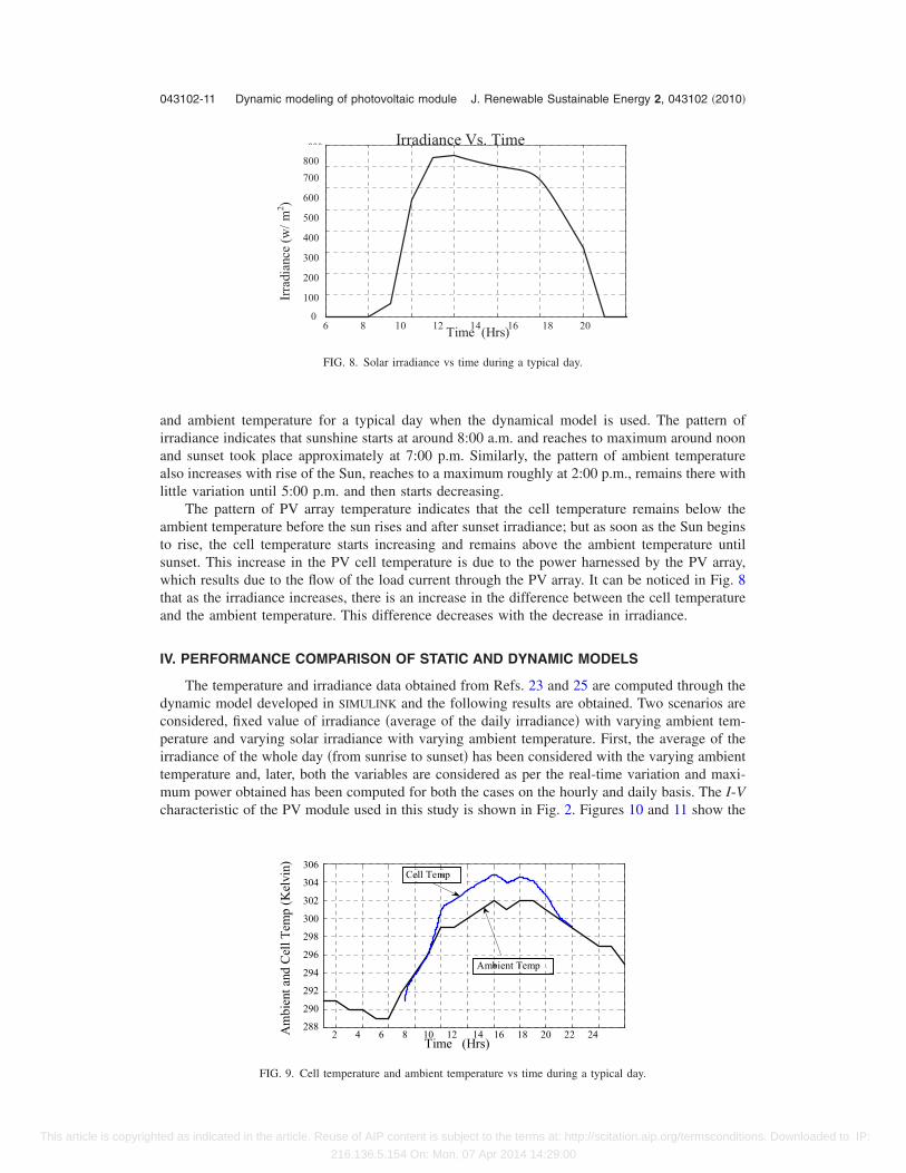
nd ambient temperature for a typical day when the dynamical model is used. The pattern ofrradiance indicates that sunshine starts at around 8:00 a.m. and reaches to maximum around noonnd sunset took place approximately at 7:00 p.m. Similarly, the pattern of ambient temperaturelso increases with rise of the Sun, reaches to a maximum roughly at 2:00 p.m., remains there withittle variation until 5:00 p.m. and then starts decreasing.

The pattern of PV array temperature indicates that the cell temperature remains below thembient temperature before the sun rises and after sunset irradiance; but as soon as the Sun beginso rise, the cell temperature starts increasing and remains above the ambient temperature untilunset. This increase in the PV cell temperature is due to the power harnessed by the PV array,hich results due to the flow of the load current through the PV array. It can be noticed in Fig. 8

hat as the irradiance increases, there is an increase in the difference between the cell temperaturend the ambient temperature. This difference decreases with the decrease in irradiance.

V. PERFORMANCE COMPARISON OF STATIC AND DYNAMIC MODELS

The temperature and irradiance data obtained from Refs. 23 and 25 are computed through theynamic model developed in SIMULINK and the following results are obtained. Two scenarios areonsidered, fixed value of irradiance �average of the daily irradiance� with varying ambient tem-erature and varying solar irradiance with varying ambient temperature. First, the average of therradiance of the whole day �from sunrise to sunset� has been considered with the varying ambientemperature and, later, both the variables are considered as per the real-time variation and maxi-

um power obtained has been computed for both the cases on the hourly and daily basis. The I-Vharacteristic of the PV module used in this study is shown in Fig. 2. Figures 10 and 11 show the

! " # " $ " % " " ! $ ##

" # #

$ # #

& # #

% # #

' # #

# #

( # #

! # #

) *+ , .*/ 0 12 3

41156*5/7,.8

92:;

+3

41 15 6 *5 / 7 , <2 ; ) *+ ,

!""#""

$""

%""

&""

'""

(""

)""

"$ ! )" )( )& )$ )! ("*+,- ./012

30045+467-.89,

( 2

30045+467- :1; *+,-

FIG. 8. Solar irradiance vs time during a typical day.

! " # $ % $ $ ! $ " $ # % ! # #

& %

&

& !

& "

& #

' % %

' %

' % !

' % "

( )* + - ). / 01 2

3*4)+.56

.78+99(

+*:-;+9<).2

8 + 9 9 (+ * : =

3 * 4 )+ . 5 ( + * : =!"#$%&' (%")

*%++ (%")

, - . / 01 0, 0- 0. 0/ ,1 ,, ,-($"% 23456

71.

71-

71,

711

,8/

,8.

,8-

,8,

,81

,//!"#$%&'9&:*%++(%")2;%+<$&6

FIG. 9. Cell temperature and ambient temperature vs time during a typical day.


216.136.5.154 On: Mon, 07 Apr 2014 14:29:00

pr

aatocfoi

9bSd

hf



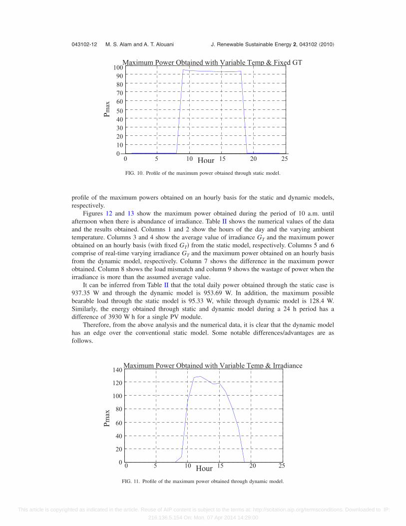
rofile of the maximum powers obtained on an hourly basis for the static and dynamic models,espectively.

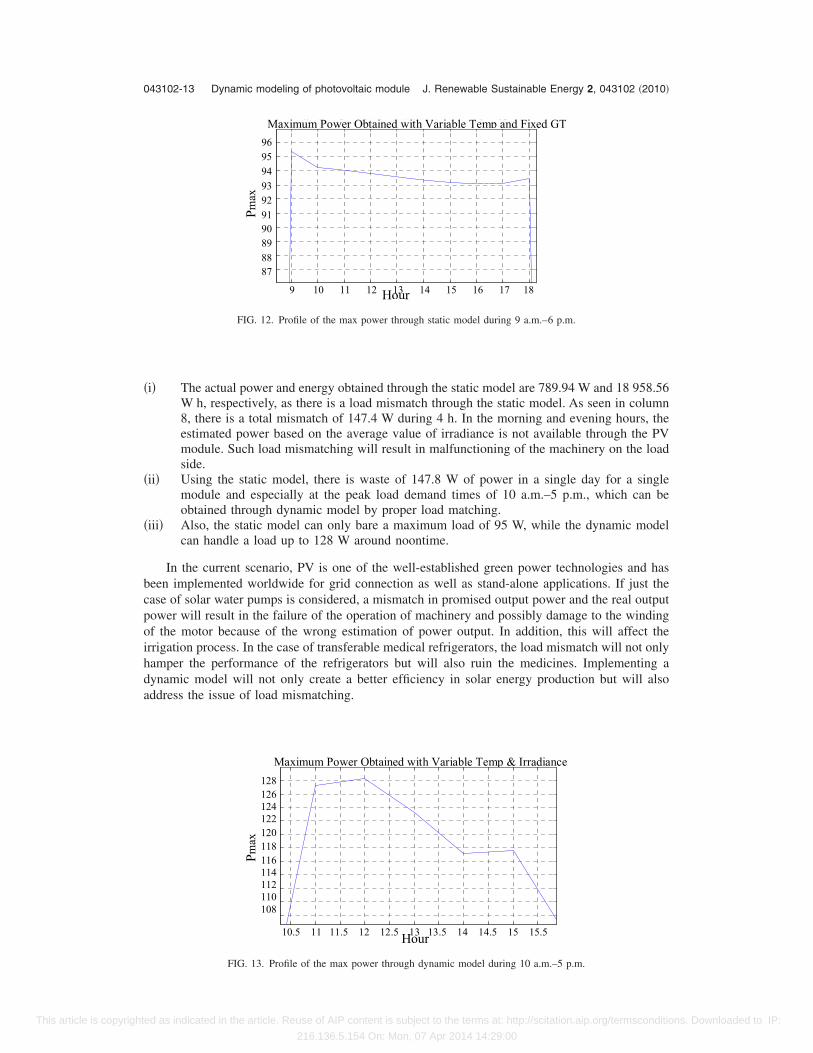
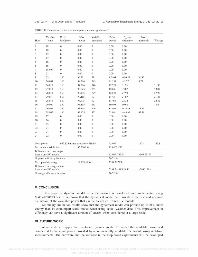
Figures 12 and 13 show the maximum power obtained during the period of 10 a.m. untilfternoon when there is abundance of irradiance. Table II shows the numerical values of the datand the results obtained. Columns 1 and 2 show the hours of the day and the varying ambientemperature. Columns 3 and 4 show the average value of irradiance GT and the maximum powerbtained on an hourly basis �with fixed GT� from the static model, respectively. Columns 5 and 6omprise of real-time varying irradiance GT and the maximum power obtained on an hourly basisrom the dynamic model, respectively. Column 7 shows the difference in the maximum powerbtained. Column 8 shows the load mismatch and column 9 shows the wastage of power when therradiance is more than the assumed average value.

It can be inferred from Table II that the total daily power obtained through the static case is37.35 W and through the dynamic model is 953.69 W. In addition, the maximum possibleearable load through the static model is 95.33 W, while through dynamic model is 128.4 W.imilarly, the energy obtained through static and dynamic model during a 24 h period has aifference of 3930 W h for a single PV module.

Therefore, from the above analysis and the numerical data, it is clear that the dynamic modelas an edge over the conventional static model. Some notable differences/advantages are asollows.

0 5 1 0 1 5 2 0 2 50

1 0

2 0

3 0

4 0

5 0

6 0

7 0

8 0

9 0

1 0 0M a x im um P o w e r O b t a in e d w i t h V a r ia b le t e m p a n d fix e d G T

H o u r

Pmax

0 5 10 15 20 25Hour

1009080706050403020100

Pmax

Maximum Power Obtained with Variable Temp & Fixed GT

FIG. 10. Profile of the maximum power obtained through static model.

0 5 10 1 5 20 2 50

20

40

60

80

1 00

1 20

1 40

H ou r

Pmax

M a x im um pow e r o b ta in ed w ith V a ria b le tem pe ra tu re a nd Irra d ia n c e

0 5 10 15 20 25Hour

140

120

100

80

60

40

20

0

Pmax

Maximum Power Obtained with Variable Temp & Irradiance

FIG. 11. Profile of the maximum power obtained through dynamic model.


216.136.5.154 On: Mon, 07 Apr 2014 14:29:00

�

�

�

bcpoihda



i� The actual power and energy obtained through the static model are 789.94 W and 18 958.56W h, respectively, as there is a load mismatch through the static model. As seen in column8, there is a total mismatch of 147.4 W during 4 h. In the morning and evening hours, theestimated power based on the average value of irradiance is not available through the PVmodule. Such load mismatching will result in malfunctioning of the machinery on the loadside.

ii� Using the static model, there is waste of 147.8 W of power in a single day for a singlemodule and especially at the peak load demand times of 10 a.m.–5 p.m., which can beobtained through dynamic model by proper load matching.

iii� Also, the static model can only bare a maximum load of 95 W, while the dynamic modelcan handle a load up to 128 W around noontime.

In the current scenario, PV is one of the well-established green power technologies and haseen implemented worldwide for grid connection as well as stand-alone applications. If just thease of solar water pumps is considered, a mismatch in promised output power and the real outputower will result in the failure of the operation of machinery and possibly damage to the windingf the motor because of the wrong estimation of power output. In addition, this will affect therrigation process. In the case of transferable medical refrigerators, the load mismatch will not onlyamper the performance of the refrigerators but will also ruin the medicines. Implementing aynamic model will not only create a better efficiency in solar energy production but will alsoddress the issue of load mismatching.

! " ! ! ! # ! $ !% !& !' !( !)

)(

))

)

"

!

#

$

%

&

'

* + , -. /. 1 23 45 6 7 8+ -94 : 3 -8; < + 5-+ 7 =4 84. > +9 : ?-, 4: @ A

B 2/ 5

1.+,

! "# "" "$ "% "& "' "( ") "*+,-.

!(!'!&!%!$!"!#*!***)

/0123-3 4,56. 78902:6; 529< =0.208>6 ?63@ 0:; A216; B?

4301

FIG. 12. Profile of the max power through static model during 9 a.m.–6 p.m.

! "# "# $ $ " # % % " # & & " # # # "#

! '

!

$

&

(

'

$ !

$ $

$ &

$ (

$ '

) * + ,

-./0

1 / 0 2. +. 4 * 5 6 , * 7 8/ 29 6 : 5 28 ; < / , 2/ 7 =6 8 6 . 4 6 ,/ 8 + ,6 / 9 : >,,/ : 2/ 9 ? 6

!"#$ !! !!#$ !% !%#$ !& !&#$ !' !'#$ !$ !$#$()*+

!%,!%-!%'!%%!%"!!,!!-!!'!!%!!"!",

./01

2013/*/ .)45+ 6780395: 438; <0+307=5 >5/? @ A++0:309B5

FIG. 13. Profile of the max power through dynamic model during 10 a.m.–5 p.m.


216.136.5.154 On: Mon, 07 Apr 2014 14:29:00

V

M

e

ee

V

cm

T

H

1

2

3

4

5

6

7

8

9

1

1

1

1

1

1

1

1

1

1

2

2

2

2

2

T

M

Df

%

M

Df

%



. CONCLUSION

In this paper, a dynamic model of a PV module is developed and implemented usingATLAB®/SIMULINK. It is shown that the dynamical model can provide a realistic and accurate

stimation of the available power that can be harnessed from a PV module.Preliminary simulation results show that the dynamical model can provide up to 21% more

nergy than its counterpart static model when using actual weather data. This improvement infficiency can save a significant amount of energy when considered at a large scale.

I. FUTURE WORK

Future work will apply the developed dynamic model to predict the available power andompare it to the actual power provided by a commercially available PV module using real-time

ABLE II. Comparison of the maximum power and energy obtained.

ourVariable

tempFixedirradiance

Maxpower

Variableirradiance

Maxpower

P_maxdifference

Loadmismatch Wastage

18 0 0.00 0 0.00 0.00

18 0 0.00 0 0.00 0.00

17 0 0.00 0 0.00 0.00

17 0 0.00 0 0.00 0.00

16 0 0.00 0 0.00 0.00

16 0 0.00 0 0.00 0.00

18.999 0 0.00 0 0.00 0.00

21 0 0.00 0 0.00 0.00

23 560 95.33 59 8.5108 �86.82 86.82

0 26.007 560 94.216 545 91.558 �3.77 3.77

1 26.011 560 94.216 746 127.29 31.96 31.96

2 27.011 560 93.845 755 128.4 33.07 33.07

3 28.011 560 93.475 729 123.31 27.98 27.98

4 29.01 560 93.105 697 117.2 21.87 21.87

5 28.011 560 93.475 697 117.65 22.32 22.32

6 29.009 560 93.105 633 105.93 10.60 10.6

7 29.007 560 93.104 496 81.897 �13.43 13.43

8 28.005 560 93.475 322 51.94 �43.39 43.39

9 27 0 0.00 0 0.00 0.00

0 26 0 0.00 0 0.00 0.00

1 25 0 0.00 0 0.00 0.00

2 24 0 0.00 0 0.00 0.00

3 24 0 0.00 0 0.00 0.00

4 22 0 0.00 0 0.00 0.00

otal power 937.35 but true available=789.94 953.69 147.41 147.8

aximum possible load 95.3300 W 128.4005 W

ifference in power outputrom a one PV module 953.69–789.94 =163.75 W

power efficiency increase 20.72 %

ax. possible energy 18 958.56 W h 2288.56 W h

ifference in energy outputrom a one PV module 2288.56–18 958.56 =3930 W h

energy efficiency increase 20.72 %

easurements. The hardware and the software in the loop-based experiments will be developed


216.136.5.154 On: Mon, 07 Apr 2014 14:29:00

fr�rdcd

NIIIIIIIIIIVVVVVVTTT��G��R��CULAcENkq



or comparison purpose. The SIMULINK model will be embedded into LABORATORY VIEW® envi-onment and the weather data will be obtained on a real-time basis through the data acquisitionDAQ� system. A thermocouple and an irradiance meter will be connected to DAQ to obtain theeal-time values of ambient temperature and irradiance. The predicted load value through theynamic model will be verified simultaneously on a commercial PV module. Further, intelligentontrol algorithm will be developed to implement the robust load matching as predicted by theynamic model.

omenclature� Photon current �A�s Reverse saturated current of the diode �A�d Temperature-dependent diode current �A�P PV cell leakage current �A�o PV cell output current �A�sc Short circuit current �A�mp,ref Maximum power point current at the reference condition �A�sc,ref Short circuit current at the reference condition �A�s,ref Saturation current at the reference condition �A��,ref Light current at the reference condition �A�o Output voltage �V�T Equivalent voltage to the junction temperature; VT=kT /q=T /11 �V�d Voltage across the diode �V�oc Open circuit voltage �V�oc,ref Open circuit voltage of the PV module at reference condition �V�mp,ref Maximum power point voltage at the reference condition �V�c PV cell temperature �°C�c,ref Reference temperature �°C�1, T2 Two temperatures centered on the reference temperature �°C�V,oc Temperature coefficients at open circuit voltage �V / °C�I,sc Temperature coefficient of the short-circuit current �Amp / °C�I,sc Temperature coefficient of the short-circuit current �Amp / °C�T, Graf Irradiance �W /m2�; reference irradiance �1000 W /m2�

Curve fitting parameter

ref The value of � at the reference condition �1000 W /m2 and 25 °C�s, Rp, RL Series resistance, shunt resistance, load resistance �� Transmittance-absorptance product of PV cell

c Electric conversion efficiency of the PV cell

t Overall heat capacity per unit area of the PV cell/thermal cap �J / �°F m2��L Overall heat loss coefficient �W /m2�

Density of the material �kg /m3�Thickness of the cell �m�Area of the PV Module �m2�

p Specific heat of silicon �J / °C m2�g Band gap of the material ��1.17 eV for Si materials�s Number of cells in series of a PV module

Boltzmann constant: k=1.380 47�10−23

Electron charge, q=1.602 10�10−19

1 J. A. Roger, Sol. Energy 23, 193 �1979�.2 M. Buresch, Photovoltaic Energy Systems Design and Installation �McGraw-Hill, New York, 1983�.3 G. J. Shushnar, J. H. Caldwell, R. F. Reinoehl, and J. H. Wilson, IEEE Trans. Power Appar. Syst. PAS-104, 2006 �1985�.4 T. U. Townsend, “A method for estimating the long-term performance of direct-coupled photovoltaic systems,” MSthesis, University of Wisconsin-Madison, 1989.

5
J. Duffie and W. A. Bechman, Solar Engineering of Thermal Processes �Wiley, New York, 1991�.

216.136.5.154 On: Mon, 07 Apr 2014 14:29:00

http://dx.doi.org/10.1016/0038-092X(79)90157-9

http://dx.doi.org/10.1109/TPAS.1985.318774

1

1

1

1

1

1

1

1

1

1

2

2

2

2

2

2



6 R. Bhide and S. R. Bhat, Proceedings of the 23rd Annual IEEE Power Electronics Specialization Conference, 1992, pp.708–713.

7 J. G. Vera, IEEE Trans. Energy Convers. 7, 426 �1992�.8 Ø. Ulleberg, “Stand-alone power systems for the future: Optimal design, operation and control of solar hydrogensystem,” Ph.D. thesis, NUST, 1998.

9 N. Mutoh, T. Matuo, K. Okada, and M. Sakai, Proceedings of the 33rd Annual IEEE Power Electronics SpecializationConference, 2002, pp. 1489–1494.

0 M. Bosanac, B. Sørensen, I. Katic, H. Sørensen, B. Nielsen, and J. Badran, “Photovoltaic/thermal solar collectors andtheir potential in Denmark,” EFP Report No. 1713/00-0014, May 2003.

1 C. Chiang, T.-S. Chiang, and H.-S. Huang, Proceedings of the Third World Conference on Photovoltaic Energy Conver-sion, Osaka, Japan, 11–18 May 2003.

2 Y. T. Tan, IEEE Trans. Energy Convers. 19, 748 �2004�.3 A. D. Theocharis, A. Menti, J. Milias-Argitis, T. Zacharias, Power Tech, 2005 IEEE, Russia, 27–30 June 2005.4 F. Ferret and M. Godoy Simões, Integration of Alternative Sources of Energy �Wiley, New York, 2006�.5 U. Paatero and P. D. Lund, Renewable Energy 32, 216 �2007�.6 T. Esram and P. L. Chapman IEEE Trans. Energy Convers. 22, 439 �2007�.7 R. Chenni, M. Makhlouf, T. Kerbache, and A. Bouzid, J. Energy 32, 1724 �2007�.8 A. Mellit and S. A. Kalogirou, Progress in Energy and Combustion Science 34, 574 �2008�.9 A. Al-Alawi, S. M. Al-Alawi, and S. M. Islam, Renewable Energy 32, 1426 �2007�.0 S. S. Sastry, Introductory Methods of Numerical Analysis, 4th ed. �PHI, India, 2006�.1

MATLAB/SIMULINK, as in MATLAB version 7.0 �http://www.mathworks.com�.2 J. F. Randall and J. Jacot, Renewable Energy 28, 1851 �2003�.3 National Solar Radiation Database, http://rredc.nrel.gov/solar/old_data/nsrdb/, accessed on December 4, 2008.4 F. P. Incropera, D. P. Dewitt, T. L. Bergman, and A. S. Laving, Fundamentals of Heat and Mass Transfer, 6th ed. �Wiley,New York, 2006�.

5 NOAA National Climatic Data Center, ftp.ncdc.noaa.gov, accessed on May 1, 2009.


216.136.5.154 On: Mon, 07 Apr 2014 14:29:00

http://dx.doi.org/10.1109/60.148562

http://dx.doi.org/10.1109/TEC.2004.827707

http://dx.doi.org/10.1016/j.renene.2006.01.005

http://dx.doi.org/10.1109/TEC.2006.874230

http://dx.doi.org/10.1016/j.energy.2006.12.006

http://dx.doi.org/10.1016/j.pecs.2008.01.001

http://dx.doi.org/10.1016/j.renene.2006.05.003

http://www.mathworks.com

http://dx.doi.org/10.1016/S0960-1481(03)00068-5

http://rredc.nrel.gov/solar/old_data/nsrdb/

ftp.ncdc.noaa.gov

Documents

Dynamic modeling of photovoltaic module for real-time maximum power tracking