Dynamic Snap-Through of Thermally Buckled Structures

by a Reduced Order Method

Adam Przekop*

National Institute of Aerospace, Hampton, VA 23666

Stephen A. Rizzi†

NASA Langley Research Center, Hampton, VA 23681

The goal of this investigation is to further develop nonlinear modal numerical simulation methods for

application to geometrically nonlinear response of structures exposed to combined high intensity random

pressure fluctuations and thermal loadings. The study is conducted on a flat aluminum beam, which permits

a comparison of results obtained by a reduced-order analysis with those obtained from a numerically

intensive simulation in physical degrees-of-freedom. A uniformly distributed thermal loading is first applied

to investigate the dynamic instability associated with thermal buckling. A uniformly distributed random

loading is added to investigate the combined thermal-acoustic response. In the latter case, three types of

response characteristics are considered, namely: (i) small amplitude vibration around one of the two stable

buckling equilibrium positions, (ii) intermittent snap-through response between the two equilibrium

positions, and (iii) persistent snap-through response between the two equilibrium positions. For the reduced-

order analysis, four categories of modal basis functions are identified including those having symmetric

transverse, anti-symmetric transverse, symmetric in-plane, and anti-symmetric in-plane displacements. The

effect of basis selection on the quality of results is investigated for the dynamic thermal buckling and

combined thermal-acoustic response. It is found that despite symmetric geometry, loading, and boundary

conditions, the anti-symmetric transverse and symmetric in-plane modes must be included in the basis as they

participate in the snap-through behavior.

* Research Scientist, AIAA Senior Member. † Aerospace Engineer, Structural Acoustics Branch, AIAA Associate Fellow.

1

https://ntrs.nasa.gov/search.jsp?R=20070034829 2018-07-07T07:01:10+00:00Z

Nomenclature

,M M = mass matrix (physical and modal coordinates)

,C C = proportional damping matrix (physical and modal coordinates)

,K K = stiffness matrix (physical and modal coordinates)

,X q = displacement response vector (physical and modal coordinates)

,F F = force excitation vector (physical and modal coordinates)

, NL NLF F = nonlinear restoring force (physical and modal coordinates)

F = modal basis function matrix

, ,u v f = horizontal and vertical displacement, and rotation (global physical coordinates)

TD = temperature increment

t = time

, ,d a b = linear, quadratic nonlinear, and cubic nonlinear modal stiffness coefficients

È ˚Ι = identity matrix

a = thermal expansion coefficient

z = viscous damping factor

w = undamped natural frequencies

I. Introduction

IRECT numerical simulation of nonlinear random response in physical degrees-of-freedom (DoF) is

computationally intensive even for the simplest structures. Its use for design of high-cycle-fatigue tolerant

aerospace vehicle structures, requiring long simulation times to obtain meaningful statistics, is considered

impractical. Accordingly, much effort has been spent in recent years to develop accurate reduced-order analyses,

such as finite-element-based nonlinear modal numerical simulation, which could be suitable for use in design

environments.

D

Aerospace structures exposed to a high-intensity random acoustic loading are often also simultaneously exposed

to an elevated thermal environment.1 Since both acoustic and thermal loadings can cause the structure to respond in

2

a geometrically nonlinear fashion, an analysis technique that permits simultaneous loading is required, i.e. linear

superposition of the acoustic and thermal response is not suitable. Under certain thermal-acoustic loading

conditions, experimental studies indicate a snap-though response,2-4 which can significantly reduce fatigue life. The

snap-through problem has previously been investigated using reduced-order analyses with both closed-form5-11 and

finite element (FE)12-15 solutions. Reduced-order FE analysis can be further classified into so-called direct12-14 and

indirect15 stiffness evaluation procedure approaches. For both direct and indirect approaches, the system is first

transformed to a reduced set of coupled nonlinear equations, which are solved via numerical integration. Since the

eventual application is the analysis and design of practical structures, this paper focuses on developments associated

with the indirect approach, which has been implemented for use with commercial finite element codes.15-17 The

previous work15 using the indirect procedure modeled the dynamic snap-through response with a single transverse

mode. However, it has been subsequently shown that a significant improvement can be obtained using a basis

consisting of both low-frequency transverse-dominated modes and high-frequency in-plane-dominated modes.17,18

The present work concentrates on selecting such a basis so that both the transverse and in-plane dynamic behaviors

of the system can be accurately modeled.

A clamped-clamped aluminum beam is considered in this work to allow reduced-order analysis results to be

compared with a numerically intensive simulation in physical DoF. The dynamic thermal buckling problem is first

studied by applying a uniformly distributed, positive temperature increment. The combined thermal-acoustic

loading is subsequently investigated through the addition of uniformly distributed acoustic loadings of different

intensities. Several response characteristics are investigated including: (i) small amplitude vibration around one of

two stable, buckled equilibrium positions, (ii) intermittent snap-through response between the two buckled

equilibrium positions, and (iii) persistent snap-through response between the two buckled equilibrium positions. In

each case, the reduced-order analysis is performed with two different sets of basis functions, and results are

compared with those obtained by numerical simulation in physical DoF.

II. Reduced-Order Numerical Simulation

The reduced-order analysis is first presented as it is used to study the response to both thermal and thermal-

acoustic loadings. Similarities between the direct and indirect stiffness evaluation methods are discussed.

A. Modal Coordinate Transformation

3

In the direct stiffness evaluation approach, the equations of motion for a nonlinear system subjected to a change

in temperature can be expressed in the form12-14

( ) ( )1 2( ) ( ) ( ) ( ) ( ), ( ) ( ) ( )Tt t K K T K t K t t t t∆ ∆⎡+ + − ∆ + + = +⎣ ⎤⎦L TMX CX X X X X F F (1)

where M is the mass matrix, C is the mass proportional damping matrix (no temperature dependence is assumed),

and , , and are the linear, quadratic, and cubic stiffness matrices, respectively. X is the displacement

response vector and F is the force excitation vector. The thermal effect is present on both sides of Eq. (1); as a

change in the linear stiffness matrix on the left-hand-side, and as a thermal force vector

KL 1K 2K

(TK T∆ ∆ ) ∆TF on the right-

hand-side.

In the indirect stiffness evaluation approach, the equation of motion is written in the form

(2) ( ) ( ) ( ( ), ) ( )t t t T+ + ∆ =NLMX CX F X F t

Here, the thermal effect is represented entirely on the left-hand-side of the equation in the nonlinear restoring force

NLF , which also contains the linear, quadratic and cubic stiffness terms. Comparing Eqs. (1) and (2), a relationship

between direct and indirect formulations is established, namely,

( ) ( )1 2( ( ), ) ( ) ( ) ( ), ( ) ( )Tt T K K T K t K t t t∆ ∆⎡∆ = − ∆ + +⎣NL L T⎤⎦F X X X X X - F (3)

Continuing with the indirect approach, a set of coupled modal equations with reduced DoF is obtained by

applying the modal coordinate transformation =X qF to Eq. (2), where q is the modal displacement response

vector. In this study, the set of modal basis functions, , is formed from the linear eigenvalue problem using only

that part of the restoring force associated with the linear stiffness, without the effect of temperature. These are

sometimes referred to as “cold modes.” Generally, a small set of L basis functions is included resulting in a modal

equation of motion that takes the form

F

(4) 1 2( ) ( ) ( ( ), ( ), , ( ), ) ( )Lt t q t q t q t T+ + ∆ =…NLMq Cq F F t

T F

The tilde superscript represents modal quantities, and

. (5) 2T T Tr r NL NLζ ω= ⎡ ⎦ = = ⎡ ⎦ = =M M I C C F F FΦ Φ = Φ Φ Φ Φ

B. Indirect Stiffness Evaluation Method

4

The previously developed15-17 indirect stiffness evaluation procedure is used. To summarize, the r-th element of

the nonlinear restoring force vector in Eq. (4) can be formed by computing

( )1 21 1 1

( , , , , ) 1,2, ,L L L L L L

r r r rNL L j j jk j k jkl j k l

j j k j j k j l kF q q q T d T q a q q b q q q r L

= = = = = =

∆ = ∆ + + =∑ ∑∑ ∑∑∑… … (6)

where d, a, and b are the linear, quadratic nonlinear, and cubic nonlinear modal stiffness coefficients, respectively.

The indirect stiffness evaluation procedure reduces the problem of determining the nonlinear modal stiffness to a

series of static nonlinear problems with prescribed displacement fields and, if required, temperatures. The

prescribed displacement fields are formed from combinations of modes in the basis. Once the resulting nonlinear

forces are determined, the nonlinear modal stiffness coefficients may be found by solution of a simple algebraic

system of equations. Note that the thermal loading can have an arbitrary spatial and through-the-thickness

distribution, as long as such a distribution is supported by a commercial FE code used to compute the nonlinear

restoring forces.

C. Implementation

The program RANSTEP was used to perform the reduced-order analysis with the indirect stiffness evaluation

procedure. In particular, the RANSTEP implementation for MSC.NASTRAN was used because of successful

application to similar problems.17 The implementation consists of several steps. The linear eigenvectors are first

obtained from a normal modes analysis (Solution 103). The required displacement fields are then formed as a

summation of selected and appropriately scaled basis functions. Next, a series of static nonlinear solutions (Solution

106) are performed at a prescribed elevated temperature to obtain the corresponding restoring forces. Based on

these forces, the modal stiffness coefficients are evaluated. The resulting coupled system of equations, Eq. (4), is

numerically integrated using the fourth order Runge-Kutta scheme to obtain a modal displacement time history. An

inverse modal transformation allows the physical displacement to be computed.

D. Finite Element Model

The beam under analysis measured 18-in. x 1-in. x 0.09-in (length x width x thickness). The FE model consisted

of 144 CBEAM beam elements, each measuring 0.125-in. in length. Clamped boundary conditions were applied at

both ends of the beam by specifying zero displacement and rotation. The following material properties were used:

5

6 6 42

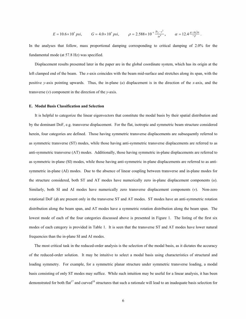
410.6 10 , 4.0 10 , 2.588 10 12.4,flb s in inFin

E psi G psi µρ α− − −°

= × = × = × = .

In the analyses that follow, mass proportional damping corresponding to critical damping of 2.0% for the

fundamental mode (at 57.8 Hz) was specified.

Displacement results presented later in the paper are in the global coordinate system, which has its origin at the

left clamped end of the beam. The x-axis coincides with the beam mid-surface and stretches along its span, with the

positive y-axis pointing upwards. Thus, the in-plane (u) displacement is in the direction of the x-axis, and the

transverse (v) component in the direction of the y-axis.

E. Modal Basis Classification and Selection

It is helpful to categorize the linear eigenvectors that constitute the modal basis by their spatial distribution and

by the dominant DoF, e.g. transverse displacement. For the flat, isotropic and symmetric beam structure considered

herein, four categories are defined. Those having symmetric transverse displacements are subsequently referred to

as symmetric transverse (ST) modes, while those having anti-symmetric transverse displacements are referred to as

anti-symmetric transverse (AT) modes. Additionally, those having symmetric in-plane displacements are referred to

as symmetric in-plane (SI) modes, while those having anti-symmetric in-plane displacements are referred to as anti-

symmetric in-plane (AI) modes. Due to the absence of linear coupling between transverse and in-plane modes for

the structure considered, both ST and AT modes have numerically zero in-plane displacement components (u).

Similarly, both SI and AI modes have numerically zero transverse displacement components (v). Non-zero

rotational DoF (φ) are present only in the transverse ST and AT modes. ST modes have an anti-symmetric rotation

distribution along the beam span, and AT modes have a symmetric rotation distribution along the beam span. The

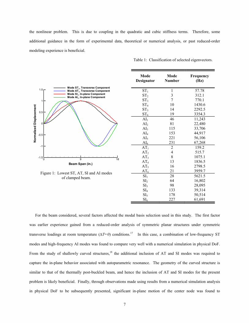
lowest mode of each of the four categories discussed above is presented in Figure 1. The listing of the first six

modes of each category is provided in Table 1. It is seen that the transverse ST and AT modes have lower natural

frequencies than the in-plane SI and AI modes.

The most critical task in the reduced-order analysis is the selection of the modal basis, as it dictates the accuracy

of the reduced-order solution. It may be intuitive to select a modal basis using characteristics of structural and

loading symmetry. For example, for a symmetric planar structure under symmetric transverse loading, a modal

basis consisting of only ST modes may suffice. While such intuition may be useful for a linear analysis, it has been

demonstrated for both flat17 and curved18 structures that such a rationale will lead to an inadequate basis selection for

6

the nonlinear problem. This is due to coupling in the quadratic and cubic stiffness terms. Therefore, some

additional guidance in the form of experimental data, theoretical or numerical analysis, or past reduced-order

modeling experience is beneficial.

Beam Span (in.)

Nor

mal

ized

Dis

plac

emen

t

0 9-1.5

-1

-0.5

0

0.5

1

1.5Mode ST1, Transverse ComponentMode AT1, Transverse ComponentMode SI1, In-plane ComponentMode AI1, In-plane Component

18

Figure 1: Lowest ST, AT, SI and AI modes of clamped beam.

Table 1: Classification of selected eigenvectors.

Mode Designator

Mode Number

Frequency (Hz)

ST1 1 57.78 ST2 3 312.1 ST3 7 770.1 ST4 10 1430.6 ST5 14 2292.5 ST6 19 3354.3 AI1 46 11,243 AI2 81 22,480 AI3 115 33,706 AI4 153 44,917 AI5 221 56,106 AI6 231 67,268 AT1 2 159.2 AT2 4 515.7 AT3 8 1075.1 AT4 13 1836.5 AT5 16 2798.5 AT6 21 3959.7 SI1 28 5621.5 SI2 64 16,802 SI3 98 28,095 SI4 133 39,314 SI5 178 50,514 SI6 227 61,691

For the beam considered, several factors affected the modal basis selection used in this study. The first factor

was earlier experience gained from a reduced-order analysis of symmetric planar structures under symmetric

transverse loadings at room temperature (∆T=0) conditions.17 In this case, a combination of low-frequency ST

modes and high-frequency AI modes was found to compare very well with a numerical simulation in physical DoF.

From the study of shallowly curved structures,18 the additional inclusion of AT and SI modes was required to

capture the in-plane behavior associated with autoparametric resonance. The geometry of the curved structure is

similar to that of the thermally post-buckled beam, and hence the inclusion of AT and SI modes for the present

problem is likely beneficial. Finally, through observations made using results from a numerical simulation analysis

in physical DoF to be subsequently presented, significant in-plane motion of the center node was found to

7

accompany the snap-through response, further substantiating the need for SI modes in the modal basis. While not

required for the simple beam, a Proper Orthogonal Decomposition (POD) analysis of data from an FE analysis in

physical DoF could provide guidance for more complicated structures.19,20

Thus, the modal basis chosen for this study consisted of all four types of modes. Based on the frequency range

of the excitation, the six lowest modes of each four types were used to establish the modal basis. In the discussion

that follows, this set will be referred to as the 24-mode basis. To explore the impact of selecting an insufficient basis

on the quality of the reduced-order results, a truncated basis was assembled from the six lowest ST modes and the

six lowest AI modes. This basis lacked the SI modes necessary to capture the in-plane motion at the beam center.

In the following, it will be referred to as the 12-mode basis.

F. Modal Stiffness Coefficients

The behavior of modal stiffness coefficients as a function of applied temperature increment was examined and

warrants a discussion. For the purpose of this investigation, modal stiffness coefficients were computed at room

temperature, and at two uniformly distributed temperature increments of 35°F and 70°F. There was no thermal

gradient through the thickness. Since the critical buckling temperature CRT∆ of the beam was found to be 6.6°F, the

two elevated temperature cases corresponded to approximately 5.3 and 10.6 times CRT∆ , respectively. Both the 12-

and 24-mode bases were used.

Examination of the nonlinear quadratic and cubic modal stiffness matrices revealed that they were not affected

by the temperature change. This observation is in agreement with the direct reduced order FE formulation, where

the nonlinear stiffness matrices are only a function of displacement, regardless of how this displacement was

induced.13,14 The linear modal stiffness coefficients however were found to be strongly dependent on the

temperature change. For the room temperature condition, the linear modal stiffness matrix is uncoupled. The linear

stiffness coefficients are the positive eigenvalues and equal to the square of the natural frequencies of the system.

Further, since the matrix is diagonal, the linear modal stiffness does not contribute to the overall coupling of

transverse and in-plane modes. At elevated temperatures, some of the off-diagonal stiffness terms become

significant, resulting in a coupled linear modal stiffness matrix. For both temperatures and bases considered, only

the portion of the linear matrix corresponding to the low-frequency transverse modes (ST in the 12-mode basis, and

ST and AT in the 24-mode basis) was altered. The off-diagonal terms were symmetric. These observations are also

8

consistent with the previous direct reduced order FE development.13,14 Moreover, in the case of the 12-mode basis,

the low-frequency portion of the linear stiffness was fully populated, effectively coupling all ST modes included in

the basis. In the case of the 24-mode basis, the coupling between ST modes was large, and the coupling between

AT modes was large, but no linear cross-coupling occurred between the ST and AT modes. These observations are

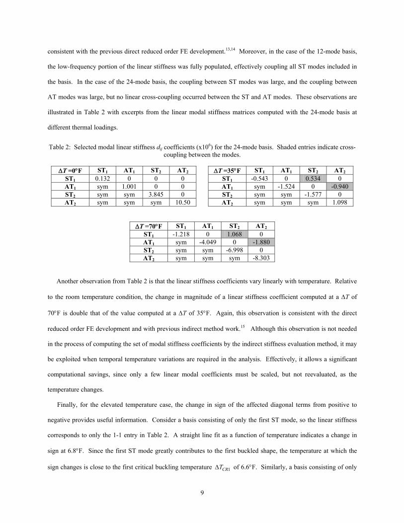
illustrated in Table 2 with excerpts from the linear modal stiffness matrices computed with the 24-mode basis at

different thermal loadings.

Table 2: Selected modal linear stiffness dij coefficients (x106) for the 24-mode basis. Shaded entries indicate cross-coupling between the modes.

∆T =0°F ST1 AT1 ST2 AT2

ST1 0.132 0 0 0 AT1 sym 1.001 0 0 ST2 sym sym 3.845 0 AT2 sym sym sym 10.50

∆T =35°F ST1 AT1 ST2 AT2

ST1 -0.543 0 0.534 0 AT1 sym -1.524 0 -0.940 ST2 sym sym -1.577 0 AT2 sym sym sym 1.098

∆T =70°F ST1 AT1 ST2 AT2

ST1 -1.218 0 1.068 0 AT1 sym -4.049 0 -1.880 ST2 sym sym -6.998 0 AT2 sym sym sym -8.303

Another observation from Table 2 is that the linear stiffness coefficients vary linearly with temperature. Relative

to the room temperature condition, the change in magnitude of a linear stiffness coefficient computed at a ∆T of

70°F is double that of the value computed at a ∆T of 35°F. Again, this observation is consistent with the direct

reduced order FE development and with previous indirect method work.15 Although this observation is not needed

in the process of computing the set of modal stiffness coefficients by the indirect stiffness evaluation method, it may

be exploited when temporal temperature variations are required in the analysis. Effectively, it allows a significant

computational savings, since only a few linear modal coefficients must be scaled, but not reevaluated, as the

temperature changes.

Finally, for the elevated temperature case, the change in sign of the affected diagonal terms from positive to

negative provides useful information. Consider a basis consisting of only the first ST mode, so the linear stiffness

corresponds to only the 1-1 entry in Table 2. A straight line fit as a function of temperature indicates a change in

sign at 6.8°F. Since the first ST mode greatly contributes to the first buckled shape, the temperature at which the

sign changes is close to the first critical buckling temperature 1CRT∆ of 6.6°F. Similarly, a basis consisting of only

9

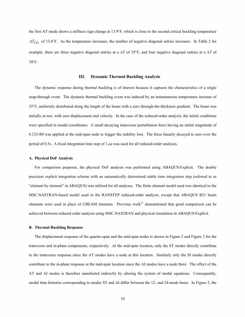
the first AT mode shows a stiffness sign change at 13.9°F, which is close to the second critical buckling temperature

of 13.6°F. As the temperature increases, the number of negative diagonal entries increases. In Table 2 for

example, there are three negative diagonal entries at a ∆T of 35°F, and four negative diagonal entries at a ∆T of

70°F.

2CRT∆

III. Dynamic Thermal Buckling Analysis

The dynamic response during thermal buckling is of interest because it captures the characteristics of a single

snap-through event. The dynamic thermal buckling event was induced by an instantaneous temperature increase of

35°F, uniformly distributed along the length of the beam with a zero through-the-thickness gradient. The beam was

initially at rest, with zero displacement and velocity. In the case of the reduced-order analysis, the initial conditions

were specified in modal coordinates. A small decaying transverse perturbation force having an initial magnitude of

0.125-lbf was applied at the mid-span node to trigger the stability loss. The force linearly decayed to zero over the

period of 0.5s. A fixed integration time step of 1 µs was used for all reduced-order analyses.

A. Physical DoF Analysis

For comparison purposes, the physical DoF analysis was performed using ABAQUS/Explicit. The double

precision explicit integration scheme with an automatically determined stable time integration step (referred to as

“element by element” in ABAQUS) was utilized for all analyses. The finite element model used was identical to the

MSC.NASTRAN-based model used in the RANSTEP reduced-order analysis, except that ABAQUS B21 beam

elements were used in place of CBEAM elements. Previous work17 demonstrated that good comparison can be

achieved between reduced order analysis using MSC.NASTRAN and physical simulation in ABAQUS/Explicit.

B. Thermal Buckling Response

The displacement response of the quarter-span and the mid-span nodes is shown in Figure 2 and Figure 3 for the

transverse and in-plane components, respectively. At the mid-span location, only the ST modes directly contribute

to the transverse response since the AT modes have a node at this location. Similarly only the SI modes directly

contribute to the in-plane response at the mid-span location since the AI modes have a node there. The effect of the

AT and AI modes is therefore manifested indirectly by altering the system of modal equations. Consequently,

modal time histories corresponding to modes ST and AI differ between the 12- and 24-mode bases. In Figure 2, the

10

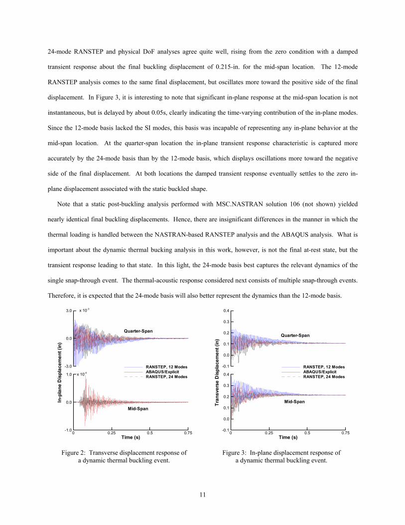
24-mode RANSTEP and physical DoF analyses agree quite well, rising from the zero condition with a damped

transient response about the final buckling displacement of 0.215-in. for the mid-span location. The 12-mode

RANSTEP analysis comes to the same final displacement, but oscillates more toward the positive side of the final

displacement. In Figure 3, it is interesting to note that significant in-plane response at the mid-span location is not

instantaneous, but is delayed by about 0.05s, clearly indicating the time-varying contribution of the in-plane modes.

Since the 12-mode basis lacked the SI modes, this basis was incapable of representing any in-plane behavior at the

mid-span location. At the quarter-span location the in-plane transient response characteristic is captured more

accurately by the 24-mode basis than by the 12-mode basis, which displays oscillations more toward the negative

side of the final displacement. At both locations the damped transient response eventually settles to the zero in-

plane displacement associated with the static buckled shape.

Note that a static post-buckling analysis performed with MSC.NASTRAN solution 106 (not shown) yielded

nearly identical final buckling displacements. Hence, there are insignificant differences in the manner in which the

thermal loading is handled between the NASTRAN-based RANSTEP analysis and the ABAQUS analysis. What is

important about the dynamic thermal bucking analysis in this work, however, is not the final at-rest state, but the

transient response leading to that state. In this light, the 24-mode basis best captures the relevant dynamics of the

single snap-through event. The thermal-acoustic response considered next consists of multiple snap-through events.

Therefore, it is expected that the 24-mode basis will also better represent the dynamics than the 12-mode basis.

-3.0

0.0

3.0

RANSTEP, 12 ModesABAQUS/ExplicitRANSTEP, 24 Modes

Mid-Span

Quarter-Span

x 10-3

Time (s)

In-p

lane

Dis

plac

emen

t(in

)

0 0.25 0.5 0.75-1.0

0.0

1.0 x 10-4

Figure 2: Transverse displacement response of a dynamic thermal buckling event.

Time (s)

Tran

sver

seD

ispl

acem

ent(

in)

0 0.25 0.5 0.75-0.1

0.0

0.1

0.2

0.3

0.4

-0.1

0.0

0.1

0.2

0.3

0.4

RANSTEP, 12 ModesABAQUS/ExplicitRANSTEP, 24 Modes

Mid-Span

Quarter-Span

Figure 3: In-plane displacement response of a dynamic thermal buckling event.

11

IV. Thermal-Acoustic Response Analysis

The dynamic response of the beam to a combined thermal-acoustic load was next investigated. The thermal load

was instantaneously applied to the beam via a uniformly distributed temperature increase of 35°F with a zero

through-the-thickness gradient. A Gaussian random pressure load with a flat excitation spectrum from 0-1500 Hz

was generated using a previously developed procedure.21 The frequency range of the pressure loading was lower

than the maximum frequency of the low frequency ST and AT modes. Almost half of those selected were outside

the excitation bandwidth, while all of the SI and AI modes resided significantly above the excitation bandwidth.

The pressure was uniformly applied along the span in the transverse direction, irrespective of the deformation, i.e.

follower forces were not utilized. Excitation levels of 128 dB, 158 dB, and 170 dB were considered so that different

response regimes could be investigated.

The beam was initially at rest, with zero displacement and velocity, in the unbuckled state. A simulated response

time history of 2.1384s was performed at each level considered. In the computation of power spectral density (PSD)

and probability density function (PDF), five ensembles were averaged. For each ensemble, the initial 0.5s was

removed to eliminate the start-up transient. In case of the Poincare maps, only a single ensemble with the initial 0.5s

removed was used for a better clarity of plots. Also, only a single ensemble was utilized to compute the Lyapunov

exponents, the computation of which was based on the algorithm offered by Wolf et al.22

A. Thermal-Acoustic Response

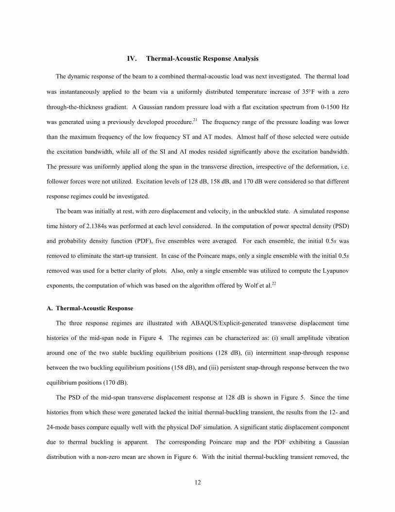
The three response regimes are illustrated with ABAQUS/Explicit-generated transverse displacement time

histories of the mid-span node in Figure 4. The regimes can be characterized as: (i) small amplitude vibration

around one of the two stable buckling equilibrium positions (128 dB), (ii) intermittent snap-through response

between the two buckling equilibrium positions (158 dB), and (iii) persistent snap-through response between the two

equilibrium positions (170 dB).

The PSD of the mid-span transverse displacement response at 128 dB is shown in Figure 5. Since the time

histories from which these were generated lacked the initial thermal-buckling transient, the results from the 12- and

24-mode bases compare equally well with the physical DoF simulation. A significant static displacement component

due to thermal buckling is apparent. The corresponding Poincare map and the PDF exhibiting a Gaussian

distribution with a non-zero mean are shown in Figure 6. With the initial thermal-buckling transient removed, the

12

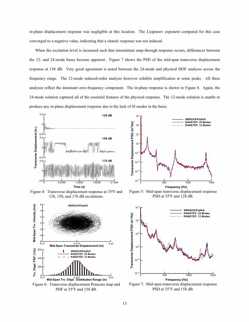
in-plane displacement response was negligible at this location. The Lyapunov exponent computed for this case

converged to a negative value, indicating that a chaotic response was not induced.

When the excitation level is increased such that intermittent snap-through response occurs, differences between

the 12- and 24-mode bases become apparent. Figure 7 shows the PSD of the mid-span transverse displacement

response at 158 dB. Very good agreement is noted between the 24-mode and physical DOF analyses across the

frequency range. The 12-mode reduced-order analysis however exhibits amplification at some peaks. All three

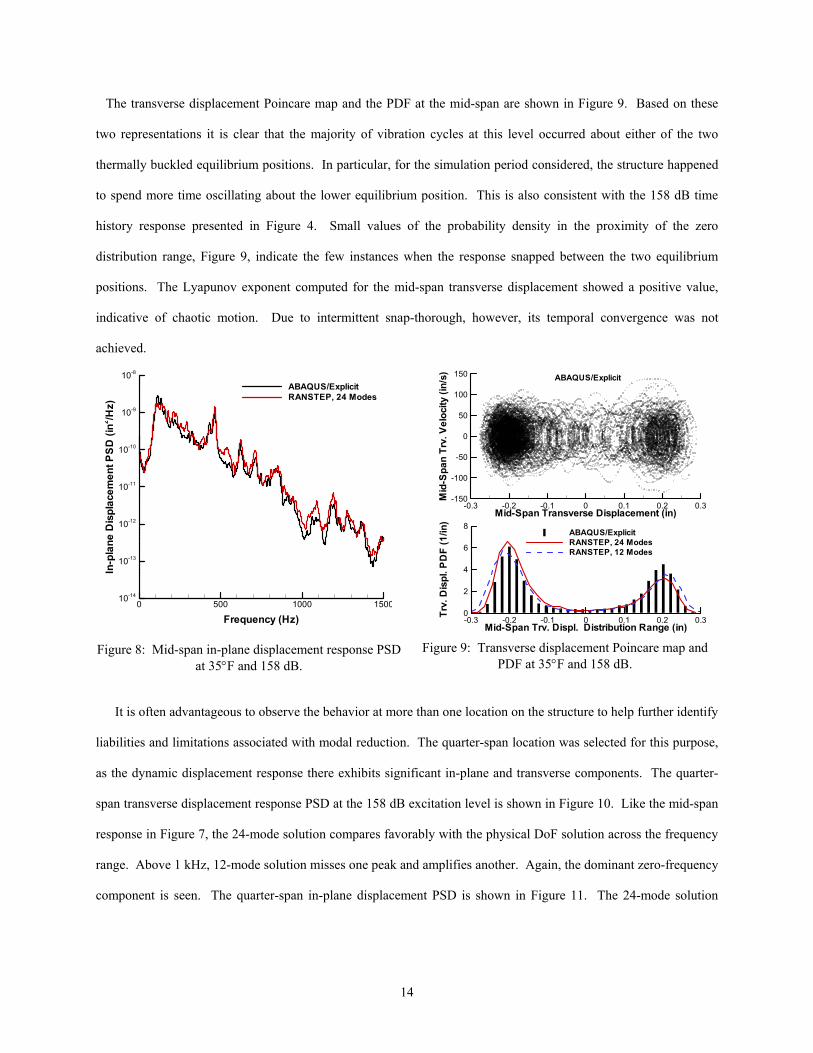
analyses reflect the dominant zero-frequency component. The in-plane response is shown in Figure 8. Again, the

24-mode solution captured all of the essential features of the physical response. The 12-mode solution is unable to

produce any in-plane displacement response due to the lack of SI modes in the basis.

-0.5

0

0.5

Time (s)0 0.5346 1.0692 1.6038 2.1384

-0.5

0

0.5

Tran

sver

seD

ispl

acem

ent(

in.)

-0.5

0

0.5

170 dB

128 dB

158 dB

Figure 4: Transverse displacement response at 35ºF and

128, 158, and 170 dB excitations.

Frequency (Hz)

Tran

sver

seD

ispl

acem

entP

SD

(in2 /H

z)

0 500 1000 150010-16

10-14

10-12

10-10

10-8

10-6

10-4

10-2

ABAQUS/ExplicitRANSTEP, 24 ModesRANSTEP, 12 Modes

Figure 5: Mid-span transverse displacement response

PSD at 35ºF and 128 dB.

Mid-Span Trv. Displ. Distribution Range (in)

Trv.

Dis

pl.P

DF

(1/in

)

0.21 0.215 0.220

200

400

600 ABAQUS/ExplicitRANSTEP, 24 ModesRANSTEP, 12 Modes

Mid-Span Transverse Displacement (in)

Mid

-Spa

nTr

v.V

eloc

ity(in

/s)

0.21 0.215 0.22-6

-4

-2

0

2

4

6 ABAQUS/Explicit

Figure 6: Transverse displacement Poincare map and

PDF at 35°F and 158 dB.

Frequency (Hz)

Tran

sver

seD

ispl

acem

entP

SD

(in2 /H

z)

0 500 1000 150010-12

10-10

10-8

10-6

10-4

10-2

ABAQUS/ExplicitRANSTEP, 24 ModesRANSTEP, 12 Modes

Figure 7: Mid-span transverse displacement response

PSD at 35°F and 158 dB.

13

The transverse displacement Poincare map and the PDF at the mid-span are shown in Figure 9. Based on these

two representations it is clear that the majority of vibration cycles at this level occurred about either of the two

thermally buckled equilibrium positions. In particular, for the simulation period considered, the structure happened

to spend more time oscillating about the lower equilibrium position. This is also consistent with the 158 dB time

history response presented in Figure 4. Small values of the probability density in the proximity of the zero

distribution range, Figure 9, indicate the few instances when the response snapped between the two equilibrium

positions. The Lyapunov exponent computed for the mid-span transverse displacement showed a positive value,

indicative of chaotic motion. Due to intermittent snap-thorough, however, its temporal convergence was not

achieved.

Frequency (Hz)

In-p

lane

Dis

plac

emen

tPS

D(in

2 /Hz)

0 500 1000 150010-14

10-13

10-12

10-11

10-10

10-9

10-8

ABAQUS/ExplicitRANSTEP, 24 Modes

Figure 8: Mid-span in-plane displacement response PSD at 35°F and 158 dB.

Mid-Span Transverse Displacement (in)

Mid

-Spa

nTr

v.V

eloc

ity(in

/s)

-0.3 -0.2 -0.1 0 0.1 0.2 0.3-150

-100

-50

0

50

100

150 ABAQUS/Explicit

Mid-Span Trv. Displ. Distribution Range (in)

Trv.

Dis

pl.P

DF

(1/in

)

-0.3 -0.2 -0.1 0 0.1 0.2 0.30

2

4

6

8ABAQUS/ExplicitRANSTEP, 24 ModesRANSTEP, 12 Modes

Figure 9: Transverse displacement Poincare map and PDF at 35°F and 158 dB.

It is often advantageous to observe the behavior at more than one location on the structure to help further identify

liabilities and limitations associated with modal reduction. The quarter-span location was selected for this purpose,

as the dynamic displacement response there exhibits significant in-plane and transverse components. The quarter-

span transverse displacement response PSD at the 158 dB excitation level is shown in Figure 10. Like the mid-span

response in Figure 7, the 24-mode solution compares favorably with the physical DoF solution across the frequency

range. Above 1 kHz, 12-mode solution misses one peak and amplifies another. Again, the dominant zero-frequency

component is seen. The quarter-span in-plane displacement PSD is shown in Figure 11. The 24-mode solution

14

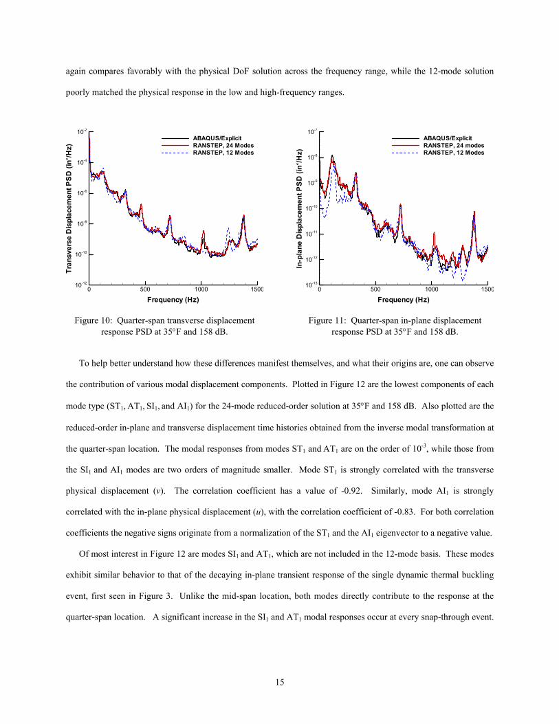
again compares favorably with the physical DoF solution across the frequency range, while the 12-mode solution

poorly matched the physical response in the low and high-frequency ranges.

Frequency (Hz)

Tran

sver

seD

ispl

acem

entP

SD

(in2 /H

z)

0 500 1000 150010-12

10-10

10-8

10-6

10-4

10-2

ABAQUS/ExplicitRANSTEP, 24 ModesRANSTEP, 12 Modes

Figure 10: Quarter-span transverse displacement response PSD at 35°F and 158 dB.

Frequency (Hz)In

-pla

neD

ispl

acem

entP

SD

(in2 /H

z)0 500 1000 1500

10-13

10-12

10-11

10-10

10-9

10-8

10-7

ABAQUS/ExplicitRANSTEP, 24 modesRANSTEP, 12 Modes

Figure 11: Quarter-span in-plane displacement response PSD at 35°F and 158 dB.

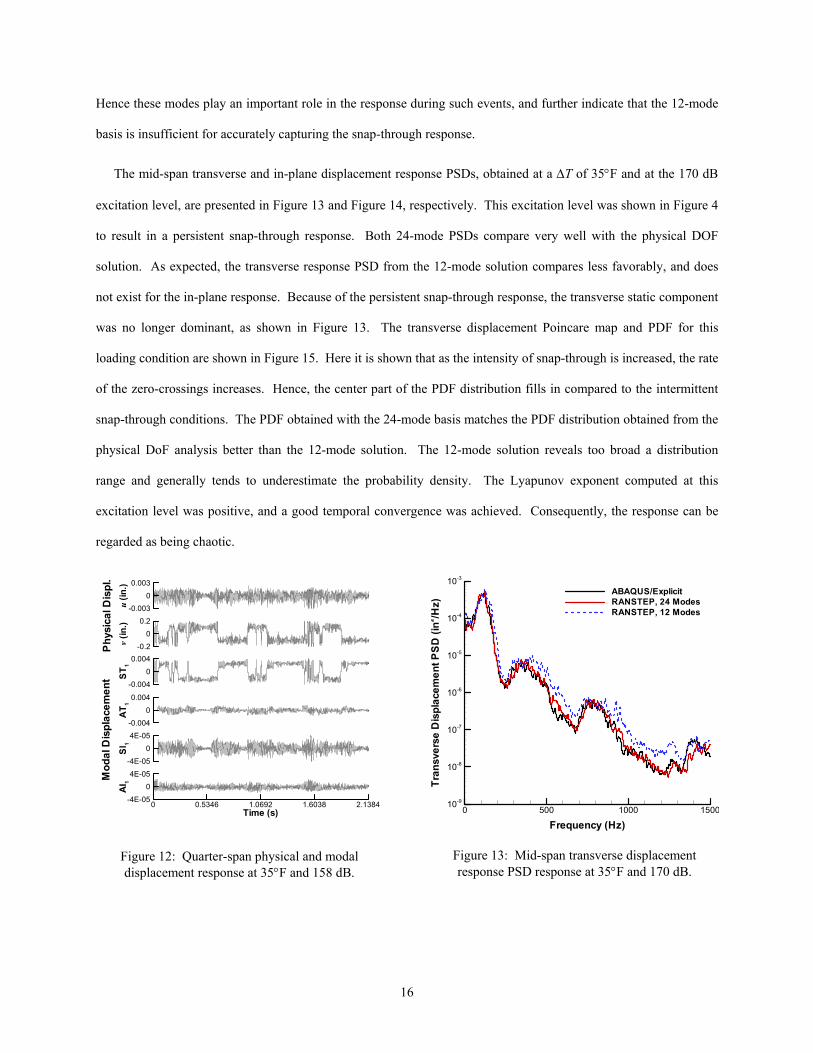
To help better understand how these differences manifest themselves, and what their origins are, one can observe

the contribution of various modal displacement components. Plotted in Figure 12 are the lowest components of each

mode type (ST1, AT1, SI1, and AI1) for the 24-mode reduced-order solution at 35°F and 158 dB. Also plotted are the

reduced-order in-plane and transverse displacement time histories obtained from the inverse modal transformation at

the quarter-span location. The modal responses from modes ST1 and AT1 are on the order of 10-3, while those from

the SI1 and AI1 modes are two orders of magnitude smaller. Mode ST1 is strongly correlated with the transverse

physical displacement (v). The correlation coefficient has a value of -0.92. Similarly, mode AI1 is strongly

correlated with the in-plane physical displacement (u), with the correlation coefficient of -0.83. For both correlation

coefficients the negative signs originate from a normalization of the ST1 and the AI1 eigenvector to a negative value.

Of most interest in Figure 12 are modes SI1 and AT1, which are not included in the 12-mode basis. These modes

exhibit similar behavior to that of the decaying in-plane transient response of the single dynamic thermal buckling

event, first seen in Figure 3. Unlike the mid-span location, both modes directly contribute to the response at the

quarter-span location. A significant increase in the SI1 and AT1 modal responses occur at every snap-through event.

15

Hence these modes play an important role in the response during such events, and further indicate that the 12-mode

basis is insufficient for accurately capturing the snap-through response.

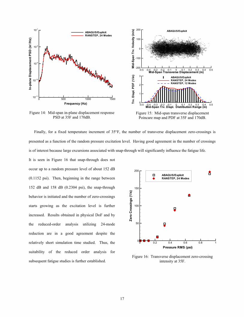
The mid-span transverse and in-plane displacement response PSDs, obtained at a ∆T of 35°F and at the 170 dB

excitation level, are presented in Figure 13 and Figure 14, respectively. This excitation level was shown in Figure 4

to result in a persistent snap-through response. Both 24-mode PSDs compare very well with the physical DOF

solution. As expected, the transverse response PSD from the 12-mode solution compares less favorably, and does

not exist for the in-plane response. Because of the persistent snap-through response, the transverse static component

was no longer dominant, as shown in Figure 13. The transverse displacement Poincare map and PDF for this

loading condition are shown in Figure 15. Here it is shown that as the intensity of snap-through is increased, the rate

of the zero-crossings increases. Hence, the center part of the PDF distribution fills in compared to the intermittent

snap-through conditions. The PDF obtained with the 24-mode basis matches the PDF distribution obtained from the

physical DoF analysis better than the 12-mode solution. The 12-mode solution reveals too broad a distribution

range and generally tends to underestimate the probability density. The Lyapunov exponent computed at this

excitation level was positive, and a good temporal convergence was achieved. Consequently, the response can be

regarded as being chaotic.

v(in

.)

-0.2

0

0.2

ST 1

-0.004

0

0.004

Phy

sica

lDis

pl.

Mod

alD

ispl

acem

ent

AT 1

-0.004

0

0.004

SI 1

-4E-05

0

4E-05

Time (s)

AI 1

0 0.5346 1.0692 1.6038 2.1384-4E-05

04E-05

u(in

.)

-0.0030

0.003

Figure 12: Quarter-span physical and modal displacement response at 35°F and 158 dB.

Frequency (Hz)

Tran

sver

seD

ispl

acem

entP

SD

(in2 /H

z)

0 500 1000 150010-9

10-8

10-7

10-6

10-5

10-4

10-3

ABAQUS/ExplicitRANSTEP, 24 ModesRANSTEP, 12 Modes

Figure 13: Mid-span transverse displacement response PSD response at 35°F and 170 dB.

16

Frequency (Hz)

In-p

lane

Dis

plac

emen

tPS

D(in

2 /Hz)

0 500 1000 150010-11

10-10

10-9

10-8

10-7

ABAQUS/ExplicitRANSTEP, 24 Modes

Figure 14: Mid-span in-plane displacement response PSD at 35F and 170dB.

Mid-Span Transverse Displacement (in)

Mid

-Spa

nTr

v.V

eloc

ity(in

/s)

-0.5 -0.4 -0.3 -0.2 -0.1 0 0.1 0.2 0.3 0.4 0.5-200

-100

0

100

200 ABAQUS/Explicit

Mid-Span Trv. Displ. Distribution Range (in)

Trv.

Dis

pl.P

DF

(1/in

)

-0.5 -0.4 -0.3 -0.2 -0.1 0 0.1 0.2 0.3 0.4 0.50

1

2

3 ABAQUS/ExplicitRANSTEP, 24 ModesRANSTEP, 12 Modes

Figure 15: Mid-span transverse displacement Poincare map and PDF at 35F and 170dB.

Finally, for a fixed temperature increment of 35°F, the number of transverse displacement zero-crossings is

presented as a function of the random pressure excitation level. Having good agreement in the number of crossings

is of interest because large excursions associated with snap-through will significantly influence the fatigue life.

It is seen in Figure 16 that snap-through does not

occur up to a random pressure level of about 152 dB

(0.1152 psi). Then, beginning in the range between

152 dB and 158 dB (0.2304 psi), the snap-through

behavior is initiated and the number of zero-crossings

starts growing as the excitation level is further

increased. Results obtained in physical DoF and by

the reduced-order analysis utilizing 24-mode

reduction are in a good agreement despite the

relatively short simulation time studied. Thus, the

suitability of the reduced order analysis for

subsequent fatigue studies is further established.

Pressure RMS (psi)

Zero

Cro

ssin

gs(1

/s)

0 0.2 0.4 0.6 0.80

50

100

150

200

1

ABAQUS/ExplicitRANSTEP, 24 Modes

Figure 16: Transverse displacement zero-crossing intensity at 35F.

17

V. Conclusion

A reduced-order FE based method for predicting thermo-acoustic random response in a nonlinear regime was

presented. Two sets of modal bases were examined in the study, and the corresponding reduced-order analysis

results were compared with solutions obtained with an analysis in physical DoF.

The effect of elevated temperature on the modal stiffness coefficients was first examined. It was found that only

the linear stiffness coefficients corresponding to low-frequency transverse displacement modes were affected by the

temperature change. These stiffness coefficients were found to vary linearly with temperature. Quadratic and cubic

stiffness coefficients were unaffected. As a result, a computational benefit may be gained for problems with a time-

varying thermal loading magnitude because linear coefficients need only be scaled.

In the analysis of dynamic thermal buckling and thermal-acoustic response, it was found that a modal basis

consisting of four types of modes (ST, AT, SI and AI) more accurately predicted the response than a basis consisting

of only ST and AI modes. In particular, for both loading conditions, the contribution of SI and AT modes becomes

more significant as the structure transitions to a different equilibrium position.

Although not in scope of this study, the fatigue life will be affected in a different manner depending on the

response regime. For the response about one of the thermally buckled equilibrium positions, a significant mean

stress component will be introduced. The mean stress has been shown to adversely affect the fatigue life.23,24

Additionally, for intermittent and persistent snap-through, large cyclic stress amplitudes will rapidly accumulate and

lead to a shorter fatigue life. Therefore, a continuation of this study to address stress recovery and fatigue estimation

is deemed to be worthwhile.

References

1Pozefsky, P., Blevins, R.D., and Langanelli, A.L., "Thermal-vibro-acoustic loads and fatigue of hypersonic flight vehicle

structure," Wright Labs, Wright Patterson Air Force Base AFWAL-TR-89-3014, 1989.

2Istenes, R.R., Rizzi, S.A., and Wolfe, H.F., "Experimental nonlinear random vibration results of thermally buckled composite

panels," Proceedings of the 36th AIAA/ASME/ASCE/AHS/ASC Structures, Structural Dynamics and Materials

Conference, AIAA-95-1345-CP, New Orleans, LA, 1995, pp. 1559-1568.

3Murphy, K.D., Virgin, L.N., and Rizzi, S.A., "Experimental snap-through boundaries for acoustically excited, thermally buckled

plates," Experimental Mechanics, Vol. 36, No. 4, 1996, pp. 312-317.

4Ng, C.F. and Clevenson, S.A., "High-intensity acoustic tests of a thermally stressed plate," Journal of Aircraft, Vol. 28, No. 4,

1991, pp. 275-281.

18

5Lee, J., "Displacement and strain histograms of thermally buckled composite plates in random vibration," Proceedings of the

37th AIAA/ASME/ASCE/AHS/ASC Structures, Structural Dynamics, and Materials Conference, AIAA-96-1347, Salt

Lake City, UT, 1996.

6Lee, J., "Displacement and strain statistics of thermally buckled plates," Journal of Aircraft, Vol. 38, No. 1, 2001, pp. 104-110.

7Lee, J., Vaicaitis, R., Wentz, K., Clay, C., Anselmo, E., and Crumbacher, R., "Predicition of statistical dynamics of thermally

buckled composite plates," Proceedings of the 39th AIAA/ASME/ASCE/AHS/ASC Structures, Structural Dynamics, and

Materials Conference, AIAA-98-1975, Long Beach, CA, 1998.

8Ng, C.F., "Nonlinear and snap-through response of curved panels to intense acoustic excitation," Journal of Aircraft, Vol. 26,

No. 3, 1989, pp. 281-288.

9Ng, C.F. and Wentz, K.R., "The prediction and measurement of thermoelastic response of plate structures," Proceedings of the

31st AIAA/ASME/ASCE/AHS/ASC Structures, Structural Dynamics, and Materials Conferece, AIAA-1990-988, Long

Beach, CA, 1990.

10Ghazarian, N. and Locke, J., "Nonlinear random response of antisymmetric angle-ply laminates under thermal-acoustic

loading," Journal of Sound and Vibration, Vol. 186, No. 2, 1995, pp. 291-309.

11Maekawa, S., "On the sonic fatigue life estimation of skin structures at room and elevated temperatures," Journal of Sound and

Vibration, Vol. 80, No. 1, 1982, pp. 41-59.

12Duan, B., Mei, C., and Ro, J.J., "Nonlinear response of thermal protection system at supersonic speeds," Proceedings of the

42nd AIAA/ASME/ASCE/AHS/ASC Structures, Structural Dynamics, and Materials Conference, AIAA-2001-1659,

Seattle, WA, 2001.

13Guo, X., Przekop, A., and Mei, C., "Nonlinear random response of shallow shells at elevated temperatures using finite element

modal method," Proceedings of the 45the AIAA/ASME/ASCE/AHS/ASC Structures, Structural Dynamics and Materials

Conference, AIAA-2004-1558, Palm Springs, CA, 2004.

14Mei, C., Dhainaut, J.M., Duan, B., Spottswood, S.M., and Wolfe, H.F., "Nonlinear random response of composite panels in an

elevated thermal environment," Air Force Research Laboratory AFRL-VA-WP-TR-2000-3049, Wright-Patterson Air

Force Base, OH, October 2000.

15Mignolet, M.P., Radu, A.G., and Gao, X., "Validation of reduced order modeling for the prediction of the response and fatigue

life of panels subjected to thermo-acoustic effects," Structural Dynamics: Recent Advances, Proceedings of the 8th

International Conference, The Institute of Sound and Vibration Research, University of Southampton, Southampton,

UK, 2003, M.J. Brennan, M.A. Ferman, B.A.T. Petersson, S.A. Rizzi, and K. Wentz (ed.).

16Muravyov, A.A. and Rizzi, S.A., "Determination of nonlinear stiffness with application to random vibration of geometrically

nonlinear structures," Computers and Structures, Vol. 81, No. 15, 2003, pp. 1513-1523.

19

17Rizzi, S.A. and Przekop, A., "The effect of basis selection on static and random acoustic response using a nonlinear modal

simulation," NASA Langley Research Center NASA/TP-2005-213943, Hampton, VA December 2005.

18Przekop, A. and Rizzi, S.A., "Nonlinear reduced order finite element analysis of structures with shallow curvature," AIAA

Journal, in press, 2006.

19Feeny, B.F., "On proper orthogonal co-ordinates as indicators of modal activity," Journal of Sound and Vibration, Vol. 255,

No. 5, 2002, pp. 805-817.

20Feeny, B.F. and Kappagantu, R., "On the physical interpretation of proper orthogonal modes in vibrations " Journal of Sound

and Vibration, Vol. 211, No. 4, 1998, pp. 607-616.

21Rizzi, S.A. and Muravyov, A.A., "Comparison of nonlinear random response using equivalent linearization and numerical

simulation," Structural Dynamics: Recent Advances, Proceedings of the 7th International Conference, Vol. 2, The

Institute of Sound and Vibration Research, University of Southampton, Southampton, UK, 2000, N.S. Ferguson, H.F.

Wolfe, M.A. Ferman, and S.A. Rizzi (ed.), pp. 833-846.

22Wolf, A., Swift, J.B., Swinney, H.L., and Vastano, J.A., "Determining Lyapunov exponents from a time series," Physica, Vol.

16D, No. 1985, pp. 285-317.

23Rizzi, S.A. and Przekop, A., "Estimation of sonic fatigue by reduced-order finite element based analysis," Structural Dynamics:

Recent Advances, Proceedings of the 9th International Conference, The Institute of Sound and Vibration Research,

University of Southampton, Southampton, UK, 2006, M.J. Brennan, B.R. Mace, J.M. Muggleton, B.A.T. Petersson,

K.D. Murphy, S.A. Rizzi, and R. Shen (ed.).

24Sweitzer, K.A. and Ferguson, N.S., "Mean stress effects on random fatigue of nonlinear structures," Proceedings of the XII

International Congress on Sound and Vibration, Lisbon, Portugal, 2005.

20