PHYSICAL REVIEW A 87, 023835 (2013)

Dynamical correlation functions and the quantum Rabi model

F. A. Wolf,1 F. Vallone,2 G. Romero,2 M. Kollar,3 E. Solano,2,4 and D. Braak1

1Experimental Physics VI, Center for Electronic Correlations and Magnetism, University of Augsburg, 86135 Augsburg, Germany2Departamento de Quımica Fısica, Universidad del Paıs Vasco UPV/EHU, Apartado 644, 48080 Bilbao, Spain

3Theoretical Physics III, Center for Electronic Correlations and Magnetism, University of Augsburg, 86135 Augsburg, Germany4IKERBASQUE, Basque Foundation for Science, Alameda Urquijo 36, 48011 Bilbao, Spain

(Received 7 December 2012; published 22 February 2013)

We study the quantum Rabi model within the framework of the analytical solution developed in Phys. Rev. Lett.107, 100401 (2011). In particular, through time-dependent correlation functions, we give a quantitative criterionfor classifying two regions of the quantum Rabi model, involving the Jaynes-Cummings, the ultrastrong-coupling,and the deep strong-coupling regimes. In addition, we find a stationary qubit-field entangled basis that governsthe whole dynamics as the coupling strength overcomes the mode frequency.

DOI: 10.1103/PhysRevA.87.023835 PACS number(s): 42.50.Pq, 03.65.Ge, 02.30.Ik

I. INTRODUCTION

The light-matter interaction has been a subject of centralinterest since the early years of quantum mechanics. In1936, one of the first attempts to explain the results comingfrom experiments was the Rabi model, which describes thesimplest dipole semiclassical interaction between light andmatter [1], and is reduced to a pseudospin-1/2 system drivenby a monochromatic classical radiation field. However, theadvent of quantum technologies such as cavity QED [2,3] hasallowed us to access the quantum regime of the radiation field,where the dynamical description is given by the celebratedJaynes-Cummings model (JCM) [4]. This model predictscollapses and revivals of the population inversion and theappearance of Jaynes-Cummings doublets as a consequenceof the excitation-number conservation, and it has found atest bed in several hybrid setups such as trapped ions [5],quantum dots [6], and circuit quantum electrodynamics (circuitQED) [7–16].

The field of circuit QED has been growing both the-oretically and experimentally, and complex proposals suchas the generation of multipartite entanglement [17–19] relyon the fundamentals of the JCM and the Tavis-Cummingsmodel [20]. This can be justified because the ratio betweenthe coupling strength g and the resonator frequency ω maygrow from typical quantum optical values of g/ω ∼ 10−6 tocircuit QED values of g/ω ∼ 10−2. Note that, in the lattercase, the rotating-wave approximation (RWA) can still be ap-plied. Nowadays, two key experiments with superconductingcircuits [21,22] have made a significant improvement in thecoupling strength, reaching values g/ω ∼ 0.1 in the so-calledultrastrong-coupling (USC) regime [23–25]. In this case, theRWA is not longer valid and all dynamical and static propertieshave to be explained through the quantum Rabi model (QRM)

HR = h�σz + hωa†a + hgσx(a + a†), (1)

where σz and σx are Pauli matrices, a (a†) is the annihilation(creation) operator, � ≡ ωq/2 is half of the qubit energy, ω isthe resonator frequency, and g stands for the coupling strength.In addition, a recent proposal considers the case where thecoupling strength g becomes comparable to or larger thanthe mode frequency ω, g/ω � 1, which is called the deepstrong-coupling (DSC) regime [26]. In this case, the dynamics

can be intuitively explained as photon-number wave packetspropagating along a defined parity chain. Although the state ofthe art in circuit QED does not provide this coupling strengthyet, the main features of the DSC regime have been observedin an analog quantum simulation [27,28].

The QRM described by the Hamiltonian (1) has substantialdifferences as compared to the JCM; in fact only recentlyhave the properties of the QRM been completely understood[29,30]. In the QRM, a discrete Z2 symmetry replacesthe continuous U(1) symmetry of the JCM. Therefore theexcitation number is no longer a conserved quantity and theHilbert space splits into two infinite-dimensional invariantsubspaces, the parity chains [26]. Each eigenstate can belabeled with a Z2 quantum number, the parity P = σze

iπa†a

taking values ±1.Furthermore, it is possible to give analytical expressions

for these eigenstates as elements of the Bargmann space [31],which allows the well-defined computation of their norms andoverlaps with eigenstates of the harmonic oscillator, withouttruncation of the Hilbert space [32].

The aim of this work is to present additional insight intothe quantum Rabi model by stressing the use of dynamicalcorrelation functions coming from the analytical solutionobtained in Ref. [29]. In this manner, we are able to explainrelevant features such as the validity of the RWA in twowell-defined regions, ranging from the JC regime to higher-coupling regimes of the quantum Rabi model. In addition, asthe coupling strength g enters into the DSC regime, we find thatthe true eigenstates of the system can be well approximatedby the shifted oscillator basis in each invariant parity chainwithout the need for a more complicated basis. This fact issupported by the calculation of the Wigner function of theeigenstates, whose unexpected fidelity can be understood interms of the analytical form of the eigenfunctions [29], closelyresembling Fock states. In this context, we also find stationarySchrodinger-cat-like states in the DSC regime. Finally, wepresent our concluding remarks.

II. DYNAMICAL CLASSIFICATION

In this section, we shall use the exact dynamics of thequantum Rabi model to characterize two coupling regions that

023835-11050-2947/2013/87(2)/023835(7) ©2013 American Physical Society

WOLF, VALLONE, ROMERO, KOLLAR, SOLANO, AND BRAAK PHYSICAL REVIEW A 87, 023835 (2013)

we may call the lower-coupling region and the higher-couplingregion, respectively. The first region comprises the JC regime,where the RWA holds, together with the perturbative USCregime, where small deviations from the JCM occur (g/ω �0.1). The second identified region comprises a jump towardsthe higher-coupling regime, g/ω � 0.4, and forms a precursorof the DSC regime (g/ω > 1). The intermediate region, thatis, for 0.1/ω � g/ω � 0.4, determines a kind of dark zonewhere no intuitive physics has been identified up to now.

We begin by studying a suitable dynamical observable, thetime-averaged photon number

n0 = limt→∞

1

t

∫ t

0dt ′n0(t ′), (2)

which measures the breaking of the U(1) symmetry in the JCM.As we will show, this quantity exhibits significant features thatcharacterize the regions mentioned before.

Since HR commutes with the parity operator P , it is usefulto investigate the dynamics within a fixed-parity chain. Let |σ 〉with σ = ±1 correspond to the states |e〉 and |g〉 of the two-level system, respectively. Then the subspace H± with parity±1 is spanned by states {|φs〉 ⊗ |±σ 〉,|φa〉 ⊗ |∓σ 〉} where|φ(a),s〉 denotes the (anti)symmetric part of |φ〉, which is anelement of the Hilbert space Hb of the radiation mode. Hb isspanned by Fock states {|n〉}, which are (anti)symmetric if n

is (odd) even.There exists a transformation F± that maps the element |φ〉

of Hb onto a parity eigenstate |φ,±〉 that belongs to a paritychain

F±|φ〉 = |φ,±〉 = φs ⊗ |±σ 〉 + φa ⊗ |∓σ 〉. (3)

The dynamical quantities in each chain depend only on theinitial distribution of photons, which fixes |φ(t),±〉 at timet = 0. The state at later times follows as the solution of theSchrodinger equation

i∂t |φ(t)〉 = H±|φ(t)〉, (4)

where H± acts on functions in Hb [32]. The natural observablewithin the invariant subspaces is thus the photon number.

We consider first the time-dependent expectation valuenφ(t) = 〈φ(t),+|a†a|φ(t),+〉 for some initial |φ(0)〉 andpositive parity. For � = 0 and an initial Fock state |φ(0)〉 =|m〉 = (a†)m/

√m!|0〉, the average photon number at time t

reads (g = g/ω)

nm(t) = m + 2g2[1 − cos(ωt)], (5)

which entails that the difference nm(t) − m is independentof the initial photon number, always greater than zero, andoscillates with the mode frequency ω. Because Fock stateshave definite reflection symmetry, the initial state in the fullHilbert space will be the product |m〉 ⊗ |(−1)m〉 ∈ H+.

Starting now from the photon vacuum |0〉 we considervalues � = 0. Then the correlation function n0(t) depends onthe initial state and shows a complicated oscillatory behavior.Still the time evolution can be globally characterized by thetime-averaged quantity defined in Eq. (2). Its dependence on� ≡ �/ω for fixed g shows features that allow a regime whichcorresponds to the validity of the RWA (the JC regime) to bedistinguished from a region where the nonconservation of theexcitation number in the QRM becomes relevant. As shown

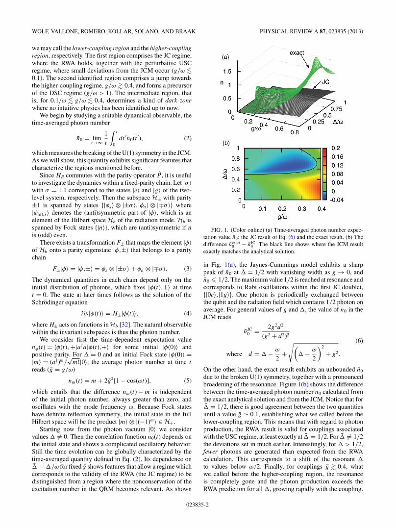
FIG. 1. (Color online) (a) Time-averaged photon number expec-tation value n0: the JC result of Eq. (6) and the exact result. (b) Thedifference nexact

0 − nJC0 . The black line shows where the JCM result

exactly matches the analytical solution.

in Fig. 1(a), the Jaynes-Cummings model exhibits a sharppeak of n0 at � = 1/2 with vanishing width as g → 0, andn0 � 1/2. The maximum value 1/2 is reached at resonance andcorresponds to Rabi oscillations within the first JC doublet,{|0e〉,|1g〉}. One photon is periodically exchanged betweenthe qubit and the radiation field which contains 1/2 photon onaverage. For general values of g and �, the value of n0 in theJCM reads

nJC0 = 2g2d2

(g2 + d2)2

(6)

where d = � − ω

2+

√(� − ω

2

)2

+ g2.

On the other hand, the exact result exhibits an unbounded n0

due to the broken U(1) symmetry, together with a pronouncedbroadening of the resonance. Figure 1(b) shows the differencebetween the time-averaged photon number n0 calculated fromthe exact analytical solution and from the JCM. Notice that for� = 1/2, there is good agreement between the two quantitiesuntil a value g ∼ 0.1, establishing what we called before thelower-coupling region. This means that with regard to photonproduction, the RWA result is valid for couplings associatedwith the USC regime, at least exactly at � = 1/2. For � = 1/2the deviations set in much earlier. Interestingly, for � > 1/2,fewer photons are generated than expected from the RWAcalculation. This corresponds to a shift of the resonant �

to values below ω/2. Finally, for couplings g � 0.4, whatwe called before the higher-coupling region, the resonanceis completely gone and the photon production exceeds theRWA prediction for all �, growing rapidly with the coupling.

023835-2

DYNAMICAL CORRELATION FUNCTIONS AND THE . . . PHYSICAL REVIEW A 87, 023835 (2013)

0

0.2

0.4

0.6

0.8

1P

0(a)

g=0.1 g=0.7 g=2.0

0

0.2

0.4

0.6

0.8

1

0 1 2 3 4 5

P4

tω/(2π)

(b)

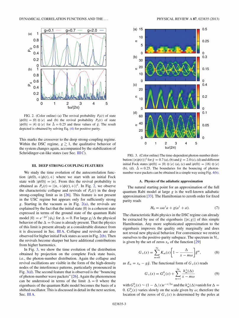
FIG. 2. (Color online) (a) The revival probability P0(t) of state|φ(0)〉 = |0〉 ⊗ |e〉 and (b) the revival probability P4(t) of state|φ(0)〉 = |4〉 ⊗ |e〉 for � = 0.25 and three values of g. The resultdepicted is obtained by solving Eq. (4) for positive parity.

This marks the crossover to the deep strong-coupling regime.Within the DSC regime, g � 1, the qualitative behavior ofthe system changes again, accompanied by the stabilization ofSchrodinger-cat-like states (see Sec. III C).

III. DEEP STRONG-COUPLING FEATURES

We study the time evolution of the autocorrelation func-tion 〈φ(0),+|φ(t),+〉 where we start with an initial Fockstate with |φ(0)〉 = |n〉. From this the revival probability isobtained as Pn(t) = |〈n,+|φ(t),+〉|2. In Fig. 2, we observethe characteristic collapse and revivals of Pn(t) in the deepstrong-coupling limit as in [26]. This feature is not presentin the USC regime but appears only for sufficiently strongg. Starting in the vacuum as in Fig. 2(a), the revivals areexplained by the fact that the initial state |0〉 is a coherent stateexpressed in terms of the ground state of the quantum Rabimodel |0〉 = e−ga† |ψ0〉 for � = 0. For large g/� the physicalbehavior of the � = 0 case is already present. That the physicsof this limit is present already at a considerable distance fromit is discussed in Sec. III A. Collapse and revivals are alsoobserved for higher initial Fock states as seen in Fig. 2(b). Thenthe revivals become sharper but have additional contributionsfrom higher harmonics.

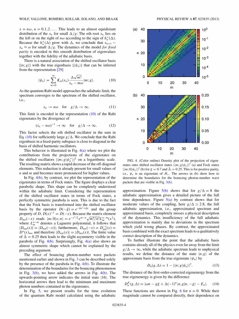
In Fig. 3, we show the time evolution of the distributionobtained by projection on the complete Fock state basis,i.e., the photon-number distribution. Again the collapse andrevival oscillations are visible in the form of the high-densitynodes of the interference patterns, particularly pronounced inFig. 3(d). The second feature that is observed is the “bouncingof photon-number wave packets” [26]. Again the phenomenoncan be understood in terms of the limit � = 0 where theeigenbasis of the quantum Rabi model becomes the basis of ashifted oscillator. This is discussed in detail in the next section,Sec. III A.

FIG. 3. (Color online) The time-dependent photon-number distri-bution |〈n|φ(t)〉|2 for g = 0.7 (a), (b) and g = 2.0 (c), (d) and differentinitial Fock states |φ(0)〉 = |0〉 ⊗ |e〉 (a), (c) and |φ(0)〉 = |16〉 ⊗ |e〉(b), (d). � = 0.25. The boundaries for the bouncing of photon-number wave packets can be obtained in a simple way using Fig. 4(b).

A. Physics of the adiabatic approximation

The natural starting point for an approximation of the fullquantum Rabi model at large g is the well-known adiabaticapproximation [33]. The Hamiltonian to zeroth order for fixedparity reads

H0 = ωa†a + g(a† + a). (7)

The characteristic Rabi physics in the DSC regime can alreadybe extracted by use of the eigenbasis {|n; g〉} of this simpleHamiltonian. Any more sophisticated approximation to theeigenbasis improves the quality only marginally and doesnot reveal new physical behavior. For convenience we restrictourselves to the positive-parity subspace. The spectrum in H+is given by the set of zeros xn of the function [29]

G+(x) =∞∑

m=0

Km(x)

[1 − �

x − mω

]gm, (8)

as En = xn − gg. The functional form of G+(x) reads

G+(x) = G0+(x) +

∞∑m=1

h+m(�)

x − mω(9)

with G0+(x) ∼ (1 − �/x)e−x/2ω and the h+

m(�) vanish for � =0. G0

+(x) varies slowly on the scale given by ω; therefore thelocation of the zeros of G+(x) is determined by the poles at

023835-3

WOLF, VALLONE, ROMERO, KOLLAR, SOLANO, AND BRAAK PHYSICAL REVIEW A 87, 023835 (2013)

x = nω, n = 0,1,2 . . . . This leads to an almost equidistantdistribution of the xn for small �/g: The nth root xn lies onthe left or on the right of nω according to the sign of h+

n (�).Because the h+

n (�) grow with �, we conclude that xn+1 −xn ≈ ω for small �/g. The dynamics of the model for fixedparity is encoded in this smooth distribution of eigenvaluestogether with the fidelity of the adiabatic basis.

There is a natural association of the shifted oscillator basis{|n; g〉} with the true eigenbasis {|ψn〉} that can be inferredfrom the representation [29]

|ψn〉 =∞∑

m=0

Km(xn)�

√m!

xn − mω|m; g〉. (10)

As the quantum Rabi model approaches the adiabatic limit, thespectrum converges to the spectrum of the shifted oscillator,i.e.,

xn → nω for g/� → ∞. (11)

This limit is encoded in the representation (10) of the Rabieigenstates by the divergence of

(xn − nω)−1 → ∞ for g/� → ∞. (12)

This factor selects the nth shifted oscillator in the sum inEq. (10) for sufficiently large g/�. We conclude that the Rabieigenbasis in a fixed-parity subspace is close to diagonal in thebasis of shifted harmonic oscillators.

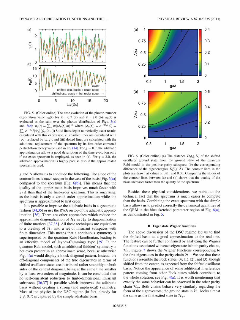
This behavior is illustrated in Fig. 4(a) where we plot thecontributions from the projections of the eigenstates onthe shifted oscillators |〈m; g|ψ+

n 〉|2 on a logarithmic scale.The resulting matrix shows a rapid decrease of the off-diagonalelements. This reduction is already present for small values ofn and m and becomes more pronounced for higher values.

In Fig. 4(b), by contrast, we plot the representation of theeigenstates in terms of Fock states. The figure displays a clearparabolic shape. This shape can be completely understoodwithin the adiabatic limit. Considering the representationof the shifted oscillator states in terms of Fock states, aperfectly symmetric parabola is seen. This is due to the factthat the Fock basis is transformed into the shifted oscillatorbasis by the operator D(−g) = e−ga†+ga and the groupproperty of D, D(x)−1 = D(−x). Because the matrix elementDmn(−x) reads 〈m; 0|x; n〉 = e−x2/2xm−n

√m!/n!Ln−m

m (x2),where Ln−m

m denotes a Laguerre polynomial, it follows that|Dnm(x)| = |Dnm(−x)|; furthermore, Dnm(−x) = D−1

nm(x) =D∗(x)mn and therefore |Dnm(x)| = |Dmn(x)|. The finite valueof � = 0.25 then leads to the slight asymmetry visible in theparabola of Fig. 4(b). Surprisingly, Fig. 4(a) also shows analmost symmetric shape which cannot be explained by thepreceding argument.

The effect of bouncing photon-number wave packetsmentioned earlier and shown in Fig. 3 can be described solelyby the presence of the parabola in Fig. 4(b). To illustrate thedetermination of the boundaries for the bouncing phenomenonin Fig. 3(b), we have added the arrows in Fig. 4(b). Theupwards-pointing arrow indicates the initial state |16〉. Thehorizontal arrows then lead to the minimum and maximumphoton numbers contained in the eigenstates.

In Fig. 5, we present results for the time evolutionof the quantum Rabi model calculated using the adiabatic

FIG. 4. (Color online) Density plot of the projection of eigen-states onto shifted oscillator states |〈m; g|ψn〉|2 (a) and Fock states|〈m; 0|ψn〉|2 (b) for g = 0.7 and � = 0.25. This is for positive parity,i.e., ψn is an eigenstate of H+. The arrows in (b) show how todetermine the boundaries for the bouncing photon-number wavepackets that are visible in Fig. 3(b).

approximation. Figure 5(b) shows that for g/� = 8 theadiabatic approximation gives a detailed picture of the fulltime dependence. Figure 5(a) by contrast shows that formoderate values of the coupling, here g/� � 2.8, the fulladiabatic approximation, i.e., approximated spectrum andapproximated basis, completely misses a physical descriptionof the dynamics. This insufficiency of the full adiabaticapproximation is mainly due to deviations in the spectrumwhich yield wrong phases. By contrast, the approximatedbasis combined with the exact spectrum leads to a qualitativelycorrect description of the dynamics.

To further illustrate the point that the adiabatic basiscontains already all of the physics even far away from the limitg/� → ∞, while the adiabatic spectrum leads to unphysicalresults, we define the distance of the state |n,g〉 of theapproximate basis from the true eigenstate |ψn〉 by

Dn(g,�) = 1 − |〈n; g|ψn〉|2. (13)

The distance of the first-order-corrected eigenenergy from thetrue eigenenergy is given by the difference

DEn (g,�) = |ωn − gg + �(−1)n〈n,g|n,−g〉 − En|. (14)

These functions are shown in Fig. 6 for n = 0. While theirmagnitude cannot be compared directly, their dependence on

023835-4

DYNAMICAL CORRELATION FUNCTIONS AND THE . . . PHYSICAL REVIEW A 87, 023835 (2013)

0

1

2

n 0(t

)(a)

0

5

10

15

0 5 10 15 20

n 0(t

)

tω/(2π)

(b)

exactshifted osc. basis + exact spec.

shifted osc. basis + first order spec.

FIG. 5. (Color online) The time evolution of the photon-numberexpectation value n0(t) for g = 0.7 (a) and g = 2.0 (b). n0(t) isevaluated as the sum over the photon distribution of Figs. 3(a)and 3(c): n0(t) = ∑

m m|〈φ0(t)|m〉|2 where |φ0(t)〉 = e−iH+t |0〉 =∑n e−iE+

n t |ψn〉〈ψn|0〉. (i) Solid lines depict numerically exact resultscalculated with this expression, (ii) dashed lines are calculated with|ψn〉 replaced by |n,g〉, and (iii) dotted lines are calculated with theadditional replacement of the spectrum by its first-order-correctedperturbation theory value used in Eq. (14). For g = 0.7, the adiabaticapproximation allows a good description of the time evolution onlyif the exact spectrum is employed, as seen in (a). For g = 2.0, theadiabatic approximation is highly precise also if the approximatedspectrum is used.

g and � allows us to conclude the following. The slope of thecontour lines is much steeper in the case of the basis [Fig. 6(a)]compared to the spectrum [Fig. 6(b)]. This means that thequality of the approximate basis improves much faster withg/� than that of the first-order spectrum. This is surprising,as the basis is only a zeroth-order approximation while thespectrum is approximated to first order.

It is possible to improve the adiabatic basis in a systematicfashion [34,35] or use the RWA on top of the adiabatic approx-imation [36]. There are other approaches which reduce theapproximate diagonalization of HR in H± to diagonalizationof finite matrices [37,38]. All these techniques are equivalentto a breakup of H± into a set of invariant subspaces withfinite dimension. This means that a continuous symmetry issuperimposed on the quantum Rabi Hamiltonian, leading toan effective model of Jaynes-Cummings type [29]. In thequantum Rabi model, such an additional (hidden) symmetry isnot even present in an approximate sense, because otherwiseFig. 4(a) would display a block-diagonal pattern. Instead, theoff-diagonal components of the true eigenstates in terms ofshifted oscillator states are distributed rather smoothly on bothsides of the central diagonal, being at the same time smallerby at least two orders of magnitude. It can be concluded thatno self-consistent reduction to finite-dimensional invariantsubspaces [36,37] is possible which improves the adiabaticbasis without creating a strong (and unphysical) symmetry.Most of the physics in the DSC regime (in fact, already forg � 0.7) is captured by the simple adiabatic basis.

FIG. 6. (Color online) (a) The distance D0(g,�) of the shiftedoscillator ground state from the ground state of the quantumRabi model in the positive-parity subspace; (b) the correspondingdifference of the eigenenergies DE

0 (g,�). The contour lines in theplots are drawn at values of 0.01 and 0.05. Comparing the slopes ofthe contour lines between (a) and (b) shows that the quality of thebasis increases faster than the quality of the spectrum.

Besides these physical considerations, we point out thetechnical fact that the spectrum is much easier to computethan the basis. Combining the exact spectrum with the simplebasis allows us to predict correctly the dynamical quantities ofthe QRM in the blue sketched parameter region of Fig. 6(a),as demonstrated in Fig. 5.

B. Eigenstate Wigner functions

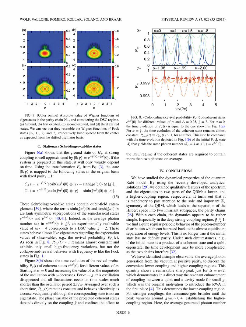
The above discussion of the DSC regime led us to findthe shifted basis as a good approximation to the real one.The feature can be further confirmed by analyzing the Wignerfunctions associated with each eigenstate in both parity chains,H±. Figure 7 shows the Wigner functions corresponding tothe first eigenstates in the parity chain H−. We see that thesefunctions resemble the Fock states |0〉, |1〉, |2〉, and |3〉, thoughshifted from the center, as expected from the shifted oscillatorbasis. Notice the appearance of some additional interferencepattern coming from other Fock states which contribute tothe whole solution; see Fig. 4(a). It is worth mentioning thatexactly the same behavior can be observed in the other paritychain H+. Both chains behave very similarly regarding theform of the eigenvectors; the ground state in H− looks almostthe same as the first exited state in H+.

023835-5

WOLF, VALLONE, ROMERO, KOLLAR, SOLANO, AND BRAAK PHYSICAL REVIEW A 87, 023835 (2013)

FIG. 7. (Color online) Absolute value of Wigner functions ofeigenstates in the parity chain H−, and considering the DSC regime.(a) Ground, (b) first excited, (c) second excited, and (d) third excitedstates. We can see that they resemble the Wigner functions of Fockstates |0〉, |1〉, |2〉, and |3〉, respectively, but displaced from the centeras expected from the shifted oscillator basis.

C. Stationary Schrodinger-cat-like states

Figure 6(a) shows that the ground state of H+ at strongcoupling is well approximated by |0; g〉 = e−g2/2−ga† |0〉. If thesystem is prepared in this state, it will only weakly dependon time. Using the transformation F± from Eq. (3), the state|0; g〉 is mapped to the following states in the original basiswith fixed parity ±1:

|C+〉 = e−g2/2[cosh(ga†)|0〉 ⊗ |e〉 − sinh(ga†)|0〉 ⊗ |g〉],|C−〉 = e−g2/2[cosh(ga†)|0〉 ⊗ |g〉 − sinh(ga†)|0〉 ⊗ |e〉].

(15)

These Schrodinger-cat-like states contain qubit-field entan-glement [39], where the terms sinh(ga†)|0〉 and cosh(ga†)|0〉are (anti)symmetric superpositions of the semiclassical statese−ga† |0〉 and ega† |0〉 [40,41]. Indeed, as the average photonnumber 〈n〉 in e±ga† |0〉 is g2, an experimentally realizablevalue of 〈n〉 = 4 corresponds to a DSC value g = 2. Thesestates behave almost like eigenstates regarding the expectationvalues of observables, e.g., the revival probability PC± (t).As seen in Fig. 8, PC±(t) ∼ 1 remains almost constant andexhibits only small high-frequency variations, but not thecollapse-and-revival behavior with frequency ω like the Fockstates in Fig. 1.

Figure 8(b) shows the time evolution of the revival proba-bility Pα(t) of coherent states eαa† |0〉 for different values of α.Starting at α = 0 and increasing the value of α, the magnitudeof the oscillation with ω decreases. For α = g, this oscillationdisappeared and all fluctuations occur on time scales muchshorter than the oscillator period 2π/ω. Averaged over such ashort time, PC±(t) remains constant and behaves effectively asa conserved quantity although the corresponding state is not aneigenstate. The phase variable of the protected coherent statesdepends directly on the coupling g and confines the effect to

0

0.2

0.4

0.6

0.8

1

Pα

(a) α=0 α=1 α=1.5 α=1.8

0.998

0.999

1

0 1 2 3 4 5

Pα

tω/(2π)

(b) α=1.98 α=1.99 α=2.00

FIG. 8. (Color online) Revival probability Pα(t) of coherent stateseαa† |0〉 for different values of α and � = 0.25, g = 2. For α = 0,the time evolution of Pα(t) is equal to the one shown in Fig. 1(a).For α = g, the time evolution of the coherent state remains almostconstant, Pα=g(t) ≡ PC+ (t) ∼ 1, for all times. This is to be comparedwith the time evolution depicted in Fig. 1(b) of the initial Fock state|4〉 that yields the same photon number 〈n〉 = 4 as |C+〉 = e2a† |0〉.

the DSC regime if the coherent states are required to containmore than two photons on average.

IV. CONCLUSIONS

We have studied the dynamical properties of the quantumRabi model. By using the recently developed analyticalsolutions [29], we obtained qualitative features of the spectrumand the eigenstates in two parts of the QRM: a lower- anda higher-coupling region, respectively. It turns out that itis mandatory to pay attention to the sole and important Z2

symmetry of the QRM, which leads to the separation of theHilbert space into two invariant subspaces, the parity chains[26]. Within each chain, the dynamics appears to be rathersimple. Especially in the deep strong-coupling regime, g � 1,we find a quite regular periodic behavior of the photon-numberdistribution which can be traced back to the almost equidistantseparation of energy levels. This is no longer true if the initialstate has no definite parity. Under such circumstances, e.g.,if the initial state is a product of a coherent state and a qubiteigenstate, the time development may be more complicated,as the two chains interfere [32].

We have identified a simple observable, the average photongeneration from the vacuum at positive parity, to discern theconvenient lower-coupling and higher-coupling regions. Thisquantity shows a remarkable sharp peak just for � = ω/2,which demonstrates in a direct way the resonant enhancementof coupling between a qubit and a cavity mode for small g,which was the original motivation to introduce the RWA inthe first place [4]. This determines the lower-coupling region.For stronger couplings, the resonance gets broader until thepeak vanishes around g/ω ∼ 0.4, establishing the higher-coupling region. Here, the average generated photon number

023835-6

DYNAMICAL CORRELATION FUNCTIONS AND THE . . . PHYSICAL REVIEW A 87, 023835 (2013)

becomes larger than the JC limit of 1/2 due to the counter-rotating terms in (1), which break the conservation law ofthe JCM.

As early as for g/ω � 0.7, the characteristic features ofthe deep strong-coupling regime begin to materialize. Thedynamics for fixed parity are dominated by the adiabaticbasis and the almost equidistant spectrum. Interestingly, thenontrivial effects which separate the QRM in this regime fromthe simple adiabatic limit can be incorporated by using theexact spectrum together with the adiabatic basis. In fact, theexact eigenstates are very close to their adiabatic approximantswhereas deviations in the eigenvalues lead to phase differenceswhich become apparent after longer times (Fig. 5). The fidelityof the adiabatic basis is even more visible in the Wignerrepresentation, which demonstrates the similarity of parity

eigenstates to Fock states in the deep strong-coupling regime(Fig. 7).

Finally, the DSC regime allows for a special class of stateswhich are not exact eigenstates but lead to expectation valuesfluctuating with small amplitudes on very short time scales.In this sense, they form stationary Schrodinger-cat-like states,unaffected by the system interaction.

ACKNOWLEDGMENTS

We acknowledge funding from the Deutsche Forschungs-gemeinschaft through TRR 80, the Spanish MINECOFIS2012-36673-C03-02; UPV/EHU UFI 11/55; Basque Gov-ernment IT472-10; SOLID, CCQED, PROMISCE, andSCALEQIT European projects.

[1] I. I. Rabi, Phys. Rev. 49, 324 (1936); 51, 652 (1937).[2] H. Walther, B. T. H. Varcoe, B.-G. Englert, and T. Becker, Rep.

Prog. Phys. 69, 1325 (2006).[3] S. Haroche and J.-M. Raymond, Exploring the Quantum (Oxford

University Press, New York, 2006).[4] E. T. Jaynes and F. W. Cummings, Proc. IEEE 51, 89

(1963).[5] D. Leibfried, R. Blatt, C. Monroe, and D. Wineland, Rev. Mod.

Phys. 75, 281 (2003).[6] R. Hanson, L. P. Kouwenhoven, J. R. Petta, S. Tarucha, and

L. M. K. Vandersypen, Rev. Mod. Phys. 79, 1217 (2007).[7] A. Wallraff, D. I. Schuster, A. Blais, L. Frunzio, R.-S. Huang,

J. Majer, S. Kumar, S. M. Girvin, and R. J. Schoelkopf, Nature(London) 431, 162 (2004).

[8] A. Blais, R.-S. Huang, A. Wallraff, S. M. Girvin, and R. J.Schoelkopf, Phys. Rev. A 69, 062320 (2004).

[9] I. Chiorescu, P. Bertet, K. Semba, Y. Nakamura, C. J. P. M.Harmans, and J. E. Mooij, Nature (London) 431, 159 (2004).

[10] M. Hofheinz, H. Wang, M. Ansmann, R. C. Bialczak, E. Lucero,M. Neely, A. D. O’Connell, D. Sank, J. Wenner, J. M. Martinis,and A. N. Cleland, Nature (London) 459, 546 (2009).

[11] H. Paik, D. I. Schuster, L. S. Bishop, G. Kirchmair, G. Catelani,A. P. Sears, B. R. Johnson, M. J. Reagor, L. Frunzio, L. I.Glazman, S. M. Girvin, M. H. Devoret, and R. J. Schoelkopf,Phys. Rev. Lett. 107, 240501 (2011).

[12] F. R. Ong, M. Boissonneault, F. Mallet, A. Palacios-Laloy,A. Dewes, A. C. Doherty, A. Blais, P. Bertet, D. Vion, andD. Esteve, Phys. Rev. Lett. 106, 167002 (2011).

[13] M. Mariantoni, H. Wang, R. C. Bialczak, M. Lenander,E. Lucero, M. Neely, A. D. O’Connell, D. Sank, M. Weides,J. Wenner, T. Yamamoto, Y. Yin, J. Zhao, J. M. Martinis, andA. N. Cleland, Nat. Phys. 7, 287 (2011).

[14] S. J. Srinivasan, A. J. Hoffman, J. M. Gambetta, and A. A.Houck, Phys. Rev. Lett. 106, 083601 (2011).

[15] A. A. Houck, H. Tureci, and J. Koch, Nat. Phys. 8, 292 (2012).[16] A. A. Abdumalikov, Jr., O. Astafiev, Y. Nakamura, Y. A. Pashkin,

and J. S. Tsai, Phys. Rev. B 78, 180502 (2008).[17] J. M. Fink, R. Bianchetti, M. Baur, M. Goppl, L. Steffen,

S. Filipp, P. J. Leek, A. Blais, and A. Wallraff, Phys. Rev. Lett.103, 083601 (2009).

[18] L. DiCarlo, M. D. Reed, L. Sun, B. R. Johnson, J. M. Chow,J. M. Gambetta, L. Frunzio, S. M. Girvin, M. H. Devoret, andR. J. Schoelkopf, Nature (London) 467, 574 (2010).

[19] J. Majer, J. M. Chow, J. M. Gambetta, Jens Koch, B. R.Johnson, J. A. Schreier, L. Frunzio, D. I. Schuster, A. A. Houck,A. Wallraff et al., Nature (London) 449, 443 (2007).

[20] M. Tavis and F. W. Cummings, Phys. Rev. 170, 379 (1968).[21] T. Niemczyk, F. Deppe, H. Huebl, E. P. Menzel, F. Hocke, M. J.

Schwarz, J. J. Garcıa-Ripoll, D. Zueco, T. Hummer, E. Solano,A. Marx, and R. Gross, Nat. Phys. 6, 772 (2010).

[22] P. Forn-Dıaz, J. Lisenfeld, D. Marcos, J. J. Garcıa-Ripoll,E. Solano, C. J. P. M. Harmans, and J. E. Mooij, Phys. Rev.Lett. 105, 237001 (2010).

[23] C. Ciuti, G. Bastard, and I. Carusotto, Phys. Rev. B 72, 115303(2005).

[24] M. Devoret, S. Girvin, and R. Schoelkopf, Ann. Phys. (Leipzig)16, 767 (2007).

[25] J. Bourassa, J. M. Gambetta, A. A. Abdumalikov, Jr., O. Astafiev,Y. Nakamura, and A. Blais, Phys. Rev. A 80, 032109 (2009).

[26] J. Casanova, G. Romero, I. Lizuain, J. J. Garcıa-Ripoll, andE. Solano, Phys. Rev. Lett. 105, 263603 (2010).

[27] A. Crespi, S. Longhi, and R. Osellame, Phys. Rev. Lett. 108,163601 (2012).

[28] D. Ballester, G. Romero, J. J. Garcıa-Ripoll, F. Deppe, andE. Solano, Phys. Rev. X 2, 021007 (2012).

[29] D. Braak, Phys. Rev. Lett. 107, 100401 (2011).[30] E. Solano, Physics 4, 68 (2011).[31] V. Bargmann, Commun. Pure Appl. Math. 14, 187 (1961).[32] F. A. Wolf, M. Kollar, and D. Braak, Phys. Rev. A 85, 053817

(2012).[33] The first discussion of this approximation in the context of the

quantum Rabi model appears in S. Schweber, Ann. Phys. (NY)41, 205 (1967).

[34] I. D. Feranchuk, L. I. Komarov, and A. P. Ulyanenkov, J. Phys.A 29, 4035 (1996).

[35] Feng Pan, Xin Guan, Yin Wang, and J. P. Draayer, J. Phys. B43, 175501 (2010).

[36] E. K. Irish, Phys. Rev. Lett. 99, 173601 (2007).[37] A. Pereverzev and E. R. Bittner, Phys. Chem. Chem. Phys. 8,

1378 (2006).[38] T. Liu, K. L. Wang, and M. Feng, Europhys. Lett. 86, 54003

(2009).[39] M. Brune, S. Haroche, J. M. Raimond, L. Davidovich, and

N. Zagury, Phys. Rev. A 45, 5193 (1992).[40] S. Ashhab and F. Nori, Phys. Rev. A 81, 042311 (2010).[41] P. Nataf and C. Ciuti, Phys. Rev. Lett. 107, 190402 (2011).

023835-7