Dynamical current-current correlation of the hexagonal lattice and graphene

T. Stauber1,2 and G. Gómez-Santos1

1Departamento de Física de la Materia Condensada and Instituto Nicolás Cabrera, Universidad Autónoma de Madrid,E-28049 Madrid, Spain

2Centro de Física e Departamento de Física, Universidade do Minho, P-4710-057 Braga, Portugal�Received 10 August 2010; published 7 October 2010�

We discuss the dynamical current-current correlation function of the hexagonal lattice using a local currentoperator defined on a continuum-replica model of the original lattice model. In the Dirac approximation, thecorrelation function can be decomposed into a parallel and perpendicular contribution. We show that this is notpossible for the hexagonal lattice even in the Dirac regime. A comparison between the analytical isotropicsolution and the numerical results for the honeycomb lattice is given.

DOI: 10.1103/PhysRevB.82.155412 PACS number�s�: 81.05.ue, 75.20.�g, 75.70.Ak, 73.22.Pr

I. INTRODUCTION

Graphene is a two-dimensional carbon allotrope whichwas isolated in 2004 �Ref. 1� and has attracted immenseresearch activities due to its novel mechanical and electronicproperties.2–5 Whereas the mechanical properties are deter-mined by electrons with sp2 hybridization, the electronicproperties can be mainly deduced considering only the �electrons. The simplest model to study the electronic re-sponse of graphene to an external field or potential is thusgiven by a one-orbital tight-binding model on a hexagonallattice.

Most of the novel electronic properties of graphene origi-nate from the fact that there are two equivalent atoms in theWigner-Seitz cell which give rise to two gapless bands withlinear density of states close to the neutrality point. Moststandard results of solid-state textbooks can thus not be ap-plied to the case of graphene due to the different dispersionand/or dimensionality but also due to the two coherentlycoupled bands.

An example is the density-density correlation or Lindhardfunction which in the case of the honeycomb lattice is givenby6

�0,0�q,�� =− gs

�2��2�1 BZ

d2k �s,s�=�

fs·s�0,0 �k,q�

�nF�Es�k�� − nF�Es��k + q��

Es�k� − Es��k + q� + �� + i��1�

with the eigenenergies E��k�= � t���k�� �t�2.7 eV is thehopping amplitude�, nF�E� the Fermi function, gs=2 the spindegeneracy, and ��k� the complex structure factor definedbelow. Due to the two gapless bands, the above expressioncontains the band-overlap function

f�0,0�k,q� =

1

21 � Re ��k�

���k�����k + q����k + q���� , �2�

which marks the crucial difference to the standard textbookresults containing only one band.7

In the linear �Dirac� approximation of the band disper-sion, the above expression can be solved analytically for fi-nite chemical potential at zero temperature.8,9 In the static

case, it shows differences to the one-band result by Stern10

for �q�2kF with kF the Fermi wave vector due to the con-tribution of interband processes. For finite frequencies, thesedifferences are even more pronounced and lead to a logarith-mic singularity at ��=2.

The density-density correlation function or polarizabilityof graphene was calculated in a number of papers using dif-ferent formalisms and introducing various modifications tothe original Dirac Hamiltonian.11–23 Using these results,plasmons,8,9,20,24 wrinkles,25 van der Waals interactions,26

and forces due to moving external charges27 were discussed.In this paper, we will focus on the related current-currentcorrelation function �i,j�q ,�� of graphene �i , j=x ,y� startingfrom the tight-binding model of the honeycomb lattice.

In the Dirac approximation, the system is rotationally in-variant and the current-current correlation function can bedecomposed in a parallel � and perpendicular contribution��. The parallel contribution is related to the density-densitycorrelation function via the continuity equation and thus de-termines the dielectric properties of the system. The perpen-dicular contribution is related to the magnetic susceptibilitywhich in the static case has been first discussed byMcClure28 via the Helmholtz free energy and recently byAndo and co-workers using ��.29 In view of new experi-ments on the magnetic behavior of graphene,30 the magneticsusceptibility was also calculated including electron-electroninteractions to first order which results in a paramagneticresponse away from half filling.31

Here, we shall mainly discuss ���q ,�� for finite frequen-cies. In the Dirac approximation, this was first done in Ref.32. We will summarize their results and compare the analyti-cal solution of the isotropic system with the numerical solu-tion of the hexagonal lattice. For that, we will define a localcurrent operator defined for a continuous-replica model ofthe original lattice Hamiltonian. This formalism permitsdeeper insight in the lattice effects and can be used to calcu-late corrections which are lost in the scaling limit, i.e., theDirac model.

The paper is organized as follows. In Sec. II, we willdefine the continuum model and derive the local current op-erator of this model. We will further show that this operatorsatisfies the continuity equation with respect to the densityoperator defined on the lattice. In Sec. III, we will presentgeneral expressions for the current-current correlation func-

PHYSICAL REVIEW B 82, 155412 �2010�

1098-0121/2010/82�15�/155412�7� ©2010 The American Physical Society155412-1

tion and introduce the parallel and perpendicular contributiondefined for the Dirac model. In Sec. IV, we summarize theanalytical results and compare them with the numerical re-sults obtained from the hexagonal lattice. We close with asummary and conclusions and give real expressions for thecurrent-current correlation function in an Appendix.

II. CONTINUUM MODEL AND CURRENT OPERATOR

To calculate the current-current correlation function for alattice model for finite wave vector q, we are confronted withthe following problem. The current operator for a latticemodel, as given by the continuity equation, describes theflow from site i to j per unit time.33 In order to define avector which depends on one lattice site instead of two, oneneeds to define a continuous model based on the Hamiltonianin reciprocal space. If the vector potential A is a smoothfunction of r, then the coupling between A and the currentcan only see the smooth part and the continuous limit isjustified.

Let us start with the tight-binding Hamiltonian of a gen-eral bipartite lattice with Nc lattice sites R and nearest-neighbor lattice vectors �,

H = − �R,�

�tR,R+�aR† bR+� + H.c.� . �3�

The spin index on the operators shall be suppressed through-out this work. With the Fourier components

aR =1

�Nc�k

eik·Rak, �4�

bR+� =1

�Nc�k

eik·�R+��bk, �5�

this reads for tR,R+�= t

H = − t�k

���k�ak†bk + H.c.� �6�

with ��k�=��eik·� the complex structure factor where thesum goes over all nearest-neighbor vectors �. Notice that thephase factor eik·� in Eq. �5� is important for the definition ofthe current.34

We will now define a continuous model by introducingthe following Fourier components:

ck =1

�A� d2re−ik·rc�r� , �7�

c�r� =1

�A�k

eik·rck, �8�

where c=a ,b and A the area of the sample.The continuous version of the Hamiltonian thus reads

H = − t� d2r�a†�r���− i��b�r� + H.c.� . �9�

The gauged Hamiltonian is obtained by replacing −i� →−i�+ e

�A�r��e�0�. Notice that by going back in Fourier

space, we obtain the correct Peierls substitution

tR,R+� → tR,R+�ei�e/���RR+�dlA�l� �10�

in the case of a gauge field which is constant over one latticespacing, i.e., for a spatially weakly varying field. Becausee�·�b�r�=b�r+��, we can write Eq. �9� as

H = − t� d2r��

�a†�r�b�r + �� + H.c.� . �11�

The continuous model thus consists of infinitely many rep-lica of the original lattice model. The unperturbed Hamil-tonian is homogeneous, real �not crystalline� momentum isconserved and yet, each particle is bound to hop in the rep-lica where it lives with strict fidelity to the original latticeHamiltonian. In particular, the lattice anisotropy is fully pre-served. Also, the minimal substitution used to include theperturbing vector potential guarantees gauge invariance to allorders.

For this model, the current can be defined by

j�r� = −�H

�A�r�= jP�r� + jD�r� + O�A2� , �12�

where the diamagnetic contribution jD is linear in the gaugefield A.

For the paramagnetic operator, we obtain

jP�r� =ite

���

��0

1

ds�a†�r − s��b�r + �1 − s���� + H.c.

�13�

which consists of a symmetrized version of the paramagneticcurrent given in Refs. 35 and 36 which is obtained from theabove formula by setting s=0.

For the diamagnetic contribution, we obtain with �summa-tion over j is implied�

jD,i�r� =� d2r�� �ji�r��Aj�r��

�A=0

Aj�r�� �14�

the following expression:

jD,i�r� = −te2

�2 ��

�i� j�0

1

dsds��a†�r − s��b�r + �1 − s���

� �sAj�r − ss��� + s�Aj�r + ss���� + H.c.� �15�

which again resembles a symmetrized version of the diamag-netic current given in Refs. 35 and 36 which this time isobtained from the above formula by setting s=0 and s�=1.Notice that the diamagnetic current is nonlocal in the exter-nal gauge field.

In linear response, only ground-state averages enter in thediamagnetic current. With the energy per bond per unit area

hbond = − 2t�a†�r�b�r + ��� , �16�

which is independent of both r and �, the Fourier transformof the paramagnetic and diamagnetic current are given by

jqP,i =

te

��k

�̃i�k,q�ak†bk+q + ��̃i�k,q���bk

†ak+q, �17�

T. STAUBER AND G. GÓMEZ-SANTOS PHYSICAL REVIEW B 82, 155412 �2010�

155412-2

�jqD,i� = �q

D,i,jAqj �18�

with

�̃i�k,q� = ��

�i

q · ��ei�k+q�·� − eik·�� , �19�

�qD,i,j =

e2

�2hbond��

�i� j 4

�q · ��2sin2q · �

2� . �20�

For q→0, we obtain the same expression as in Refs. 36 and37.

The Fourier transform of the particle density of the latticemodel is given by nq=�k�ak

†ak+q+bk†bk+q�.38 For the charge

density q=enq, the continuity equation ̇q− iq · jq=0 isobeyed for the paramagnetic current operator of Eq. �17�. Wecan thus consider this operator to be the current operator ofthe lattice model for general q. In the same manner, thediamagnetic term is also correct for arbitrary q.

III. CORRELATION FUNCTION

We can now determine the current-current correlationfunction. In terms of the bosonic Matsubara frequencies��n=2�n /� ��=1 /kBT�, it is defined by

�i,j�q,i�n� =1

�A�

0

��

d�ei�n��jqP,i���j−q

P,j� . �21�

We obtain the general expression for the current-currentcorrelation function

�i,j�q,�� = te

��2 − gs

�2��2�1 BZ

d2k �s,s�=�

fs·s�i,j �k,q�

�nF�Es�k�� − nF�Es��k + q��

Es�k� − Es��k + q� + �� + i��22�

with E��k�= � t���k�� and nF�E�= �e��E−�+1�−1 the Fermifunction.

This is the same expression as for the density-density cor-relation function of Eq. �1� but the band overlap is now givenby

f�i,j�k,q� =

1

2Re��̃i�k,q���̃ j�k,q����

� Re�̃i�k,q��̃ j�k,q����k����k��

���k + q����k + q���� .

�23�

Due to charge conservation, we have e2�2 Im �0,0�q ,��=qiqj Im �i,j�q ,�� where summation over double indices isimplied. To see this within our notation, we note thatqi�̃

i�k ,q�=��k�−��k+q� and thus

f�0,0�k,q� = qiqj f�

i,j�k,q�����k�� � ���k + q���2 �24�

which proves the relation since ��� / t�2= ����k��� ���k+q���2.

In the Dirac-cone approximation, the expressions simplifyconsiderably. Denoting the angle between k and q by � andneglecting terms proportional to sin � which cancel to zerodue to the angle integration, we have for the effective bandoverlap

f�i,i =

1

23a

2�21 � �− 1��i,y

k2

q2

�qx2 − qy

2��k��k + q�

�1 – 2 sin2 � +q

kcos ��� , �25�

f�i,j =

1

23a

2�2��1 − �i,j�

k2

q2

2qxqy

�k��k + q�

�1 – 2 sin2 � +q

kcos ��� , �26�

where we introduced the carbon-carbon distance a=0.14 nm.

The system linearized around the Dirac point is rotation-ally invariant. We can thus decompose �i,j into a longitudinalcomponent � and transverse component ��. These are de-fined by Eq. �22� after substitution of the overlap function f�

i,j

by

f� ��� =

1

23a

2�21 � � � �

k + q cos � − 2k sin2 �

�k + q� � .

�27�

We then recover the general relation

�i,j�q,�� =qiqj

�q�2� ��q�,�� + �i,j −

qiqj

�q�2�����q�,�� .

�28�

We note that the overlap function f�0,0 in the Dirac approxi-

mation is proportional to f� but with the last term, 2k sin2 �,

missing.8

Due to current conservation and q2� =qi�i,jqj, the paral-

lel component of the current-current correlation is related tothe density-density correlation by

q2� ��q�,�� = − �� q,q · j−q��/��A� + e2�2�0,0��q�,�� .

�29�

Apart from the constant surface or contact term, which wasdetermined in Ref. 39 for the linearized Dirac model, we arethus left with the calculation of the perpendicular component�� which is related to the magnetic susceptibility�M�q ,�� /0=���q ,�� / �q�2 for �� �q� with 0 the mag-netic permeability.33

For the full dispersion, we have −�� q ,q · j−q�� / ��A�=qi�q

D,i,jqj. It is thus often more transparent to deal with thephysical response, �i,j, which includes the diamagnetic con-tribution,

�i,j�q,�� = �i,j�q,�� + �qD,i,j . �30�

Charge conservation then implies

DYNAMICAL CURRENT-CURRENT CORRELATION OF THE… PHYSICAL REVIEW B 82, 155412 �2010�

155412-3

qi�i,j�q,��qj = e2�2�0,0�q,�� . �31�

Notice that the anisotropy of the response for finite q re-quires the full tensorial structure of �i,j. In particular, therelation between polarizability and conductivity reads

qi�i,j�q,��qj = i�e2�0,0�q,�� . �32�

We will show in the next section that the often used scalarversion of Eq. �32� would not hold for the lattice model evenin the regime where the Dirac approximation is justified.

We finally state the general f-sum rule for a bipartitetight-binding model,

2

��

0

�E

d�� Im �0,0�q,�� =4hbond

�2 ��

sin2q · �

2� , �33�

where the energy per bond per unit area of the hexagonallattice is given by

hbond =gs

3A�k

E+�k��nF�E−�k�� − nF�E+�k��� , �34�

and the band energy cutoff �E=6t.

IV. RESULTS

We will now summarize the analytical results obtained forthe Dirac approximation at zero temperature first presentedin Ref. 32 and compare them with the numerical results ob-tained from the hexagonal lattice.

A. Analytical results

In order to present the analytical results, we express thecurrent-current correlation function of Eq. �22�, ���q ,��, bytwo dimensionless functions

���q,�� = e2t

�2 ���0��q,�� + ��

��q,��� , �35�

where we will use the superindex + to denote the longitudi-nal component � � and the superindex − to denote the trans-verse component �� �. We restrict the discussion to �0since ���q ,−��= ����q ,���� and to 0 due to particle-hole symmetry. �0

� contains the contribution for the systemat half filling, i.e., interband contributions whereas ��

� con-tains the contributions due to the finite chemical potential ,i.e., intraband contributions. The formulas are given in termsof the Fermi velocity �vF= 3

2at.The results can be written in compact form using two

dimensionless, complex functions defined as

F��q,�� =g

16�

��

t1 − vFq

��2��1/2

, �36�

G��x� = x�x2 − 1 � ln�x + �x2 − 1� . �37�

Let us first present the results for the undoped system. Forlarge energy cutoff �E�1, we have

�0��q,�� = g

8�

�E

t+ i�F��q,��� . �38�

Notice that the constant cutoff term can be obtained eitherfrom the Kramers-Kronig relation or from the continuityequation. This connection gives rise to the so-called f-sumrule.39

The contribution due to the finite chemical potential reads

����q,�� = �

g

2�

t

�2

�vFq�2 � F��q,���G��x+� − ��x− − 1�

��G��x−� � i�� − ��1 − x−�G��− x−�� , �39�

where we defined x�= 2����vFq .

The above expression for graphene shall be contrastedwith the expression for the two-dimensional electron gas. Forquadratic dispersion �k=�2k2 / �2m�, we have

���q,�� = e

��2�

2��

�2

q2

m

2�1 − 1 − vFq

��2��1/2�� ,

�40�

where the term proportional to =�kFcorresponds to the

contact term which is canceled by the diamagnetic contribu-tion.

Equation �39� can be written as real and imaginary part interms of three real dimensionless functions

f��q,�� =g

16�

��

t�1 − vFq

��2��1/2

,

G���x� = x�x2 − 1 � cosh−1�x�, x � 1,

G���x� = � x�1 − x2 − cos−1�x�, �x� � 1. �41�

The lengthy expressions are given in the Appendix.Let us now discuss two limiting cases. For the long-

wavelength limit q→0, we obtain

���q → 0,��

=e2

�

g

8��−

2

��+ ln�2 + ��

2 − ��� + i

�

2���� − 2�� .

�42�

Using the random-phase approximation �RPA� for the longi-tudinal part, the above expansion leads to plasmon excita-tions for which the logarithmic term is usually neglected.8,9

Due to the sign change in the photon propagator in the caseof transverse modes, the denominator of the RPA cannot be-come zero for the perpendicular part without the logarithmicterm. But including it leads to a new transverse electromag-netic mode in graphene.40

For the static case, we obtain the following formula whichwas first given in Ref. 29:

�−�q,� = 0� =e2

�

g

8�vFq��q − 2kF�G�

− 2kF

q� , �43�

where kF= / ��vF�. The parallel component �+ is zero. Forfixed q, �− is only nonzero for ��vFq /2 and since

T. STAUBER AND G. GÓMEZ-SANTOS PHYSICAL REVIEW B 82, 155412 �2010�

155412-4

�01dxG�

− �x�=4 /3, the limit q→0 leads to the well-knowndelta function for the diamagnetic susceptibility of graphene,

�M = − 0g

6�e2vF

2��� . �44�

B. Numerical results

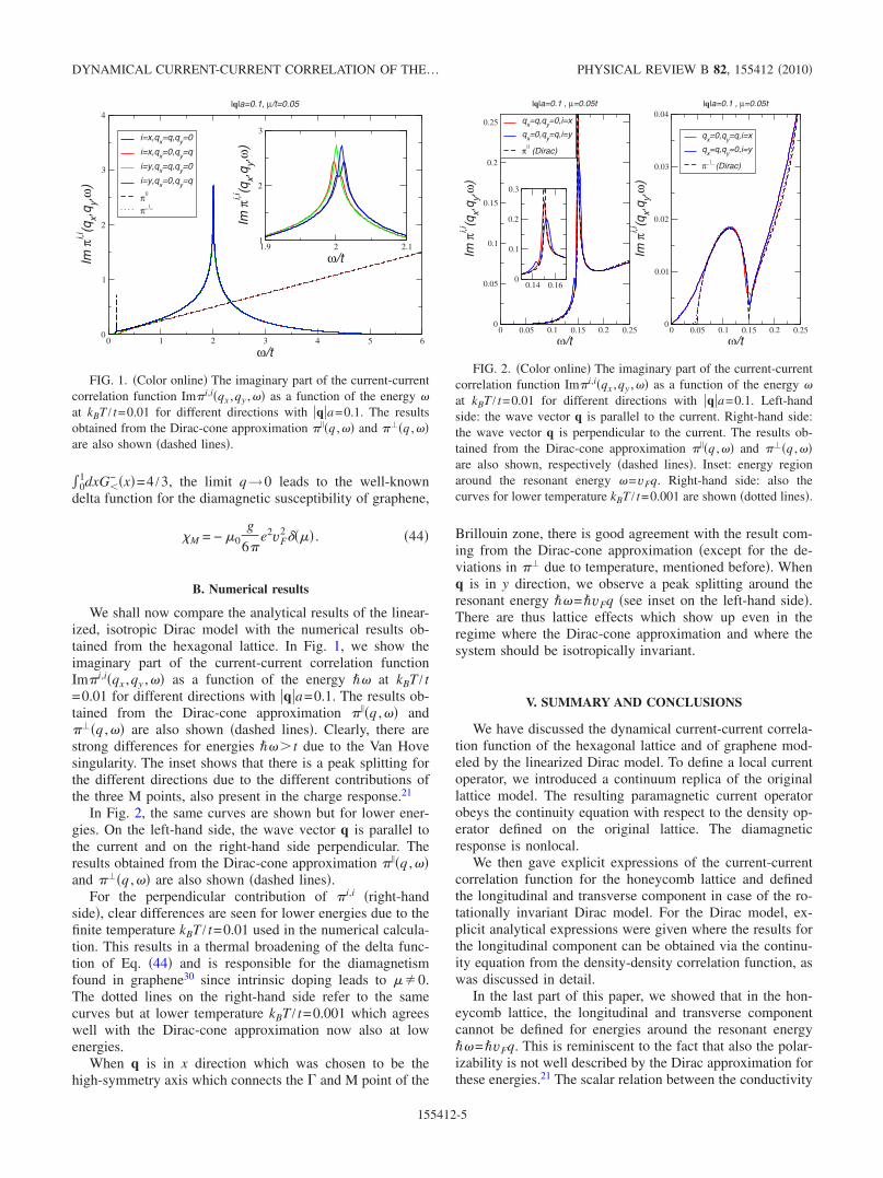
We shall now compare the analytical results of the linear-ized, isotropic Dirac model with the numerical results ob-tained from the hexagonal lattice. In Fig. 1, we show theimaginary part of the current-current correlation functionIm�i,i�qx ,qy ,�� as a function of the energy �� at kBT / t=0.01 for different directions with �q�a=0.1. The results ob-tained from the Dirac-cone approximation � �q ,�� and���q ,�� are also shown �dashed lines�. Clearly, there arestrong differences for energies ��� t due to the Van Hovesingularity. The inset shows that there is a peak splitting forthe different directions due to the different contributions ofthe three M points, also present in the charge response.21

In Fig. 2, the same curves are shown but for lower ener-gies. On the left-hand side, the wave vector q is parallel tothe current and on the right-hand side perpendicular. Theresults obtained from the Dirac-cone approximation � �q ,��and ���q ,�� are also shown �dashed lines�.

For the perpendicular contribution of �i,i �right-handside�, clear differences are seen for lower energies due to thefinite temperature kBT / t=0.01 used in the numerical calcula-tion. This results in a thermal broadening of the delta func-tion of Eq. �44� and is responsible for the diamagnetismfound in graphene30 since intrinsic doping leads to �0.The dotted lines on the right-hand side refer to the samecurves but at lower temperature kBT / t=0.001 which agreeswell with the Dirac-cone approximation now also at lowenergies.

When q is in x direction which was chosen to be thehigh-symmetry axis which connects the � and M point of the

Brillouin zone, there is good agreement with the result com-ing from the Dirac-cone approximation �except for the de-viations in �� due to temperature, mentioned before�. Whenq is in y direction, we observe a peak splitting around theresonant energy ��=�vFq �see inset on the left-hand side�.There are thus lattice effects which show up even in theregime where the Dirac-cone approximation and where thesystem should be isotropically invariant.

V. SUMMARY AND CONCLUSIONS

We have discussed the dynamical current-current correla-tion function of the hexagonal lattice and of graphene mod-eled by the linearized Dirac model. To define a local currentoperator, we introduced a continuum replica of the originallattice model. The resulting paramagnetic current operatorobeys the continuity equation with respect to the density op-erator defined on the original lattice. The diamagneticresponse is nonlocal.

We then gave explicit expressions of the current-currentcorrelation function for the honeycomb lattice and definedthe longitudinal and transverse component in case of the ro-tationally invariant Dirac model. For the Dirac model, ex-plicit analytical expressions were given where the results forthe longitudinal component can be obtained via the continu-ity equation from the density-density correlation function, aswas discussed in detail.

In the last part of this paper, we showed that in the hon-eycomb lattice, the longitudinal and transverse componentcannot be defined for energies around the resonant energy��=�vFq. This is reminiscent to the fact that also the polar-izability is not well described by the Dirac approximation forthese energies.21 The scalar relation between the conductivity

0 1 2 3 4 5 6

ω/t

0

1

2

3

4

Imπi,i

(qx,q

y,ω)

i=x,qx=q,qy=0

i=x,qx=0,qy=q

i=y,qx=q,qy=0

i=y,qx=0,qy=q

π||

π_|_

|q|a=0.1, µ/t=0.05

1.9 2 2.1

ω/t

1

2

3

Imπi,i

(qx,q

y,ω)

FIG. 1. �Color online� The imaginary part of the current-currentcorrelation function Im�i,i�qx ,qy ,�� as a function of the energy �at kBT / t=0.01 for different directions with �q�a=0.1. The resultsobtained from the Dirac-cone approximation � �q ,�� and ���q ,��are also shown �dashed lines�.

0 0.05 0.1 0.15 0.2 0.25

ω/t

0

0.05

0.1

0.15

0.2

0.25

Imπi,i

(qx,q

y,ω)

qx=q,qy=0,i=x

qx=0,qy=q,i=y

π||(Dirac)

|q|a=0.1 , µ=0.05t

0 0.05 0.1 0.15 0.2 0.25

ω/t

0

0.01

0.02

0.03

0.04

Imπi,i

(qx,q

y,ω)

qx=0,qy=q,i=x

qx=q,qy=0,i=y

π_|_(Dirac)

|q|a=0.1 , µ=0.05t

0.14 0.160

0.1

0.2

0.3

qx=q,qy=0,i=x

qx=0,qy=q,i=y

π||(Dirac)

FIG. 2. �Color online� The imaginary part of the current-currentcorrelation function Im�i,i�qx ,qy ,�� as a function of the energy �at kBT / t=0.01 for different directions with �q�a=0.1. Left-handside: the wave vector q is parallel to the current. Right-hand side:the wave vector q is perpendicular to the current. The results ob-tained from the Dirac-cone approximation � �q ,�� and ���q ,��are also shown, respectively �dashed lines�. Inset: energy regionaround the resonant energy �=vFq. Right-hand side: also thecurves for lower temperature kBT / t=0.001 are shown �dotted lines�.

DYNAMICAL CURRENT-CURRENT CORRELATION OF THE… PHYSICAL REVIEW B 82, 155412 �2010�

155412-5

and the polarizability which makes use of the fact that thereis a parallel component does thus not hold for the latticemodel. This might be important for first-principles studieswhich make use of this relation.

ACKNOWLEDGMENTS

This work has been supported by FCT under grantPTDC/FIS/101434/2008 and MCI under grant FIS2010-21883-C02-02.

APPENDIX: REAL EXPRESSIONS FOR THE CURRENT-CURRENT CORRELATION FUNCTION

Here, we shall present the real and imaginary part of ���

in terms of the three real dimensionless functions

f��q,�� =g

16�

��

t�1 − vFq

��2��1/2

,

G���x� = x�x2 − 1 � cosh−1�x�, x � 1,

G���x� = � x�1 − x2 − cos−1�x�, �x� � 1. �A1�

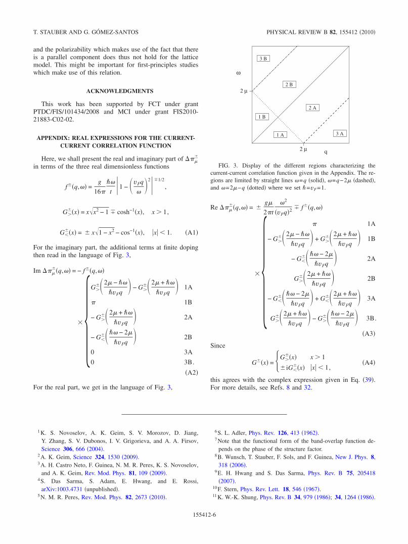
For the imaginary part, the additional terms at finite dopingthen read in the language of Fig. 3,

Im ����q,�� = − f��q,��

��G�

�2 − ��

�vFq� − G�

�2 + ��

�vFq� 1A

� 1B

− G��2 + ��

�vFq� 2A

− G���� − 2

�vFq� 2B

0 3A

0 3B.

��A2�

For the real part, we get in the language of Fig. 3,

Re ����q,�� = �

g

2�t

�2

�vFq�2 � f��q,��

��� 1A

− G��2 − ��

�vFq� + G�

�2 + ��

�vFq� 1B

− G���� − 2

�vFq� 2A

G��2 + ��

�vFq� 2B

− G���� − 2

�vFq� + G�

�2 + ��

�vFq� 3A

G��2 + ��

�vFq� − G�

��� − 2

�vFq� 3B.

��A3�

Since

G��x� = �G���x� x � 1

�iG���x� �x� � 1,

� �A4�

this agrees with the complex expression given in Eq. �39�.For more details, see Refs. 8 and 32.

1 K. S. Novoselov, A. K. Geim, S. V. Morozov, D. Jiang,Y. Zhang, S. V. Dubonos, I. V. Grigorieva, and A. A. Firsov,Science 306, 666 �2004�.

2 A. K. Geim, Science 324, 1530 �2009�.3 A. H. Castro Neto, F. Guinea, N. M. R. Peres, K. S. Novoselov,

and A. K. Geim, Rev. Mod. Phys. 81, 109 �2009�.4 S. Das Sarma, S. Adam, E. Hwang, and E. Rossi,

arXiv:1003.4731 �unpublished�.5 N. M. R. Peres, Rev. Mod. Phys. 82, 2673 �2010�.

6 S. L. Adler, Phys. Rev. 126, 413 �1962�.7 Note that the functional form of the band-overlap function de-

pends on the phase of the structure factor.8 B. Wunsch, T. Stauber, F. Sols, and F. Guinea, New J. Phys. 8,

318 �2006�.9 E. H. Hwang and S. Das Sarma, Phys. Rev. B 75, 205418

�2007�.10 F. Stern, Phys. Rev. Lett. 18, 546 �1967�.11 K. W.-K. Shung, Phys. Rev. B 34, 979 �1986�; 34, 1264 �1986�.

2 µ

2 µ

ω

q

3 A

2 A

1 A

1 B

2 B

3 B

FIG. 3. Display of the different regions characterizing thecurrent-current correlation function given in the Appendix. The re-gions are limited by straight lines �=q �solid�, �=q−2 �dashed�,and �=2−q �dotted� where we set �=vF=1.

T. STAUBER AND G. GÓMEZ-SANTOS PHYSICAL REVIEW B 82, 155412 �2010�

155412-6

12 J. González, F. Guinea, and M. A. H. Vozmediano, Phys. Rev. B59, R2474 �1999�.

13 T. Ando, J. Phys. Soc. Jpn. 75, 074716 �2006�.14 O. Vafek, Phys. Rev. Lett. 97, 266406 �2006�.15 S. Gangadharaiah, A. M. Farid, and E. G. Mishchenko, Phys.

Rev. Lett. 100, 166802 �2008�.16 M. R. Ramezanali, M. M. Vazifeh, R. Asgari, M. Polini, and

A. H. MacDonald, J. Phys. A: Math. Theor. 42, 214015 �2009�.17 R. Roldán, J.-N. Fuchs, and M. O. Goerbig, Phys. Rev. B 80,

085408 �2009�.18 P. K. Pyatkovskiy, J. Phys.: Condens. Matter 21, 025506 �2009�.19 T. G. Pedersen, A.-P. Jauho, and K. Pedersen, Phys. Rev. B 79,

113406 �2009�.20 A. Hill, S. A. Mikhailov, and K. Ziegler, EPL 87, 27005 �2009�.21 T. Stauber, J. Schliemann, and N. M. R. Peres, Phys. Rev. B 81,

085409 �2010�.22 T. Tudorovskiy and S. A. Mikhailov, Phys. Rev. B 82, 073411

�2010�.23 M. van Schilfgaarde and M. Katsnelson, arXiv:1006.2426

�unpublished�.24 R. A. Muniz, H. P. Dahal, A. V. Balatsky, and S. Haas, Phys.

Rev. B 82, 081411�R� �2010�.25 D. Gazit, Phys. Rev. B 79, 113411 �2009�.26 J. F. Dobson, A. White, and A. Rubio, Phys. Rev. Lett. 96,

073201 �2006�; G. Gómez-Santos, Phys. Rev. B 80, 245424�2009�.

27 K. F. Allison, D. Borka, I. Radovic, L. Hadzievski, and Z. L.

Miskovic, Phys. Rev. B 80, 195405 �2009�.28 J. W. McClure, Phys. Rev. 104, 666 �1956�.29 M. Koshino, Y. Arimura, and T. Ando, Phys. Rev. Lett. 102,

177203 �2009�.30 M. Sepioni, S. Rablen, R. Nair, J. Narayanan, F. Tuna, R. Win-

penny, A. K. Geim, and I. Grigorieva, arXiv:1007.0423 �unpub-lished�.

31 A. Principi, M. Polini, G. Vignale, and M. I. Katsnelson, Phys.Rev. Lett. 104, 225503 �2010�.

32 A. Principi, M. Polini, and G. Vignale, Phys. Rev. B 80, 075418�2009�.

33 X.-G. Wen, Quantum Field Theory of Many-Body Systems �Ox-ford University Press, New York, 2004�.

34 I. Paul and G. Kotliar, Phys. Rev. B 67, 115131 �2003�.35 D. J. Scalapino, S. R. White, and S. C. Zhang, Phys. Rev. B 47,

7995 �1993�.36 V. P. Gusynin, S. G. Sharapov, and J. P. Carbotte, Phys. Rev. B

75, 165407 �2007�.37 N. M. R. Peres and T. Stauber, Int. J. Mod. Phys. B 22, 2529

�2008�; T. Stauber, N. M. R. Peres, and A. K. Geim, Phys. Rev.B 78, 085432 �2008�.

38 C. Bena and G. Montambaux, New J. Phys. 11, 095003 �2009�.39 J. Sabio, J. Nilsson, and A. H. Castro Neto, Phys. Rev. B 78,

075410 �2008�.40 S. A. Mikhailov and K. Ziegler, Phys. Rev. Lett. 99, 016803

�2007�.

DYNAMICAL CURRENT-CURRENT CORRELATION OF THE… PHYSICAL REVIEW B 82, 155412 �2010�

155412-7