Dynamics and Control of a Planar MultibodyMobile Robot for Confined Environment

Inspection

Lounis DouadiSchool of Electrical Engineering

and Computer ScienceUniversity of Ottawa

Email: ldouadi@uottawa.ca

Davide Spinello∗

Department of Mechanical EngineeringUniversity of Ottawa

Email: dspinell@uottawa.ca

Wail GueaiebSchool of Electrical Engineering

and Computer ScienceUniversity of Ottawa

Email: wgueaieb@eecs.uottawa.ca

ABSTRACTIn this paper, we study the dynamics of an articulated planar mobile robot for confined

environment exploration. The mobile vehicle is composed of n identical modules hitched togetherwith passive revolute joints. Each module has the structure of a four-bar parallel mechanismon a mobile platform. The dynamic model is derived using Lagrange formulation. Computersimulations illustrate the model by addressing a path following problem inside a pipe. Thedynamic model presented in this paper is the basis for the design of motion control algorithmsthat encode energy optimization and sensor performance maximization.

1 Introduction and Related LiteratureThis work is part of a project aimed at the development of a three-dimensional autonomous articu-

lated mobile robot for the exploration and nondestructive testing in confined environments that can behazardous or not accessible to humans. One application targeted by this system is natural gas pipelinesinspection. Articulated mobile robots made their appearance in the framework of service robotics [1].Snake-like mobile robots are often chosen for the class of applications we are interested in because oftheir great agility and high redundancy, which enable them to operate in environments that might betoo challenging for a conventional wheeled robot. For instance, they are conveniently deployed insidepipelines [2], in narrow spaces, and on the rubble of an earthquake or a major fire, and find applica-tions in fields as diverse as rescue operations, military/defense, and confined environment explorationas, for example, inspection of bridges [3], inspection of natural gas pipelines, industrial pipes and sewerpipelines [4–9], to name a few. Snake-like robots proposed in the literature are typically locomotedeither with passive caster wheels supporting their frames [10–12] or with no wheels at all [13–16].

∗Address all correspondence to this author.

1

For service applications such as inspection and maintenance in confined, not accessible, and eventu-ally hazardous environments it is crucial to equip the robot with decision making and control algorithmsthat, among other features, maximize the time in which the robot can operate autonomously. Thisrequires the development of dynamic models that account for salient features of the system, and there-fore be able to formulate with relatively high accuracy the control efforts involved in typical operatingscenarios [17,18]. In this way one can optimize the energy consumption and eventually the sensors per-formance, which is a metric to measure the quality of the inspection and eventual detection of defectsand other features. In [19] it is investigated the static and stiffness model of serial-parallel manipulators.In [20] the dynamic model of an articulated vehicle consisting of one car-like tractor and two cart-likesemi-trailers is developed using the Newton-Euler equations with the constraint of no slippage. The dy-namics of the snake-like robot SES-1 with high speed and high efficiency locomotion is derived in [21].Transeth et al. [22, 23] presented a three-dimensional wheel-less snake-like robot modeled using non-smooth dynamics and convex analysis for the incorporation of contact and friction forces. The authorsderived a simplified model of planar snake robot locomotion in [24] based on Newton’s formulation.The simplification is obtained by considering the body shape changes of the snake robot as linear dis-placements of the links with respect to each other instead of rotational displacements. A hybrid modelof the dynamics of a planar snake robot interacting with obstacles is derived in [25]. The concept ofequality of measures is used in [26] to describe the dynamics of a planar snake-like robot while a newdynamic modeling method for snake-like robots using the concept of Nominal Mechanism is introducedin [27]. A recent survey on snake-like robots modeling is given in [28]. The common point betweenthese models is that they deal with the dynamics of multibody systems [29]. Multibody dynamics mod-eling and simulation has applications in robotics, biomechanics, and virtual reality among others. Themajor difficulty in modeling multibody systems is the systematic enforcement of internal and externalkinematic constraints.

Here, we consider the model of a multibody articulated robot composed of a sequence of modulesin plane motion hitched together with passive joints. Each module is a parallel robot on a mobile plat-form, where a body standing for a payload is supported by two arms with one extremity in contactwith the walls of the environment in which the robot operates. The mechanism proposed here is char-acterized by a higher number of degrees of freedom as compared to other articulated robots, such asthe n-trailer system, that are often adopted for similar applications. The augmented number of mini-mal coordinates and increased robot’s dexterity and maneuverability inside the pipeline may be crucialin executing some pipe inspection maneuvers. A larger number of available control inputs implies in-deed increased versatility in operations that involve for example turning relatively sharp elbows whilemaintaining the modules centered for the purpose of maximizing sensor performances. We derive thedynamics of the system by considering the Lagrangian formulation, which allows to easily include theinternal constraints and it is therefore useful to systematically treat multibody systems. We introduce anon-minimum coordinates set along with a suitable set of constraints stating the couplings among coor-dinates. The constrained equations of motion form a system of differential algebraic equations. Manymethods to solve those equations can be found in the literature [30,31]. We use the method that throughdifferentiation transforms the constraints into second order equations. The shortcoming of this methodis that the constraints are enforced at the acceleration level and therefore it is necessary to explicitlycheck that the corresponding velocity and/or position constraints are satisfied. This motivates workson constraint stabilization [32–34], constraints enforcement and constraint elimination. A survey onspecial techniques to enforce constraints can be found in [35].

The rest of the paper is organized as follows. In Section 2, we present the structure of the robot. Thekinematics is discussed in Section 3, along with singular configurations of the modules. The dynamicsand the derivation of the equations of motion of the system are presented in Section 4. The model isillustrated through the simulation of path following control inside a pipe in Section 5. Section 6 is left

2

for conclusions.

2 The Articulated Mobile Robot and The Geometric Description of The WorkspaceIn this section, we briefly describe the structural architecture of the robot and the environment in

which it operates. As sketched in Figure 1, the vehicle is composed of n identical modules, each forminga closed kinematic chain moving in a connected region Ω ∈ R2. The leading and terminal modules M1and Mn are called respectively the head and the tail of the robot. The modules are hitched together byn−1 passive revolute joints. The name convention for these joints is such that joint Pi connects modulesMi−1 and Mi with i = 2 . . .n. The vehicle is propelled by n pairs of horizontal active wheels, that are incontact with the walls. In simulation, the contact is enforced by a suitable set of Lagrange multipliersthat represent the contact forces between the wheels and the walls. By considering a single module asshown in the schematics of Figure 6, the mechanism can be treated as a closed kinematic chain on amobile platform. It is similar to a four-bar linkage with the particularity of having mobile bases sincethe wheels move independently from each other along two curves representing the boundaries of theconfined environment. This adds two degrees of freedom as compared to the one-degree-of-freedomfour-bar linkage. Hence, a module Mi, when disconnected, has three degrees of freedom.

A pair of points P and Q in Ω is mapped into the vector rPQ by the difference

Q−P = rPQ (1)

defined as in the usual framework of affine spaces. By referring the space to a global Cartesian referenceframe O,ex,ey, with origin O and unit vectors ex and ey, the difference P−O is the position vectorrOP with representation

rOP = xPex + yPey (2)

in the global frame. By referring to Figure 6, h and W are respectively the height and the width of themodule; γ is a nondimensional parameter that represents the fraction of the height of the main body atwhich the arms are pinned; L is the length of the arms; and θi, αr

i and αli are respectively the orientation

angle of the module, and the right and left relative joint angles of the right and left shoulder joints. Eachpin connecting two modules corresponds to two scalar constraints. For a vehicle with n modules (seeFigure 1) the total number of degrees of freedom is 3n−2(n−1) = n+2.

In a two-dimensional setting, the right and the left walls of the pipeline are described by the para-metric curves ΠΠΠ

r and ΠΠΠl respectively. Parametric curves evaluated at the arclength sr and sl map to

points in the plane, that with a slight abuse of notation can be expressed as position vectors in the globalframe O,ex,ey

ΠΠΠr(sr) = Π

rx(s

r)ex +Πry(s

r)ey (3)

ΠΠΠl(sl) = Π

lx(s

l)ex +Πly(s

l)ey (4)

with the implicit understanding that position vectors and related Cartesian coordinates Πlx,Π

ly and

Πrx,Π

ry are referred to the origin O. The Frenet frames Tr,Nr and Tl,Nl associated to the para-

metric curves are defined in terms of the tangent and normal vectors as

Tr =dΠΠΠ

r

dsr =dΠr

xdsr ex +

dΠry

dsr ey =: T rx ex +T r

y ey (5a)

3

Nr =1κr

dTr

dsr =1κr

(d2Πr

x

dsr2 ex +d2Πr

y

dsr2 ey

)=: Nr

xex +Nryey (5b)

where we have introduced the Cartesian components T rx ,T

ry and Nr

x ,Nry of the tangent and of the

normal fields to the right wall, and the curvature κr. By replacing the superscript r with l the corre-sponding Frenet frame for the left wall is obtained.

3 Kinematics3.1 Configuration Kinematics

Since each module is a closed kinematic chain, the position of the center of mass can be equivalentlyexpressed by the following vector relations, see Figure 6

rOGi = rOCri+ rCr

i Bri+ rBr

i Sri+ rSr

i Gi (6a)

rOGi = rOCli+ rCl

i Bli+ rBl

iSli+ rSl

iGi(6b)

where Sli and Sr

i are the points defining the left and right shoulders (arms are attached to the body); Cri

and Cli are the points on the right and left wheels that are closest to the related walls; Br

i and Bli are the

centers of the wheels; and Gi is the center of mass of the body of the module Mi. The position of thecenter of mass Gi is expressed in the global reference frame as

rOGi = xGiex + yGiey (7)

For each module, we introduce the following rotated basis, that has the meaning of a body referenceframe

(Eix Eiy) = (ex ey)R(θi) (8)

where R is the rotation matrix

R(θi) =

(cosθi −sinθisinθi cosθi

)(9)

In this basis, vectors in (6) are expressed as

rSri Gi =−HEix +

W2

Eiy (10a)

rBri Sr

i= LR(αr

i )Eix (10b)

rSliGi

=−HEix−W2

Eiy (10c)

rBliS

li=−LR(αl

i)Eix (10d)

where H = h(γ−1/2). By using the orthogonality of R we express the relative position vectors in theglobal reference frame as

rSri Gi =

(−W

2sinθi−H cosθi

)ex

4

+

(W2

cosθi−H sinθi

)ey (11a)

rBri Sr

i= L(cos(θi +α

ri )ex + sin(θi +α

ri )ey) (11b)

rSliGi

=

(W2

sinθi−H cosθi

)ex

+

(−W

2cosθi−H sinθi

)ey (11c)

rBliS

li=−L

(cos(

θi +αli

)ex + sin

(θi +α

li

)ey

)(11d)

Since the wheels are circular, the minimum distance with the walls is achieved at the point Cri (Cl

i ),such that the tangent to the wheel at the same point is parallel to Tr(sr

i ) (Tl(sli)), respectively, where sr

i(sl

i) is the corresponding arclength. Therefore the line joining Cri (Cl

i ) and its projection to the wall isdirected as the normal Nr(sr

i ) (Nl(sli)), see Figure 3. The relative position vectors rCr

i Bri

and rCli B

li

in (6)are therefore given by

rCri Br

i= ρNr(sr

i )

=(xBr

i(sr

i )− xCri(sr

i ))

ex +(yBr

i(sr

i )− yCri(sr

i ))

ey (12a)

rCli B

li=−ρNl(sl

i)

=(

xBli(sl

i)− xCli(sl

i))

ex +(

yBli(sl

i)− yCli(sl

i))

ey (12b)

where ρ is the radius of the wheels. The characterization of position vectors in (6) is completed by

rOCri= ΠΠΠ

r(sri )+ rΠΠΠ

r(sri )C

ri

(13a)

rOCli= ΠΠΠ

l(sli)+ r

ΠΠΠl(sl

i)Cli

(13b)

where rΠΠΠr(sr

i )Cri

and rΠΠΠ

l(sli)C

li

are gap vectors. Here we set the gap to be zero, which corresponds to contactwheels to walls. This condition can be violated by geometric incompatibility between the robot and thewalls, as for example in case of sharp turns not compatible with the length of the modules, or whenthe walls have geometric singularities as corners that cannot be negotiated smoothly. The second casehas been studied in [36], and an optimal control on a modified module with extensible arms has beenproposed to navigate across the corner while avoiding singularities. In terms of position kinematics, thecontact condition implies

rOBri= rOCr

i+ rCr

i Bri= ΠΠΠ

r(sri )+ρNr(sr

i )

= xBri(sr

i )ex + yBri(sr

i )ey (14a)

rOBli= rOCl

i+ rCl

i Bli= ΠΠΠ

l(sli)−ρNl(sl

i)

= xBli(sl

i)ex + yBli(sl

i)ey (14b)

Substituting from (14) and (11) into (6), and by projecting along ex and ey we obtain the geometric

5

closure equations of the module’s mechanism

xGi− xBri(sr

i )+H cosθi +W2

sinθi−Lcos(θi +αri ) = 0 (15a)

yGi− yBri(sr

i )+H sinθi−W2

cosθi−Lsin(θi +αri ) = 0 (15b)

xGi− xBli(sl

i)+H cosθi−W2

sinθi +Lcos(θi +αli) = 0 (15c)

yGi− yBli(sl

i)+H sinθi +W2

cosθi +Lsin(θi +αli) = 0 (15d)

The geometric relation between the wheels and the arms to which they are attached is expressed bythe following relations

rOAri+ rAr

i Bri= rOBr

i(16a)

rOAli+ rAl

iBli= rOBl

i(16b)

where Ari and Al

i are the centers of mass of the right and of the left arms. The relative vectors in theglobal basis are given by

rAri Br

i=−L

2R(αr

i )Eix

=−L2(cos(θi +α

ri )ex + cos(θi +α

ri )ey) (17a)

rAliB

li=

L2

R(αli)Eix

=L2

(cos(θi +α

li)ex + sin(θi +α

li)ey

)(17b)

By substituting into (16) and by projecting on the global basis the following set of four scalar constraintsis obtained

xAri− xBr

i− L

2cos(θi +α

ri ) = 0 (18a)

yAri− yBr

i− L

2sin(θi +α

ri ) = 0 (18b)

xAli− xBl

i+

L2

cos(

θi +αli

)= 0 (18c)

yAli− yBl

i+

L2

sin(

θi +αli

)= 0 (18d)

for i = 1, . . . ,n, where xAri, yAr

i, xAl

iand yAl

iare the global coordinates of the centers of mass of the right

and left arms respectively.The connection of two modules Mi−1 and Mi by a revolute joint is expressed by constraints formal-

izing the contact at point Pi, see Figure 1

rOGi−1 + rGi−1Pi = rOGi + rGiPi (19)

6

In the global reference frame the relative position vectors are given by

rGi−1Pi =−LbR(θi−1)Ei−1x

=−Lb (cosθi−1ex + sinθi−1ey) (20a)rGiPi = L f R(θi)Eix

= L f (cosθiex + sinθiey) (20b)

with Lb = ‖rGi−1Pi‖ and L f = ‖rGiPi‖ (see Figure 1). Substitution into (19) gives the scalar positionconstraints

xGi−1− xGi−Lb cosθi−1−L f cosθi = 0 (21a)yGi−1− yGi−Lb sinθi−1−L f sinθi = 0 (21b)

for i = 1, . . . ,n−1.

3.2 Velocity KinematicsTime differentiating equations (15) we obtain the tangent closure kinematic equations

xGi +ari θi− xBr

i− cr

i αri = 0 (22a)

yGi +bri θi− yBr

i−dr

i αri = 0 (22b)

xGi +ali θi− xBl

i− cl

iαli = 0 (22c)

yGi +bli θi− yBl

i−dl

i αli = 0 (22d)

for i = 1, . . . ,n, where ari , br

i , cri , dr

i and the analogous for the left arm are configuration-dependentparameters listed in the Appendix.

In the velocity space, the permanent contact between the wheels and the walls is formalized byrolling without slipping constraints, which state that the relative velocity between the walls and thecontact point is zero:

rΠΠΠr(sr

i )Cri= 0 (23a)

rΠΠΠ

l(sli)C

li= 0 (23b)

We assume that the walls are at rest, which implies that the absolute velocities rOCri

and rOCli

of thepoints in contact with the walls are zero. By using the rigid body velocity transformation we obtain

rOCri= rOBr

i+ωωω

rwi ∧ rBr

iCri= 0 (24a)

rOCli= rOBl

i+ωωω

lwi ∧ rBl

iCli= 0 (24b)

where rOBri

and rOBli

are the absolute velocities of the centers of mass of the wheels, ωωωrwi and ωωωlw

i arethe angular velocities, and “∧” is the exterior (cross) product. By using the representations in (12), the

7

projection of (24) on the global basis gives the scalar rolling without slipping relations

xBri+ρω

rwi Nr

y(sri ) = 0 (25a)

yBri−ρω

rwi Nr

x(sri ) = 0 (25b)

xBli−ρω

lwi Nl

y(sli) = 0 (25c)

yBli+ρω

lwi Nl

x(sli) = 0 (25d)

for i = 1, . . . ,n. We note that the rolling without slipping constraint implies that the two components ofthe absolute velocity of the contact points are zero (since the walls are at rest). Therefore, by choosingan initial configuration in which the wheels are in contact with the walls, this constraint is sufficient toensure that they remain in contact as the system evolves. Since the angular velocity vectors are normalto the plane of the position vectors, the cross products in (24) can be written in terms of the Frenetframes as

ωωωrwi ∧ rBr

iCri= ωωω

rwi ∧ (−ρNr) = ρω

rwi Tr (26a)

ωωωlwi ∧ rBl

iCli= ωωω

lwi ∧ρNl =−ρω

lwi Tl (26b)

Moreover, time differentiating expressions in (14), and by using the second Frenet-Serret formula weobtain

rOBri= ΠΠΠ

r(sr

i )+ρNr(sri ) = sr

i Tr(sr

i )−ρsri κ

rTr(sri ) (27a)

rOBli= ΠΠΠ

l(sl

i)−ρNl(sli) = sl

iTl(sl

i)+ρsliκ

lTl(sli) (27b)

which shows that rolling without slipping constraints imply that velocities of the center of mass of thewheels are parallel to the tangent to the wall at the contact points. By combining (27), (26), and (24)we obtain the following relations between the wheels angular velocities and the rate of change of thearclength parameters

sri =−

ρ

1−ρκr ωrwi (28a)

sli =

ρ

1+ρκl ωlwi (28b)

Therefore the change of arclength and the angular velocity can be considered, from a kinematic per-spective, as driving parameters of the system. The rate of change of the arclength parameters can beregarded as the speed of the wheel’s center of mass, that by virtue of the rolling without slipping con-straints is related to the angular velocity. When the curvature of the wall is zero the expressions in (28)give the expected relations between angular velocity, forward speed of the center of mass, and radius ofthe wheel. If the radius of curvature of the wall, 1/κ, is larger than the radius of curvature of the wheel,ρ, then s and ω are consistent with respect to the forward motion of the mechanism; if the radius ofcurvature of the wall is smaller than the radius of curvature of the wheel then s and ω are not consistentwith respect to the forward motion, which means that a forward angular velocity (with respect to themotion) of the wheel corresponds to backward linear velocity (with respect to the motion) of its center

8

of mass. Therefore scenarios that involve walls with large curvature require special attention. Note thatthe signs in (28) account for the fact that, with respect to forward motion, the inner part of the pipelineis to the right of ΠΠΠ

l and to the left of ΠΠΠr.

The set of velocity constraints associated to each module is completed by differentiating (18) intime, to obtain the wheel to arm pinning condition in the velocity space:

xBri− xAr

i− L

2(θi + α

ri)

sin(θi +αri ) = 0 (29a)

yBri− yAr

i+

L2(θi + α

ri)

cos(θi +αri ) = 0 (29b)

xBli− xAl

i+

L2(θi + α

li)sin(θi +α

li) = 0 (29c)

yBli− yAl

i− L

2(θi + α

li)cos(θi +α

li) = 0 (29d)

The velocity constraints that express the connection between two modules are obtained by differen-tiating (21) in time

xGi−1− xGi +Lbθi−1 sinθi−1 +L f θi sinθi = 0 (30a)

yGi−1− yGi−Lbθi−1 cosθi−1−L f θi cosθi = 0 (30b)

for i = 1, . . . ,n−1.We adopt the following nonminimal set of joint coordinates qi and set of end effector coordinates pi

(here we use the term end effector to refer to the platform of the mechanism)

qi =[xBr

i,yBr

i,xBl

i,yBl

i,αr

i ,αli,θ

ri ,θ

li,xAr

i,yAr

i,xAl

i,yAl

i

](31a)

pi = [xGi,yGi,θi] (31b)

where θri and θl

i are the angular coordinates of the wheels. By collectively expressing equations (22),(25), and (29) we rewrite the systems in matrix form as

Jpi pi = Jqi qi (32)

where Jpi ∈ R12×3 and Jqi ∈ R12×12 are, respectively, the parallel and the serial Jacobians of the mech-anism and are given in the Appendix.

For a vehicle with n modules, let p = [p1 . . . pn]T ∈ R3n be the collection of operational coordinates

and q = [q1 . . .qn]T ∈ R12n be the collection of joint coordinates. The collective velocity kinematics of

the multibody mechanism that include the hitching constraints (30) is therefore written as

Jp p = Jqq (33)

with Jacobians Jp ∈ R(14n−2)×3n and Jq ∈ R(14n−2)×12n given in the Appendix. Note that the couplingbetween modules is included in Jp.

For the system of n modules with n− 1 joints we have therefore 12n+ 2(n− 1) constraints amongwhich 12n describe the inner connections among parts of the individual modules (equations (22) and

9

(29)) and the rolling without slipping constraint (equations (25)), while the remaining 2n− 2 describehitching constraints (equations (30)). The total number of kinematic constraints is therefore 14n−2 for15n unknowns (3n Cartesian velocities and 12n joint velocities). This leaves n+2 degrees of freedom,which is the dimension of a minimal set of coordinates for the articulated vehicle. For instance, one canchoose position and orientation of the head and the n−1 orientations, one for each remaining modules.

3.3 SingularitiesSingularities occur when one or both Jacobians, Jp and Jq, become singular [37]. A parallel singu-

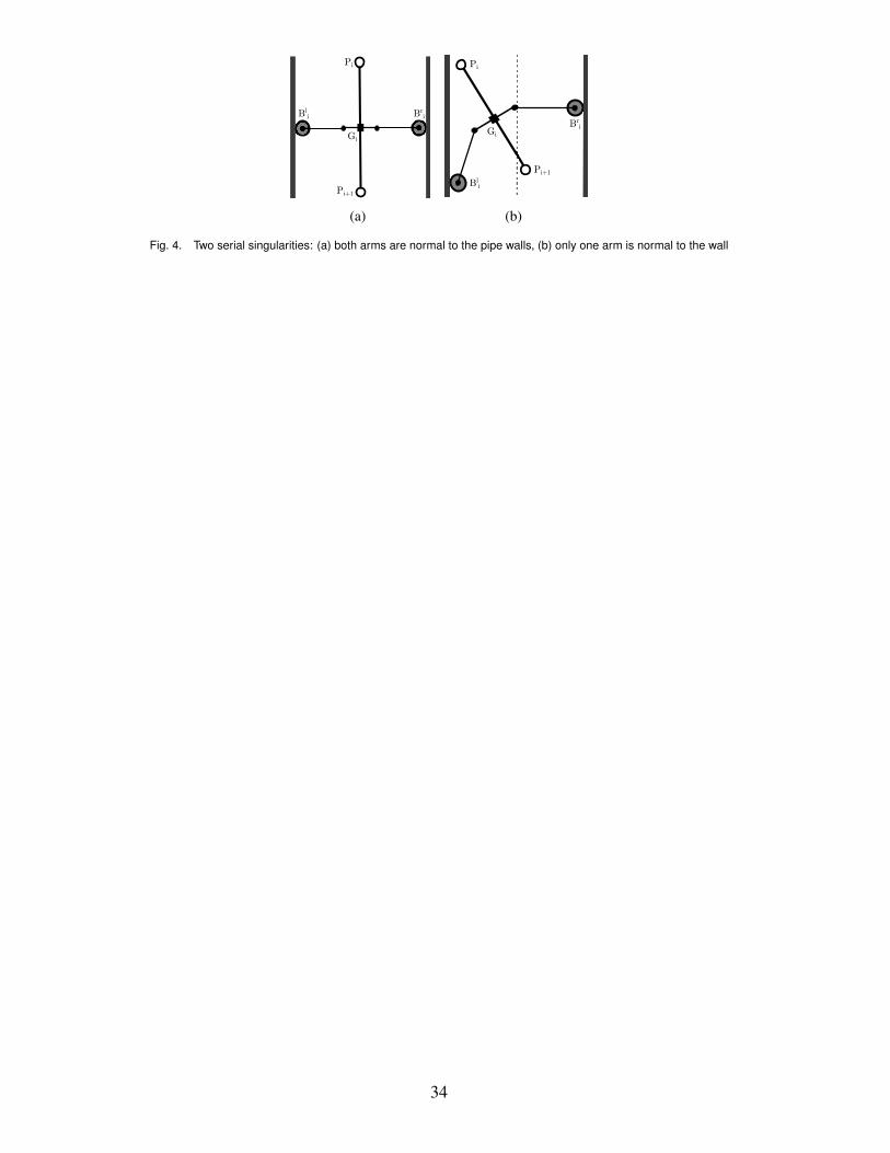
larity occurs when the parallel Jacobian Jp takes a singular value, and a serial singularity occurs whenthe serial Jacobian Jq is singular, corresponding to configurations where the robot loses one or moredegrees of freedom [38]. For a single module Mi, a serial singularity occurs when detJqi = 0. Thisimplies

Nlx(s

li)sin(θi +α

li) = Nl

y(sli)cos(θi +α

li) (34)

orNr

x(sri )sin(θi +α

ri ) = Nr

y(sri )cos(θi +α

ri ). (35)

These conditions correspond to configurations where one or both arms of the module are normal to thecorresponding pipe wall. Figure 4 illustrates two examples of such cases. The singular position depictedin figure 4(a) occurs when each arm is perpendicular to the surface it is in contact with. It can be easilyavoided by having the mechanism’s span to be larger than the pipe diameter. Nevertheless, serial singularconfigurations as in figure 4(b) are still physically possible. Avoiding them can be encoded as part ofthe controller’s objectives [36].

Parallel singularities occur when the parallel Jacobian Jp is singular, or if it is not of full rank fora non-square Jacobian. For a single module Mi, we study the rank of Jpi through the eigenvalues ofmatrix JTpiJpi based on the fact that the singular values of Jpi are the square roots of the eigenvalues ofJTpiJpi, and by using the fact that the rank of Jpi equals the number of its nonzero singular values [39].

If det(

JTpiJpi

)6= 0, then all its eigenvalues are non-zero, and therefore all the singular values of Jpi are

non-zero, which implies that Jpi is full rank. The determinant of JTpiJpi may be expressed as

det(

JTpiJpi

)=

W 2 +2L2(

1+ cos(αri −α

li))+2WL

(sinα

ri + sinα

li

). (36)

This determinant vanishes when αri −αl

i = π and W = 0. Figure 5 depicts a configuration correspondingto those conditions. We assume that the module width W is nonzero. A way to avoid parallel singular-ities is to set the constraints 0 < αr

i <π

2 and π

2 < αli < π on the shoulder joints, so that the determinant

never vanishes.

4 Dynamics4.1 Equations of Motion

In this section, we present the dynamics and derive the equations of motion of the system. Asdiscussed in previous sections, each module is a multibody system comprising the main body standingfor the payload, two arms and two wheels. The equations of motion of the system are derived based

10

on Lagrange’s formulation. For each module, we use the non-minimal set of coordinates ξTi = [pTi ,qTi ],

with ξi ∈ R15 and pi and qi defined in (31). Constraints (22), (25) and (29) are accounted for throughLagrange multipliers. The Lagrangian function Li(ξi) of module Mi reduces to its kinetic energy Ti(ξi)since we consider a planar system with no potential fields. Contributions to the Lagrangian can beexplicitly identified as the individual contributions of the kinetic energies of the parts composing amodule

Li = T bi +T ra

i +T lai +T rw

i +T lwi (37)

where T bi , T ra

i , T lai , T rw

i , and T lwi are respectively the kinetic energy of the main body (payload or

end effector), right arm, left arm, right wheel and left wheel. As illustrated in Figure 6, we consider themain body to be rectangular with mass m, the arms as rods of identical mass ma, and the wheels as discswith identical mass mw. Therefore the kinetic energies written in terms of translational and rotationalcontributions are given by

T bi =

12

rGi ·mrGi +12

Ibθ2i (38a)

T rai =

12

rAri·marAr

i+

12

ωωωrai · Iaωωω

rai (38b)

T rwi =

12

rBri·mwrBr

i+

12

ωωωrwi · Iwωωω

rwi (38c)

where “·” is the inner product; rGi , rAri, and rBr

iare the velocities of the centers of mass of the body, right

arm, and right wheel (analogous expressions can be obtained for the left arm and wheel by renamingthe superscript from r to l); ωωωra

i is the angular velocity of the right arm (normal to the plane definedby the linear velocities); and Ib, Ia, and Iw are respectively polar moments of inertia of the main body,right arm, and right wheel about their own centers of mass. Kinetic energy expressions for the left armand left wheel are obtained by changing the superscript r to l in (38). By using the law of compositionof angular velocities (see for example [40, Chapter 4]) and by recalling that αr

i is the relative angularposition of the arm with respect to the body, the angular velocity of the arm can be written as

ωωωrai = θiez + α

ri ez (39)

where ez is the unit normal to the plane of the motion. By projecting vectors in (38) in the orthonormalbasis ex,ey,ez we obtain the expressions for the kinetic energies in terms of the adopted set of non-minimal coordinates

T bi =

12

m(x2

Gi+ y2

Gi

)+

12

Ibθ2i (40)

T rai =

12

ma

(x2

Ari+ y2

Ari

)+

12

Ia(α

ri + θi

)2 (41)

T rwi =

12

mw

(x2

Bri+ y2

Bri

)+

12

Iwωrwi

2 (42)

Given the dynamics of one module, we can derive the dynamics of the articulated mobile robotby incorporating the constraints relating adjacent modules. Hitching n modules together results in a

11

more complex constrained multibody system. We define the state vector ξ = [ξ1, . . . ,ξn] ∈ R15n, that isnon-minimal as the number of degrees of freedom of the mechanism is n+2.

In order to derive the equations of motion for the multibody system composed of n modules, weconsider the Lagrangian of the articulated vehicle that is the sum of Lagrangians of the n modules

L(ξ) =n

∑i=1

Li(ξi) =n

∑i=1

Ti(ξi) (43)

Since we have chosen a set of nonminimal coordinates that allows us to easily write the kinetic energies,the 12n constraints (12 for each module) (22), (25), and (29) and the 2(n−1) hitching constraints (30)must be included in the Lagrangian formulation, for the total number of velocity constraints given by12n+2(n−1) = 14n−2. We collectively express them in matrix form by

Cξ = 0 (44)

where C ∈ R(14n−2)×15n is the velocity constraint Jacobian of the multibody system, that is given by

C =

J1Q1 S2

J2 0Q2 S3

. . .0 Jn−1

Qn−1 SnJn

(45)

where Ji ∈ R12×15 is the velocity constraint Jacobian for one module, which is the block matrix givenby

Ji =[

Jpi −Jqi

](46)

The serial and parallel Jacobians Jpi and Jqi are defined in (79). Moreover, Qi and Si both in R2×15 aredefined based on Qi and Si in (80) to account for the pins that connect pairs of modules

Qi =[

Qi 02×12]

(47)

Si =[

Si 02×12]

(48)

We denote the vector that collects all multipliers with λλλ = (λ1, λ1, . . . ,λn−1, λn−1,λn) ∈ R14n−2, withλi ∈ R12 and λi ∈ R2 respectively being associated to the modules’ constraints (22), (25), and (29), andto the hitching constraints (30). Since the velocity constraints are affine in the velocity we include themin the equations of motion as follows [41]:

ddt

(∂L∂ξ

)− ∂L

∂ξ+CT

λλλ = τττ (49)

12

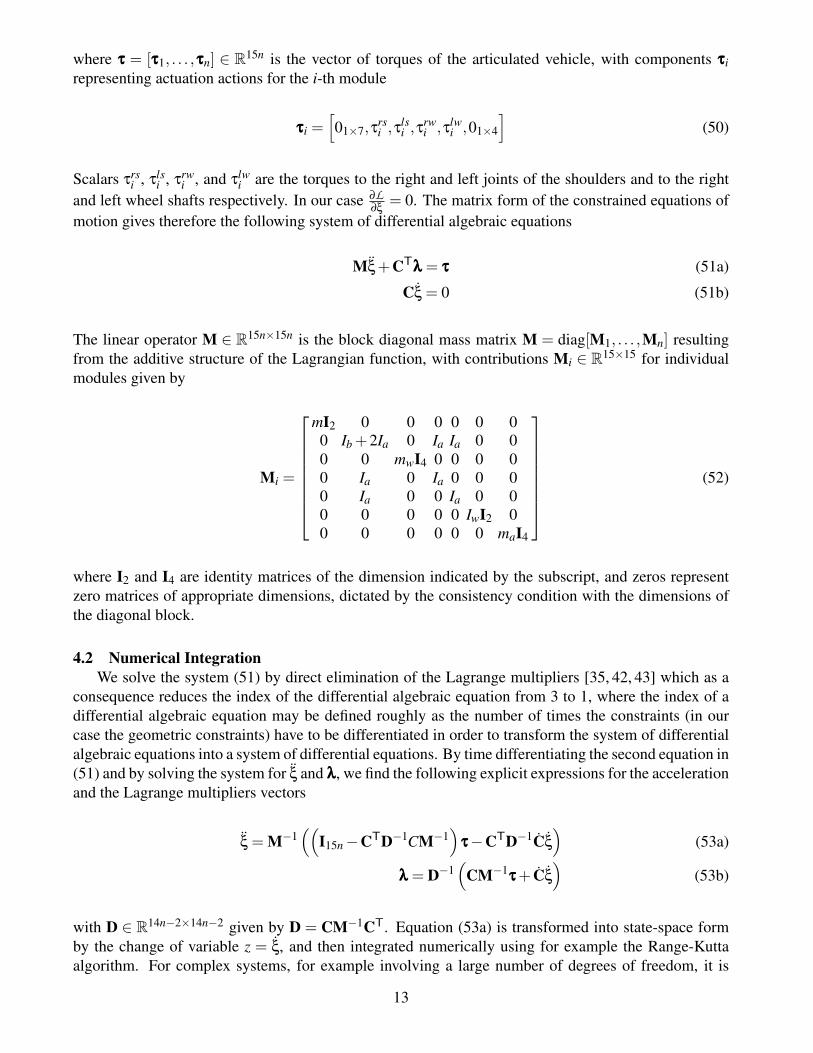
where τττ = [τττ1, . . . ,τττn] ∈ R15n is the vector of torques of the articulated vehicle, with components τττirepresenting actuation actions for the i-th module

τττi =[01×7,τ

rsi ,τ

lsi ,τ

rwi ,τlw

i ,01×4

](50)

Scalars τrsi , τls

i , τrwi , and τlw

i are the torques to the right and left joints of the shoulders and to the rightand left wheel shafts respectively. In our case ∂L

∂ξ= 0. The matrix form of the constrained equations of

motion gives therefore the following system of differential algebraic equations

Mξ+CTλλλ = τττ (51a)

Cξ = 0 (51b)

The linear operator M ∈ R15n×15n is the block diagonal mass matrix M = diag[M1, . . . ,Mn] resultingfrom the additive structure of the Lagrangian function, with contributions Mi ∈ R15×15 for individualmodules given by

Mi =

mI2 0 0 0 0 0 00 Ib +2Ia 0 Ia Ia 0 00 0 mwI4 0 0 0 00 Ia 0 Ia 0 0 00 Ia 0 0 Ia 0 00 0 0 0 0 IwI2 00 0 0 0 0 0 maI4

(52)

where I2 and I4 are identity matrices of the dimension indicated by the subscript, and zeros representzero matrices of appropriate dimensions, dictated by the consistency condition with the dimensions ofthe diagonal block.

4.2 Numerical IntegrationWe solve the system (51) by direct elimination of the Lagrange multipliers [35, 42, 43] which as a

consequence reduces the index of the differential algebraic equation from 3 to 1, where the index of adifferential algebraic equation may be defined roughly as the number of times the constraints (in ourcase the geometric constraints) have to be differentiated in order to transform the system of differentialalgebraic equations into a system of differential equations. By time differentiating the second equation in(51) and by solving the system for ξ and λλλ, we find the following explicit expressions for the accelerationand the Lagrange multipliers vectors

ξ = M−1((

I15n−CTD−1CM−1)

τττ−CTD−1Cξ

)(53a)

λλλ = D−1(

CM−1τττ+ Cξ

)(53b)

with D ∈ R14n−2×14n−2 given by D = CM−1CT. Equation (53a) is transformed into state-space formby the change of variable z = ξ, and then integrated numerically using for example the Range-Kuttaalgorithm. For complex systems, for example involving a large number of degrees of freedom, it is

13

appropriate to use advanced O(N) or O(logN) algorithms [44–46]. This method has the drawback tobe potentially unstable if the numerical integration is extended over a relatively long time interval, sincethe constraints are enforced at the acceleration level and therefore errors can accumulate for the velocityand position. Therefore, the constraints on position and velocity must be enforced explicitly in order toavoid the drift phenomena associated to the propagation of truncation and round-off errors. For a similarapproach the reader can refer to [43, 47].

5 Motion Control Inside a Pipe: a Show CaseHere we present an application of the model presented in previous sections. The objective of this

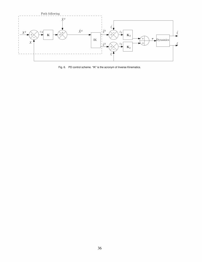
study is to illustrate it through simulations that involve some peculiarity of the scenarios for which oursystem will be designed and implemented. The environment is a planar strip that models the longitudinalsection of a pipeline in which the robot is deployed. We consider a path following kinematic control totrack the axis of the pipeline to reproduce the optimal operational condition of several sensors mountedon inspection mobile robots. The path planner is coupled with a PD torque control based on the dynamicmodel, that estimates the torques (actuators efforts) necessary to track the desired trajectory. The controlscheme is sketched in Fig. 6.

5.1 Path Following using Frenet FramesAs stated in the Introduction, the main targeted application of the system is pipeline maintenance

and inspection. Several sensing devices used for this class of applications have maximum performancewhen centered on the axis of the pipe. In order to simulate this scenario a path following controlstrategy which consists of tracking the center line of the pipe with the head (first module with respectto the forward motion) of the articulated robot is considered. The path following control defines thedesired kinematics, and it is coupled to a torque control to generate the torques necessary to track suchdesired kinematics.

The articulated mobile robot formed with n modules presents n+2 degrees of freedom, see Section2. Here we choose to control the pose of the head of the articulated vehicle, described by the vector(xG1,yG1,θ1), along with the orientations θ2, . . . ,θn of the other modules. Therefore the feedback loopin the path following control generates as many inputs (n+ 2) as the dimension of a minimal set ofcoordinates that describes the state of the articulated robot. The current choice implies that the centerof mass of the modules other than the head do not necessarily track the axis of the pipeline, whereas thelocal orientation of the path is tracked. Different choices are possible to achieve different objectives, asfor example tracking the path with the center of mass of each module, which require the control inputsto depend on the local distances between the centers of mass and the path.

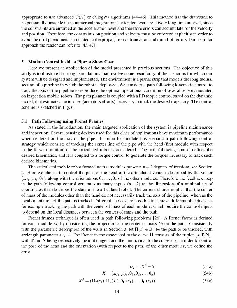
Frenet frames technique is often used in path following problems [26]. A Frenet frame is definedfor each module Mi by considering the projection of the center of mass Gi on the path. Consistentlywith the parametric description of the walls in Section 3, let ΠΠΠ(s) ∈ R2 be the path to be tracked, witharclength parameter s ∈ R. The Frenet frame associated to the curve ΠΠΠ consists of the triplet s,T,N,with T and N being respectively the unit tangent and the unit normal to the curve at s. In order to controlthe pose of the head and the orientation (with respect to the path) of the other modules, we define theerror

εX := Xd−X (54a)X = (xG1,yG1 ,θ1,θ2, . . . ,θn) (54b)

Xd = (Πx(s1),Πy(s1),θΠΠΠ(s1), . . .θΠΠΠ(sn)) (54c)

14

where Πx and Πy are the global Cartesian components of the point ΠΠΠ, si is the arclength associated to theprojection of Gi on the path, and θΠΠΠ is the global orientation of the tangent T, defined by tanθΠΠΠ = Ty/Tx.Therefore X is a minimal set of coordinates, and Xd (that depends on the path) is the correspondingcollection of desired states for X . In order to asymptotically drive the head of the robot to the path andto track the orientation of the path with the other modules, we define the variable Xd with first orderevolution described by

˙Xd = KεX + Xd (55)

where K = diag[Kx,Ky,Kθ1 , . . . ,Kθn] ∈ Rn+2×n+2 is a positive definite gain matrix. The state Xd can beinterpreted as the desired kinematics dictated by the path follower, that is mapped to the desired state ξd

through the inverse kinematics. Since cosθΠΠΠ(s1),sinθΠΠΠ(s1) are the components of the tangent vectorT(s1), we have

Xd =V (cosθΠΠΠ(s1),sinθΠΠΠ(s1),κΠΠΠ(s1), . . . ,κΠΠΠ(sn)) (56)

with the identifications si = V (forward speed) and ∂θΠΠΠ/∂si = κΠΠΠ (curvature), consistently with therelation

θΠΠΠ(si) = si∂θΠΠΠ

∂si(57)

Therefore if the error εX is zero, the desired kinematics corresponds to a forward motion with constantspeed V , with the head’s center of mass on the path, and with the modules oriented parallel to the localtangent (nearest point) of the path.

5.2 Torque ControlAs sketched in Fig. 6, we control the robot in the Cartesian space which involves the use of in-

verse geometric and inverse kinematic models. The desired kinematics ξd, ˙ξd is provided by the path

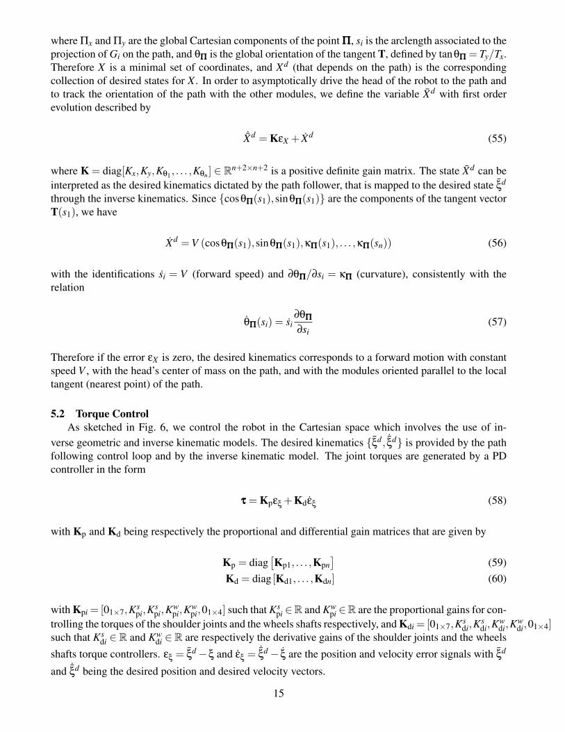
following control loop and by the inverse kinematic model. The joint torques are generated by a PDcontroller in the form

τττ = Kpεξ +Kdεξ (58)

with Kp and Kd being respectively the proportional and differential gain matrices that are given by

Kp = diag[Kp1, . . . ,Kpn

](59)

Kd = diag [Kd1, . . . ,Kdn] (60)

with Kpi = [01×7,Kspi,K

spi,K

wpi,K

wpi,01×4] such that Ks

pi ∈R and Kwpi ∈R are the proportional gains for con-

trolling the torques of the shoulder joints and the wheels shafts respectively, and Kdi = [01×7,Ksdi,K

sdi,K

wdi,K

wdi,01×4]

such that Ksdi ∈R and Kw

di ∈R are respectively the derivative gains of the shoulder joints and the wheelsshafts torque controllers. εξ = ξd−ξ and εξ =

˙ξd− ξ are the position and velocity error signals with ξd

and ˙ξd being the desired position and desired velocity vectors.

15

The PD controller tracks a time invariant desired kinematics with zero steady-state error. In order toprove it, we first transform the system of equations (51) by introducing the matrix P ∈ Rn+2×15n whoserows are n+ 2 linearly independent vectors in the null space of C. We define the reduced velocityη ∈ Rn+2 by

ξ = PTη (61)

Substitution into equation (51b) gives

CPTη = 0 (62)

which holds for all η ∈ Rn+2. Substitution into equation (51a), and pre-multiplication by P gives thereduced system

M?(η)η+W(η,η)η = τττ?(η) (63)

by accounting for the relation PC = 0. Additional symbols in (63) are given by Rn+2×n+2 3M?(η) =PMPT, Rn+2×n+2 3W(η,η) = PMPT, and Rn+2(η) 3 τττ? = Pτττ.

A time invariant path as described in the previous section is defined by constant θΠΠΠ. Indeed in thiscase the desired path kinematics is defined by a constant set provided that the forward speed is constant.By adapting a well known result, see for example [40, Chapter 8], we can prove that the system (53a)asymptotically tracks n + 2 time invariant desired parameters. To do so we consider the Lyapunovfunction

V =12

ηTM?

η+12

εTξ

Kpεξ (64)

Time deriving we obtain

V = ηTM?

η+12

ηTM?

η+ εTξ

Kpεξ (65)

For a time invariant desired trajectory, that is ξd = 0, substitution from (63) and (61) gives

V =12

ηT(M?−2W

)η+ η

Tτττ?− η

TPKpεξ (66)

By adopting the linear feedback τττ? = Pτττ = PKpεξ +PKdεξ with time invariant desired trajectory, andby the fact that the matrix M?−2W is skew-symmetric since

M?−2W = PMPT−PMPT (67)

the time derivative of the Lyapunov function simplifies to

V =−ηTK?

dη≤ 0 (68)

16

where K?d = PKdPT, and the equality holds for η = 0. Therefore V decreases along the trajectories for

nonzero η. In order to complete the proof we need to show that the largest invariant set is εξ = 0. To doso, assume that V ≡ 0 (which means that V is identically equal to zero). Then (68) implies η≡ 0 andtherefore η≡ 0. The equation of motion (22) with linear feedback then implies Kpεξ = 0. Let

δ := (δ1, . . . ,δn) (69)

with

δi :=(

αri ,α

li,θ

ri ,θ

li

)(70)

be the collection of actuated states, corresponding to nonzero entries of the diagonal gain matrix Kp.Consider the map

ϕϕϕ : Rn+2 3 η 7→ ϕϕϕ(η) = δ ∈ R4n (71)

By indicating with Kp the diagonal matrix obtained from Kp by extracting the nonzero elements, wehave

Kpεξ = Kpεδ (72)

where εδ = δ−δd , with δd being the desired state for δ. Since Kp is full rank

Kpεδ = 0⇒ εδ = 0 (73)

By LaSalle’s theorem [48, Chapter 5] the equilibrium is globally asymptotically stable, and thereforeδ→ δd . In terms of the minimal set η this implies that ϕϕϕ(η)→ ϕϕϕ(ηd). If the map ϕϕϕ is one to one, thenεη = ηd−η is globally asymptotically stable.

Moreover, if the map ϕϕϕ is non-singular in a neighborhood of the desired state ηd , it is well definedthe linearization

δ = δd +ΦΦΦ(η−η

d) (74)

where δd = ϕϕϕ(ηd), and ΦΦΦ = ∇ηϕϕϕ(ηd) ∈R4n×n+2 is the gradient of ϕϕϕ at ηd . In this case the equilibriumεη is locally asymptotically stable since εδ = 0⇒ΦΦΦεη = 0.

Note that for n > 0 the number of actuated states (4n) always exceeds the number of degrees offreedom of the articulated robot (n+ 2), and therefore the mechanism is redundantly actuated. Basedon the discussion above, it is clear that if the Jacobian C is full rank the actuated states collected in δ

asymptotically track the corresponding desired ones. On the neighborhood of a non-singular desiredminimal configuration ηd , the inverse relation between η and δ can be expressed as

η = ηd +ΦΦΦ

†εδ +(In+2−ΦΦΦ

†ΦΦΦ)η (75)

17

where ΦΦΦ† = ΦΦΦ

T(

ΦΦΦΦΦΦT)−1∈ Rn+2×4n is the right Moore-Penrose pseudoinverse of ΦΦΦ, and (In+2−

ΦΦΦ†ΦΦΦ)η is a vector in the null space of ΦΦΦ for every η ∈ Rn+2. The redundancy allows to exploit the

arbitrariness of η to achieve different desired states for η for the same εδ (eventually zero, as in ourcase). However, here we consider the minimum least square solution of the inverse kinematics and setη = 0.

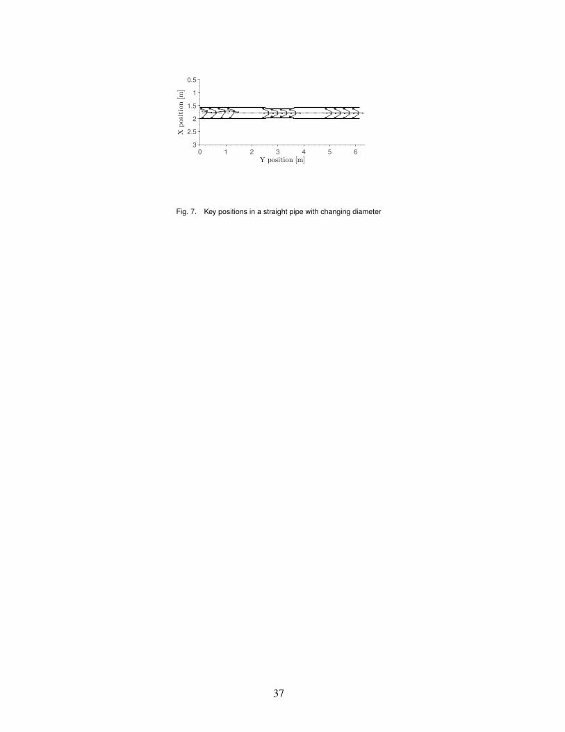
5.2.1 Crossing a Pipe with Changing DiameterThe objective of this simulation is to illustrate the model of the multibody mechanism by showing

the performance of the control strategy in following the center line of the pipe. In addition, it shows howthe structure adapts to changes in the pipe diameter (a restriction followed by an enlargement). The firstpart of the pipe is 2.5m long with diameter 42cm followed by a 1m length pipe with diameter of 34cmand a final portion 2.5m long with diameter of 42cm. The geometry of each module is determined bythe set of parameters h = 35cm (height), W = 10cm (width), ρ = 3cm (wheels radius), L = 24cm (armlength), and γ = 0.5. The kinematic path following is defined by the the gains Kx = Ky = 3 and Kθ = 3.The discrete time simulation scheme is run with sampling time 0.025 s. The gains for the torque controlare Ks

pi = 0.7, Ksdi = 0.2, and Kw

di = 0.03 for i = 1, . . . ,n. The proportional part of the wheel torquecontrol is set to zero since the angular position of the wheel shaft is unbounded.

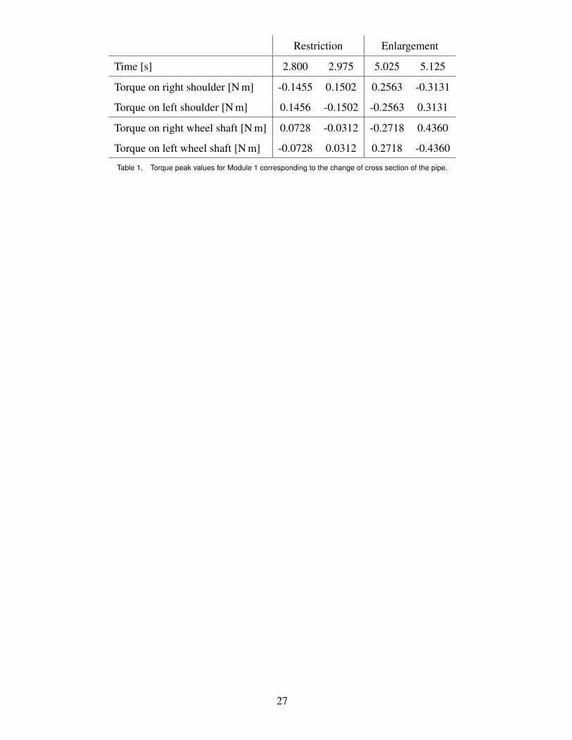
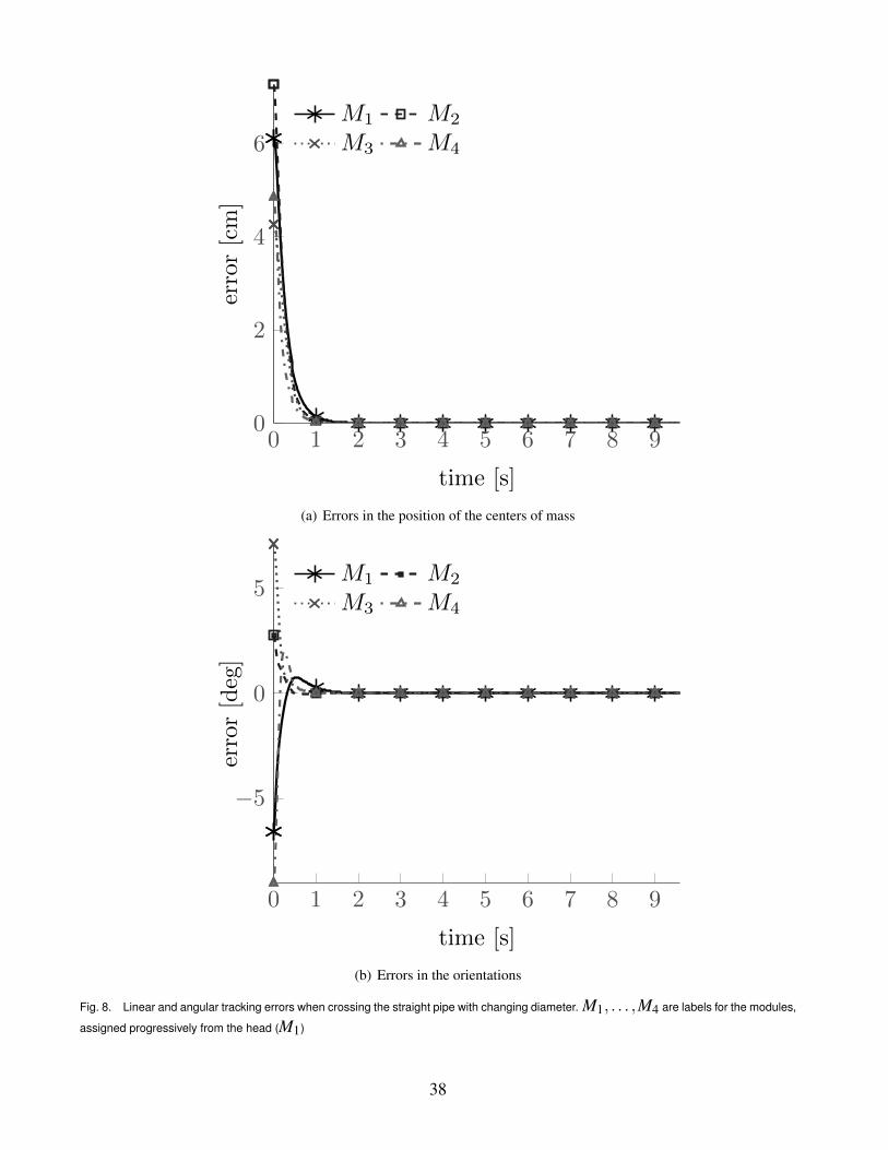
Figure 7 depicts a snapshot of three positions of the vehicle inside the pipe: initial, mid-length andfinal. The distance and orientation errors are stabilized asymptotically as shown in Figure 8, and asqualitatively confirmed by the inspection of Figure 7. Since the system is centered on the axis of thepipeline by the time the first module reaches the restriction, the torques generated by the controller toreact to the restriction are of equal magnitude and opposite sign, as shown in Table 1 for the head of therobot. Tables reporting results for the other modules are given in the Appendix. Due to this symmetry,the net action on the module due to the restriction is zero and therefore there is no perturbation. Sameconsiderations hold for the enlargement of the pipe.

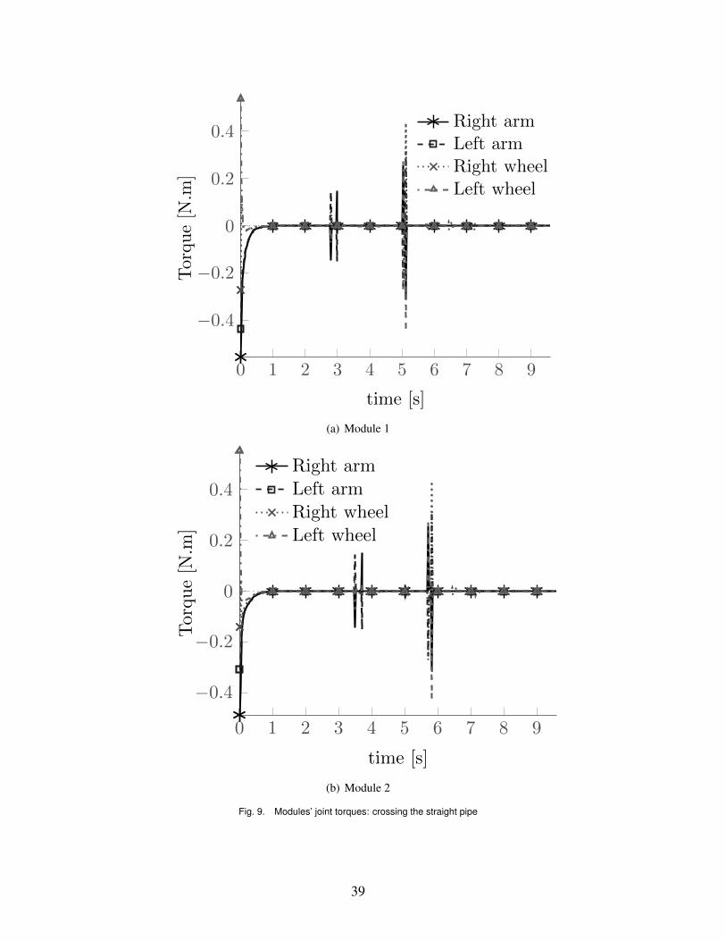
For the first two modules, the joint torques corresponding to this simulation are displayed on Fig-ure 9. For all the modules, the torque curves exhibit a similar shape, that is flat with two peak areasthat propagate among the modules. These peaks are the joints reaction to the two successive changesin pipe diameter. Since the articulated mechanism is centered on the axis by the time the first modulereaches the restriction, the torques generated are the same for each module with a characteristic timeshift that depends on the distance among wheels belonging to contiguous modules, and on the updatingtime step. If we consider the restriction as an obstacle, as the wheels meet the pipe restriction theydecelerate while the arms are closing. When they leave the restriction and enter the enlargement, thewheels accelerate while the arms spread. Note that the right wheel angular velocity is anti-clockwisewhen a module moves in the direction of increasing arc length, which means that a negative value intorque for the right wheel shaft corresponds to an acceleration in the module’s direction of motion. Thiscoordinated motion is due to the enforcement of the internal constraints (closed kinematic chain) andexternal constraints (permanent contact of the wheels with the pipe) while the module tracks the centerline with a constant velocity. The rest of the time the torques are almost zero due to the fact that the pipeportions in which the vehicle is travelling are straight. However, one can notice slight disturbances inthe wheel shaft torque curves of every module due to the manoeuvres of other modules each time theycross the restriction.

5.2.2 Crossing a Pipe with an ElbowHere, we show the operation of the robot while crossing two straight pipe sections connected by

a 3π/4 elbow. The diameter of the pipe is constant but the pipe presents a change in curvature. Wefollow a path with piecewise constant curvature. A constant curvature allows for the forward and lateral

18

motions to be decoupled, so that the path following problem can be treated as the problem of determiningthe asymptotic stability of the lateral motion [49], with the system driven by the longitudinal motion.Numerical values for the gains of the path following controller and for the torque controller are thesame as the ones listed above for the case of straight pipe with restriction, and the sampling time forthe discrete time integration algorithm is 0.02 s for simulations involving one module, and 0.025 s forsimulations involving the articulated vehicle.

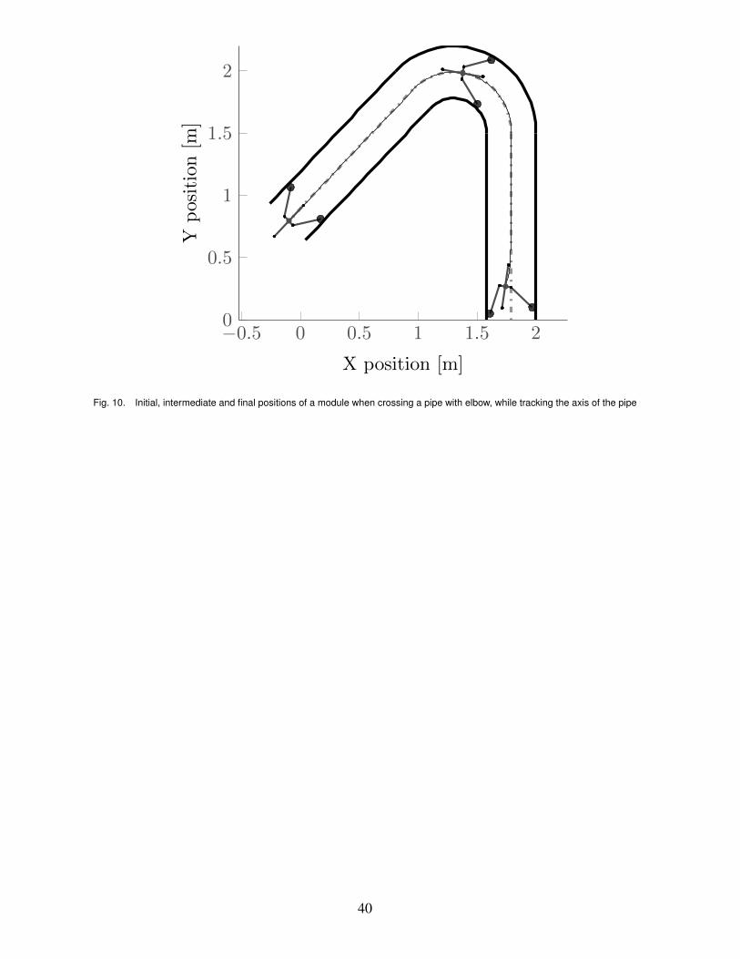
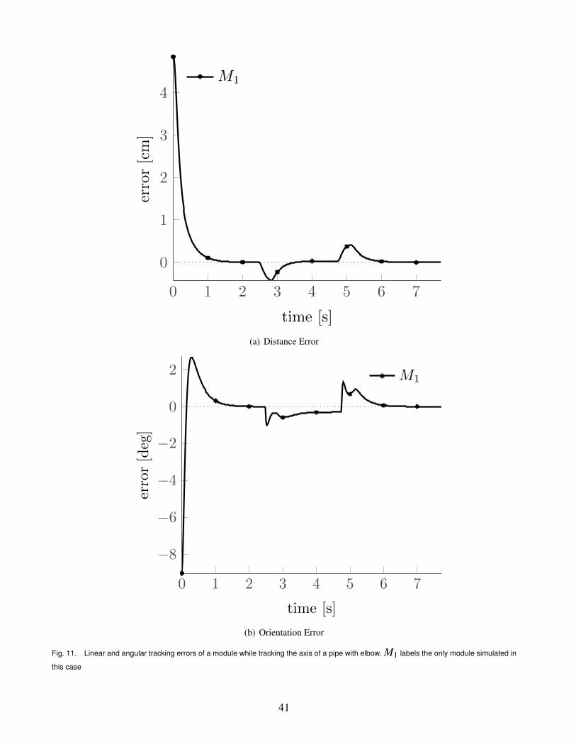
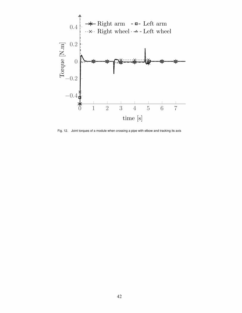
For a single module, Figure 10 illustrates three key positions while crossing the pipe with elbow.The distance and orientation errors for this simulation depicted on Figure 11 converge to zero with twosaddle points that are due to the two successive changes in curvature when the module enters and leavesthe elbow. This emerges also on the curves depicted on Figure 12, showing the reaction of the joints interms of torque in response to the curvature changes.

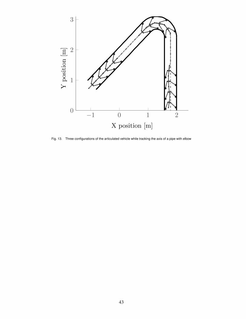
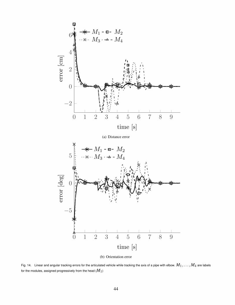
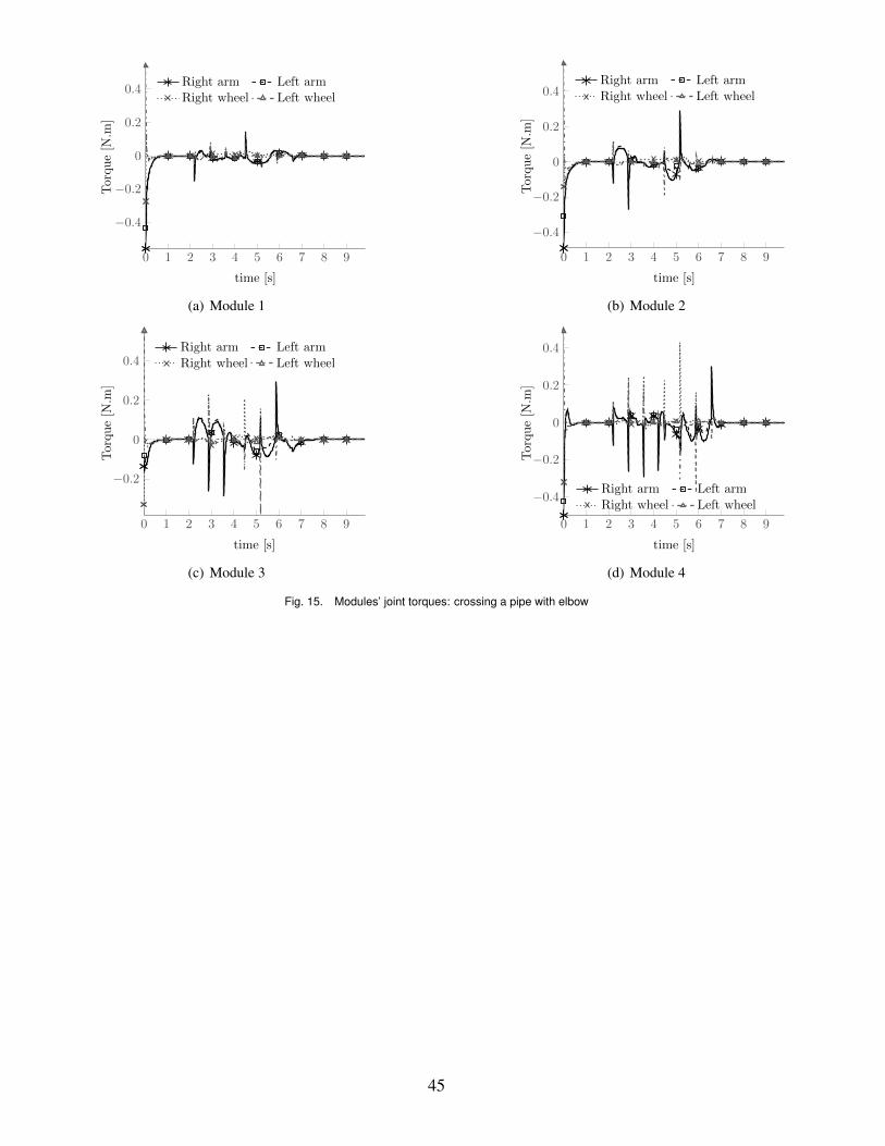
For the case of the articulated vehicle, we apply the same control scheme as for the pipe withrestriction, with the same numerical values of the geometric and control parameters. Figure 13 shows asnapshot of the articulated vehicle inside the pipe with elbow. Distance and orientation error curves areshown on Figures 14. Since the head pose is fully controlled its distance and orientation errors exhibitthe expected better result, especially in the distance error, as compared to the the rest of modules forwhich only the orientations are controlled. The torques applied by the joints are shown in Figure 15 forthe four modules. Notice the difference in the efforts produced by the joints of the modules as part ofthe articulated vehicle when compared to the case of a module evolving separately (Figure 12). Everymodule is subjected to inner structural constraints and also to hitching constraints. In the case of achange of curvature, the interactions between the modules forming the articulated vehicle are importantand visible compared to the case of crossing a straight pipe with changing diameter. This shows that achange of curvature introduces a challenging scenario as the proportional controller cannot compensatefor the disturbance introduced by it, as opposed to the case of change of diameter of the cross section.

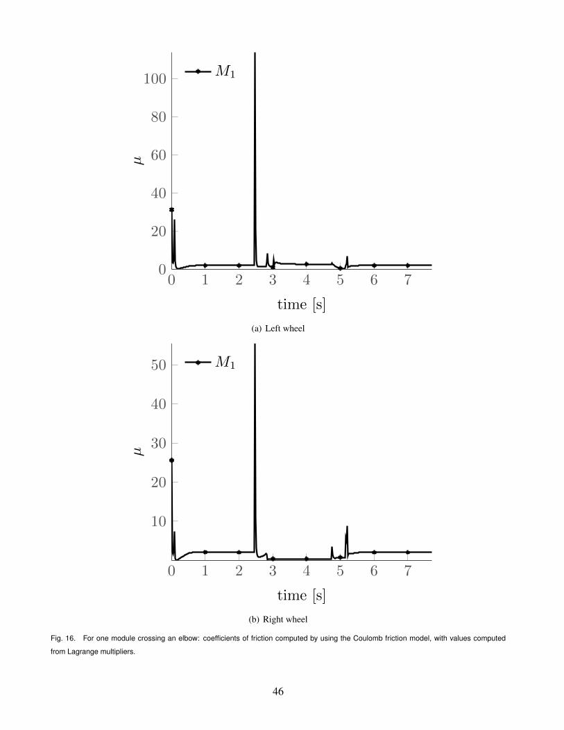
The rolling without slipping constraint adopted here is enforced by virtue of a set of Lagrange multi-pliers that quantify the contact forces (Cartesian components) required to guarantee that such constraintis not violated. This does not imply that the contact forces are physically admissible, as for examplethe friction required to enforce the no slip condition could be too high for the materials involved. Theassessment of the physical compatibility would require the introduction of a specific set of constitutiverelations that relate the contact forces to the kinematic duals (tangential velocities), as it is done forexample in [13]. However, within the model considered in this work, the contact forces involved in theevolution of the robot when the rolling without slipping constraints hold, are computed directly throughequation (53b), and they can be used to estimate the material properties (coefficients of friction) neces-sary to guarantee the non violation of the constraint, or eventually the non compatibility with commonlyused materials. To illustrate this we show in Figure 16 the coefficients of friction, obtained through asimple Coulomb friction model, as the ratio

µ =FT

FN(76)

between the tangential and the normal components, FT and FN respectively, of the contact forces be-tween walls and wheels. Results refer to the example of one module crossing an elbow, and the tangen-tial and normal components are obtained from the Cartesian components λx and λy by solving the linearsystem

λx = FT Tx +FNNx (77a)λy = FT Ty +FNNy (77b)

19

where Tx, Ty, Nx, and Ny are the Cartesian components of the tangent and of the normal vector fields.The coefficients of friction in Figure 16 are shown for the right and for the left wheels, and therefore

two sets of Lagrange multipliers are involved, with corresponding two Frenet frames (and unit vectors)associated to the two walls. Peaks of the values of the estimated coefficients of friction may correspondto non-realizable scenarios in terms of materials, as typically the coefficients of friction for commonengineering pairs of materials range between 0.1 to 1.5.

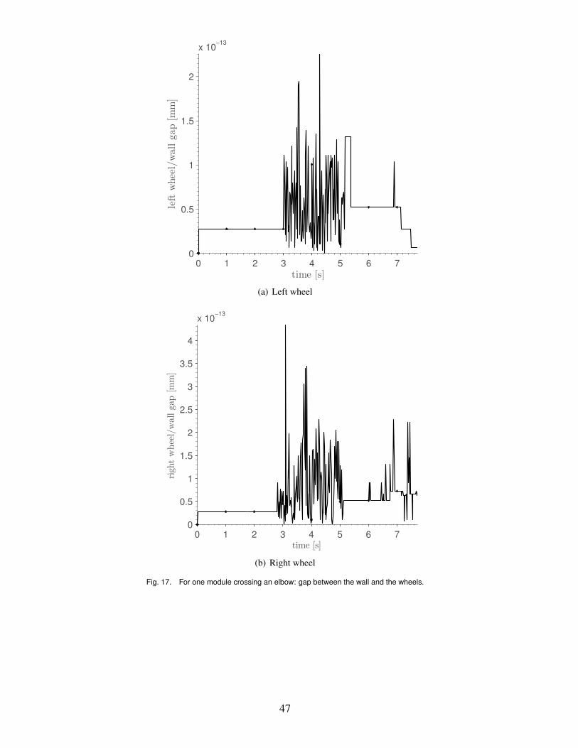
The gap between the wheels nearest points to the wall and the corresponding point on the wall,plotted in Figure 17, shows that the rolling without slipping constraints are correctly enforced duringthe simulation.

6 ConclusionsIn this paper, we derived the dynamics of an articulated mobile robot tailored for the exploration

of confined environments, more specifically for in-pipe inspection applications. The kinematics of therobot is described by a chain of parallel mechanisms on mobile platforms. This kinematics is charac-terized by a larger number of degrees of freedom, and therefore available control inputs, with respectto other articulated vehicles such as the n-trailer. The augmented number of degrees of freedom corre-sponds to more versatility in executing some pipe inspections maneuvers such as turning sharp angleswhile maintaining the robot axially centered to maximize sensor performance.

The model derivation is based on Lagrange’s formulation for constrained multibody dynamics. Wefirst derived the equations of motion of one module that we extended to the whole articulated vehicle.The model is illustrated through simulations of motion inside a pipe. A path following controller isused together with a torque controller for the navigation of the vehicle to track the center line of a pipefor two different operational scenarios: a straight pipe with changing diameter and a pipe with 3π/4elbow. Simulation results illustrate the effectiveness of the dynamic model in predicting the actuationefforts involved in the two considered operational scenarios, that can be typically encountered whenthere is an obstruction of the cross section of the pipe, and when the robot has to negotiate a change ofdirection. The model allows to simulate critical situations and to predict the actions necessary to track adesired trajectory for sensor performance maximization. It is therefore possible to design control gainsthat minimize the energy consumption associated to control actions, and ultimately to maximize theautonomy of the robot.

The design of advanced control laws to improve the coordination of the modules and to handle themore general case of paths with varying curvatures is part of ongoing works. The model of the threedimensional version of the robot is also part of future work.

AcknowledgementsThis work was partially funded by the Federal Economic Development Agency for Southern Ontario

through the SME4SME program, and partially by NSERC through the Discovery program.A special acknowledgement to InvoDane Engineering, Ltd. for the collaboration through the grant

SME4SME.

20

References[1] Hirose, S., and Morishima, A., 1990. “Design and control of a mobile robot with an articulated

body”. Journal of Robotics Research, 9(2), pp. 99–114.[2] Mirats Tur, J., and Garthwaite, W., 2010. “Robotic devices for water main in-pipe inspection: A

survey”. Journal of Field Robotics, 27(4), pp. 491–508.[3] Mazumdar, A., and Asada, H. H., 2010. “An Underactuated, Magnetic-Foot Robot for Steel

Bridge Inspection”. Journal of Mechanics and Robotics-Transactions of the ASME, 2(3), Aug,pp. 031007–031007–9.

[4] Suzumori, K., Wakimoto, S., and Takata, M., 2003. “A miniature inspection robot negotiatingpipes of widely varying diameter”. In 2003 IEEE International Conference on Robotics and Au-tomation, VOLS 1-3, Proceedings, pp. 2735–2740.

[5] Schempf, H., Mutschler, E., Goltsberg, V., Skoptsov, G., Gavaert, A., and Vradis, G., 2003. “Ex-plorer: Untethered real-time gas main assessment robot system”. In Proc. of Int. Workshop onAdvances in Service Robotics, ASER’03.

[6] Jamoussi, A., 2005. “Robotic NDE: A new solution for in-line pipe inspection”. In Middle EastNondestructive Testing Conference and Exhibition.

[7] Fjerdingen, S. A., Liljeback, P., and Transeth, A. A., 2009. “A snake-like robot for internal inspec-tion of complex pipe structures (PIKo)”. In 2009 IEEE/RSJ International Conference on IntelligentRobots and Systems, pp. 5665–5671.

[8] Shin, H., Jeong, K.-M., and Kwon, J.-J., 2010. “Development of a Snake Robot Moving in a SmallDiameter Pipe”. In International Conference on Control, Automation and Systems (ICCAS 2010),pp. 1826–1829.

[9] Dertien, E., Stramigioli, S., and Pulles, K., 2011. “Development of an inspection robot for smalldiameter gas distribution mains”. In Robotics and Automation (ICRA), 2011 IEEE InternationalConference on, pp. 5044–5049.

[10] Transeth, A. A., and Pettersen, K. Y., 2006. “Developments in snake robot modeling and loco-motion”. In International Conference on Control, Automation, Robotics and Vision ICARCV,pp. 1–8.

[11] Wiriyacharoensunthorn, P., and Laowattana, S., 2002. “Analysis and design of a multi-link mobilerobot (serpentine)”. In IEEE International Conference on Industrial Technology, Vol. 2, pp. 694–699.

[12] Ostrowski, J., and Burdick, J., 1996. “Gait kinematics for a serpentine robot”. In Proceedings ofthe IEEE International Conference on Robotics and Automation, Vol. 2, pp. 1294–1299.

[13] Transeth, A. A., Leine, R. I., Glocker, C., Pettersen, K. Y., and Liljeback, P., 2008. “Snakerobot obstacle-aided locomotion: modeling, simulations, and experiments”. IEEE Transactionson Robotics, 24(1), pp. 88–104.

[14] Ma, S., and Tadokoro, N., 2006. “Analysis of creeping locomotion of a snake-like robot on aslope”. Autonomous Robots, 20(1), pp. 15–23.

[15] Bayraktaroglu, Z. Y., and Blazevic, P., 2005. “Understanding snakelike locomotion through a novelpush-point approach”. Journal of dynamic systems, measurement, and control, 127(1), pp. 146–152.

[16] Hopkins, J. K., Spranklin, B. W., and Gupta, S. K., 2011. “A Case Study in Optimization ofGait and Physical Parameters for a Snake-Inspired Robot Based on a Rectilinear Gait”. Journal ofMechanics and Robotics-Transactions of the ASME, 3(1), Feb.

[17] Briot, S., Glazunov, V., and Arakelian, V., 2013. “Investigation on the Effort Transmission inPlanar Parallel Manipulators”. Journal of Mechanics and Robotics-Transactions of the ASME,5(1), Feb.

[18] Carretero, J. A., Ebrahimi, I., and Boudreau, R., 2012. “Overall Motion Planning for Kinematically

21

Redundant Parallel Manipulators”. Journal of Mechanics and Robotics-Transactions of the ASME,4(2), May.

[19] Hu, B., Yu, J., Lu, Y., Sui, C., and Han, J., 2012. “Statics and Stiffness Model of Serial-ParallelManipulator Formed by k Parallel Manipulators Connected in Series”. Journal of Mechanics andRobotics-Transactions of the ASME, 4(2), May.

[20] Bolzern, P., DeSantis, R., Locatelli, A., and Togno, S., 1996. “Dynamic model of a two-trailerarticulated vehicle subject to nonholonomic constraints”. Robotica, 14(4), pp. 445–450.

[21] Ute, J., and Ono, K., 2002. “Fast and efficient locomotion of a snake robot based on self-excitationprinciple”. In 7TH International Workshop on Advanced Motion Control, Proceedings, pp. 532–539.

[22] Transeth, A. A., Leine, R. I., Glocker, C., and Pettersen, K. Y., 2008. “3-D snake robot motion:Nonsmooth modeling, simulations, and experiments”. IEEE Transactions on Robotics, 24(2),pp. 361–376.

[23] Transeth, A. A., Leine, R. I., Glocker, C., Pettersen, K. Y., and Liljeback, P., 2008. “Snakerobot obstacle-aided locomotion: Modeling, simulations, and experiments”. IEEE Transactionson Robotics, 24(1), pp. 88–104.

[24] Liljeback, P., Pettersen, K. Y., Stavdahl, O., and Gravdahl, J. T., 2010. “A simplified model ofplanar snake robot locomotion”. In IEEE/RSJ 2010 International Conference on Intelligent Robotsand Systems (IROS 2010), pp. 2868–2875.

[25] Liljeback, P., Pettersen, K., Stavdahl, O., and Gravdahl, J., 2010. “Hybrid modelling and controlof obstacle-aided snake robot locomotion”. IEEE Transactions on Robotics, 26(5), pp. 781–799.

[26] Murugendran, B., Transeth, A. A., and Fjerdingen, S. A., 2009. “Modeling and Path-following fora Snake Robot with Active Wheels”. In 2009 IEEE-RSJ International Conference on IntelligentRobots and Systems, pp. 3643–3650.

[27] Li, N., Zhao, T., and Zhao, Y., 2008. “The dynamic modeling of snake-like robot by using nominalmechanism method”. In ICIRA ’08 Proceedings of the First International Conference on IntelligentRobotics and Applications: Part I, pp. 1185–1194.

[28] Liljeback, P., Pettersen, K., Stavdahl, O., and Gravdahl, J., 2012. “A review on modelling, imple-mentation, and control of snake robots”. Robotics and Autonomous Systems, 60(1), pp. 29–40.

[29] Samin, J.-C., and Fisette, P., 2003. Symbolic Modeling of Multibody Systems. Kluwer AcademicPub.

[30] Bendtsen, C., and Thomsen, P., 1999. Numerical Solution of Differential Algebraic Equations.IMM, Department of Mathematical Modeling, Technical University of Denmark.

[31] Wijckmans, P., 1996. “Conditionning of differential algebraic equations and numerical solution ofmultibody dynamics”. PhD thesis, Technische Universiteit Eindhoven.

[32] Baumgarte, J., 1972. “Stabilization of constraints and integrals of motion in dynamical systems”.Computer Methods in Applied Mechanics and Engineering, 1(1), pp. 1–16.

[33] Cline, M. B., and Pai, D. K., 2003. “Post-stabilization for rigid body simulation with contact andconstraints”. In 2003 IEEE International Conference on Robotics and Automation, Proceedings,Vol. 1-3, pp. 3744–3751.

[34] Ascher, U., Chin, H., Petzold, L., and Reich, S., 1995. “Stabilization of constrained mechanicalsystems with DAEs and invariant manifolds”. Mechanics of Structures and Machines, 23, pp. 135–157.

[35] Bauchau, O., and Laulusa, A., 2008. “Review of contemporary approaches for constraint enforce-ment in multibody systems”. Journal of Computational and Nonlinear Dynamics, 3(1), pp. 1–8.

[36] Sarfraz, H., Spinello, D., Gueaieb, W., and Douadi, L., 2013. “Critical maneuvers of an au-tonomous parallel robot in a confined environment”. In Proceedings of the International Confer-ence of Mechanical Engineering and Mechatronics (ICMEM), pp. 196–1.

22

[37] Gosselin, C., and Angeles, J., 1990. “Singularity analysis of closed-loop kinematic chains”. IEEETransactions on Robotics and Automation, 6(3), pp. 281–290.

[38] Merlet, J. P., 2006. Parallel Robots. Springer.[39] Bernstein, D. S., 2011. Matrix Mathematics: Theory, Facts, and Formulas (Second Edition).

Princeton University Press.[40] Spong, M. W., Hutchinson, S., and Vidyasagar, M., 2006. Robot Modeling and Control. Wiley.[41] Flannery, M., 2004. “The enigma of nonholonomic constraints”. American Journal of Physics,

73(3), pp. 265–272.[42] Hemami, H., and Weimer, F. C., 1981. “Modeling of nonholonomic dynamic systems with appli-

cations”. Journal of Applied Mechanics, 48(1), pp. 177–182.[43] Metiku, R., 2004. “Computer-aided dynamic force analysis of four-bar planar mechanism.”. Mas-

ter’s thesis, Addis Ababa University. School of Graduate Studies.[44] Poursina, M., and Anderson, K. S., 2013. “An extended divide-and-conquer algorithm for a gen-

eralized class of multibody constraints”. Multibody System Dynamics, 29(3), pp. 235–254.[45] Kreutz-Delgado, K., Jain, A., and Rodriguez, G., 1991. “Recursive formulation of operational

space control”. In Robotics and Automation, 1991. Proceedings., 1991 IEEE International Con-ference on, pp. 1750–1753.

[46] Poursina, M., and Anderson, K. S., 2013. “Canonical ensemble simulation of biopolymers usinga coarse-grained articulated generalized divide-and-conquer scheme”. Computer Physics Commu-nications, 184(3), pp. 652–660.

[47] Yu, Q., and Chen, I.-M., 2000. “A direct violation correction method in numerical simulation ofconstrained multibody systems”. Computational Mechanics, 26(1), pp. 52–57.

[48] Sastry, S. S., 1999. Nonlinear Systems: Analysis, Stability, and Control. Springer.[49] Altafini, C., 2002. “Following a path of varying curvature as an output regulation problem”. IEEE

Transactions on Automatic Control, 47(9), pp. 1551–1556.

Appendix A: Complement to the section on kinematics

State dependent coefficients appearing on the closure kinematic equations (22)

ari =

12

W cosθi +Lsin(θi +αri )−H sinθi (78a)

cri =−Lsin(θi +α

ri ) (78b)

bri =

12

W sinθi−Lcos(θi +αri )+H cosθi (78c)

dri = Lcos(θi +α

ri ) (78d)

ali =−

12

W cosθi−Lsin(θi +αli)−H sinθi (78e)

cli = Lsin(θi +α

li) (78f)

bli =−

12

W sinθi +Lcos(θi +αli)+H cosθi (78g)

dli =−Lcos(θi +α

li) (78h)

23

Parallel and serial Jacobians in (32)

Jpi =

I2ar

ibr

i

I2al

ibl

i

04×2 04×1

04×2

L2 sin(θi +αr

i )−L

2 cos(θi +αri )

−L2 sin(θi +αl

i)L2 cos(θi +αl

i)

(79a)

Jqi =

I4

cri 0

dri 0

0 cli

0 dli

04×2 04×4

I4 04×2

ρNry(s

ri ) 0

−ρNrx(s

ri ) 0

0 −ρNly(s

li)

0 ρNlx(s

li)

04×4

I4

−L2 sin(θi +αr

i ) 0L2 cos(θi +αr

i ) 00 L

2 sin(θi +αli)

0 −L2 cos(θi +αl

i)

04×2 −I4

(79b)

Jacobians in (33)

Jp =

Jp1

Q1 S2Jp2

Q2 S3 0Jp3

Q3 S4. . .

0 Qn−1 Sn

Jpn

(80a)

Qi =

[1 0 Lb sinθi0 1 −Lb cosθi

]Si =

[−1 0 L f sinθi0 −1 −L f cosθi

](80b)

24

Jq =

Jq1

02×n

Jq2 002×n

0. . .

Jqn

(80c)

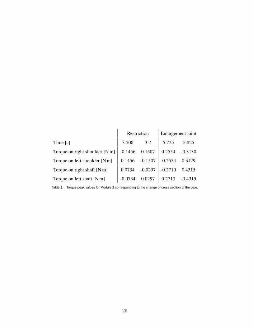
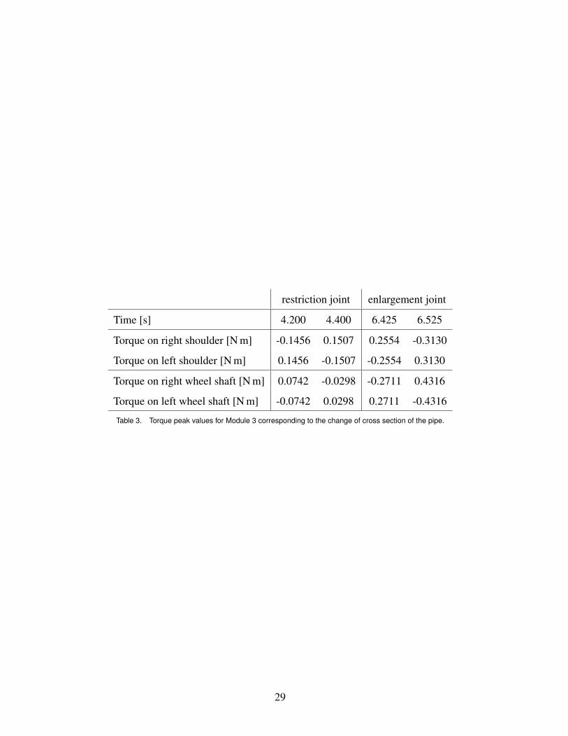
Appendix B: Additional Numerical Results in Section 5.2.1Torques generated by the controller to react to the changes of cross section of the pipeline: results

for Modules 2, 3, and 4 are shown respectively in Tables 2, 3, and 4.

25

List of Tables1 Torque peak values for Module 1 corresponding to the change of cross section of the pipe. 272 Torque peak values for Module 2 corresponding to the change of cross section of the pipe. 283 Torque peak values for Module 3 corresponding to the change of cross section of the pipe. 294 Torque peak values for Module 4 corresponding to the change of cross section of the pipe. 30

List of Figures1 Kinematic scheme of the articulated mobile robot. . . . . . . . . . . . . . . . . . . . . 312 Schematic of one module with notation. . . . . . . . . . . . . . . . . . . . . . . . . . 323 Right wheel contact with the pipe wall . . . . . . . . . . . . . . . . . . . . . . . . . . 334 Two serial singularities: (a) both arms are normal to the pipe walls, (b) only one arm is

normal to the wall . . . . . . . . . . . . . . . . . . . . . . . . . . . . . . . . . . . . . 345 Parallel singularity . . . . . . . . . . . . . . . . . . . . . . . . . . . . . . . . . . . . 356 PD control scheme. “IK” is the acronym of Inverse Kinematics. . . . . . . . . . . . . 367 Key positions in a straight pipe with changing diameter . . . . . . . . . . . . . . . . . 378 Linear and angular tracking errors when crossing the straight pipe with changing di-

ameter. M1, . . . ,M4 are labels for the modules, assigned progressively from the head(M1) . . . . . . . . . . . . . . . . . . . . . . . . . . . . . . . . . . . . . . . . . . . . 38

9 Modules’ joint torques: crossing the straight pipe . . . . . . . . . . . . . . . . . . . . 3910 Initial, intermediate and final positions of a module when crossing a pipe with elbow,

while tracking the axis of the pipe . . . . . . . . . . . . . . . . . . . . . . . . . . . . 4011 Linear and angular tracking errors of a module while tracking the axis of a pipe with

elbow. M1 labels the only module simulated in this case . . . . . . . . . . . . . . . . . 4112 Joint torques of a module when crossing a pipe with elbow and tracking its axis . . . . 4213 Three configurations of the articulated vehicle while tracking the axis of a pipe with elbow 4314 Linear and angular tracking errors for the articulated vehicle while tracking the axis of

a pipe with elbow. M1, . . . ,M4 are labels for the modules, assigned progressively fromthe head (M1) . . . . . . . . . . . . . . . . . . . . . . . . . . . . . . . . . . . . . . . 44

15 Modules’ joint torques: crossing a pipe with elbow . . . . . . . . . . . . . . . . . . . 4516 For one module crossing an elbow: coefficients of friction computed by using the

Coulomb friction model, with values computed from Lagrange multipliers. . . . . . . 4617 For one module crossing an elbow: gap between the wall and the wheels. . . . . . . . 47

26

Restriction Enlargement

Time [s] 2.800 2.975 5.025 5.125

Torque on right shoulder [N m] -0.1455 0.1502 0.2563 -0.3131

Torque on left shoulder [N m] 0.1456 -0.1502 -0.2563 0.3131

Torque on right wheel shaft [N m] 0.0728 -0.0312 -0.2718 0.4360

Torque on left wheel shaft [N m] -0.0728 0.0312 0.2718 -0.4360

Table 1. Torque peak values for Module 1 corresponding to the change of cross section of the pipe.

27

Restriction Enlargement joint

Time [s] 3.500 3.7 5.725 5.825

Torque on right shoulder [N m] -0.1456 0.1507 0.2554 -0.3130

Torque on left shoulder [N m] 0.1456 -0.1507 -0.2554 0.3129

Torque on right shaft [N m] 0.0734 -0.0297 -0.2710 0.4315

Torque on left shaft [N m] -0.0734 0.0297 0.2710 -0.4315

Table 2. Torque peak values for Module 2 corresponding to the change of cross section of the pipe.

28

restriction joint enlargement joint

Time [s] 4.200 4.400 6.425 6.525

Torque on right shoulder [N m] -0.1456 0.1507 0.2554 -0.3130

Torque on left shoulder [N m] 0.1456 -0.1507 -0.2554 0.3130

Torque on right wheel shaft [N m] 0.0742 -0.0298 -0.2711 0.4316

Torque on left wheel shaft [N m] -0.0742 0.0298 0.2711 -0.4316

Table 3. Torque peak values for Module 3 corresponding to the change of cross section of the pipe.

29

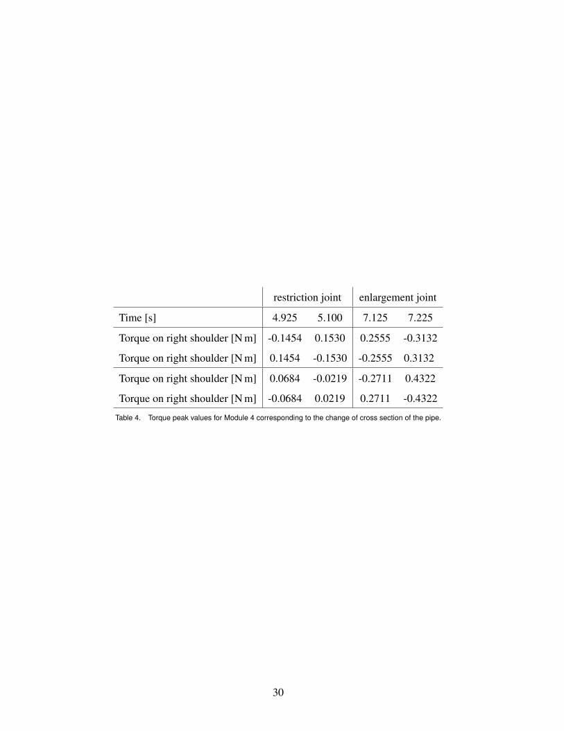
restriction joint enlargement joint

Time [s] 4.925 5.100 7.125 7.225

Torque on right shoulder [N m] -0.1454 0.1530 0.2555 -0.3132

Torque on right shoulder [N m] 0.1454 -0.1530 -0.2555 0.3132

Torque on right shoulder [N m] 0.0684 -0.0219 -0.2711 0.4322

Torque on right shoulder [N m] -0.0684 0.0219 0.2711 -0.4322

Table 4. Torque peak values for Module 4 corresponding to the change of cross section of the pipe.

30

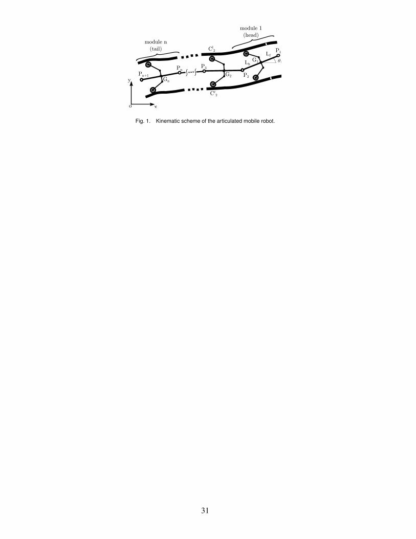
Fig. 1. Kinematic scheme of the articulated mobile robot.

31

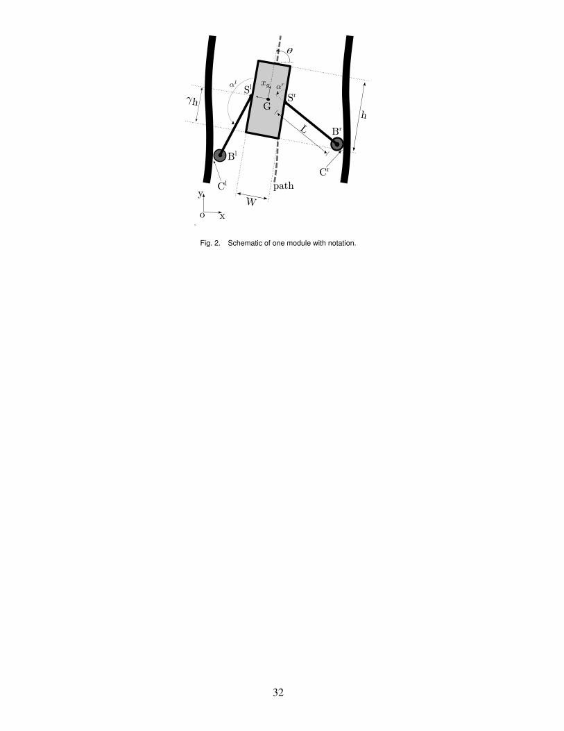
Fig. 2. Schematic of one module with notation.

32

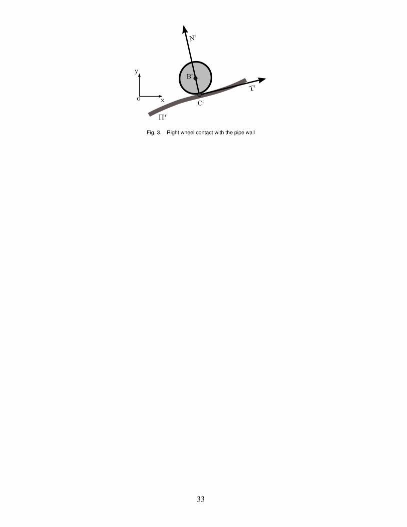
Fig. 3. Right wheel contact with the pipe wall

33

(a) (b)

Fig. 4. Two serial singularities: (a) both arms are normal to the pipe walls, (b) only one arm is normal to the wall

34

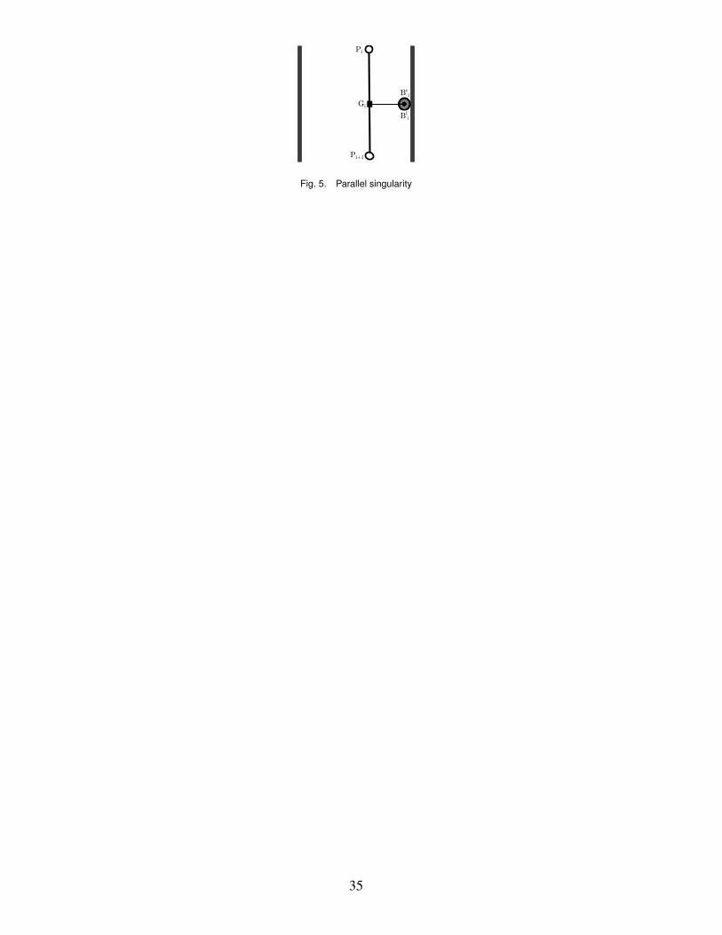
Fig. 5. Parallel singularity

35

+−

Xd

K ++εX

Xd

˙Xd

IK

ξd

˙ξd

+−

+−

Kd

εξ

Kp

εξ +

+ Dynamicsξ

ξ

τ

Path following

X

ξ

ξ

Fig. 6. PD control scheme. “IK” is the acronym of Inverse Kinematics.

36

0.5

1

1.5

2

2.5

3

0 1 2 3 4 5 6

Xposition[m

]

Y position [m]

Fig. 7. Key positions in a straight pipe with changing diameter

37

0 1 2 3 4 5 6 7 8 90

2

4

6

time [s]

error[cm]

M1 M2

M3 M4

(a) Errors in the position of the centers of mass

0 1 2 3 4 5 6 7 8 9

−5

0

5

time [s]

error[deg]

M1 M2

M3 M4

(b) Errors in the orientations

Fig. 8. Linear and angular tracking errors when crossing the straight pipe with changing diameter. M1, . . . ,M4 are labels for the modules,

assigned progressively from the head (M1)

38

0 1 2 3 4 5 6 7 8 9

−0.4

−0.2

0

0.2

0.4

time [s]

Torque[N

.m]

Right armLeft armRight wheelLeft wheel

(a) Module 1

0 1 2 3 4 5 6 7 8 9

−0.4

−0.2

0

0.2

0.4

time [s]

Torque[N

.m]

Right armLeft armRight wheelLeft wheel

(b) Module 2

Fig. 9. Modules’ joint torques: crossing the straight pipe

39

−0.5 0 0.5 1 1.5 20

0.5

1

1.5

2

X position [m]

Yposition[m

]

Fig. 10. Initial, intermediate and final positions of a module when crossing a pipe with elbow, while tracking the axis of the pipe

40

0 1 2 3 4 5 6 7

0

1

2

3

4

time [s]

error[cm]

M1

(a) Distance Error

0 1 2 3 4 5 6 7

−8

−6

−4

−2

0

2

time [s]

error[deg]

M1

(b) Orientation Error

Fig. 11. Linear and angular tracking errors of a module while tracking the axis of a pipe with elbow. M1 labels the only module simulated in

this case

41

0 1 2 3 4 5 6 7

−0.4

−0.2

0

0.2

0.4

time [s]

Torque[N

.m]

Right arm Left armRight wheel Left wheel

Fig. 12. Joint torques of a module when crossing a pipe with elbow and tracking its axis

42

−1 0 1 20

1

2

3

X position [m]

Yposition[m

]

Fig. 13. Three configurations of the articulated vehicle while tracking the axis of a pipe with elbow

43

0 1 2 3 4 5 6 7 8 9

−2

0

2

4

6

time [s]

error[cm]

M1 M2

M3 M4

(a) Distance error

0 1 2 3 4 5 6 7 8 9

−5

0

5

time [s]

error[deg]

M1 M2

M3 M4

(b) Orientation error

Fig. 14. Linear and angular tracking errors for the articulated vehicle while tracking the axis of a pipe with elbow. M1, . . . ,M4 are labels

for the modules, assigned progressively from the head (M1)

44

0 1 2 3 4 5 6 7 8 9

−0.4

−0.2

0

0.2

0.4

time [s]

Torque[N

.m]

Right arm Left armRight wheel Left wheel

(a) Module 1

0 1 2 3 4 5 6 7 8 9

−0.4

−0.2

0

0.2

0.4

time [s]

Torque[N

.m]

Right arm Left armRight wheel Left wheel

(b) Module 2

0 1 2 3 4 5 6 7 8 9

−0.2

0

0.2

0.4

time [s]

Torque[N

.m]

Right arm Left armRight wheel Left wheel

(c) Module 3

0 1 2 3 4 5 6 7 8 9

−0.4

−0.2

0

0.2

0.4

time [s]

Torque[N

.m]

Right arm Left armRight wheel Left wheel

(d) Module 4

Fig. 15. Modules’ joint torques: crossing a pipe with elbow

45

0 1 2 3 4 5 6 70

20

40

60

80

100

time [s]

µ

M1

(a) Left wheel

0 1 2 3 4 5 6 7

10

20

30

40

50

time [s]

µ

M1

(b) Right wheel

Fig. 16. For one module crossing an elbow: coefficients of friction computed by using the Coulomb friction model, with values computed

from Lagrange multipliers.

46

0 1 2 3 4 5 6 7

0

0.5

1

1.5

2

x 10−13

time [s]

left

wheel/wallgap[m

m]

(a) Left wheel

0 1 2 3 4 5 6 7

0

0.5

1

1.5

2

2.5

3

3.5

4

x 10−13

time [s]

righ

twheel/wallga

p[m

m]

(b) Right wheel

Fig. 17. For one module crossing an elbow: gap between the wall and the wheels.

47