Dynamics of Flexible Multibody Systems with Non-Holonomic Constraints: A Finite Element Approach

Multibody System Dynamics 10: 107–123, 2003.© 2003 Kluwer Academic Publishers. Printed in the Netherlands.

107

Dynamics of Flexible Multibody Systems withNon-Holonomic Constraints: A Finite ElementApproach

A.L. SCHWAB and J.P. MEIJAARD�

Laboratory for Engineering Mechanics, Delft University of Technology, Mekelweg 2,2628 CD Delft, The Netherlands

(Received: 30 December 2002; accepted in revised form: 24 January 2003)

Abstract. In this article it is shown how non-holonomic constraints can be included in the formula-tion of the dynamic equations of flexible multibody systems. The equations are given in state spaceform with the degrees of freedom, their derivatives and the kinematic coordinates as state variables,which circumvents the use of Lagrangian multipliers. With these independent state variables for thesystem the derivation of the linearized equations of motion is straightforward. The incorporation ofthe method in a finite element based program for flexible multibody systems is discussed. The methodis illustrated by three examples, which show, among other things, how the linearized equations canbe used to analyse the stability of a nominal steady motion.

Key words: non-holonomic constraints, flexible multibody systems, linearized equations of motion,finite element method, general purpose software.

1. Introduction

The motion of mechanical systems having rolling contact, as in road vehicles andtrack-guided vehicles, can be investigated in an approximate way by a mechanicalmodel having non-holonomic constraints. These constraints express the conditionsof vanishing slips at the contact points. A mechanical system with non-holonomicconstraints is called non-holonomic. Whereas the dynamics of mechanical systemswith ideal holonomic constraints was almost completed by the publication of Lag-range’s monumental Méchanique analitique [1], Hertz [2] was the first to describeand name systems with non-holonomic constraints. Although the principle of min-imal action fails for these systems, the principle of virtual power and the principleof D’Alembert can be applied. In their excellent book [3] Neımark and Fufaevtreat the kinematics and dynamics of non-holonomic mechanical systems in greatdetail. They illustrate the presented theory with worked-out examples and give anelaborate reference list with 513 items. The inclusion of non-holonomic constraintsin formalisms for multibody systems has been considered by Kreuzer [4] and

� Present address: School of Mechanical, Materials, Manufacturing Engineering and Manage-ment, University of Nottingham, University Park, Nottingham NG7 2RD, England, U.K.

108 A.L. SCHWAB AND J.P. MEIJAARD

Nikravesh [5], and by such they made the first step from small-scale analyticallymanipulated problems to general purpose software.

In this article we present a procedure for including non-holonomic constraintsin the formulation of the dynamical equations of flexible multibody systems. Themethod is incorporated in a finite element based program. The dynamical equationsare given for a set of minimal coordinates rather than with the aid of Lagrangianmultipliers. The configuration is described by the degrees of freedom and the gen-eralized kinematic coordinates, as many as there are non-holonomic constraints.The velocities of the system are described by the time derivatives of the degrees offreedom. The dynamical equations in a state space form comprise the equations ofmotion and the kinematic differential equations, which give the time derivatives ofthe configuration coordinates.

The derivation of the linearized equations from the dynamical equations israther straightforward. These linearized equations can be used to analyse smallvibrations superimposed on a general rigid body motion as described in [6]. Herewe will extend that idea and use the linearized equations to analyse the stability ofa nominal steady motion, as will be shown in some examples.

2. Dynamics of Non-Holonomic Flexible Multibody Systems

2.1. FINITE ELEMENT MODELLING

Multibody systems with deformable bodies may well be modelled by finite ele-ments. This approach was initiated in the seventies by Besseling [7] and has beenfurther developed among others by Van der Werff [8], Jonker [9], Géradin andCardona [10, 11], and authors [12, 13]. The distinguishing point in the finite ele-ment approach as it has been developed in Delft and implemented in the programSPACAR [14] is the specification of independent deformation modes of the finiteelements, the so-called generalized deformations or generalized strains. These arethe algebraic analogue to the continuous field description of deformations. Rigidbody motions are displacements for which the generalized strains are zero. If thespecification of the generalized strains remains valid for arbitrarily large transla-tions and rotations, rigid multibody systems such as mechanisms and machinescan be analysed by setting all generalized strains to zero. These strain equationsare now the constraint equations which express rigidity. Deformable bodies arehandled by allowing non-zero strains and specifying constitutive equations for thegeneralized stresses, which are the duals of the generalized strains.

Instead of imposing constraint equations for the interconnection of bodies,which is a widespread approach in multibody system dynamics formalisms, per-manent contact of elements is achieved by letting them have nodal points incommon. With the help of a rather limited number of element types it is possibleto model a wide class of systems. Typical types of elements are beam, truss andhinge elements, while more specialized elements can be used to model joint con-

FLEXIBLE MULTIBODY SYSTEMS WITH NON-HOLONOMIC CONSTRAINTS 109

nections, transmissions of motion [18], and rolling contact as in road vehicles andtrack-guided vehicles [19, 20].

2.2. HOLONOMIC AND NON-HOLONOMIC CONSTRAINTS

In a finite element description of a multibody system the configuration is describedby a number of nodal points with coordinates x and a number of elements withgeneralized deformations or generalized strains ε. The nodal coordinates can beabsolute coordinates of the position or parameters that describe the orientation ofthe nodes, such as Euler parameters. The generalized deformations depend on thenodal coordinates and can be expressed as

ε = D(x). (1)

Usually holonomic constraints are imposed on some generalized deformations andnodal coordinates. For instance, the conditions for rigidity of element e are εe =De(xe) = 0. If the holonomic constraints are consistent, the coordinates can locallybe expressed as functions of the generalized coordinates q by means of a transferfunction F as

x = F(q, t). (2)

The prescribed motions, or rheonomic constraints, which are known explicit func-tions of time, are represented here by the time t . The generalized coordinates canbe chosen from components of the nodal coordinate vector x and the generalizeddeformation vector ε. Generally the transfer function cannot be calculated expli-citly, but has to be determined by solving the constraint equations numerically in aniterative way. Partial derivatives are calculated by means of implicit differentiation.

The non-holonomic constraints, as may arise from elements having idealizedrolling contact, can be expressed in terms of slips that are zero [19]. Such a slipis usually defined as some relative velocity between the two bodies in the contactarea, and is therefore linear in the velocities. The case of non-linear non-holonomicconstraints in mechanical systems has been given a lot of attention in the past [3]but only led to one example system as originally given by Appell in 1911. Hencewe will consider only linear non-holonomic constraints expressed in terms of zeroslip functions. For instance, if element e has non-slipping contacts, it has to satisfythe constraints se = Ve(xe)xe = 0. Assembly of all conditions of zero slip for thesystem results in the non-holonomic constraints

s = V(x)x = 0. (3)

Owing to these constraints, the generalized velocities q are now dependent. Thisdependency is expressed by a splitting of the generalized coordinates q into thedegrees of freedom qd and the generalized kinematic coordinates qk. The velocitiesof the degrees of freedom qd are now the independent speeds, whereas the config-uration of the system is described by qd and qk. The velocities of the system can


now be expressed in terms of the first-order transfer function H times the velocitiesof the degrees of freedom and a term representing the prescribed motion, as in

x = H(q, t)qd + v(q, t). (4)

The expressions for the first-order transfer function and the prescribed motionterms are found by differentation of (2) and splitting of terms as in

x = F,qd qd + F,qk qk + F,t , (5)

where partial derivatives are denoted by a subscript comma followed by thevariable. Substitution in the non-holonomic constraints (3) results in

V[F,qd qd + F,qk qk + F,t] = 0. (6)

From these equations, as many as there are kinematic coordinates qk, the velocitiesqk can be solved as

qk = −(VF,qk )−1[VF,qd qd + VF,t]. (7)

Substitution of this result in (5) and comparing terms with (4) results in the first-order transfer function

H = [I − F,qk (VF,qk )−1V]F,qd , (8)

and the velocities v, representing the prescribed motion, as

v = [I − F,qk (VF,qk )−1V]F,t . (9)

The expresion between square brackets that is common to (8) and (9) is a projectionoperator to the space Vx = 0 in a direction that is parallel to the space spanned bythe columns of F,qk . In this expression we identify the use of the inverse of theJacobian of the non-holonomic constraints with respect to the generalized kin-ematic coordinates

VF,qk . (10)

If this Jacobian is singular, we have to choose another set of generalized kinematiccoordinates and consequently another set of degrees of freedom to describe thesystem uniquely. Having taken into account all constraints we can define the stateof the system at a time t as

(qd,qd,qk). (11)

Next we will derive the dynamical equations of the system, or, in other words, thetime derivative of the state of the system.


2.3. EQUATIONS OF MOTION

The derivative of the first part of the state vector, qd , with respect to time followsfrom the equations of motion of the system. The equations of motion for the con-straint multibody system will be derived from the principle of virtual power and theprinciple of D’Alembert. This method can be traced back to Lagrange who by hismonumental Méchanique analitique [1] became the founder of the study of motionof systems of bodies. The inclusion of non-holonomic constraints was not foreseenby Lagrange. Hertz [2] was the first to describe and this type of constraints.

First, for each node and element in the system, we determine a mass matrix Me

and a force vector fe, which give a contribution to the virtual power of

δxeT (fe − Mexe). (12)

The virtual power equation of the system is obtained by assembling the contribu-tion of all elements and nodes in a global mass matrix M and a global force vectorf, which results in

δxT [f(x, x, t) − M(x)x] = 0. (13)

Here, δx are kinematically admissible virtual velocities, which satisfy all instant-aneous kinematic constraints. They follow directly from (4) as

δx = Hδqd. (14)

The coordinate accelerations are obtained by differentation of the velocities (4),resulting in

x = H(q, t)qd + g(q,q, t), (15)

where we have collected all convective and prescribed accelerations in g. Theseaccelerations, which depend only on the state of the system, are given by

g = H,qqqd + H,t qd + v,qq + v,t . (16)

Substitution of the acceleration (15) in the virtual power equation (13) yields thereduced equations of motion

M(qd,qk, t)qd = f(qd,qd,qk, t), (17)

with the reduced global mass matrix,

M = HT MH, (18)

and the reduced global force vector,

f = HT [f − Mg]. (19)


The time derivative of the second part of the state vector, qd , is obviously thefirst part of the state vector itself. The time derivative of the generalized kinematiccoordinates, qk, as found in (7), can in general be expressed as

qk = A(q, t)qd + b(q, t), (20)

where the matrix A and the velocity vector b, which represents the velocities of therheonomic constraints, are given by

A = −(VF,qk )−1VF,qd and b = −(VF,qk )−1VF,t . (21)

Note in both expressions the presence of the inverse of the Jacobian (10).We summarize by writing down the time derivative of the state vector or the

state equations as

d

dt

qd

qd

qk

=

M−1f

qd

Aqd + b

. (22)

2.4. LINEARIZED EQUATIONS OF MOTION

The study of small vibrations and stability of conservative non-holonomic systemsnear equilibrium states has lead to some controversy in the past. Whittaker in hisAnalytical Dynamics [15, section 90] concluded that for such cases ‘the differencebetween holonomic and non-holonomic systems is unimportant’ and that the vi-bration motion of a given non-holonomic system with n independent coordinatesand m non-holonomic constraints is the same as that of a certain holonomic systemwith n − m degrees of freedom. Bottema [16] showed that this was incorrect, andpointed out that the characteristic determinant of such a non-holonomic system isasymmetric and that the corresponding characteristic equation possesses as manyvanishing roots as there are non-holonomic constraints. However, besides a man-ifold of equilibrium states, some non-holonomic systems also possess a manifoldof steady motion. Due to these motions some vanishing roots may get non-zerovalues.

To describe the small vibrations or motions with respect to a nominal steadymotion we have to linearize the dynamical equations (22). Whereas in the nom-inal motion the rolling contacts satisfy the non-holonomic zero-slip conditions,the small vibrations may violate some of these conditions. Small slips are usuallyallowed in contact models for road and railway vehicles. For the description of thesmall motions we will use the dynamic degrees of freedom qd . The linearizationis done in the nominal reference state which is characterized by (qd,qd,qk) =(0, 0,qk

0), where qk0 stands for the kinematic coordinates in the reference state.

Linearization of the first part of the state equations (22), the reduced equations ofmotion (17), results in

M�qd + C�qd + Kd�qd + Kk�qk = −fd, (23)


where the prefix � denotes a small increment. M is the reduced mass matrix asin (18), C is the velocity sensitivity matrix which contains terms resulting fromdamping and gyroscopic effects, Kd and Kk are the total stiffness matrices. Note theextra term Kk�qk which is due to the variation of the kinematic coordinates qk. Theforcing, −fd , on right-hand side of the equations results from the nominal steadymotion solution. In order to maintain the prescribed values for the dynamic degreesof freedom and the kinematic coordinates during this motion, usually additionalforces have to be introduced in the right-hand side of the reduced equations ofmotion (17). The sum of the reduced forces has to be zero, as in

HT [f − Mg] + fd = 0, (24)

from which the forces fd are found.The matrices of the linearized equations are determined in the following way.

First for all elements and nodes the contribution to the global stiffness matrix Kand the global velocity matrix C are determined as

Ce = −(fe),xe and Ke = (Mexe − fe),xe . (25)

These global matrices having been determined, the matrices in the linearizedequations are given by

C = HT CH + HT Mg,qd ,

K = [Kd Kk] = HT KF,q + HT,q[Mx − f] + HT [Mg,q + Cv,q]. (26)

Note that all matrices are generally a function of time due to the non-linear steadymotion. Linearization of the second part of Equation (22) is trivial. The last part,the linearization of the rate of the generalized kinematic coordinates is derivedfrom (20) as

�qk = A(q, t)�qd + Bd(q, t)�qd + Bk(q, t)�qk. (27)

The B-matrices express the sensitivity of the generalized kinematic velocities withrespect to the generalized coordinates, and are given by

Bd(q, t) = b,qd and Bk(q, t) = b,qk (28)

We conclude by summarizing the linearization of the state equations in matrixvector form as

M 0 00 I 00 0 I

�qd

�qd

�qk

+

C Kd Kk

−I 0 0−A −Bd −Bk

�qd

�qd

�qk

=

−fd

00

. (29)

The stability of a system in steady motion can be investigated by the homogeneouslinearized state equation from (29). Under the usual assumption of an exponentialmotion with respect to time for the small variations (�qd,�qd,�qk)T we end


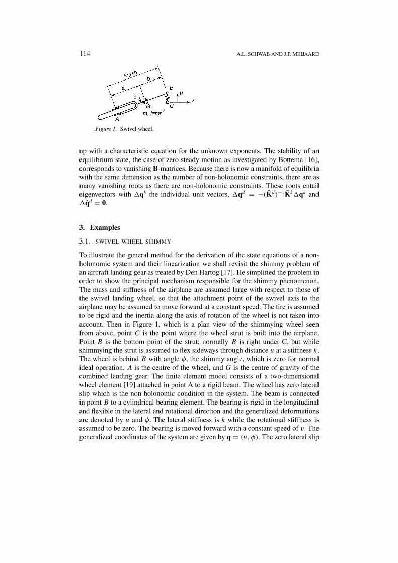
Figure 1. Swivel wheel.

up with a characteristic equation for the unknown exponents. The stability of anequilibrium state, the case of zero steady motion as investigated by Bottema [16],corresponds to vanishing B-matrices. Because there is now a manifold of equilibriawith the same dimension as the number of non-holonomic constraints, there are asmany vanishing roots as there are non-holonomic constraints. These roots entaileigenvectors with �qk the individual unit vectors, �qd = −(Kd)−1Kk�qk and�qd = 0.

3. Examples

3.1. SWIVEL WHEEL SHIMMY

To illustrate the general method for the derivation of the state equations of a non-holonomic system and their linearization we shall revisit the shimmy problem ofan aircraft landing gear as treated by Den Hartog [17]. He simplified the problem inorder to show the principal mechanism responsible for the shimmy phenomenon.The mass and stiffness of the airplane are assumed large with respect to those ofthe swivel landing wheel, so that the attachment point of the swivel axis to theairplane may be assumed to move forward at a constant speed. The tire is assumedto be rigid and the inertia along the axis of rotation of the wheel is not taken intoaccount. Then in Figure 1, which is a plan view of the shimmying wheel seenfrom above, point C is the point where the wheel strut is built into the airplane.Point B is the bottom point of the strut; normally B is right under C, but whileshimmying the strut is assumed to flex sideways through distance u at a stiffness k.The wheel is behind B with angle φ, the shimmy angle, which is zero for normalideal operation. A is the centre of the wheel, and G is the centre of gravity of thecombined landing gear. The finite element model consists of a two-dimensionalwheel element [19] attached in point A to a rigid beam. The wheel has zero lateralslip which is the non-holonomic condition in the system. The beam is connectedin point B to a cylindrical bearing element. The bearing is rigid in the longitudinaland flexible in the lateral and rotational direction and the generalized deformationsare denoted by u and φ. The lateral stiffness is k while the rotational stiffness isassumed to be zero. The bearing is moved forward with a constant speed of v. Thegeneralized coordinates of the system are given by q = (u, φ). The zero lateral slip


condition on the wheel reduces the coordinates to the degree of freedom qd = (u)

and the kinematic coordinate qk = (φ). The steady state undeformed motion ischaracterized by (u, u, φ) = (0, 0, 0). With the variations �qd = �u, �qd = �u

and �qk = �φ, the coefficients of the linearized state derivatives according to (29)are

M = m

(a2 + r2

l2

),

C = m

(ab − r2

l2

)v

l, A = 1

l,

Kd = k, Bd = 0,

Kk = −m

(ab − r2

l2

)v2

l, Bk = −v

l,

f = 0. (30)

These coefficients are usually numerically calculated by the program but wepresent them here in an analytical form so we can compare them with the approachas presented by Den Hartog [17]. His ad hoc analysis leads to an eigenvalue prob-lem. The systematically derived linearized state derivatives (30) lead to the sameeigenvalue problem and consequently to the same prediction of unstable shimmybehaviour.

To investigate the shimmy motion we start with the usual assumption of anexponential motion for the small variations �q of the form �q0 exp(λt). The char-acteristic equation of the eigenvalue problem from (29) with the coefficients from(30) is

λ3 + (1 + µ)ωλ2 + ω2nλ + ωω2

n = 0, (31)

with the mass distribution factor µ = (ab − r2)/(a2 + r2), the driving frequencyω = v/l and the natural frequency ωn = √

kl2/(m(a2 + r2)). A neccessary andsufficient condition for asymptotic stability is given by the requirement that allroots of (31) have negative real parts. Application of Hurwitz’s theorem on thecharacteristic equation (31) yields

ω > 0 and µ > 0. (32)

In other words, the motion is stable if the driving speed v is positive and the centreof mass is positioned such that a(l − a) > r2. The latter corresponds to a region of±√

(l/2)2 − r2 around the midpoint a = l/2. For the critical case, where a(l−a) =r2, there is one real eigenvalue λ1 = −ω describing the non-oscillating decayingmotion and a pair of conjugated imaginary values λ2,3 = ±ωni which describe theundamped oscillatory solution. This critical case corresponds to a mass distributionwhere point B is the centre of percussion or in other words, the lateral contact forcein A has no influence on the lateral spring force in B.


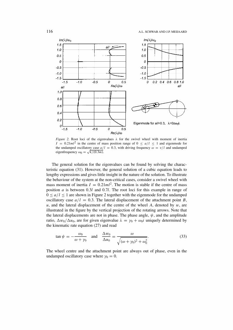
Figure 2. Root loci of the eigenvalues λ for the swivel wheel with moment of inertiaI = 0.21ml2 in the centre of mass position range of 0 ≤ a/l ≤ 1 and eigenmode forthe undamped oscillatory case a/l = 0.3, with driving frequency ω = v/l and undampedeigenfrequency ω0 = √

k/(0.3m).

The general solution for the eigenvalues can be found by solving the charac-teristic equation (31). However, the general solution of a cubic equation leads tolengthy expressions and gives little insight in the nature of the solution. To illustratethe behaviour of the system at the non-critical cases, consider a swivel wheel withmass moment of inertia I = 0.21ml2. The motion is stable if the centre of massposition a is between 0.3l and 0.7l. The root loci for this example in range of0 ≤ a/l ≤ 1 are shown in Figure 2 together with the eigenmode for the undampedoscillatory case a/l = 0.3. The lateral displacement of the attachment point B,u, and the lateral displacement of the centre of the wheel A, denoted by w, areillustrated in the figure by the vertical projection of the rotating arrows. Note thatthe lateral displacements are not in phase. The phase angle, ψ , and the amplituderatio, �w0/�u0, are for given eigenvalue λ = γ0 + ω0i uniquely determined bythe kinematic rate equation (27) and read

tan ψ = − ω0

ω + γ0and

�w0

�u0= ω√

(ω + γ0)2 + ω20

. (33)

The wheel centre and the attachment point are always out of phase, even in theundamped oscillatory case where γ0 = 0.


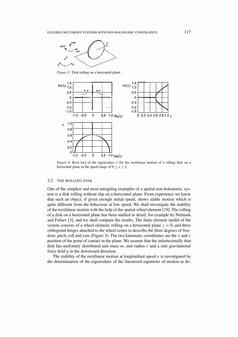
Figure 3. Disk rolling on a horizontal plane.

Figure 4. Root loci of the eigenvalues λ for the rectilinear motion of a rolling disk on ahorizontal plane in the speed range of 0 ≤ v ≤ 1.

3.2. THE ROLLING DISK

One of the simplest and most intriguing examples of a spatial non-holonomic sys-tem is a disk rolling without slip on a horizontal plane. From experience we knowthat such an object, if given enough initial speed, shows stable motion which isquite different from the behaviour at low speed. We shall investigate the stabilityof the rectilinear motion with the help of the spatial wheel element [19]. The rollingof a disk on a horizontal plane has been studied in detail, for example by Neımarkand Fufaev [3], and we shall compare the results. The finite element model of thesystem consists of a wheel element, rolling on a horizontal plane z = 0, and threeorthogonal hinges attached to the wheel centre to describe the three degrees of free-dom: pitch, roll and yaw (Figure 3). The two kinematic coordinates are the x and y

position of the point of contact in the plane. We assume that the infinitesimally thindisk has uniformly distributed unit mass m, unit radius r and a unit gravitationalforce field g in the downward direction.

The stability of the rectilinear motion at longitudinal speed v is investigated bythe determination of the eigenvalues of the linearized equations of motion as de-


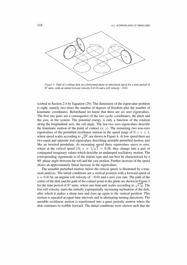
Figure 5. Path of a rolling disk on a horizontal plane at subcritical speed for a time period of87 units, with an initial forward velocity 0.4116 and a roll velocity −0.01.

scribed in Section 2.4 by Equation (29). The dimension of the eigenvalue problemis eight; namely two times the number of degrees of freedom plus the number ofkinematic coordinates. Beforehand we know that there are six zero eigenvalues.The first two pairs are a consequence of the two cyclic coordinates, the pitch andthe yaw, in the system. The potential energy is only a function of the rotationalong the longitudinal axis, the roll angle. The last two zero eigenvalues describethe kinematic motion of the point of contact (x, y). The remaining two non-zeroeigenvalues of the perturbed rectilinear motion in the speed range of 0 ≤ v ≤ 1,where speed scales according to

√gr , are shown in Figure 4. At low speed there are

two equal and opposite real eigenvalues describing unstable perturbed motion, justlike an inverted pendulum. At increasing speed these eigenvalues move to zero,where at the critical speed [3], v = 1/

√3 ≈ 0.58, they change into a pair of

conjugated imaginary values which describe an undamped oscillatory motion. Thecorresponding eigenmode is of the slalom type and can best be characterised by a90◦ phase angle between the roll and the yaw motion. Further increase of the speedshows an approximately linear increase in the eigenvalues.

The unstable perturbed motion, below the critical speed, is illustrated by a tran-sient analysis. The initial conditions are a vertical position with a forward speed ofv = 0.4116, an angular roll velocity of −0.01 and a zero yaw rate. The path of thecentre of the disk and the path of the contact point in the plane are shown in Figure 5for the time period of 87 units, where one time unit scales according to

√r/g. The

low roll velocity starts the initially exponentially increasing inclination of the disk,after which it makes a sharp turn and rises up again to the vertical position. Thismotion is repeated at equal time intervals and in alternating turning directions. Theunstable rectilinear motion is transformed into a quasi periodic motion where thedisk continues to wobble forward. The initial conditions were chosen such that the


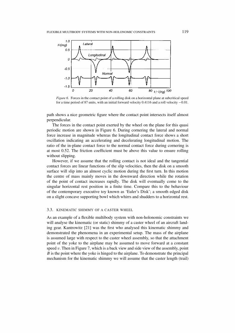
Figure 6. Forces in the contact point of a rolling disk on a horizontal plane at subcritical speedfor a time period of 87 units, with an initial forward velocity 0.4116 and a roll velocity −0.01.

path shows a nice geometric figure where the contact point intersects itself almostperpendicular.

The forces in the contact point exerted by the wheel on the plane for this quasiperiodic motion are shown in Figure 6. During cornering the lateral and normalforce increase in magnitude whereas the longitudinal contact force shows a shortoscillation indicating an accelerating and decelerating longitudinal motion. Theratio of the in-plane contact force to the normal contact force during cornering isat most 0.52. The friction coefficient must be above this value to ensure rollingwithout slipping.

However, if we assume that the rolling contact is not ideal and the tangentialcontact forces are linear functions of the slip velocities, then the disk on a smoothsurface will slip into an almost cyclic motion during the first turn. In this motionthe centre of mass mainly moves in the downward direction while the rotationof the point of contact increases rapidly. The disk will eventually come to thesingular horizontal rest position in a finite time. Compare this to the behaviourof the contemporary executive toy known as ‘Euler’s Disk’; a smooth edged diskon a slight concave supporting bowl which whirrs and shudders to a horizontal rest.

3.3. KINEMATIC SHIMMY OF A CASTER WHEEL

As an example of a flexible multibody system with non-holonomic constraints wewill analyse the kinematic (or static) shimmy of a caster wheel of an aircraft land-ing gear. Kantrowitz [21] was the first who analysed this kinematic shimmy anddemonstrated the phenomena in an experimental setup. The mass of the airplaneis assumed large with respect to the caster wheel assembly, so that the attachmentpoint of the yoke to the airplane may be assumed to move forward at a constantspeed v. Then in Figure 7, which is a back view and side view of the assembly, pointB is the point where the yoke is hinged to the airplane. To demonstrate the principalmechanism for the kinematic shimmy we will assume that the caster length (trail)


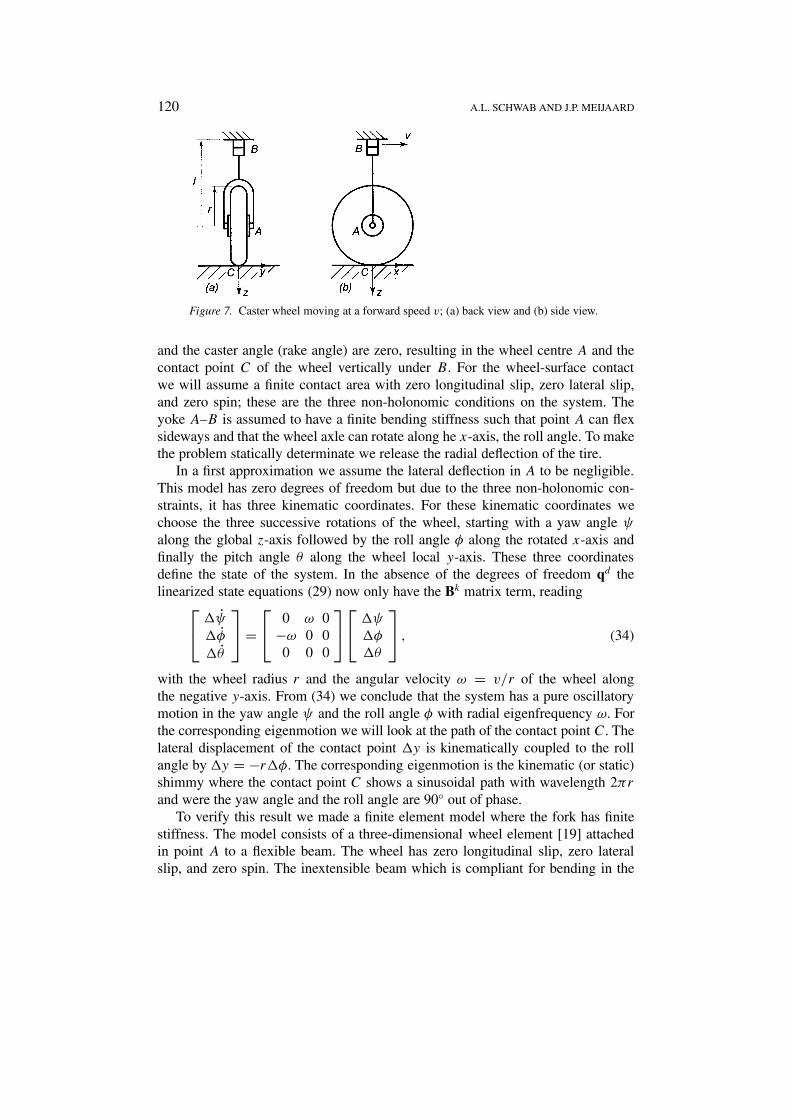
Figure 7. Caster wheel moving at a forward speed v; (a) back view and (b) side view.

and the caster angle (rake angle) are zero, resulting in the wheel centre A and thecontact point C of the wheel vertically under B. For the wheel-surface contactwe will assume a finite contact area with zero longitudinal slip, zero lateral slip,and zero spin; these are the three non-holonomic conditions on the system. Theyoke A–B is assumed to have a finite bending stiffness such that point A can flexsideways and that the wheel axle can rotate along he x-axis, the roll angle. To makethe problem statically determinate we release the radial deflection of the tire.

In a first approximation we assume the lateral deflection in A to be negligible.This model has zero degrees of freedom but due to the three non-holonomic con-straints, it has three kinematic coordinates. For these kinematic coordinates wechoose the three successive rotations of the wheel, starting with a yaw angle ψ

along the global z-axis followed by the roll angle φ along the rotated x-axis andfinally the pitch angle θ along the wheel local y-axis. These three coordinatesdefine the state of the system. In the absence of the degrees of freedom qd thelinearized state equations (29) now only have the Bk matrix term, reading

�ψ

�φ

�θ

=

0 ω 0

−ω 0 00 0 0

�ψ

�φ

�θ

, (34)

with the wheel radius r and the angular velocity ω = v/r of the wheel alongthe negative y-axis. From (34) we conclude that the system has a pure oscillatorymotion in the yaw angle ψ and the roll angle φ with radial eigenfrequency ω. Forthe corresponding eigenmotion we will look at the path of the contact point C. Thelateral displacement of the contact point �y is kinematically coupled to the rollangle by �y = −r�φ. The corresponding eigenmotion is the kinematic (or static)shimmy where the contact point C shows a sinusoidal path with wavelength 2πr

and were the yaw angle and the roll angle are 90◦ out of phase.To verify this result we made a finite element model where the fork has finite

stiffness. The model consists of a three-dimensional wheel element [19] attachedin point A to a flexible beam. The wheel has zero longitudinal slip, zero lateralslip, and zero spin. The inextensible beam which is compliant for bending in the


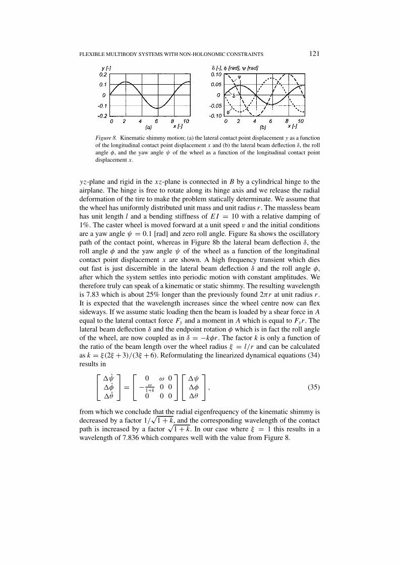
Figure 8. Kinematic shimmy motion; (a) the lateral contact point displacement y as a functionof the longitudinal contact point displacement x and (b) the lateral beam deflection δ, the rollangle φ, and the yaw angle ψ of the wheel as a function of the longitudinal contact pointdisplacement x.

yz-plane and rigid in the xz-plane is connected in B by a cylindrical hinge to theairplane. The hinge is free to rotate along its hinge axis and we release the radialdeformation of the tire to make the problem statically determinate. We assume thatthe wheel has uniformly distributed unit mass and unit radius r. The massless beamhas unit length l and a bending stiffness of EI = 10 with a relative damping of1%. The caster wheel is moved forward at a unit speed v and the initial conditionsare a yaw angle ψ = 0.1 [rad] and zero roll angle. Figure 8a shows the oscillatorypath of the contact point, whereas in Figure 8b the lateral beam deflection δ, theroll angle φ and the yaw angle ψ of the wheel as a function of the longitudinalcontact point displacement x are shown. A high frequency transient which diesout fast is just discernible in the lateral beam deflection δ and the roll angle φ,after which the system settles into periodic motion with constant amplitudes. Wetherefore truly can speak of a kinematic or static shimmy. The resulting wavelengthis 7.83 which is about 25% longer than the previously found 2πr at unit radius r.It is expected that the wavelength increases since the wheel centre now can flexsideways. If we assume static loading then the beam is loaded by a shear force in A

equal to the lateral contact force Fy and a moment in A which is equal to Fyr. Thelateral beam deflection δ and the endpoint rotation φ which is in fact the roll angleof the wheel, are now coupled as in δ = −kφr. The factor k is only a function ofthe ratio of the beam length over the wheel radius ξ = l/r and can be calculatedas k = ξ(2ξ +3)/(3ξ +6). Reformulating the linearized dynamical equations (34)results in

�ψ

�φ

�θ

=

0 ω 0

− ω1+k

0 00 0 0

�ψ

�φ

�θ

, (35)

from which we conclude that the radial eigenfrequency of the kinematic shimmy isdecreased by a factor 1/

√1 + k, and the corresponding wavelength of the contact

path is increased by a factor√

1 + k. In our case where ξ = 1 this results in awavelength of 7.836 which compares well with the value from Figure 8.


4. Conclusion

A procedure has been described for formulating the dynamical equations of non-holonomic mechanical systems as well as their linearized equations. The procedurecan be applied to systems with flexible bodies with the same ease as to systems withrigid bodies. Advantages of the procedure are the use of a set of minimal independ-ent state variables, which avoid the use of differential-algebraic equations, and theanalytic linearization, which is more accurate than numerical differentiation. Thelinearized equations can be used to analyse the stability of a nominal steady motion.

References

1. Lagrange, J.L., Analytical Mechanics, Kluwer, Dordrecht, 1997. (Original French first edi-tion Méchanique analitique, Desaint, Paris, 1788.) (Translated from the French second editionMécanique analytique, Courcier, Paris, 1811, by A. Boissonnade and V.N. Vagliente.)

2. Hertz, H., Die Prinzipien der Mechanik in neuem Zusammenhange dargestellt, JohannAmbrosius Barth, Leipzig, 1894.

3. Neımark, Ju.I. and Fufaev, N.A., Dynamics of Nonholonomic Systems, American MathematicalSociety, Providence, RI, 1972. (Translated from the Russian edition, Nauka, Moscow, 1967.)

4. Kreuzer, E.J., ‘Symbolische Berechnung der Bewegungsgleichungen von Mehrkörpersyste-men’, Dissertation, Fortschrittberichte der VDI Zeitschriften, Reihe 11, Nr. 32, 1979.

5. Nikravesh, P.E. and Haug, E.J., ‘Generalized coordinate partitioning for analysis of mechanicalsystems with nonholonomic constraints’, ASME Journal of Mechanisms, Transmissions, andAutomation in Design 105, 1983, 379–384.

6. Schwab, A.L. and Meijaard, J.P., ‘Small vibrations superimposed on a prescribed rigid bodymotion’, Multibody System Dynamics 8, 2002, 29–49.

7. Besseling, J.F., ‘The complete analogy between the matrix equations and the continuous fieldequations of structural analysis’, in International Symposium on Analogue and Digital Tech-niques Applied to Aeronautics: Proceedings, Presses Académiques Européennes, Bruxelles,1964, 223–242.

8. Van der Werff, K., ‘Kinematic and dynamic analysis of mechanisms, A finite elementapproach’, Dissertation, Delft University Press, Delft, 1977.

9. Jonker, J.B., ‘A finite element dynamic analysis of flexible spatial mechanisms and manipulat-ors’, Dissertation, Delft University Press, Delft, 1988.

10. Cardona, A., Géradin, M. and Doan, D.B., ‘Rigid and flexible joint modeling in multibodydynamics using finite-elements’, Computer Methods in Applied Mechanics and Engineering89, 1991, 395–418.

11. Géradin, M. and Cardona, A., Flexible Multibody Dynamics: A Finite Element Approach,Wiley, Chichester, 2001.

12. Meijaard, J.P., ‘Direct determination of periodic solutions of the dynamical equations of flexiblemechanisms and manipulators’, International Journal for Numerical Methods in Engineering32, 1991, 1691–1710.

13. Schwab, A.L., ‘Dynamics of flexible multibody systems’, Dissertation, Delft University ofTechnology, Delft, April 2002.

14. Jonker, J.B. and Meijaard, J.P., ‘SPACAR – Computer program for dynamic analysis of flexiblespatial mechanisms and manipulators’, in Multibody Systems Handbook, W. Schiehlen (ed.),Springer-Verlag, Berlin, 1990, 123–143.

15. Whittaker, E.T., A Treatise on the Analytical Dynamics of Particles and Rigid Bodies, fourthedition, Cambridge University Press, Cambridge, U.K., 1937.


16. Bottema, O., ‘On the small vibration of non-holonomic systems’, Proceedings KoninklijkeNederlandse Akademie van Wetenschappen 52, 1949, 848–850.

17. Den Hartog, J.P., Mechanical Vibrations, fourth edition, McGraw-Hill, New York, 1956.18. Schwab, A.L. and Meijaard, J.P., ‘The belt, gear, bearing and hinge as special finite elements

for kinematic and dynamic analysis of mechanisms and machines’, in Leinonen, T. (ed.), Pro-ceedings of the Tenth World Congress on the Theory of Machines and Mechanisms, IFToMM,June 20–24, Oulu, Finland, Oulu University Press, 1999, Vol. 4, 1375–1386.

19. Schwab, A.L. and Meijaard, J.P., ‘Dynamics of flexible multibody systems having rollingcontact: Application of the wheel element to the dynamics of road vehicles’, Vehicle SystemDynamics Supplement 33, 1999, 338–349.

20. Schwab, A.L. and Meijaard, J.P., ‘Two special finite elements for modelling rolling contactin a multibody environment’, in Proceedings of the First Asian Conference on Multibody Dy-namics, ACMD’02, July 31–August 2, 2002, Iwaki, Fukushima, Japan, The Japan Society ofMechanical Engineering, 2002, 386–391.

21. Kantrowitz, A., ‘Stability of castering wheels for aircraft landing gears’, Technical Report 686,NACA, Washington DC, 1940, 147–162.

Documents

Dynamics of Flexible Multibody Systems with Non-Holonomic Constraints: A Finite Element Approach