Embed Size (px)
Citation preview
Software User's Manual
1
EC-Lab/BT-Lab® Software
User's Manual
January 2017
Software User's Manual
2
Table of contents
1. Introduction ..................................................................................................................... 5
2. Overview.......................................................................................................................... 7
2.1 Starting the software ................................................................................................ 7
2.2 Global view ............................................................................................................... 8
2.3 Main Menu ............................................................................................................... 9
2.4 Tool Bars ................................................................................................................ 12
2.4.1 Main Tool Bar ..................................................................................................... 12 2.4.2 Channel Tool bar ................................................................................................ 13 2.4.3 Graph Tool Bar ................................................................................................... 13 2.4.4 Status Tool Bar ................................................................................................... 14 2.4.5 Current Values Tool Bar ..................................................................................... 14
2.5 Devices box ............................................................................................................ 15
2.6 Experiments box .................................................................................................... 16
2.6.1 Advanced Settings tab ........................................................................................ 16 2.6.1.1 Advanced Settings for VMP3, VSP, SP-50, SP-150 ................................... 16
2.6.1.1.1 Compliance ........................................................................................... 17 2.6.1.1.2 Safety Limits ......................................................................................... 18 2.6.1.1.3 Electrode Connections .......................................................................... 19 2.6.1.1.4 Miscellaneous ....................................................................................... 19
2.6.1.2 Advanced Settings for HCP-, CLB- MPG-2xx series .................................. 21 2.6.1.3 Advanced Settings for VMP-300 based instruments .................................. 21
2.6.1.3.1 Filtering ................................................................................................. 22 2.6.1.3.2 Channel ................................................................................................. 22 2.6.1.3.3 Ultra Low Current Option ...................................................................... 22 2.6.1.3.4 Electrode Connections .......................................................................... 24
2.6.1.4 Advanced Settings for BCS-8xx series instruments ................................... 26 2.6.2 Cell Characteristics Tab ...................................................................................... 26
2.6.2.1 Cell Description ........................................................................................... 27 2.6.2.1.1 Standard “Cell Description” frame ......................................................... 27 2.6.2.1.2 Battery “Cell Description” frame ............................................................ 29 2.6.2.1.3 Corrosion “Cell Description” frame ........................................................ 31
2.6.2.2 Reference electrode.................................................................................... 32 2.6.2.3 Record ........................................................................................................ 33
2.6.3 Parameters Settings Tab .................................................................................... 33 2.6.3.1 Right-click on the “Parameters Settings” tab .............................................. 34 2.6.3.2 Selecting a technique.................................................................................. 35 2.6.3.3 Changing the parameters of a technique .................................................... 36
2.7 Accepting and saving settings and running an experiment .................................... 39
2.7.1 Accepting and saving settings ............................................................................ 39 2.7.2 Running an experiment....................................................................................... 40 2.7.3 Restore ............................................................................................................... 40
2.8 Linking techniques ................................................................................................. 41
2.8.1 Description and settings ..................................................................................... 41 2.8.2 Applications ........................................................................................................ 43
2.8.2.1 Linked experiments with EIS techniques .................................................... 43 2.8.2.2 Application of linked experiments with ohmic drop compensation .............. 45
2.9 Available commands during the run ....................................................................... 45
2.9.1 Stop and Pause .................................................................................................. 45
Software User's Manual
3
2.9.2 Next Technique/Next Sequence ......................................................................... 46 2.9.3 Modifying an experiment in progress .................................................................. 46 2.9.4 Repair channel ................................................................................................... 46
2.9.4.1 Use of the Repair channel tool .................................................................... 47
2.10 Grouped & Synchronized experiments .................................................................. 49
2.11 Stack experiments .................................................................................................. 51
2.12 Parallel configuration .............................................................................................. 53
2.13 Batch mode ............................................................................................................ 54
2.14 Data properties ....................................................................................................... 55
2.14.1 Type of data files ............................................................................................ 55 2.14.2 Variables description ...................................................................................... 56 2.14.3 Data recording ................................................................................................ 57 2.14.4 Data saving ..................................................................................................... 58
2.15 Changing the channel owner ................................................................................. 58
2.16 Virtual potentiostat ................................................................................................. 59
2.17 Configuration options ............................................................................................. 60
2.17.1 General Options .............................................................................................. 60 2.17.2 Warning Options ............................................................................................. 61 2.17.3 Text Export Options ........................................................................................ 62 2.17.4 Color Options .................................................................................................. 62 2.17.5 References Options ........................................................................................ 63 2.17.6 Tool bars/menus Options ................................................................................ 64 2.17.7 E-mail/menus Options .................................................................................... 64
3. Graphic Display ............................................................................................................ 66
3.1 Graphic window ...................................................................................................... 66
3.1.1 Loading a data file .............................................................................................. 68 3.1.2 Example with a CV ............................................................................................. 69 3.1.3 Graphic tool bar .................................................................................................. 70 3.1.4 Data file and plot selection window ..................................................................... 70
3.2 Graphic tools .......................................................................................................... 71
3.2.1 Cycles/Loops visualization .................................................................................. 71 3.2.2 Show/Hide points ................................................................................................ 73 3.2.3 Add comments on the graph ............................................................................... 73 3.2.4 Three-Dimensional graphic ................................................................................. 75 3.2.5 Graph properties ................................................................................................. 76 3.2.6 LOG (History) file ................................................................................................ 79 3.2.7 Copy options ....................................................................................................... 81
3.2.7.1 Standard copy options ................................................................................ 81 3.2.7.2 Advanced copy options ............................................................................... 81
3.2.8 Print options ........................................................................................................ 81 3.2.9 Multi-graphs in a window .................................................................................... 83
3.2.9.1 Multi windows.............................................................................................. 83 3.2.10 Graph Representation menu .......................................................................... 84
3.2.10.1 Axis processing ....................................................................................... 85 3.2.10.2 How to create your own graph representation for a specific technique? 86 3.2.10.3 How to create a Graph Style? ................................................................. 87
4. Data File import/export functions ............................................................................... 90
4.1.1 ASCII text file creation and exportation .............................................................. 90 4.1.1.1 Template ..................................................................................................... 91
4.1.2 ASCII text file importation from other electrochemical software ......................... 91
Software User's Manual
4
4.1.3 Append file. ......................................................................................................... 93 4.1.4 FC-Lab data files importation .............................................................................. 93
5. External device control and recording ....................................................................... 94
5.1 General description ................................................................................................ 94
5.2 Rotating electrodes control .................................................................................... 95
5.3 Temperature control ............................................................................................... 98
5.4 Electrochemical Quartz Crystal Microbalance ....................................................... 98
6. Troubleshooting ......................................................................................................... 100
6.1 In case of problem ................................................................................................ 100
6.2 Data saving .......................................................................................................... 101
6.3 PC Disconnection ................................................................................................. 101
6.4 Effect of computer save options on data recording .............................................. 101
7. Glossary ...................................................................................................................... 102
8. Index ............................................................................................................................ 108
9. List of Notes ................................................................................................................ 111
9.1 Application Notes ................................................................................................. 111
9.2 Technical Notes ................................................................................................... 113
Software User's Manual
5
1. Introduction
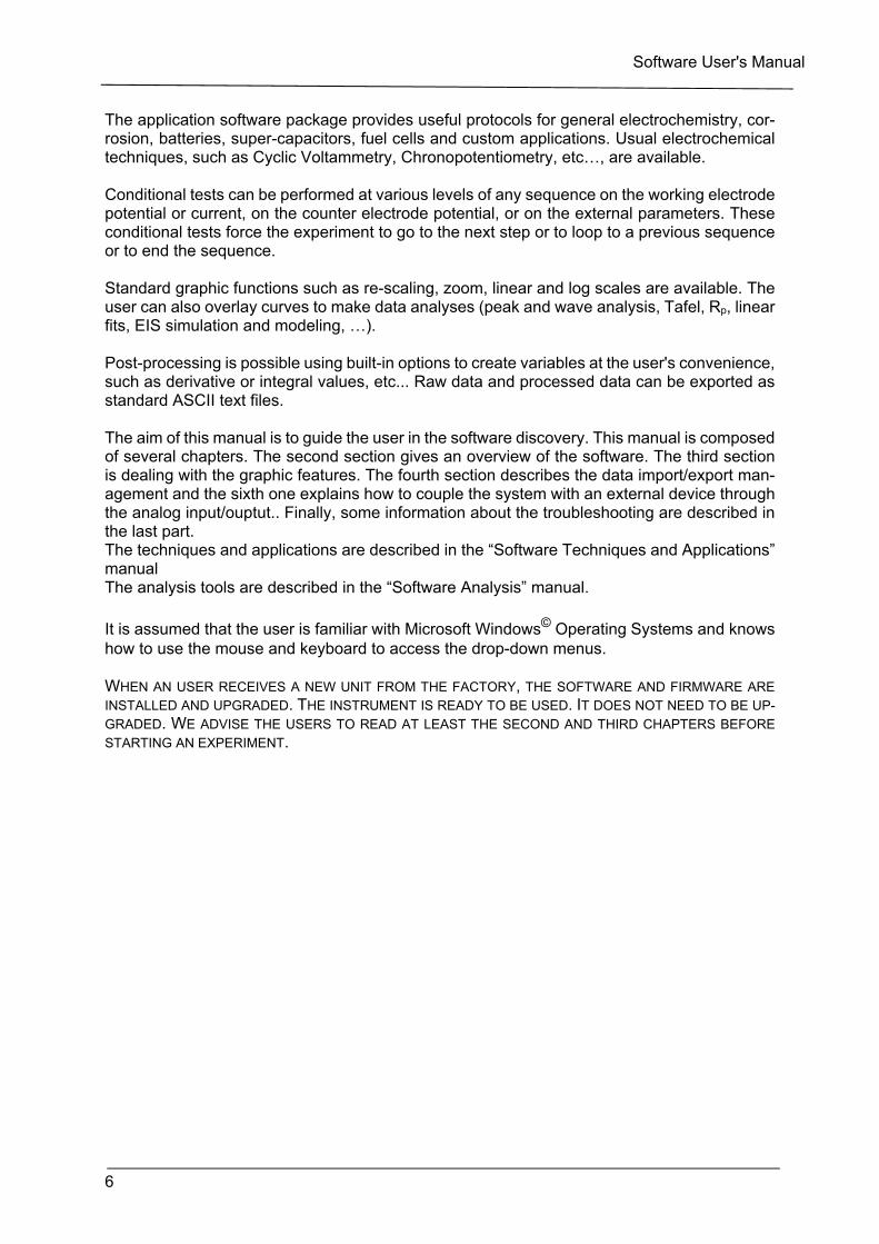
Bio-Logic’s software, EC-Lab® and BT-Lab®, have been designed and built to control Bio-Logic’s potentiostats/glavanostat and cyclers. EC-Lab® is general purpose software and can control a wide range of potentiostat/gal-vanostat/EIS instruments whereas BT-Lab® is dedicated to battery cycling. The compatibilities between instrument and software are given in the table below:
Tab. 1: Software compatibilities.
Type of instruments
Technology Instruments EC-Lab® BT-Lab®
Single channel
VMP3 based VMP3 based VMP-300 based VMP-300 based VMP-300 based
SP-50 SP-150 SP-200 SP-240 SP-300
√ √ √ √ √
Multichannel
VMP3 based VMP3 based VMP3 based VMP-300 based VMP-300 based
VSP VMP2 VMP3 VSP-300 VMP-300
√ √ √ √ √
High Power VMP3 based
VMP3 based VMP3 based
HCP-803 HCP-1005 CLB-2000
√ √ √
Battery cyclers VMP3 based
BCS based MPG-2xx BCS-8xx series
√ √
Each channel board of our multichannel instruments is an independent potentiostat/gal-vanostat/EIS. Each channel can be set, run, paused or stopped, independently of each other, using identical or different protocols. Any settings of any channel can be modified during a run, without inter-rupting the experiment. The channels can be interconnected and run synchronously. One computer (or eventually several for multichannel instruments, up to 16) connected to the instrument can monitor the system. The computer can be connected to the instrument through an Ethernet connection or with an USB connection (only for EC-Lab®). With the Ethernet con-nection, each user is able to monitor his own channel from his computer. Our instruments are modular, versatile and flexible multi-user instruments. Additionally, several instruments can be controlled by one computer with only one session open. Once the protocols have been loaded and started from the PC, the experiments are entirely controlled by the on-board firmware of the instrument. Data are temporarily buffered in the instrument and regularly transferred to the PC, which is used for data storage, on-line visuali-zation and off-line data analysis and display. This architecture ensures very safe operations since a shutdown of the monitoring PC does not affect the experiments in progress.
Software User's Manual
6
The application software package provides useful protocols for general electrochemistry, cor-rosion, batteries, super-capacitors, fuel cells and custom applications. Usual electrochemical techniques, such as Cyclic Voltammetry, Chronopotentiometry, etc…, are available. Conditional tests can be performed at various levels of any sequence on the working electrode potential or current, on the counter electrode potential, or on the external parameters. These conditional tests force the experiment to go to the next step or to loop to a previous sequence or to end the sequence. Standard graphic functions such as re-scaling, zoom, linear and log scales are available. The user can also overlay curves to make data analyses (peak and wave analysis, Tafel, Rp, linear fits, EIS simulation and modeling, …). Post-processing is possible using built-in options to create variables at the user's convenience, such as derivative or integral values, etc... Raw data and processed data can be exported as standard ASCII text files. The aim of this manual is to guide the user in the software discovery. This manual is composed of several chapters. The second section gives an overview of the software. The third section is dealing with the graphic features. The fourth section describes the data import/export man-agement and the sixth one explains how to couple the system with an external device through the analog input/ouptut.. Finally, some information about the troubleshooting are described in the last part. The techniques and applications are described in the “Software Techniques and Applications” manual The analysis tools are described in the “Software Analysis” manual.
It is assumed that the user is familiar with Microsoft Windows© Operating Systems and knows how to use the mouse and keyboard to access the drop-down menus. WHEN AN USER RECEIVES A NEW UNIT FROM THE FACTORY, THE SOFTWARE AND FIRMWARE ARE
INSTALLED AND UPGRADED. THE INSTRUMENT IS READY TO BE USED. IT DOES NOT NEED TO BE UP-
GRADED. WE ADVISE THE USERS TO READ AT LEAST THE SECOND AND THIRD CHAPTERS BEFORE
STARTING AN EXPERIMENT.
Software User's Manual
7
2. Overview
At this point, the installation manual of your instrument has been carefully read and the user knows how to connect his/her instrument to the instruments. The several steps of the connection will not be described in this manual but in the installation manual of the instrument.
2.1 Starting the software
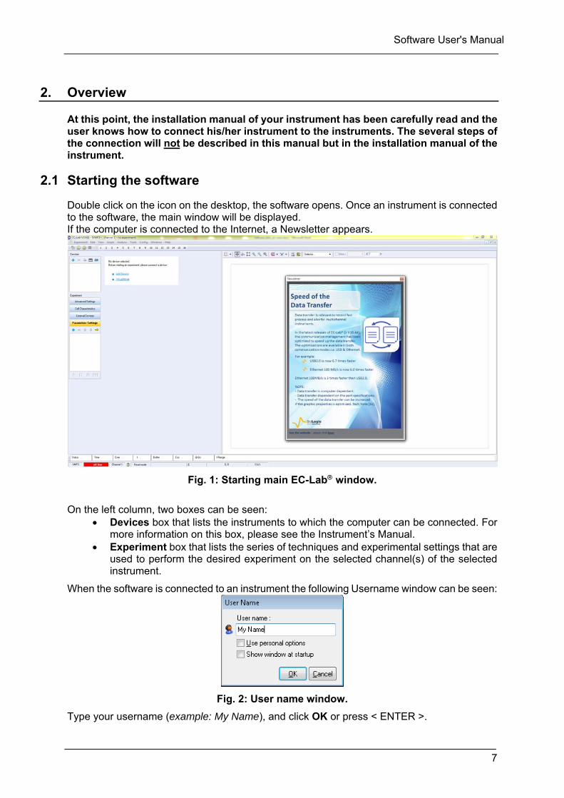
Double click on the icon on the desktop, the software opens. Once an instrument is connected to the software, the main window will be displayed. If the computer is connected to the Internet, a Newsletter appears.
Fig. 1: Starting main EC-Lab window.
On the left column, two boxes can be seen:
Devices box that lists the instruments to which the computer can be connected. For more information on this box, please see the Instrument’s Manual.
Experiment box that lists the series of techniques and experimental settings that are used to perform the desired experiment on the selected channel(s) of the selected instrument.
When the software is connected to an instrument the following Username window can be seen:
Fig. 2: User name window.
Type your username (example: My Name), and click OK or press < ENTER >.
Software User's Manual
8
This User Name is used as a safety password when the instrument is shared between several users. When you run an experiment on a channel, this code will be automatically transferred to the section "user" on the bottom of the software window. This allows the user to become the owner of the channel for the duration of the experiment. All users are authorized to view the channels owned by the other users. However, change of parameters on a channel is author-ized only if the present User Name corresponds to the owner of that channel (even from an-other computer). If another user wants to modify parameters on a channel that belongs to "My Name", the following message appears: "Warning, channel X belongs to "My Name". By accepting modification you will replace current owner. Do you want to continue?"
The command User... in the Config. menu allows you to change the User Name at any time. You can also double click on the “User“section in the bottom of the software window to change the User Name. The user can specify a personal configuration (color display, tool bar buttons and position, default settings), which is linked to the User Name. If it is not selected, the default configuration is used. For the user’s convenience it is also possible to hide this window when the software is starting. This window shows at the very top, in the blue title bar: the software version, the connected instrument, the IP address (if connected through a LAN), the active channel, the name of the experiment (i.e. name of the data file) and the selected technique (if any).
2.2 Global view
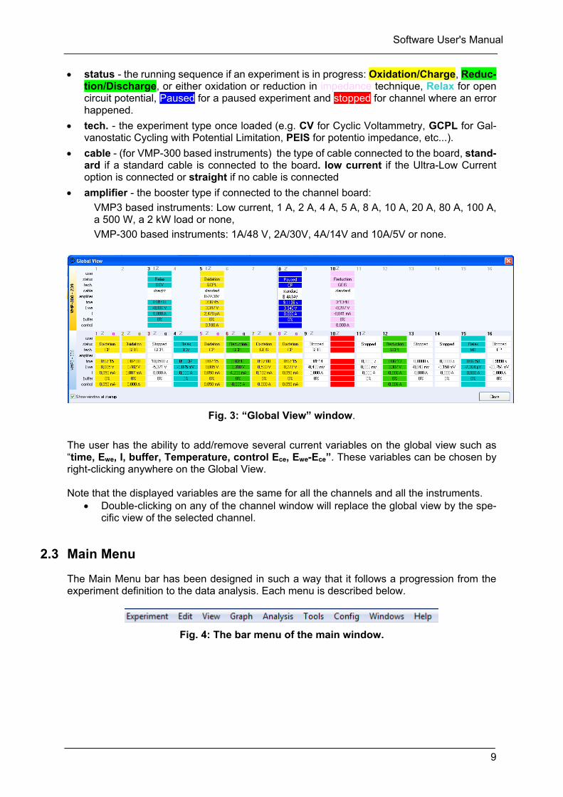
Once your instruments are connected, you can have all the details about the experiments by accessing the Global View. There are several ways to access the Global View window:
1. It automatically appears once the User Name is set the first time the software is opened.
2. In the Devices box, click on 3. Press Ctrl+W 4. Go to View\Global View
The global view of the channels shows the following information:
On the left the instruments (EC-Lab®) or BCS-8xx modules (BT-Lab®) to which the com-puter is connected. The active or selected instrument will appear in a different color.
channel number with Z if impedance option is available on the channel.
If the channels are synchronized, grouped, or execute a stack, a bipotentiostat technique, they will appear in a different color.
letter “l” is displayed near the channel number when a Analog Ramp Generator is added to a channel board (for VMP-300 based instruments). letter ”s” is displayed in the left side of the channel column if a channel is syn-chronized with other channels. letter “g” is displayed in the left side of the channel column if a channel is grouped with other channels.
an indicative ‘BAR’ in -white if there is no experiment running, colored if the channel is running. If no pstat board, booster or low current board inserted in a slot, the corresponding slot number is greyed out and no information is displayed on the global View window.
user - the channel is available (no username) or is (was) used by another user. Several users can be connected to the instrument, each user can work on one or several channels.
Software User's Manual
9
status - the running sequence if an experiment is in progress: Oxidation/Charge, Reduc-tion/Discharge, or either oxidation or reduction in impedance technique, Relax for open circuit potential, Paused for a paused experiment and stopped for channel where an error happened.
tech. - the experiment type once loaded (e.g. CV for Cyclic Voltammetry, GCPL for Gal-vanostatic Cycling with Potential Limitation, PEIS for potentio impedance, etc...).
cable - (for VMP-300 based instruments) the type of cable connected to the board, stand-ard if a standard cable is connected to the board. low current if the Ultra-Low Current option is connected or straight if no cable is connected
amplifier - the booster type if connected to the channel board:
VMP3 based instruments: Low current, 1 A, 2 A, 4 A, 5 A, 8 A, 10 A, 20 A, 80 A, 100 A, a 500 W, a 2 kW load or none,
VMP-300 based instruments: 1A/48 V, 2A/30V, 4A/14V and 10A/5V or none.
Fig. 3: “Global View” window.
The user has the ability to add/remove several current variables on the global view such as “time, Ewe, I, buffer, Temperature, control Ece, Ewe-Ece”. These variables can be chosen by right-clicking anywhere on the Global View. Note that the displayed variables are the same for all the channels and all the instruments.
Double-clicking on any of the channel window will replace the global view by the spe-cific view of the selected channel.
2.3 Main Menu
The Main Menu bar has been designed in such a way that it follows a progression from the experiment definition to the data analysis. Each menu is described below.
Fig. 4: The bar menu of the main window.
Software User's Manual
10
Fig. 5: Experiment Menu.
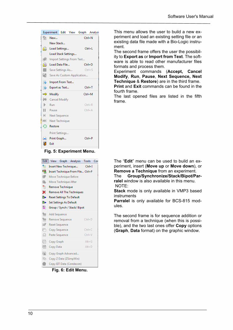
This menu allows the user to build a new ex-periment and load an existing setting file or an existing data file made with a Bio-Logic instru-ment. The second frame offers the user the possibil-ity to Export as or Import from Text. The soft-ware is able to read other manufacturer files formats and process them. Experiment commands (Accept, Cancel Modify, Run, Pause, Next Sequence, Next Technique & Restore) are in the third frame. Print and Exit commands can be found in the fourth frame. The last opened files are listed in the fifth frame.
Fig. 6: Edit Menu.
The “Edit” menu can be used to build an ex-periment, insert (Move up or Move down), or Remove a Technique from an experiment. The Group/Synchronize/Stack/Bipot/Par-ralel window is also available in this menu. NOTE: Stack mode is only available in VMP3 based instruments Parralel is only available for BCS-815 mod-ules. The second frame is for sequence addition or removal from a technique (when this is possi-ble), and the two last ones offer Copy options (Graph, Data format) on the graphic window.
Software User's Manual
11
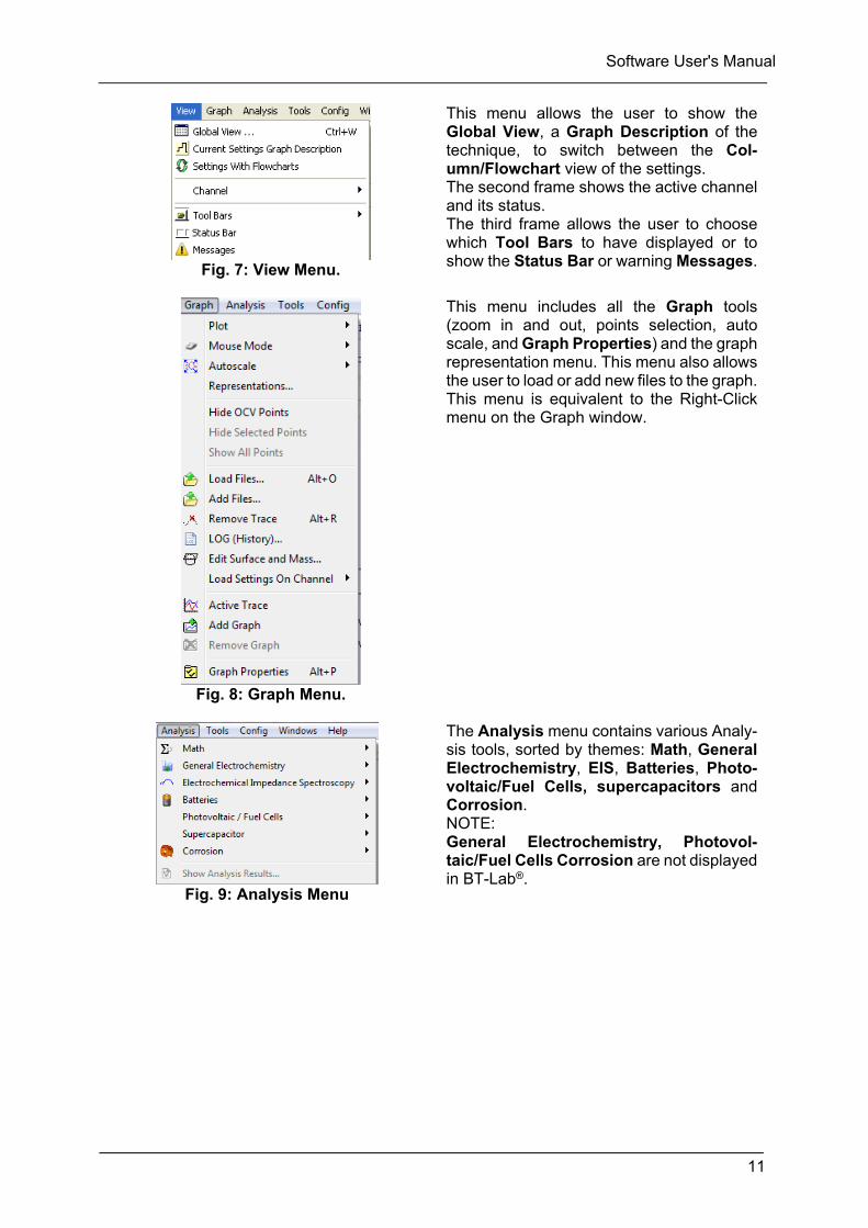
Fig. 7: View Menu.
This menu allows the user to show the Global View, a Graph Description of the technique, to switch between the Col-umn/Flowchart view of the settings. The second frame shows the active channel and its status. The third frame allows the user to choose which Tool Bars to have displayed or to show the Status Bar or warning Messages.
Fig. 8: Graph Menu.
This menu includes all the Graph tools (zoom in and out, points selection, auto scale, and Graph Properties) and the graph representation menu. This menu also allows the user to load or add new files to the graph. This menu is equivalent to the Right-Click menu on the Graph window.
Fig. 9: Analysis Menu
The Analysis menu contains various Analy-sis tools, sorted by themes: Math, General Electrochemistry, EIS, Batteries, Photo-voltaic/Fuel Cells, supercapacitors and Corrosion. NOTE: General Electrochemistry, Photovol-taic/Fuel Cells Corrosion are not displayed in BT-Lab®.
Software User's Manual
12
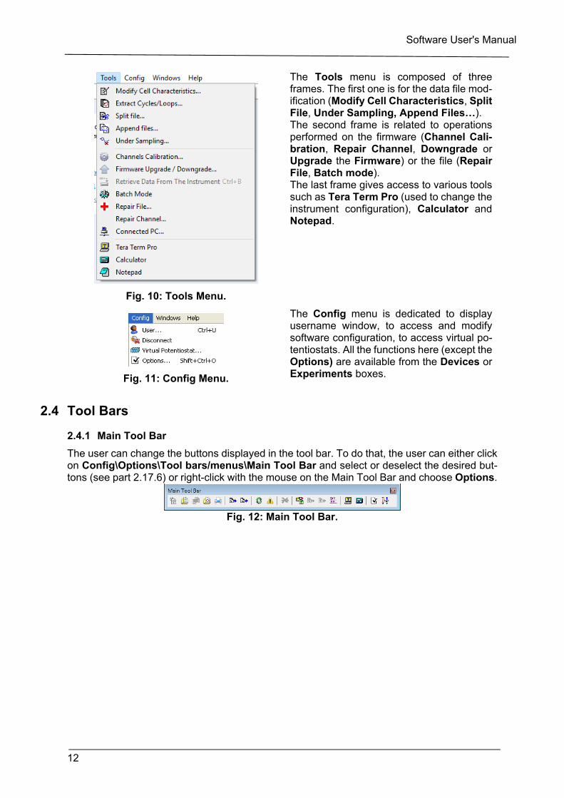
Fig. 10: Tools Menu.
The Tools menu is composed of three frames. The first one is for the data file mod-ification (Modify Cell Characteristics, Split File, Under Sampling, Append Files…). The second frame is related to operations performed on the firmware (Channel Cali-bration, Repair Channel, Downgrade or Upgrade the Firmware) or the file (Repair File, Batch mode). The last frame gives access to various tools such as Tera Term Pro (used to change the instrument configuration), Calculator and Notepad.
Fig. 11: Config Menu.
The Config menu is dedicated to display username window, to access and modify software configuration, to access virtual po-tentiostats. All the functions here (except the Options) are available from the Devices or Experiments boxes.
2.4 Tool Bars
2.4.1 Main Tool Bar
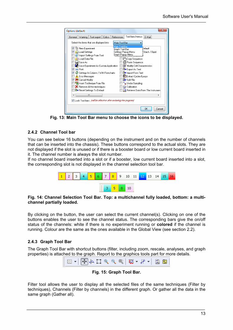
The user can change the buttons displayed in the tool bar. To do that, the user can either click on Config\Options\Tool bars/menus\Main Tool Bar and select or deselect the desired but-tons (see part 2.17.6) or right-click with the mouse on the Main Tool Bar and choose Options.
Fig. 12: Main Tool Bar.
Software User's Manual
13
Fig. 13: Main Tool Bar menu to choose the icons to be displayed.
2.4.2 Channel Tool bar
You can see below 16 buttons (depending on the instrument and on the number of channels that can be inserted into the chassis). These buttons correspond to the actual slots. They are not displayed if the slot is unused or if there is a booster board or low current board inserted in it. The channel number is always the slot number. If no channel board inserted into a slot or if a booster, low current board inserted into a slot, the corresponding slot is not displayed in the channel selection tool bar.
Fig. 14: Channel Selection Tool Bar. Top: a multichannel fully loaded, bottom: a multi-channel partially loaded.
By clicking on the button, the user can select the current channel(s). Clicking on one of the buttons enables the user to see the channel status. The corresponding bars give the on/off status of the channels: white if there is no experiment running or colored if the channel is running. Colour are the same as the ones available in the Global View (see section 2.2).
2.4.3 Graph Tool Bar
The Graph Tool Bar with shortcut buttons (filter, including zoom, rescale, analyses, and graph properties) is attached to the graph. Report to the graphics tools part for more details.
Fig. 15: Graph Tool Bar.
Filter tool allows the user to display all the selected files of the same techniques (Filter by techniques), Channels (Filter by channels) in the different graph. Or gather all the data in the same graph (Gather all).

Software User's Manual
14
Fig. 16: Graph Tool Bar.
Also attached to the Graph window is the Fast Graph Selection Tool Bar that can be used to rapidly plot certain variables and choose the cycles/loop to be displayed:
Fig. 17: Fast Graph Selection Tool Bar and cycle/loop filter.
2.4.4 Status Tool Bar
At the bottom of the main window, the Status Tool Bar can be seen.
The following information are displayed: the connected device the instrument’s IP (internet protocol) address if the instrument is connected to the com-
puter through an Ethernet connection or USB for an USB connection. For multichannel potentiostat/galvanostat or for measurements that require a fast sampling rate the use of the Ethernet connexion is strongly recommended.
the selected channel, a lock showing the Modify/Accept mode: “Read mode” or “Modify mode”, the remote status (received or disconnected). For VMP3 and VMP-300 based instru-
ments "Warm up autocalibration" is displayed when the instrument perform an autocal-ibration (usually after connecting the instrument to EC-Lab®)
the user name, the mouse coordinates on the graphic display, the data transfer rate in bit/s.
Fig. 18: Status Tool Bar for a VMP3 in EC-Lab®.
2.4.5 Current Values Tool Bar
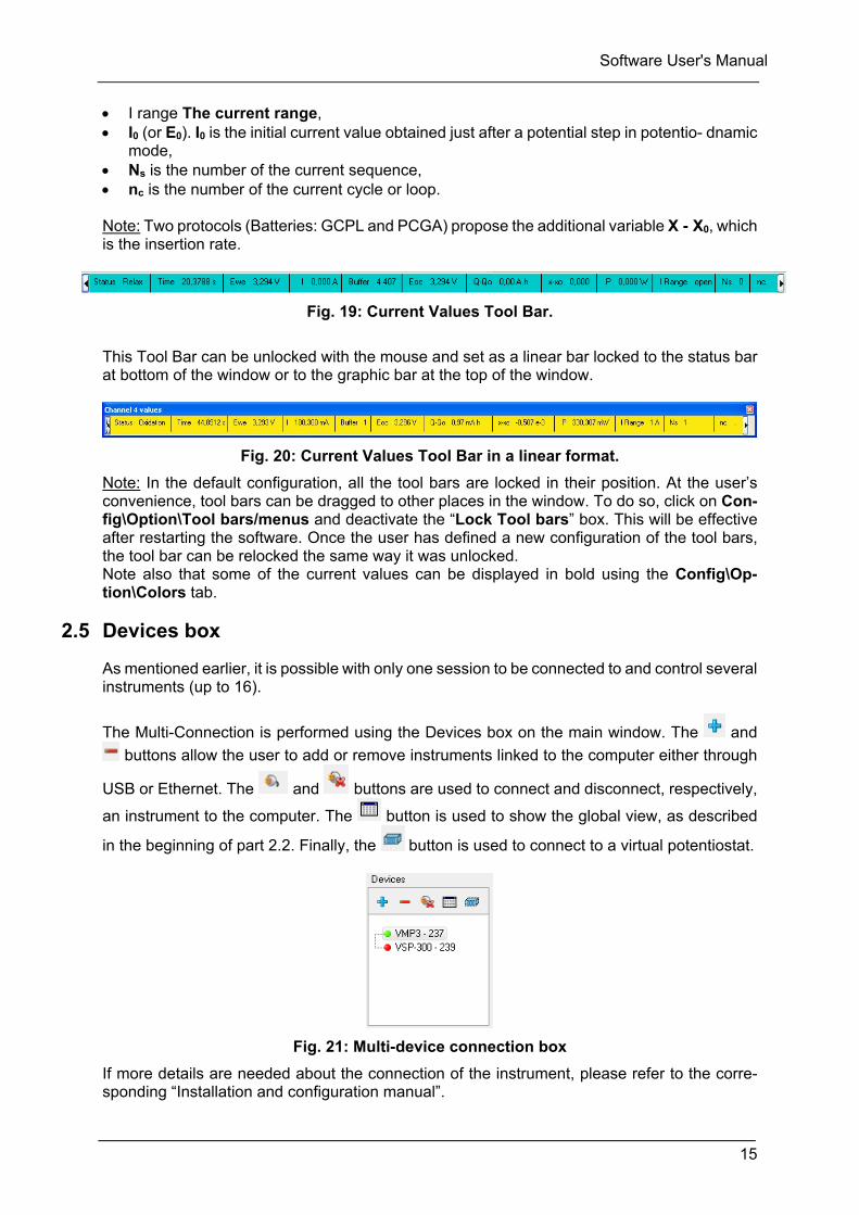
On the left side or at the bottom, the Tool Bar with the Current Values can be seen.
Status gives the nature of the running sequence: oxidation/charge, reduction/dis-charge, relax (open circuit, measuring the potential), paused or stopped. Buffer full will be displayed in the case where the instrument’s intermediate buffer is full (saturated net-work...),
Time, Ewe and Current are the time, the working electrode potential and the current from the beginning of the experiment,
Buffer indicates the buffer filling level Eoc is the potential value reached at the end of the previous open circuit period, Q - Q0 is the total charge since the beginning of the experiment,
Software User's Manual
15
I range The current range, I0 (or E0). I0 is the initial current value obtained just after a potential step in potentio- dnamic
mode, Ns is the number of the current sequence, nc is the number of the current cycle or loop. Note: Two protocols (Batteries: GCPL and PCGA) propose the additional variable X - X0, which is the insertion rate.
Fig. 19: Current Values Tool Bar.
This Tool Bar can be unlocked with the mouse and set as a linear bar locked to the status bar at bottom of the window or to the graphic bar at the top of the window.
Fig. 20: Current Values Tool Bar in a linear format.
Note: In the default configuration, all the tool bars are locked in their position. At the user’s convenience, tool bars can be dragged to other places in the window. To do so, click on Con-fig\Option\Tool bars/menus and deactivate the “Lock Tool bars” box. This will be effective after restarting the software. Once the user has defined a new configuration of the tool bars, the tool bar can be relocked the same way it was unlocked. Note also that some of the current values can be displayed in bold using the Config\Op-tion\Colors tab.
2.5 Devices box
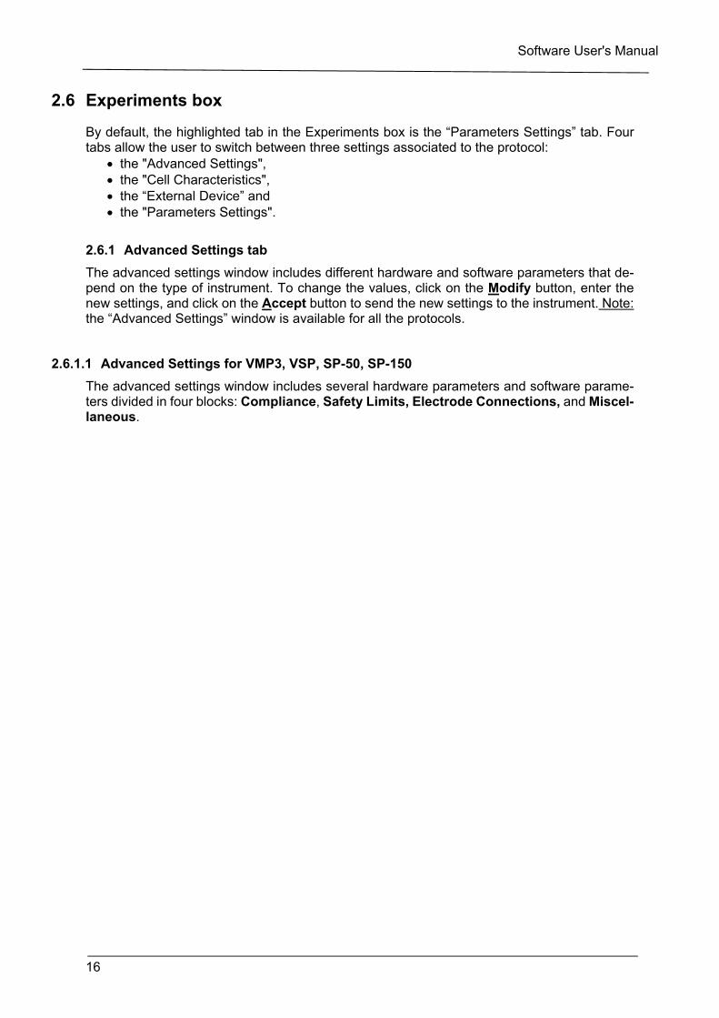
As mentioned earlier, it is possible with only one session to be connected to and control several instruments (up to 16).
The Multi-Connection is performed using the Devices box on the main window. The and
buttons allow the user to add or remove instruments linked to the computer either through
USB or Ethernet. The and buttons are used to connect and disconnect, respectively,
an instrument to the computer. The button is used to show the global view, as described
in the beginning of part 2.2. Finally, the button is used to connect to a virtual potentiostat.
Fig. 21: Multi-device connection box
If more details are needed about the connection of the instrument, please refer to the corre-sponding “Installation and configuration manual”.
Software User's Manual
16
2.6 Experiments box
By default, the highlighted tab in the Experiments box is the “Parameters Settings” tab. Four tabs allow the user to switch between three settings associated to the protocol:
the "Advanced Settings", the "Cell Characteristics", the “External Device” and the "Parameters Settings".
2.6.1 Advanced Settings tab
The advanced settings window includes different hardware and software parameters that de-pend on the type of instrument. To change the values, click on the Modify button, enter the new settings, and click on the Accept button to send the new settings to the instrument. Note: the “Advanced Settings” window is available for all the protocols.
2.6.1.1 Advanced Settings for VMP3, VSP, SP-50, SP-150
The advanced settings window includes several hardware parameters and software parame-ters divided in four blocks: Compliance, Safety Limits, Electrode Connections, and Miscel-laneous.
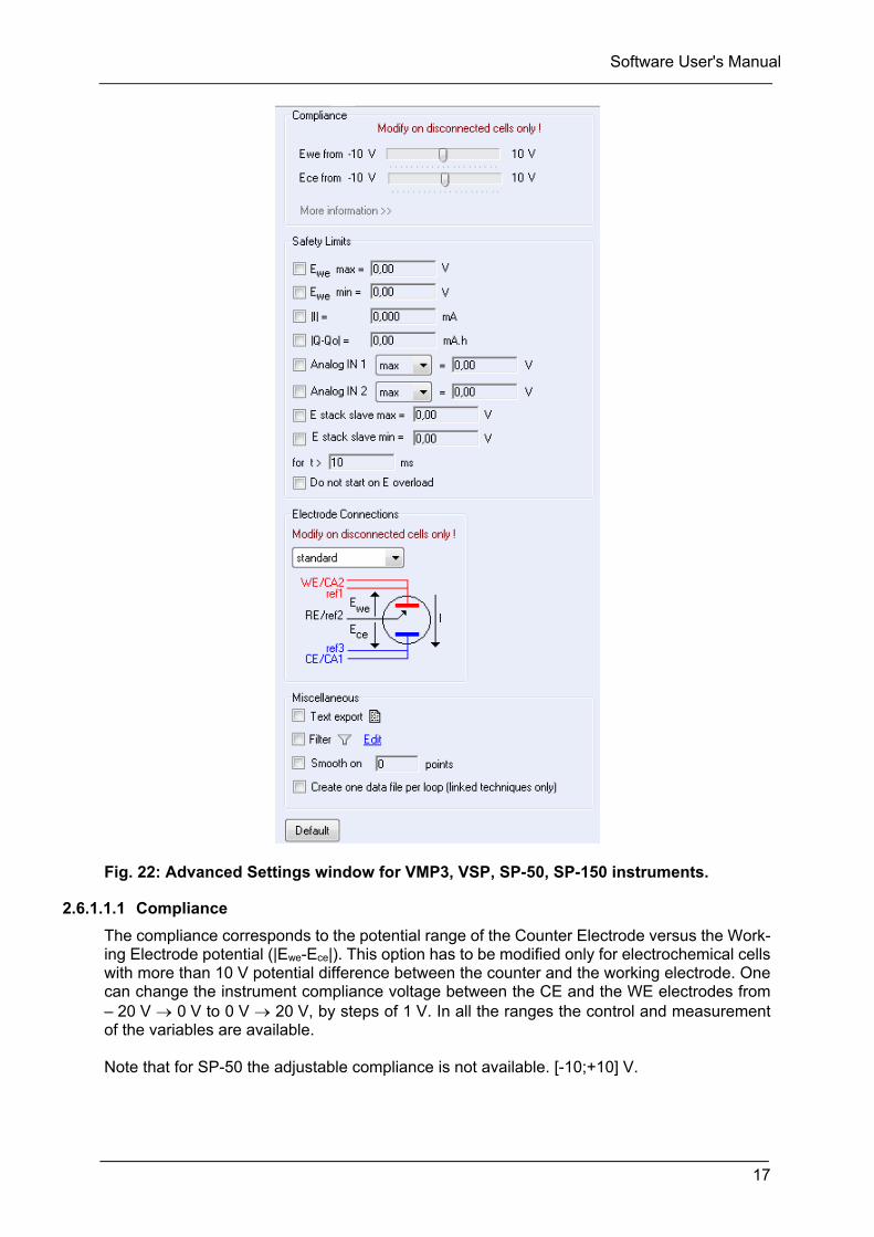
Software User's Manual
17
Fig. 22: Advanced Settings window for VMP3, VSP, SP-50, SP-150 instruments.
2.6.1.1.1 Compliance
The compliance corresponds to the potential range of the Counter Electrode versus the Work-ing Electrode potential (|Ewe-Ece|). This option has to be modified only for electrochemical cells with more than 10 V potential difference between the counter and the working electrode. One can change the instrument compliance voltage between the CE and the WE electrodes from – 20 V 0 V to 0 V 20 V, by steps of 1 V. In all the ranges the control and measurement of the variables are available. Note that for SP-50 the adjustable compliance is not available. [-10;+10] V.
Software User's Manual
18
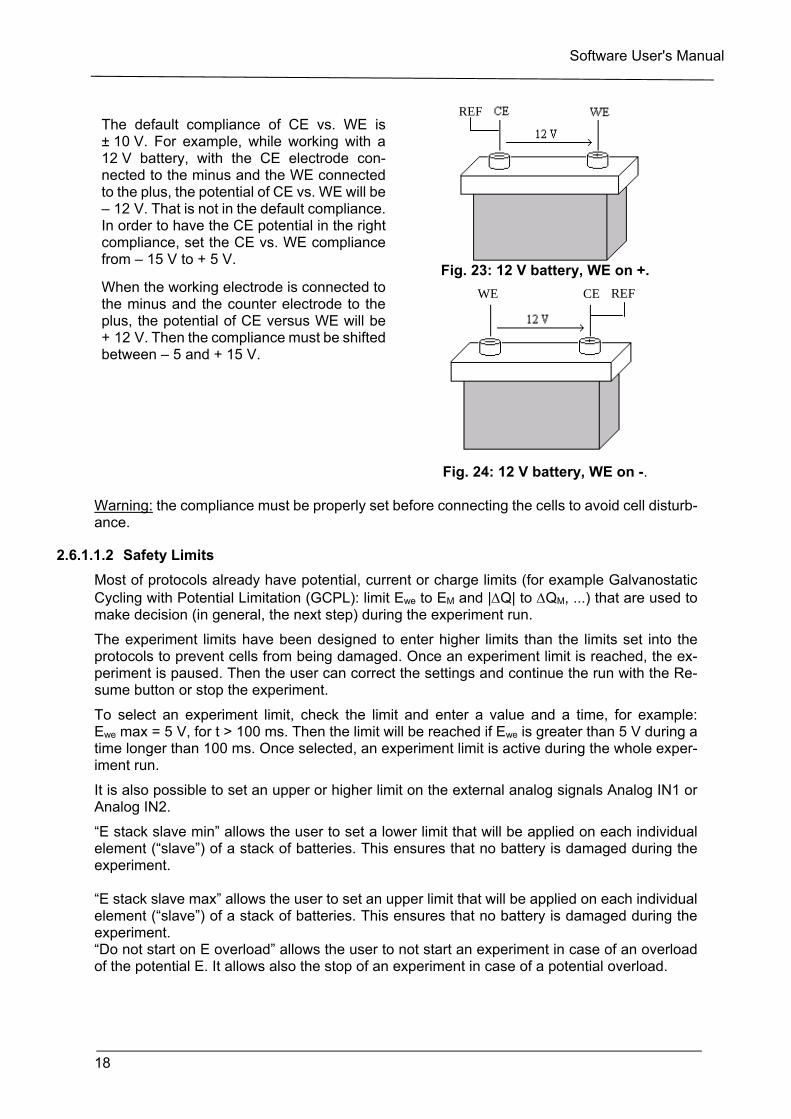
The default compliance of CE vs. WE is ± 10 V. For example, while working with a 12 V battery, with the CE electrode con-nected to the minus and the WE connected to the plus, the potential of CE vs. WE will be – 12 V. That is not in the default compliance. In order to have the CE potential in the right compliance, set the CE vs. WE compliance from – 15 V to + 5 V.
REF
Fig. 23: 12 V battery, WE on +.
When the working electrode is connected to the minus and the counter electrode to the plus, the potential of CE versus WE will be + 12 V. Then the compliance must be shifted between – 5 and + 15 V.
REF WE CE
Fig. 24: 12 V battery, WE on -. Warning: the compliance must be properly set before connecting the cells to avoid cell disturb-ance.
2.6.1.1.2 Safety Limits
Most of protocols already have potential, current or charge limits (for example Galvanostatic Cycling with Potential Limitation (GCPL): limit Ewe to EM and |Q| to QM, ...) that are used to make decision (in general, the next step) during the experiment run.
The experiment limits have been designed to enter higher limits than the limits set into the protocols to prevent cells from being damaged. Once an experiment limit is reached, the ex-periment is paused. Then the user can correct the settings and continue the run with the Re-sume button or stop the experiment.
To select an experiment limit, check the limit and enter a value and a time, for example: Ewe max = 5 V, for t > 100 ms. Then the limit will be reached if Ewe is greater than 5 V during a time longer than 100 ms. Once selected, an experiment limit is active during the whole exper-iment run.
It is also possible to set an upper or higher limit on the external analog signals Analog IN1 or Analog IN2.
“E stack slave min” allows the user to set a lower limit that will be applied on each individual element (“slave”) of a stack of batteries. This ensures that no battery is damaged during the experiment. “E stack slave max” allows the user to set an upper limit that will be applied on each individual element (“slave”) of a stack of batteries. This ensures that no battery is damaged during the experiment. “Do not start on E overload” allows the user to not start an experiment in case of an overload of the potential E. It allows also the stop of an experiment in case of a potential overload.
Software User's Manual
19
Warning: the safety limits cannot be modified during the experiment run and must be set be-fore.
2.6.1.1.3 Electrode Connections
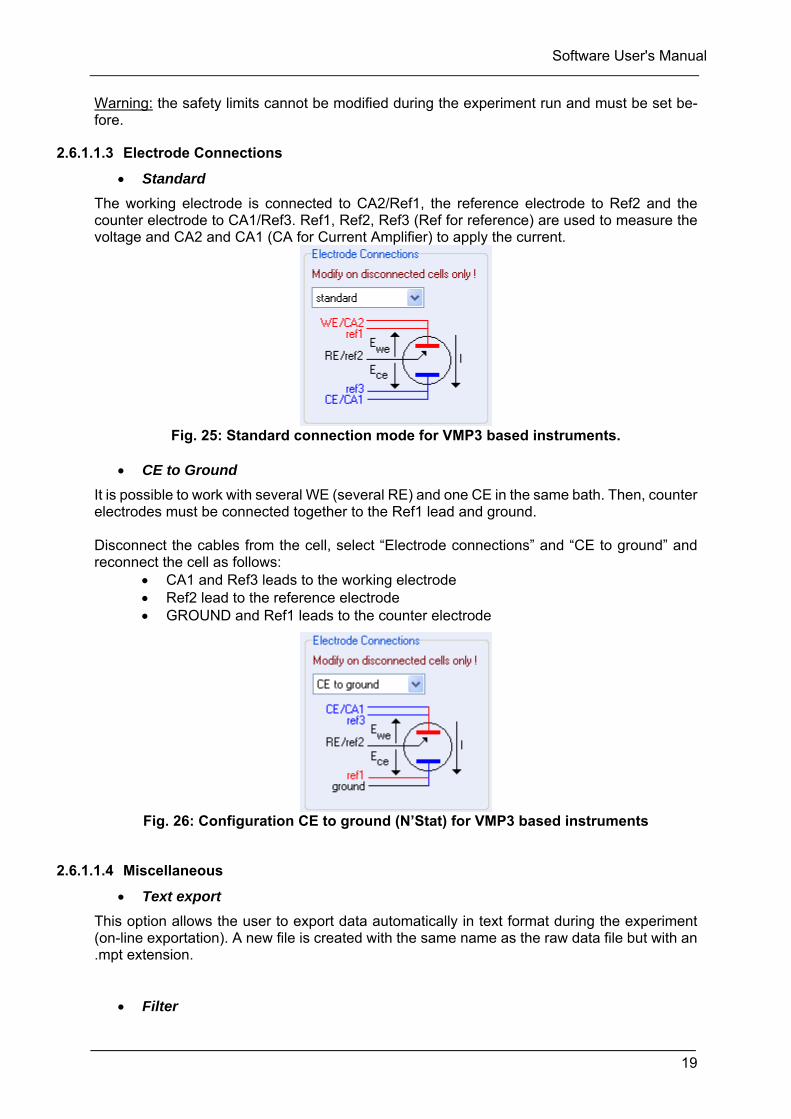
Standard
The working electrode is connected to CA2/Ref1, the reference electrode to Ref2 and the counter electrode to CA1/Ref3. Ref1, Ref2, Ref3 (Ref for reference) are used to measure the voltage and CA2 and CA1 (CA for Current Amplifier) to apply the current.
Fig. 25: Standard connection mode for VMP3 based instruments.
CE to Ground
It is possible to work with several WE (several RE) and one CE in the same bath. Then, counter electrodes must be connected together to the Ref1 lead and ground. Disconnect the cables from the cell, select “Electrode connections” and “CE to ground” and reconnect the cell as follows:
CA1 and Ref3 leads to the working electrode Ref2 lead to the reference electrode GROUND and Ref1 leads to the counter electrode
Fig. 26: Configuration CE to ground (N’Stat) for VMP3 based instruments
2.6.1.1.4 Miscellaneous
Text export
This option allows the user to export data automatically in text format during the experiment (on-line exportation). A new file is created with the same name as the raw data file but with an .mpt extension.
Filter
Software User's Manual
20
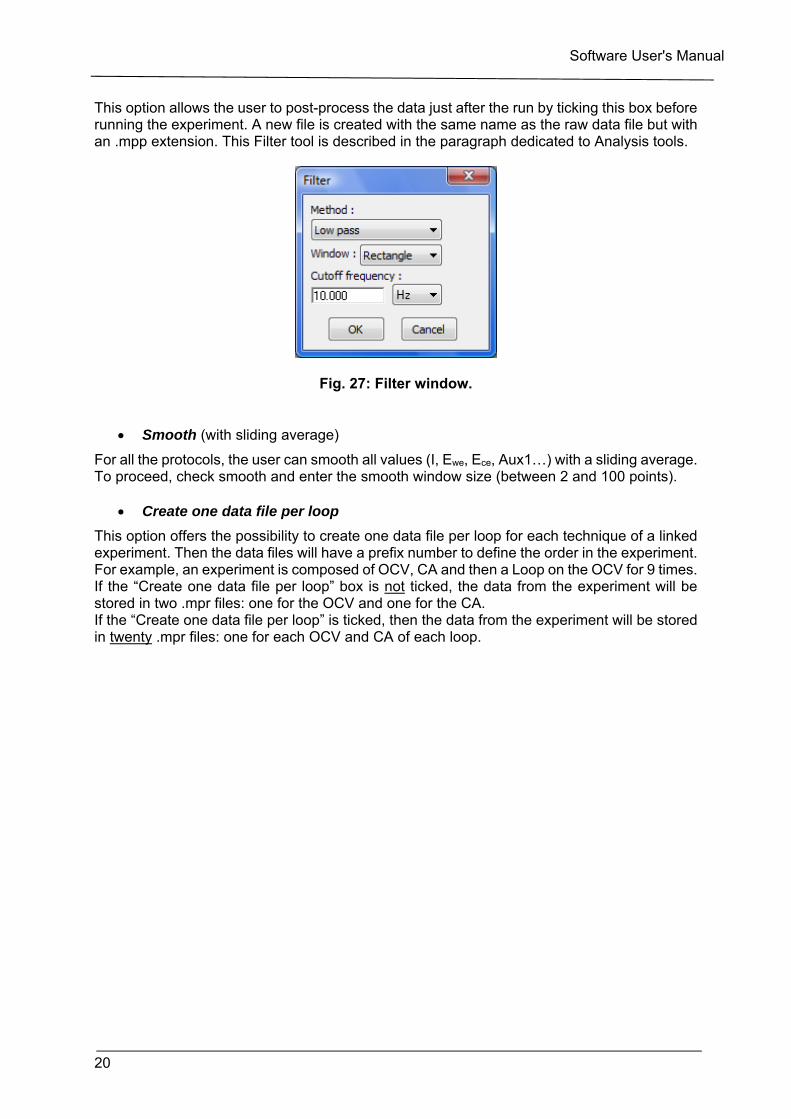
This option allows the user to post-process the data just after the run by ticking this box before running the experiment. A new file is created with the same name as the raw data file but with an .mpp extension. This Filter tool is described in the paragraph dedicated to Analysis tools.
Fig. 27: Filter window.
Smooth (with sliding average)
For all the protocols, the user can smooth all values (I, Ewe, Ece, Aux1…) with a sliding average. To proceed, check smooth and enter the smooth window size (between 2 and 100 points).
Create one data file per loop
This option offers the possibility to create one data file per loop for each technique of a linked experiment. Then the data files will have a prefix number to define the order in the experiment. For example, an experiment is composed of OCV, CA and then a Loop on the OCV for 9 times. If the “Create one data file per loop” box is not ticked, the data from the experiment will be stored in two .mpr files: one for the OCV and one for the CA. If the “Create one data file per loop” is ticked, then the data from the experiment will be stored in twenty .mpr files: one for each OCV and CA of each loop.
Software User's Manual
21
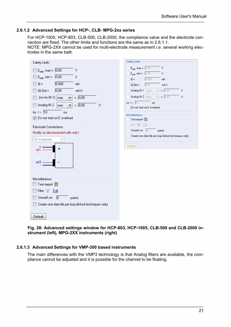
2.6.1.2 Advanced Settings for HCP-, CLB- MPG-2xx series
For HCP-1005, HCP-803, CLB-500, CLB-2000, the compliance value and the electrode con-nection are fixed. The other limits and functions are the same as in 2.6.1.1. NOTE: MPG-2XX cannot be used for multi-electrode measurement i.e. several working elec-trodes in the same bath
Fig. 28: Advanced settings window for HCP-803, HCP-1005, CLB-500 and CLB-2000 in-strument (left), MPG-2XX instruments (right)
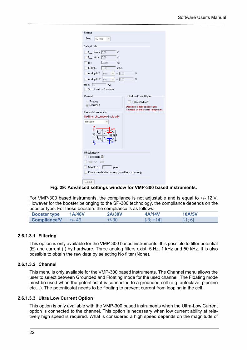
2.6.1.3 Advanced Settings for VMP-300 based instruments
The main differences with the VMP3 technology is that Analog filters are available, the com-pliance cannot be adjusted and it is possible for the channel to be floating.
Software User's Manual
22
Fig. 29: Advanced settings window for VMP-300 based instruments.
For VMP-300 based instruments, the compliance is not adjustable and is equal to +/- 12 V. However for the booster belonging to the SP-300 technology, the compliance depends on the booster type. For these boosters the compliance is as follows: Booster type 1A/48V 2A/30V 4A/14V 10A/5V Compliance/V +/- 49 +/-30 [-3; +14] [-1; 6]
2.6.1.3.1 Filtering
This option is only available for the VMP-300 based instruments. It is possible to filter potential (E) and current (I) by hardware. Three analog filters exist: 5 Hz, 1 kHz and 50 kHz. It is also possible to obtain the raw data by selecting No filter (None).
2.6.1.3.2 Channel
This menu is only available for the VMP-300 based instruments. The Channel menu allows the user to select between Grounded and Floating mode for the used channel. The Floating mode must be used when the potentiostat is connected to a grounded cell (e.g. autoclave, pipeline etc…). The potentiostat needs to be floating to prevent current from looping in the cell.
2.6.1.3.3 Ultra Low Current Option
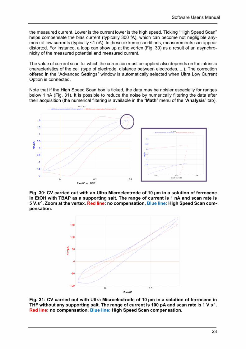
This option is only available with the VMP-300 based instruments when the Ultra-Low Current option is connected to the channel. This option is necessary when low current ability at rela-tively high speed is required. What is considered a high speed depends on the magnitude of
Software User's Manual
23
the measured current. Lower is the current lower is the high speed. Ticking “High Speed Scan” helps compensate the bias current (typically 300 fA), which can become not negligible any-more at low currents (typically <1 nA). In these extreme conditions, measurements can appear distorted. For instance, a loop can show up at the vertex (Fig. 30) as a result of an asynchro-nicity of the measured potential and measured current. The value of current scan for which the correction must be applied also depends on the intrinsic characteristics of the cell (type of electrode, distance between electrodes, ...). The correction offered in the “Advanced Settings” window is automatically selected when Ultra Low Current Option is connected. Note that if the High Speed Scan box is ticked, the data may be noisier especially for ranges below 1 nA (Fig. 31). It is possible to reduce the noise by numerically filtering the data after their acquisition (the numerical filtering is available in the “Math” menu of the “Analysis” tab).
Fig. 30: CV carried out with an Ultra Microelectrode of 10 µm in a solution of ferrocene in EtOH with TBAP as a supporting salt. The range of current is 1 nA and scan rate is 5 V.s-1. Zoom at the vertex. Red line: no compensation, Blue line: High Speed Scan com-pensation.
Fig. 31: CV carried out with Ultra Microelectrode of 10 µm in a solution of ferrocene in THF without any supporting salt. The range of current is 100 pA and scan rate is 1 V.s-1. Red line: no compensation, Blue line: High Speed Scan compensation.
Ewe/V
0.50
<I>
/pA
150
100
50
0
-50
-100
<I> vs . Ew e
UME_5Vs_sans compensation_1nA.mpr, cycle 3 # UME_5Vs_avec compensation_1nA.mpr, cycle 3
Ewe/V vs. SCE
0.40.20
<I>
/nA
2
1.5
1
0.5
0
-0.5
-1
-1.5
-2
<I> vs . Ew e
UME_5Vs_sans compensation_1nA.mpr, cycle 3 # UME_5Vs_avec compensation_1nA.mpr, cycle 3
Ewe/V vs. SCE
0.40.390.38
<I>
/nA
2.3
2.25
2.2
2.15
2.1
2.05
2
Software User's Manual
24
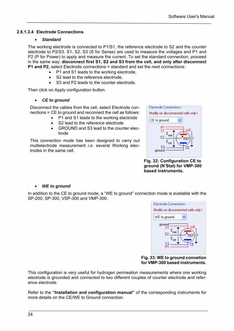
2.6.1.3.4 Electrode Connections
Standard
The working electrode is connected to P1/S1, the reference electrode to S2 and the counter electrode to P2/S3. S1, S2, S3 (S for Sense) are used to measure the voltages and P1 and P2 (P for Power) to apply and measure the current. To set the standard connection, proceed in the same way: disconnect first S1, S2 and S3 from the cell, and only after disconnect P1 and P2, select Electrode connections = standard and set the next connections:
P1 and S1 leads to the working electrode, S2 lead to the reference electrode, S3 and P2 leads to the counter electrode.
Then click on Apply configuration button.
CE to ground
Disconnect the cables from the cell, select Electrode con-nections = CE to ground and reconnect the cell as follows:
P1 and S1 leads to the working electrode S2 lead to the reference electrode GROUND and S3 lead to the counter elec-
trode
This connection mode has been designed to carry out multielectrode measurement i.e. several Working elec-trodes in the same cell.
Fig. 32: Configuration CE to ground (N’Stat) for VMP-300 based instruments.
WE to ground
In addition to the CE to ground mode, a “WE to ground” connection mode is available with the SP-200, SP-300, VSP-300 and VMP-300.
Fig. 33: WE to ground connetion for VMP-300 based instruments.
This configuration is very useful for hydrogen permeation measurements where one working electrode is grounded and connected to two different couples of counter electrode and refer-ence electrode. Refer to the “Installation and configuration manual” of the corresponding instruments for more details on the CE/WE to Ground connection.
Software User's Manual
25
Warning: it is important to disconnect the electrodes from the cell, before changing the elec-trode connection, because of the difference between the leads assignment, the OCV may not be properly applied. Note: with CE to ground connection, CE vs. WE compliance is set to 12 V. The CE to ground option is not available with the ZRA protocol (Zero Resistance Ammeter).
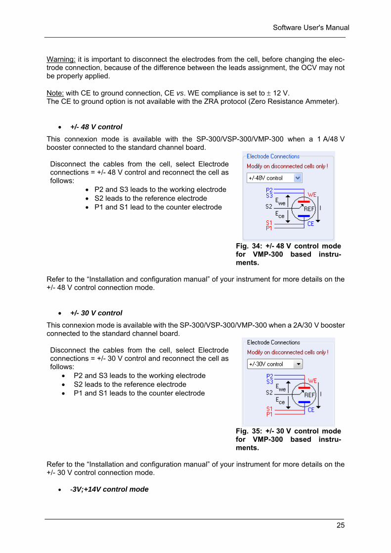
+/- 48 V control
This connexion mode is available with the SP-300/VSP-300/VMP-300 when a 1 A/48 V booster connected to the standard channel board. Disconnect the cables from the cell, select Electrode connections = +/- 48 V control and reconnect the cell as follows:
P2 and S3 leads to the working electrode S2 leads to the reference electrode P1 and S1 lead to the counter electrode
Fig. 34: +/- 48 V control mode for VMP-300 based instru-ments.
Refer to the “Installation and configuration manual” of your instrument for more details on the +/- 48 V control connection mode.
+/- 30 V control
This connexion mode is available with the SP-300/VSP-300/VMP-300 when a 2A/30 V booster connected to the standard channel board. Disconnect the cables from the cell, select Electrode connections = +/- 30 V control and reconnect the cell as follows:
P2 and S3 leads to the working electrode S2 leads to the reference electrode P1 and S1 leads to the counter electrode
Fig. 35: +/- 30 V control mode for VMP-300 based instru-ments.
Refer to the “Installation and configuration manual” of your instrument for more details on the +/- 30 V control connection mode.
-3V;+14V control mode
Software User's Manual
26
The +14V;-3V is two-electrodes connexion mode available with the SP-240 and with SP-300/VSP-300/VMP-300 when a 4A/14 V booster connected to the standard channel board. Disconnect the cables from the cell, select Electrode connections = -3V,+14 V control and reconnect the cell as follows: - P1, S1 and S2 leads to the working electrode - S3 and P2 leads to the counter electrode P.S: The impedance techniques are not available with -3V;+14V control mode.
Fig. 36:-3V;+14V control mode for VMP-300 based instru-ments.
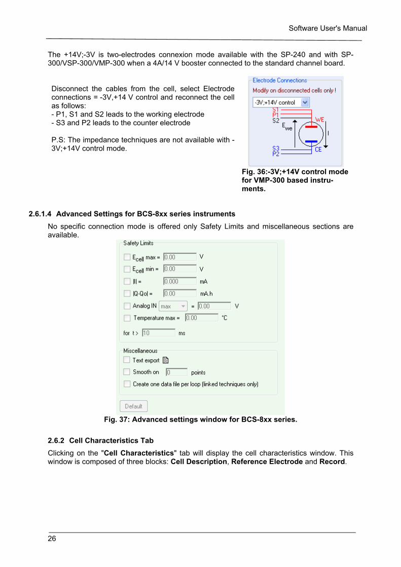
2.6.1.4 Advanced Settings for BCS-8xx series instruments
No specific connection mode is offered only Safety Limits and miscellaneous sections are available.
Fig. 37: Advanced settings window for BCS-8xx series.
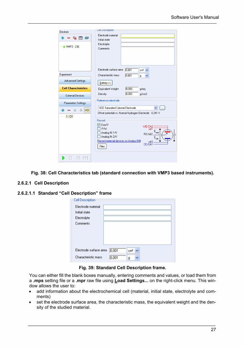
2.6.2 Cell Characteristics Tab
Clicking on the "Cell Characteristics" tab will display the cell characteristics window. This window is composed of three blocks: Cell Description, Reference Electrode and Record.
Software User's Manual
27
Fig. 38: Cell Characteristics tab (standard connection with VMP3 based instruments).
2.6.2.1 Cell Description
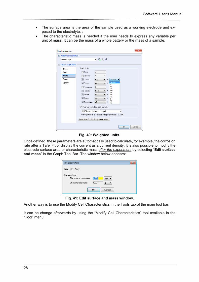
2.6.2.1.1 Standard “Cell Description” frame
Fig. 39: Standard Cell Description frame.
You can either fill the blank boxes manually, entering comments and values, or load them from a .mps setting file or a .mpr raw file using Load Settings... on the right-click menu. This win-dow allows the user to: add information about the electrochemical cell (material, initial state, electrolyte and com-
ments) set the electrode surface area, the characteristic mass, the equivalent weight and the den-
sity of the studied material.
Software User's Manual
28
The surface area is the area of the sample used as a working electrode and ex-posed to the electrolyte. :
The characteristic mass is needed if the user needs to express any variable per unit of mass. It can be the mass of a whole battery or the mass of a sample.
Fig. 40: Weighted units.
Once defined, these parameters are automatically used to calculate, for example, the corrosion rate after a Tafel Fit or display the current as a current density. It is also possible to modify the electrode surface area or characteristic mass after the experiment by selecting “Edit surface and mass” in the Graph Tool Bar. The window below appears:
Fig. 41: Edit surface and mass window.
Another way is to use the Modify Cell Characteristics in the Tools tab of the main tool bar. It can be change afterwards by using the “Modify Cell Characteristics” tool available in the “Tool” menu.
Software User's Manual
29
Fig. 42: Modify Cell Characteristics window.
For battery and corrosion applications, additional variable can be added. These applications are discussed hereafter.
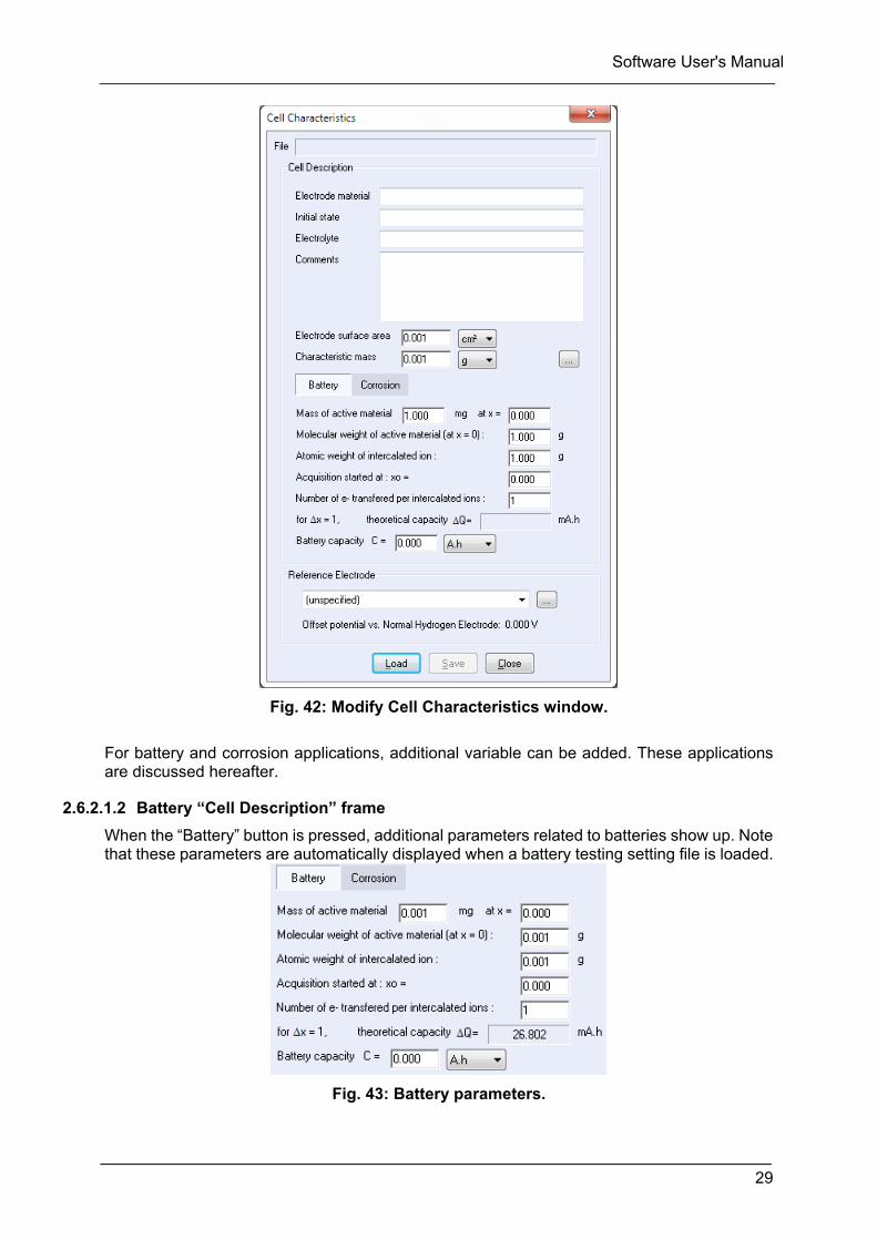
2.6.2.1.2 Battery “Cell Description” frame
When the “Battery” button is pressed, additional parameters related to batteries show up. Note that these parameters are automatically displayed when a battery testing setting file is loaded.
Fig. 43: Battery parameters.

Software User's Manual
30
This window allows the user to enter the physical characteristics corresponding to the interca-lation material. This makes on-line monitoring of the redox processes possible in terms of nor-malized units.
The mass of active material in the cell has to be set with a given insertion coefficient xmass in the compound of interest (for example xmass = 1 for LiCoO2). These two parameters mass and xmass are actually related to the battery itself. This mass is dif-ferent from the characteristic mass. It is only used to calculate the insertion rate x and not the massic variables: (I, Q, P, C, Energy)/unit of mass
The molecular weight of the active material is the molecular weight of the active mate-rial subtracted by the atomic weight of the intercalated ion. The atomic weight of the intercalated ion is set in a separate box. For example, for LiCoO2, the molecular weight of CoO2 is 90.93 g.mol-1 and the atomic weight of the intercalated Lithium Li+ is 6.94 g.mol-1.
The initial insertion rate xo. ne is the number of electrons transferred per mole of intercalated ion.
An intermediate variable Xf is calculated using the following formula:
Mass is in mg, Molecular weight and the atomic weight are in g/mol, this is why mass needs to be multiplied by 0.001, F is equal to 26801 mA.h/mol. Xf quantifies the change of insertion coefficient of the considered ion when a charge of 1 mA.h is passed through the cell (or deintercalated when a discharge of -1 mA.h is passed). The charge needed to increase Xf of 1 is given in the window: “for x=1, Q= 26802 mA.h”. The variable x, which is the insertion coefficient of the inserted ion (or stoichiometry of the inserted ion in the concerned compound) resulting from the charge, is calculated using the following formula:
x = xo + Xf (Q-Qo)
x is the sum of xo the initial insertion coefficient and Xf the change of insertion coefficient during the charge (or deintercalated during the discharge) Q-Qo. Qo is the initial state of charge of the battery and is calculated using xo.
Finally, it is possible to enter the capacity C of the battery in A.h or mA.h. The capacity of the battery is the total charge that can be passed in the battery. A capacity of 3.2 A.h means that the fully charged battery will be totally discharged if a current of -3.2 A is applied during 1 hour. In the techniques dedicated to batteries and especially the GCPL techniques and Modulo Bat technique (MB), it is possible to define the charge or discharge current as a function of the capacity. For instance, using a battery of 3.2 A.h, if the charge is set at C/2, it means that the battery will be charged with a current of 1.6 A. The time of the charge is defined elsewhere in the technique (see “Software Techniques and Applications” manual). NOTE: this is not the values set in the theoretical capacity which is used. Several templates are available with different chemistries and battery sizes are available. Cus-tomized templates can be created and saved.
Software User's Manual
31
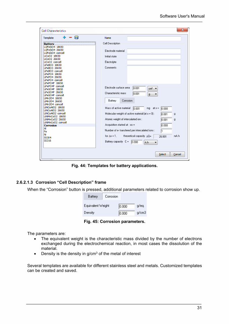
Fig. 44: Templates for battery applications.
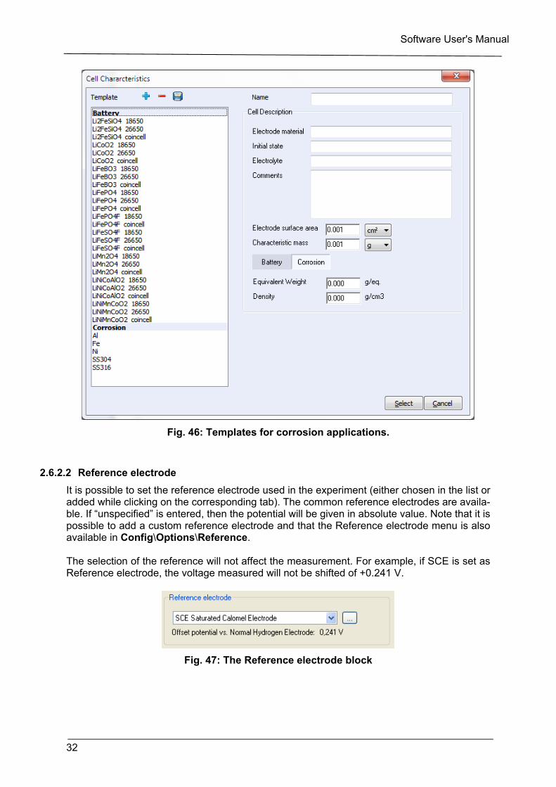
2.6.2.1.3 Corrosion “Cell Description” frame
When the “Corrosion” button is pressed, additional parameters related to corrosion show up.
Fig. 45: Corrosion parameters.
The parameters are:
The equivalent weight is the characteristic mass divided by the number of electrons exchanged during the electrochemical reaction, in most cases the dissolution of the material.
Density is the density in g/cm3 of the metal of interest
Several templates are available for different stainless steel and metals. Customized templates can be created and saved.
Software User's Manual
32
Fig. 46: Templates for corrosion applications.
2.6.2.2 Reference electrode
It is possible to set the reference electrode used in the experiment (either chosen in the list or added while clicking on the corresponding tab). The common reference electrodes are availa-ble. If “unspecified” is entered, then the potential will be given in absolute value. Note that it is possible to add a custom reference electrode and that the Reference electrode menu is also available in Config\Options\Reference. The selection of the reference will not affect the measurement. For example, if SCE is set as Reference electrode, the voltage measured will not be shifted of +0.241 V.
Fig. 47: The Reference electrode block
Software User's Manual
33
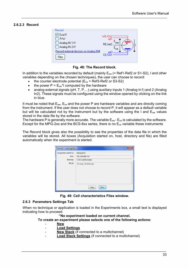
2.6.2.3 Record
Fig. 48: The Record block.
In addition to the variables recorded by default (mainly Ewe (= Ref1-Ref2 or S1-S2), I and other variables depending on the chosen techniques), the user can choose to record:
the counter electrode potential (Ece = Ref3-Ref2 or S3-S2) the power P = Ewe*I computed by the hardware analog external signals (pH, T, P,...) using auxiliary inputs 1 (Analog In1) and 2 (Analog
In2). These signals must be configured using the window opened by clicking on the link in blue.
It must be noted that Ewe, Ece and the power P are hardware variables and are directly coming from the instrument. If the user does not choose to record P, it will appear as a default variable but will be calculated not by the instrument but by the software using the I and Ewe values stored in the data file by the software. The hardware P is generally more accurate. The variable Ewe - Ece is calculated by the software. Except for the MPG-2xx and the BCS-8xx series, there is no Ece variable these instruments The Record block gives also the possibility to see the properties of the data file in which the variables will be stored. All boxes (Acquisition started on, host, directory and file) are filled automatically when the experiment is started.
Fig. 49: Cell characteristics Files window.
2.6.3 Parameters Settings Tab
When no technique or application is loaded in the Experiments box, a small text is displayed indicating how to proceed:
“No experiment loaded on current channel. To create an experiment please selects one of the following actions:
- New - Load Settings - New Stack (if connected to a multichannel) - Load Stack Settings (if connected to a multichannel)

Software User's Manual
34
The column will contain the techniques of a linked experiment. The settings of each technique will be available by clicking on the icon of the technique.
The “Turn to OCV between techniques” option offers the possibility to add an OCV period between linked techniques. This OCV period allows the instrument to change its current ranging. It lasts 50 ms.
Fig. 50: Top row in the Parameters Settings window.
NOTE: If this period is followed by a technique in which the voltage is defined vs. Eoc, the OCV determined during this period will not be used.
The button is available to show the graph describing the technique and its variables.
2.6.3.1 Right-click on the “Parameters Settings” tab
The software contains a context menu: Right-click on the main window to display all the commands available on the mouse
right-click. Commands on the mouse right-click depend on the displayed window. Other com-
mands are available with the mouse right-click on the graphic display.
Most of the commands are available with the right-click. They are separated into 6 frames. The first frame concerns the available setting tabs, the second one is for the experiment from building to printing. The third frame is for the modification of an experiment (actions on techniques) and the creation of linked experiments. The fourth one is dedicated to sequences (addition, re-moval) and the fifth one to the controls during the run. The sixth and seventh frames are additional functions de-scribed above and the last frame is a di-rect access to the Options tab.
Fig. 51: Mouse right-click on the main win-dow.
Software User's Manual
35
2.6.3.2 Selecting a technique
First select a channel on the channel bar. There are three different ways to load a new exper-iment.
1- Click on the “New Experiment” button . 2- Click on the blue “New” link on the parameter settings window. 3- The user can also click on the right button of the mouse and select “New Experiment”
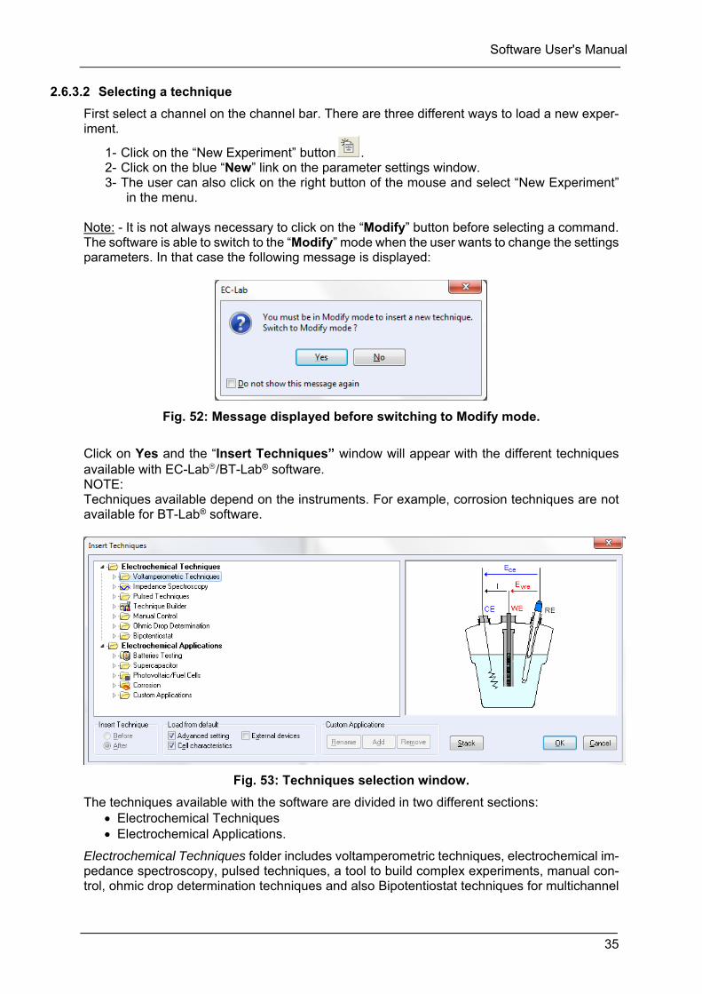
in the menu. Note: - It is not always necessary to click on the “Modify” button before selecting a command. The software is able to switch to the “Modify” mode when the user wants to change the settings parameters. In that case the following message is displayed:
Fig. 52: Message displayed before switching to Modify mode.
Click on Yes and the “Insert Techniques” window will appear with the different techniques available with EC-Lab/BT-Lab® software. NOTE: Techniques available depend on the instruments. For example, corrosion techniques are not available for BT-Lab® software.
Fig. 53: Techniques selection window.
The techniques available with the software are divided in two different sections: Electrochemical Techniques Electrochemical Applications.
Electrochemical Techniques folder includes voltamperometric techniques, electrochemical im-pedance spectroscopy, pulsed techniques, a tool to build complex experiments, manual con-trol, ohmic drop determination techniques and also Bipotentiostat techniques for multichannel
Software User's Manual
36
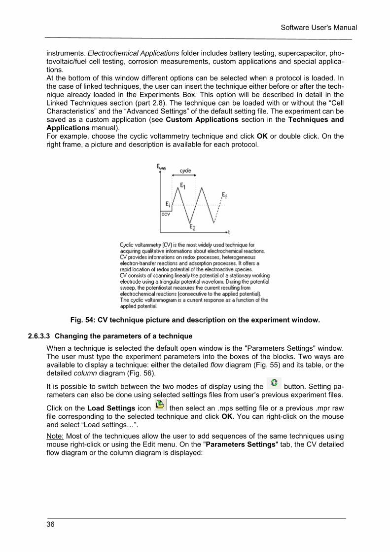
instruments. Electrochemical Applications folder includes battery testing, supercapacitor, pho-tovoltaic/fuel cell testing, corrosion measurements, custom applications and special applica-tions. At the bottom of this window different options can be selected when a protocol is loaded. In the case of linked techniques, the user can insert the technique either before or after the tech-nique already loaded in the Experiments Box. This option will be described in detail in the Linked Techniques section (part 2.8). The technique can be loaded with or without the “Cell Characteristics” and the “Advanced Settings” of the default setting file. The experiment can be saved as a custom application (see Custom Applications section in the Techniques and Applications manual). For example, choose the cyclic voltammetry technique and click OK or double click. On the right frame, a picture and description is available for each protocol.
Fig. 54: CV technique picture and description on the experiment window.
2.6.3.3 Changing the parameters of a technique
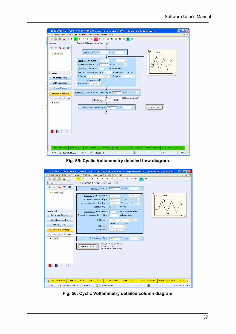
When a technique is selected the default open window is the "Parameters Settings" window. The user must type the experiment parameters into the boxes of the blocks. Two ways are available to display a technique: either the detailed flow diagram (Fig. 55) and its table, or the detailed column diagram (Fig. 56).
It is possible to switch between the two modes of display using the button. Setting pa-rameters can also be done using selected settings files from user’s previous experiment files.
Click on the Load Settings icon then select an .mps setting file or a previous .mpr raw file corresponding to the selected technique and click OK. You can right-click on the mouse and select “Load settings…”.
Note: Most of the techniques allow the user to add sequences of the same techniques using mouse right-click or using the Edit menu. On the "Parameters Settings" tab, the CV detailed flow diagram or the column diagram is displayed:
Software User's Manual
37
Fig. 55: Cyclic Voltammetry detailed flow diagram.
Fig. 56: Cyclic Voltammetry detailed column diagram.
Software User's Manual
38
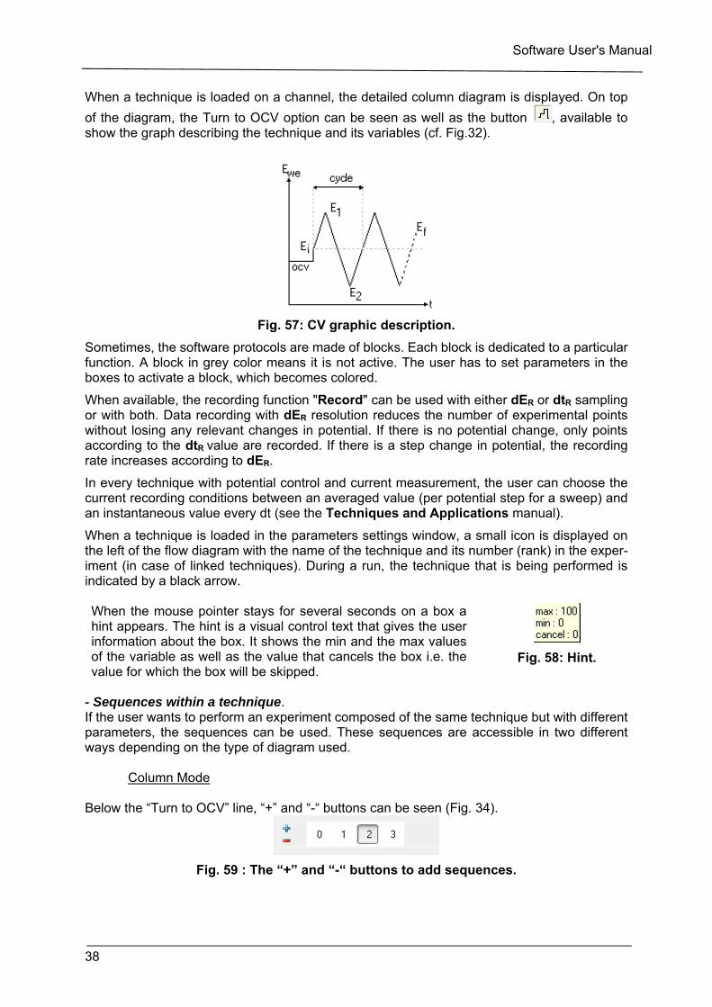
When a technique is loaded on a channel, the detailed column diagram is displayed. On top
of the diagram, the Turn to OCV option can be seen as well as the button , available to show the graph describing the technique and its variables (cf. Fig.32).
Fig. 57: CV graphic description.
Sometimes, the software protocols are made of blocks. Each block is dedicated to a particular function. A block in grey color means it is not active. The user has to set parameters in the boxes to activate a block, which becomes colored.
When available, the recording function "Record" can be used with either dER or dtR sampling or with both. Data recording with dER resolution reduces the number of experimental points without losing any relevant changes in potential. If there is no potential change, only points according to the dtR value are recorded. If there is a step change in potential, the recording rate increases according to dER.
In every technique with potential control and current measurement, the user can choose the current recording conditions between an averaged value (per potential step for a sweep) and an instantaneous value every dt (see the Techniques and Applications manual).
When a technique is loaded in the parameters settings window, a small icon is displayed on the left of the flow diagram with the name of the technique and its number (rank) in the exper-iment (in case of linked techniques). During a run, the technique that is being performed is indicated by a black arrow.
When the mouse pointer stays for several seconds on a box a hint appears. The hint is a visual control text that gives the user information about the box. It shows the min and the max values of the variable as well as the value that cancels the box i.e. the value for which the box will be skipped.
Fig. 58: Hint.
- Sequences within a technique. If the user wants to perform an experiment composed of the same technique but with different parameters, the sequences can be used. These sequences are accessible in two different ways depending on the type of diagram used. Column Mode Below the “Turn to OCV” line, “+” and “-“ buttons can be seen (Fig. 34).
Fig. 59 : The “+” and “-“ buttons to add sequences.
Software User's Manual
39
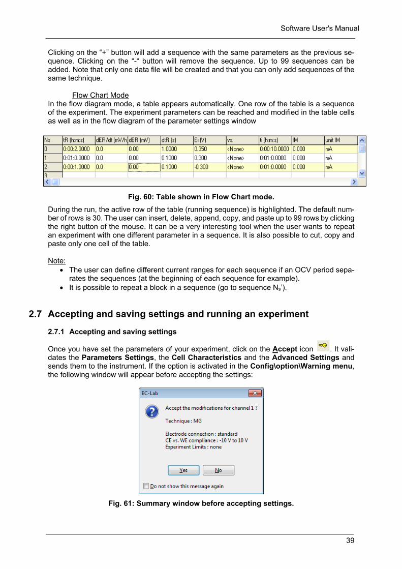
Clicking on the “+” button will add a sequence with the same parameters as the previous se-quence. Clicking on the “-“ button will remove the sequence. Up to 99 sequences can be added. Note that only one data file will be created and that you can only add sequences of the same technique. Flow Chart Mode In the flow diagram mode, a table appears automatically. One row of the table is a sequence of the experiment. The experiment parameters can be reached and modified in the table cells as well as in the flow diagram of the parameter settings window
Fig. 60: Table shown in Flow Chart mode.
During the run, the active row of the table (running sequence) is highlighted. The default num-ber of rows is 30. The user can insert, delete, append, copy, and paste up to 99 rows by clicking the right button of the mouse. It can be a very interesting tool when the user wants to repeat an experiment with one different parameter in a sequence. It is also possible to cut, copy and paste only one cell of the table. Note:
The user can define different current ranges for each sequence if an OCV period sepa-rates the sequences (at the beginning of each sequence for example).
It is possible to repeat a block in a sequence (go to sequence Ns’).
2.7 Accepting and saving settings and running an experiment
2.7.1 Accepting and saving settings
Once you have set the parameters of your experiment, click on the Accept icon . It vali-dates the Parameters Settings, the Cell Characteristics and the Advanced Settings and sends them to the instrument. If the option is activated in the Config\option\Warning menu, the following window will appear before accepting the settings:
Fig. 61: Summary window before accepting settings.
Software User's Manual
40
This window summarizes several parameters of the experiment. Click on Yes to accept the settings and start the experiment. The settings can be set as default settings for the current technique. Right-click on the mouse and select “Set settings as Default”. The parameter set-tings can be saved as an *.mps file in Experiment\save as\ or right-click on Save Experi-
ment…, or click on .
2.7.2 Running an experiment
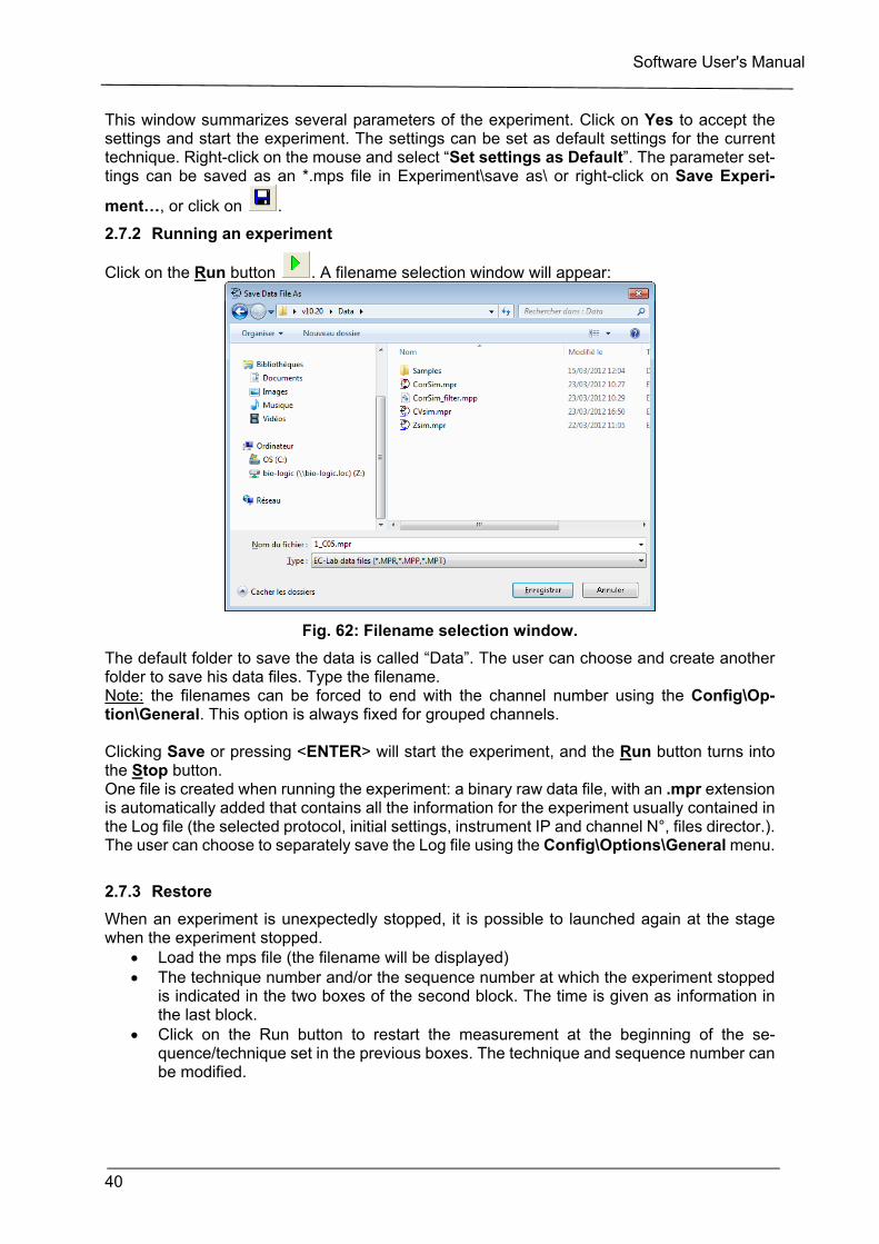
Click on the Run button . A filename selection window will appear:
Fig. 62: Filename selection window.
The default folder to save the data is called “Data”. The user can choose and create another folder to save his data files. Type the filename. Note: the filenames can be forced to end with the channel number using the Config\Op-tion\General. This option is always fixed for grouped channels. Clicking Save or pressing <ENTER> will start the experiment, and the Run button turns into the Stop button. One file is created when running the experiment: a binary raw data file, with an .mpr extension is automatically added that contains all the information for the experiment usually contained in the Log file (the selected protocol, initial settings, instrument IP and channel N°, files director.). The user can choose to separately save the Log file using the Config\Options\General menu.
2.7.3 Restore
When an experiment is unexpectedly stopped, it is possible to launched again at the stage when the experiment stopped.
Load the mps file (the filename will be displayed) The technique number and/or the sequence number at which the experiment stopped
is indicated in the two boxes of the second block. The time is given as information in the last block.
Click on the Run button to restart the measurement at the beginning of the se-quence/technique set in the previous boxes. The technique and sequence number can be modified.

Software User's Manual
41
Fig. 63: Restore function.
The restore function create a new mpr file. It is possible to append the two files by using the append files function available in the tool menu. The initial file is loaded in the File 1 box and the other file in the file 2 box. The location of the resulting file (mpr format) will be stored in the folder defined in the third box. The name of the resulting file will be “file 1_Append”. Click on Append to start the process.
Fig. 64: Append files function.
2.8 Linking techniques
2.8.1 Description and settings
It is possible to link different protocols within the same run. This allows the user to create and build complex experiments composed of up to 20 techniques. Once created, the linked exper-iment settings can be saved either as an .mps file or as a “Custom Application”. In the first case the settings can be loaded from the initial folder, and in the second case they appear in the applications and can be reloaded whenever necessary.
Software User's Manual
42
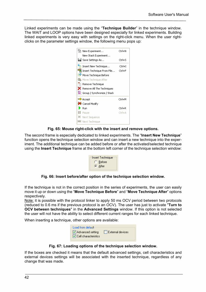
Linked experiments can be made using the “Technique Builder” in the technique window. The WAIT and LOOP options have been designed especially for linked experiments. Building linked experiments is very easy with settings on the right-click menu. When the user right-clicks on the parameter settings window, the following menu pops up:
Fig. 65: Mouse right-click with the insert and remove options.
The second frame is especially dedicated to linked experiments. The “Insert New Technique” function opens the technique selection window and can insert a new technique into the exper-iment. The additional technique can be added before or after the activated/selected technique using the Insert Technique frame at the bottom left corner of the technique selection window:
Fig. 66: Insert before/after option of the technique selection window.
If the technique is not in the correct position in the series of experiments, the user can easily move it up or down using the “Move Technique Before” and “Move Technique After” options respectively. Note: it is possible with the protocol linker to apply 50 ms OCV period between two protocols (reduced to 0.6 ms if the previous protocol is an OCV). The user has just to activate "Turn to OCV between techniques" in the Advanced Settings window. If this option is not selected the user will not have the ability to select different current ranges for each linked technique.
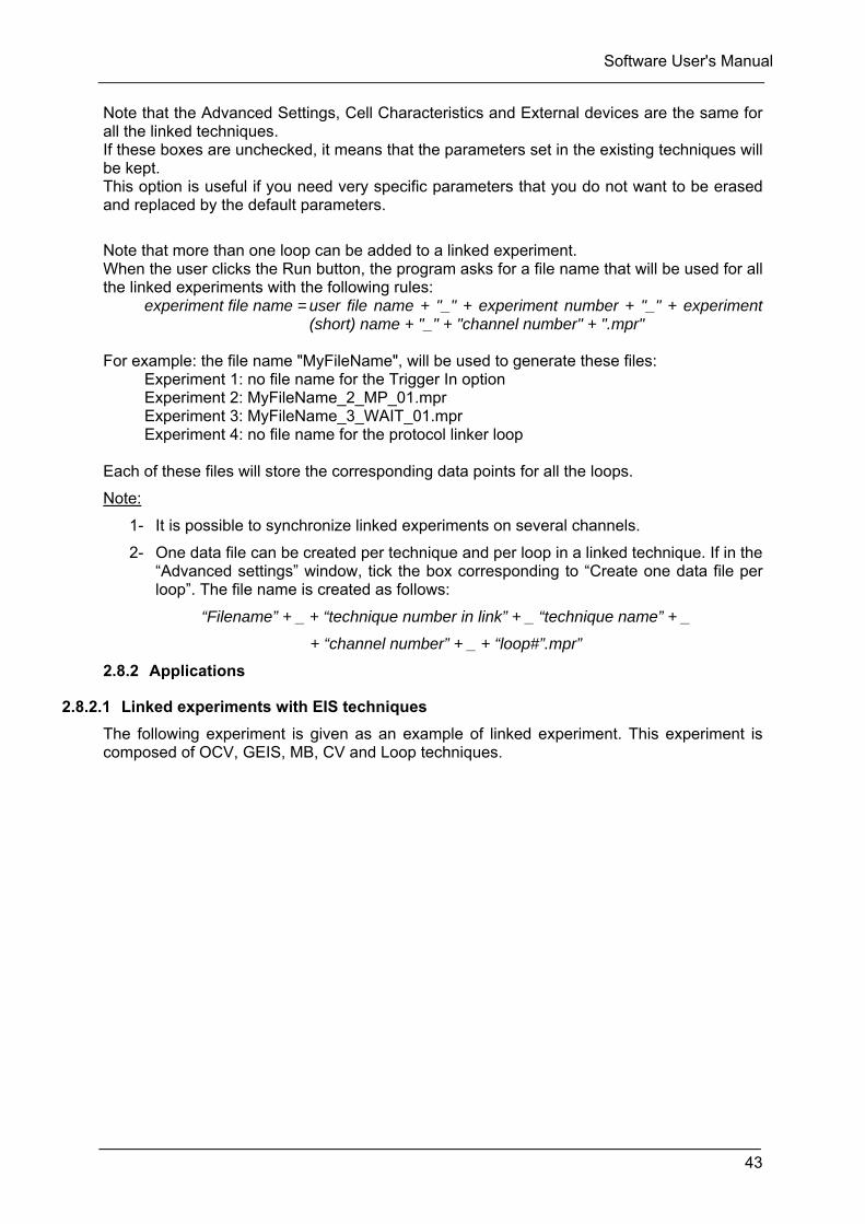
When inserting a technique, other options are available:
Fig. 67: Loading options of the technique selection window.
If the boxes are checked it means that the default advanced settings, cell characteristics and external devices settings will be associated with the inserted technique, regardless of any change that was made.
Software User's Manual
43
Note that the Advanced Settings, Cell Characteristics and External devices are the same for all the linked techniques. If these boxes are unchecked, it means that the parameters set in the existing techniques will be kept. This option is useful if you need very specific parameters that you do not want to be erased and replaced by the default parameters.
Note that more than one loop can be added to a linked experiment. When the user clicks the Run button, the program asks for a file name that will be used for all the linked experiments with the following rules:
experiment file name = user file name + "_" + experiment number + "_" + experiment (short) name + "_" + "channel number" + ".mpr"
For example: the file name "MyFileName", will be used to generate these files:
Experiment 1: no file name for the Trigger In option Experiment 2: MyFileName_2_MP_01.mpr Experiment 3: MyFileName_3_WAIT_01.mpr Experiment 4: no file name for the protocol linker loop
Each of these files will store the corresponding data points for all the loops.
Note:
1- It is possible to synchronize linked experiments on several channels.
2- One data file can be created per technique and per loop in a linked technique. If in the “Advanced settings” window, tick the box corresponding to “Create one data file per loop”. The file name is created as follows:
“Filename” + _ + “technique number in link” + _ “technique name” + _
+ “channel number” + _ + “loop#”.mpr”
2.8.2 Applications
2.8.2.1 Linked experiments with EIS techniques
The following experiment is given as an example of linked experiment. This experiment is composed of OCV, GEIS, MB, CV and Loop techniques.
Software User's Manual
44
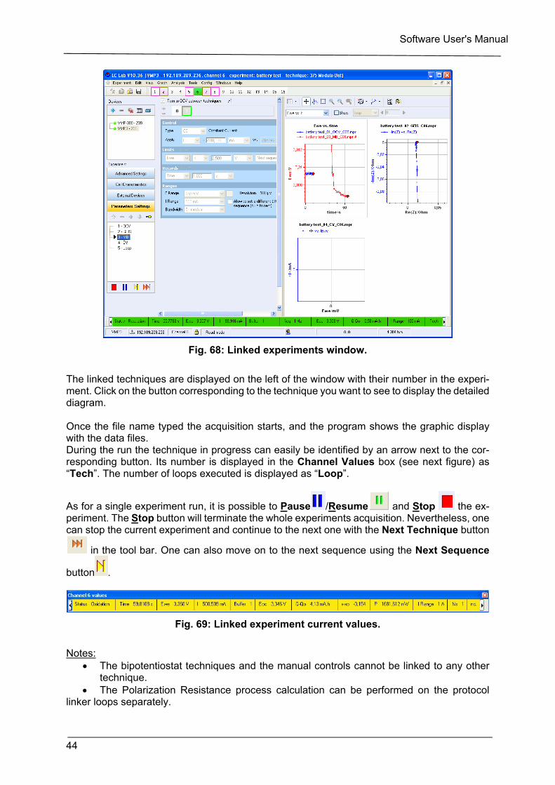
Fig. 68: Linked experiments window.
The linked techniques are displayed on the left of the window with their number in the experi-ment. Click on the button corresponding to the technique you want to see to display the detailed diagram. Once the file name typed the acquisition starts, and the program shows the graphic display with the data files. During the run the technique in progress can easily be identified by an arrow next to the cor-responding button. Its number is displayed in the Channel Values box (see next figure) as “Tech”. The number of loops executed is displayed as “Loop”.
As for a single experiment run, it is possible to Pause /Resume and Stop the ex-periment. The Stop button will terminate the whole experiments acquisition. Nevertheless, one can stop the current experiment and continue to the next one with the Next Technique button
in the tool bar. One can also move on to the next sequence using the Next Sequence
button .
Fig. 69: Linked experiment current values.
Notes:
The bipotentiostat techniques and the manual controls cannot be linked to any other technique.
The Polarization Resistance process calculation can be performed on the protocol linker loops separately.
Software User's Manual
45
Linked experiments settings can be saved with Experiment, Save As, or on the right-click menu with Save experiment… and reloaded with Experiment, Load settings... or with the right-click menu Load settings.... Linked experiments settings files are text files with the *.mps extension like the standard set-tings files.
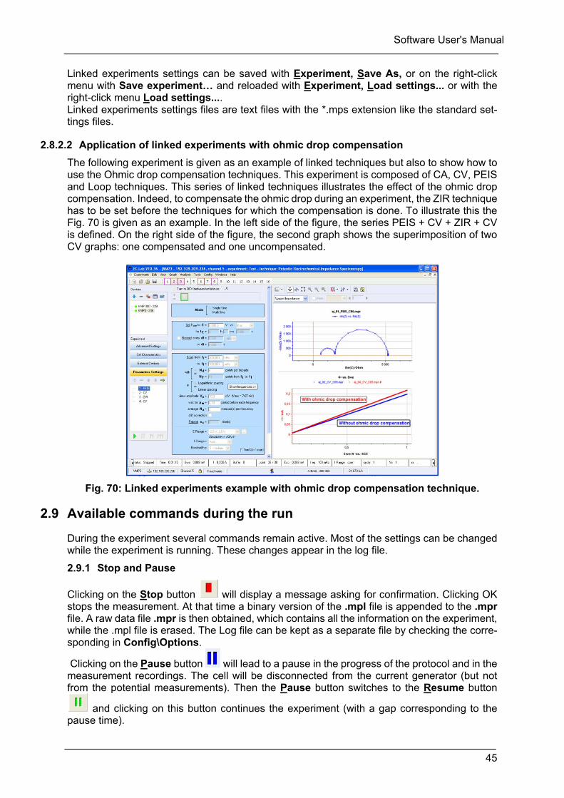
2.8.2.2 Application of linked experiments with ohmic drop compensation
The following experiment is given as an example of linked techniques but also to show how to use the Ohmic drop compensation techniques. This experiment is composed of CA, CV, PEIS and Loop techniques. This series of linked techniques illustrates the effect of the ohmic drop compensation. Indeed, to compensate the ohmic drop during an experiment, the ZIR technique has to be set before the techniques for which the compensation is done. To illustrate this the Fig. 70 is given as an example. In the left side of the figure, the series PEIS + CV + ZIR + CV is defined. On the right side of the figure, the second graph shows the superimposition of two CV graphs: one compensated and one uncompensated.
Fig. 70: Linked experiments example with ohmic drop compensation technique.
2.9 Available commands during the run
During the experiment several commands remain active. Most of the settings can be changed while the experiment is running. These changes appear in the log file.
2.9.1 Stop and Pause
Clicking on the Stop button will display a message asking for confirmation. Clicking OK stops the measurement. At that time a binary version of the .mpl file is appended to the .mpr file. A raw data file .mpr is then obtained, which contains all the information on the experiment, while the .mpl file is erased. The Log file can be kept as a separate file by checking the corre-sponding in Config\Options.
Clicking on the Pause button will lead to a pause in the progress of the protocol and in the measurement recordings. The cell will be disconnected from the current generator (but not from the potential measurements). Then the Pause button switches to the Resume button
and clicking on this button continues the experiment (with a gap corresponding to the pause time).
Software User's Manual
46
2.9.2 Next Technique/Next Sequence
It is possible during an experiment to move on to the Next Technique using the button
or to the Next Sequence using the button.
2.9.3 Modifying an experiment in progress
The Modify button enables the user to modify most of the parameter settings while the experiment is running.
The new set of parameters is sent to the instrument when clicking on the Accept button . It is taken into account within 200 µs for instruments of the VMP3 and VMP-300 based instru-ments and 2 ms for BT-Lab®. All information on the change, the time it was done, the new settings etc., is appended to the Log file (see section 3.2.6, page 79). Note that a warning message could appear before accepting the modification if this option is selected in Con-fig\Option\Warning. Among all the parameters, some of them cannot be modified on the fly such as I range E range and Bandwidth.
2.9.4 Repair channel
This tool allows a user to repair a channel board. To have repair channel window, click on Tools menu and then repair channel menu. The window below will be open. The window contains four blocks:
First block
Selection of the channel the user wants to repair. The user should not modify the connection mode (Ethernet or USB). In case of a multichannel instrument, it is recommended to select the channel to repair and then select the same channel number in the repair channel window.
Second block
This block allows user to lock the data transfer of the selected channel. In the case of a multichannel, because of a wrong recording parameter (most of time dE or dI) on one channel, many data points may be recorded and fill the buffer of the com board. The data transfer procedure is stuck to this specific channel and is much slower for the other chan-nels of the instrument. This tool allows user to block the data transfer of this channel, the data point of the other channel will be retrieved.
Third block
Allows the user to create a new file to store the coming data point. It is useful for example when the user moves an experiment file during the experiment. In that case, the user will have one file for the first part of the experiment and another one for data points which are not yet transferred to the PC (after the creation of the new file).
Fourth block
This will reset all the data point stored in the buffer of the communication board related to the selected channel. This tool has to be used if the tool of the second and the third block doesn’t work.
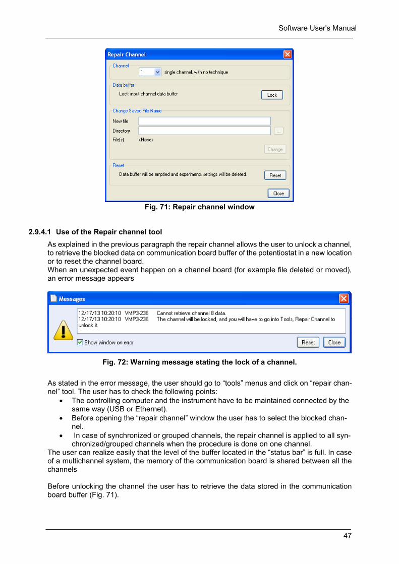
Software User's Manual
47
Fig. 71: Repair channel window
2.9.4.1 Use of the Repair channel tool
As explained in the previous paragraph the repair channel allows the user to unlock a channel, to retrieve the blocked data on communication board buffer of the potentiostat in a new location or to reset the channel board. When an unexpected event happen on a channel board (for example file deleted or moved), an error message appears
Fig. 72: Warning message stating the lock of a channel.
As stated in the error message, the user should go to “tools” menus and click on “repair chan-nel” tool. The user has to check the following points:
The controlling computer and the instrument have to be maintained connected by the same way (USB or Ethernet).
Before opening the “repair channel” window the user has to select the blocked chan-nel.
In case of synchronized or grouped channels, the repair channel is applied to all syn-chronized/grouped channels when the procedure is done on one channel.
The user can realize easily that the level of the buffer located in the “status bar” is full. In case of a multichannel system, the memory of the communication board is shared between all the channels Before unlocking the channel the user has to retrieve the data stored in the communication board buffer (Fig. 71).
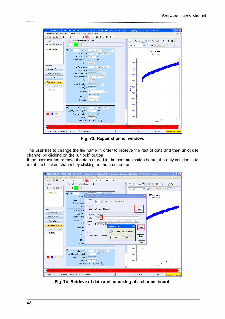
Software User's Manual
48
Fig. 73: Repair channel window.
The user has to change the file name in order to retrieve the rest of data and then unlock le channel by clicking on the “unlock” button. If the user cannot retrieve the data stored in the communication board, the only solution is to reset the blocked channel by clicking on the reset button.
Fig. 74: Retrieve of data and unlocking of a channel board.
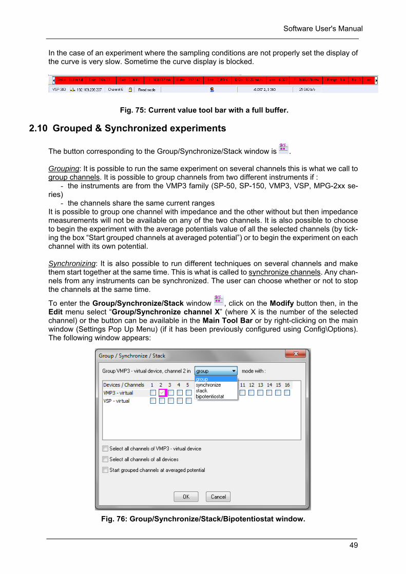
Software User's Manual
49
In the case of an experiment where the sampling conditions are not properly set the display of the curve is very slow. Sometime the curve display is blocked.
Fig. 75: Current value tool bar with a full buffer.
2.10 Grouped & Synchronized experiments
The button corresponding to the Group/Synchronize/Stack window is . Grouping: It is possible to run the same experiment on several channels this is what we call to group channels. It is possible to group channels from two different instruments if :
- the instruments are from the VMP3 family (SP-50, SP-150, VMP3, VSP, MPG-2xx se-ries)
- the channels share the same current ranges It is possible to group one channel with impedance and the other without but then impedance measurements will not be available on any of the two channels. It is also possible to choose to begin the experiment with the average potentials value of all the selected channels (by tick-ing the box “Start grouped channels at averaged potential”) or to begin the experiment on each channel with its own potential. Synchronizing: It is also possible to run different techniques on several channels and make them start together at the same time. This is what is called to synchronize channels. Any chan-nels from any instruments can be synchronized. The user can choose whether or not to stop the channels at the same time.
To enter the Group/Synchronize/Stack window , click on the Modify button then, in the Edit menu select “Group/Synchronize channel X” (where X is the number of the selected channel) or the button can be available in the Main Tool Bar or by right-clicking on the main window (Settings Pop Up Menu) (if it has been previously configured using Config\Options). The following window appears:
Fig. 76: Group/Synchronize/Stack/Bipotentiostat window.
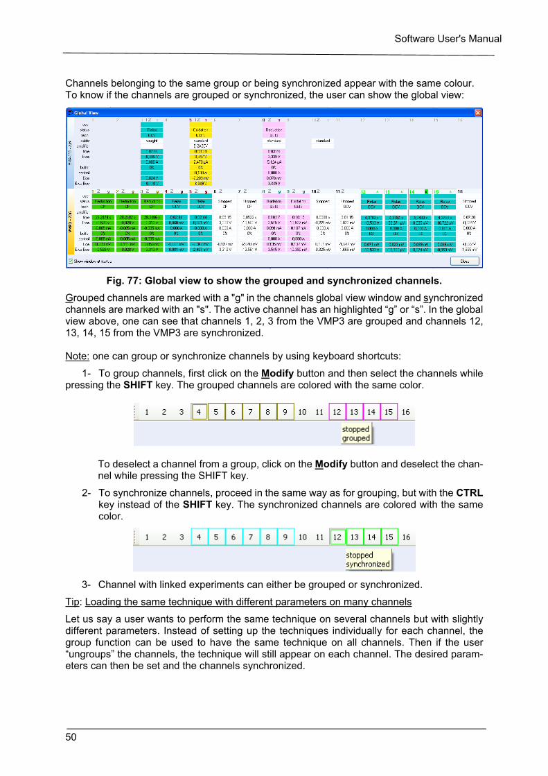
Software User's Manual
50
Channels belonging to the same group or being synchronized appear with the same colour. To know if the channels are grouped or synchronized, the user can show the global view:
Fig. 77: Global view to show the grouped and synchronized channels.
Grouped channels are marked with a "g" in the channels global view window and synchronized channels are marked with an "s". The active channel has an highlighted “g” or “s”. In the global view above, one can see that channels 1, 2, 3 from the VMP3 are grouped and channels 12, 13, 14, 15 from the VMP3 are synchronized. Note: one can group or synchronize channels by using keyboard shortcuts:
1- To group channels, first click on the Modify button and then select the channels while pressing the SHIFT key. The grouped channels are colored with the same color.
To deselect a channel from a group, click on the Modify button and deselect the chan-nel while pressing the SHIFT key.
2- To synchronize channels, proceed in the same way as for grouping, but with the CTRL key instead of the SHIFT key. The synchronized channels are colored with the same color.
3- Channel with linked experiments can either be grouped or synchronized.
Tip: Loading the same technique with different parameters on many channels
Let us say a user wants to perform the same technique on several channels but with slightly different parameters. Instead of setting up the techniques individually for each channel, the group function can be used to have the same technique on all channels. Then if the user “ungroups” the channels, the technique will still appear on each channel. The desired param-eters can then be set and the channels synchronized.
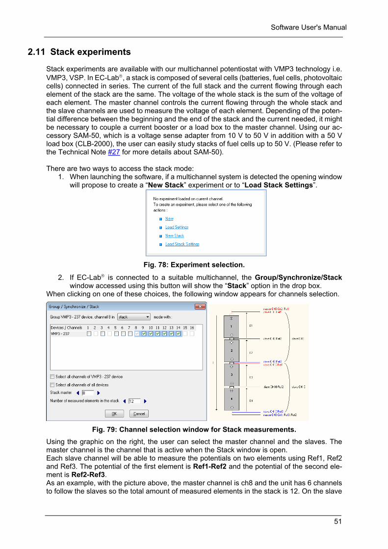
Software User's Manual
51
2.11 Stack experiments
Stack experiments are available with our multichannel potentiostat with VMP3 technology i.e. VMP3, VSP. In EC-Lab, a stack is composed of several cells (batteries, fuel cells, photovoltaic cells) connected in series. The current of the full stack and the current flowing through each element of the stack are the same. The voltage of the whole stack is the sum of the voltage of each element. The master channel controls the current flowing through the whole stack and the slave channels are used to measure the voltage of each element. Depending of the poten-tial difference between the beginning and the end of the stack and the current needed, it might be necessary to couple a current booster or a load box to the master channel. Using our ac-cessory SAM-50, which is a voltage sense adapter from 10 V to 50 V in addition with a 50 V load box (CLB-2000), the user can easily study stacks of fuel cells up to 50 V. (Please refer to the Technical Note #27 for more details about SAM-50). There are two ways to access the stack mode:
1. When launching the software, if a multichannel system is detected the opening window will propose to create a “New Stack” experiment or to “Load Stack Settings”.
Fig. 78: Experiment selection.
2. If EC-Lab is connected to a suitable multichannel, the Group/Synchronize/Stack window accessed using this button will show the “Stack” option in the drop box.
When clicking on one of these choices, the following window appears for channels selection.
Fig. 79: Channel selection window for Stack measurements.
Using the graphic on the right, the user can select the master channel and the slaves. The master channel is the channel that is active when the Stack window is open. Each slave channel will be able to measure the potentials on two elements using Ref1, Ref2 and Ref3. The potential of the first element is Ref1-Ref2 and the potential of the second ele-ment is Ref2-Ref3. As an example, with the picture above, the master channel is ch8 and the unit has 6 channels to follow the slaves so the total amount of measured elements in the stack is 12. On the slave
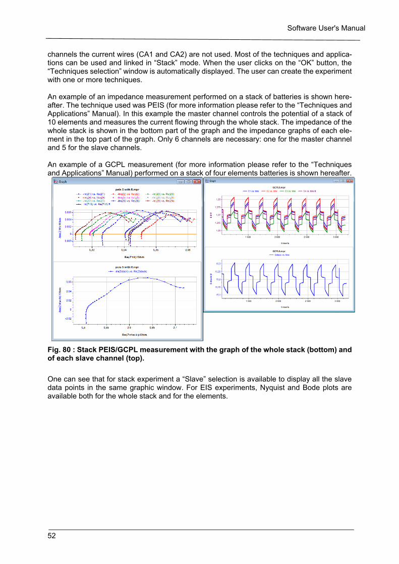
Software User's Manual
52
channels the current wires (CA1 and CA2) are not used. Most of the techniques and applica-tions can be used and linked in “Stack” mode. When the user clicks on the “OK” button, the “Techniques selection” window is automatically displayed. The user can create the experiment with one or more techniques. An example of an impedance measurement performed on a stack of batteries is shown here-after. The technique used was PEIS (for more information please refer to the “Techniques and Applications” Manual). In this example the master channel controls the potential of a stack of 10 elements and measures the current flowing through the whole stack. The impedance of the whole stack is shown in the bottom part of the graph and the impedance graphs of each ele-ment in the top part of the graph. Only 6 channels are necessary: one for the master channel and 5 for the slave channels. An example of a GCPL measurement (for more information please refer to the “Techniques and Applications” Manual) performed on a stack of four elements batteries is shown hereafter.
Fig. 80 : Stack PEIS/GCPL measurement with the graph of the whole stack (bottom) and of each slave channel (top).
One can see that for stack experiment a “Slave” selection is available to display all the slave data points in the same graphic window. For EIS experiments, Nyquist and Bode plots are available both for the whole stack and for the elements.
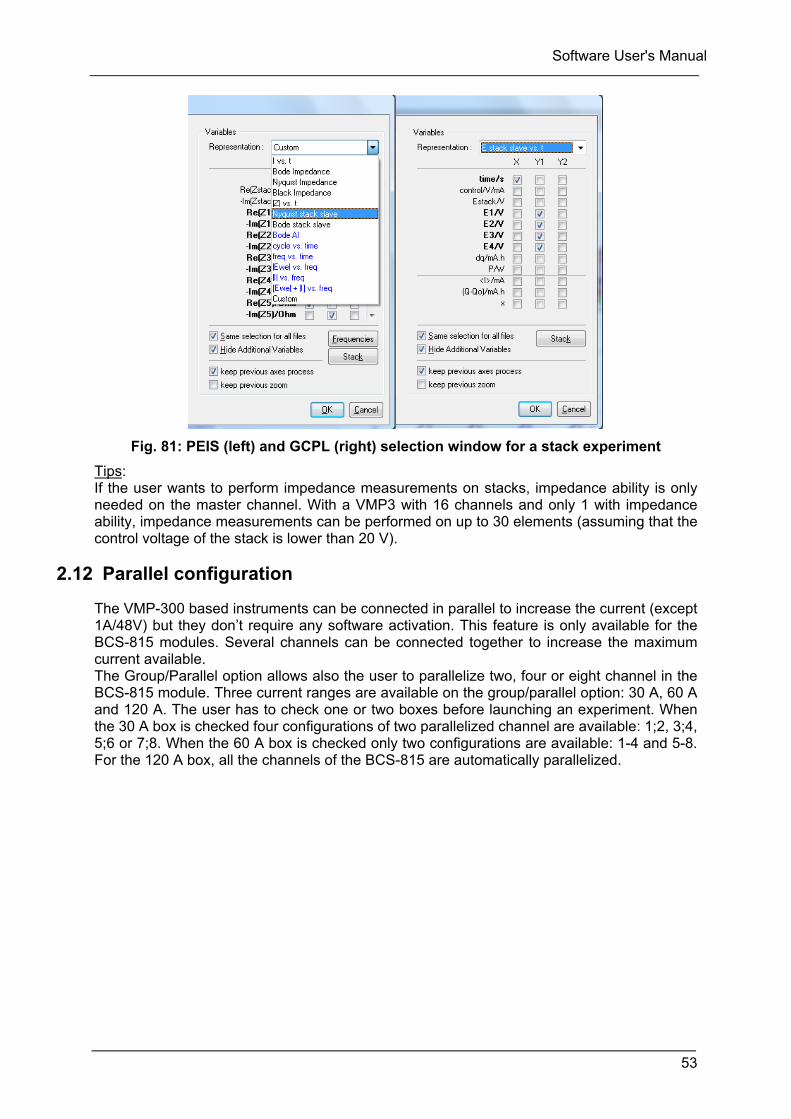
Software User's Manual
53
Fig. 81: PEIS (left) and GCPL (right) selection window for a stack experiment
Tips: If the user wants to perform impedance measurements on stacks, impedance ability is only needed on the master channel. With a VMP3 with 16 channels and only 1 with impedance ability, impedance measurements can be performed on up to 30 elements (assuming that the control voltage of the stack is lower than 20 V).
2.12 Parallel configuration
The VMP-300 based instruments can be connected in parallel to increase the current (except 1A/48V) but they don’t require any software activation. This feature is only available for the BCS-815 modules. Several channels can be connected together to increase the maximum current available. The Group/Parallel option allows also the user to parallelize two, four or eight channel in the BCS-815 module. Three current ranges are available on the group/parallel option: 30 A, 60 A and 120 A. The user has to check one or two boxes before launching an experiment. When the 30 A box is checked four configurations of two parallelized channel are available: 1;2, 3;4, 5;6 or 7;8. When the 60 A box is checked only two configurations are available: 1-4 and 5-8. For the 120 A box, all the channels of the BCS-815 are automatically parallelized.
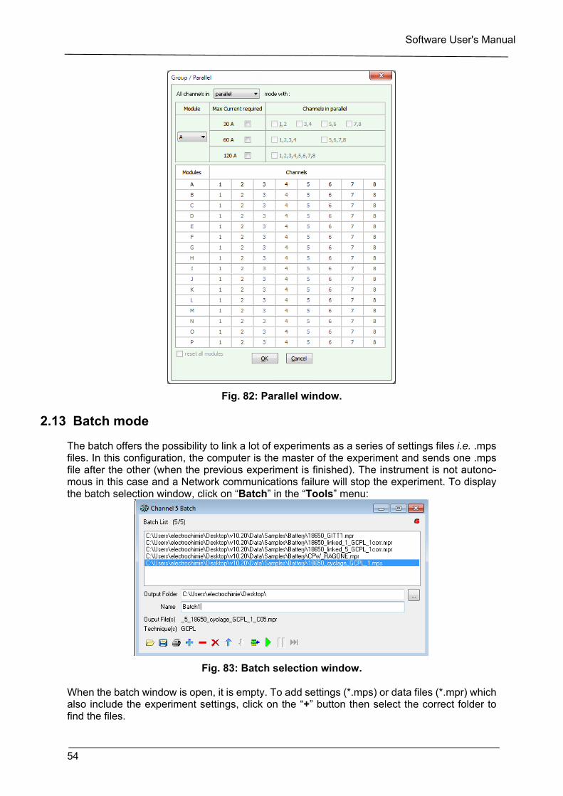
Software User's Manual
54
Fig. 82: Parallel window.
2.13 Batch mode
The batch offers the possibility to link a lot of experiments as a series of settings files i.e. .mps files. In this configuration, the computer is the master of the experiment and sends one .mps file after the other (when the previous experiment is finished). The instrument is not autono-mous in this case and a Network communications failure will stop the experiment. To display the batch selection window, click on “Batch” in the “Tools” menu:
Fig. 83: Batch selection window.
When the batch window is open, it is empty. To add settings (*.mps) or data files (*.mpr) which also include the experiment settings, click on the “+” button then select the correct folder to find the files.
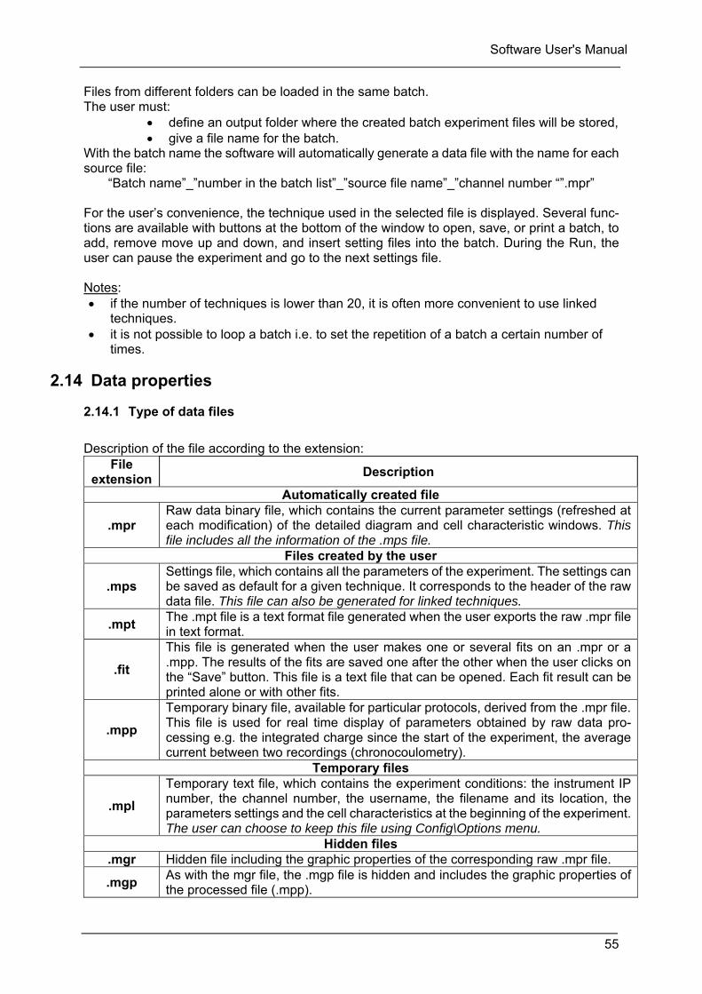
Software User's Manual
55
Files from different folders can be loaded in the same batch. The user must:
define an output folder where the created batch experiment files will be stored, give a file name for the batch.
With the batch name the software will automatically generate a data file with the name for each source file:
“Batch name”_”number in the batch list”_”source file name”_”channel number “”.mpr” For the user’s convenience, the technique used in the selected file is displayed. Several func-tions are available with buttons at the bottom of the window to open, save, or print a batch, to add, remove move up and down, and insert setting files into the batch. During the Run, the user can pause the experiment and go to the next settings file. Notes: if the number of techniques is lower than 20, it is often more convenient to use linked
techniques. it is not possible to loop a batch i.e. to set the repetition of a batch a certain number of
times.
2.14 Data properties
2.14.1 Type of data files
Description of the file according to the extension:
File extension
Description
Automatically created file
.mpr Raw data binary file, which contains the current parameter settings (refreshed at each modification) of the detailed diagram and cell characteristic windows. This file includes all the information of the .mps file.
Files created by the user
.mps Settings file, which contains all the parameters of the experiment. The settings can be saved as default for a given technique. It corresponds to the header of the raw data file. This file can also be generated for linked techniques.
.mpt The .mpt file is a text format file generated when the user exports the raw .mpr file in text format.
.fit
This file is generated when the user makes one or several fits on an .mpr or a .mpp. The results of the fits are saved one after the other when the user clicks on the “Save” button. This file is a text file that can be opened. Each fit result can be printed alone or with other fits.
.mpp
Temporary binary file, available for particular protocols, derived from the .mpr file. This file is used for real time display of parameters obtained by raw data pro-cessing e.g. the integrated charge since the start of the experiment, the average current between two recordings (chronocoulometry).
Temporary files
.mpl
Temporary text file, which contains the experiment conditions: the instrument IP number, the channel number, the username, the filename and its location, the parameters settings and the cell characteristics at the beginning of the experiment. The user can choose to keep this file using Config\Options menu.
Hidden files .mgr Hidden file including the graphic properties of the corresponding raw .mpr file.
.mgp As with the mgr file, the .mgp file is hidden and includes the graphic properties of the processed file (.mpp).
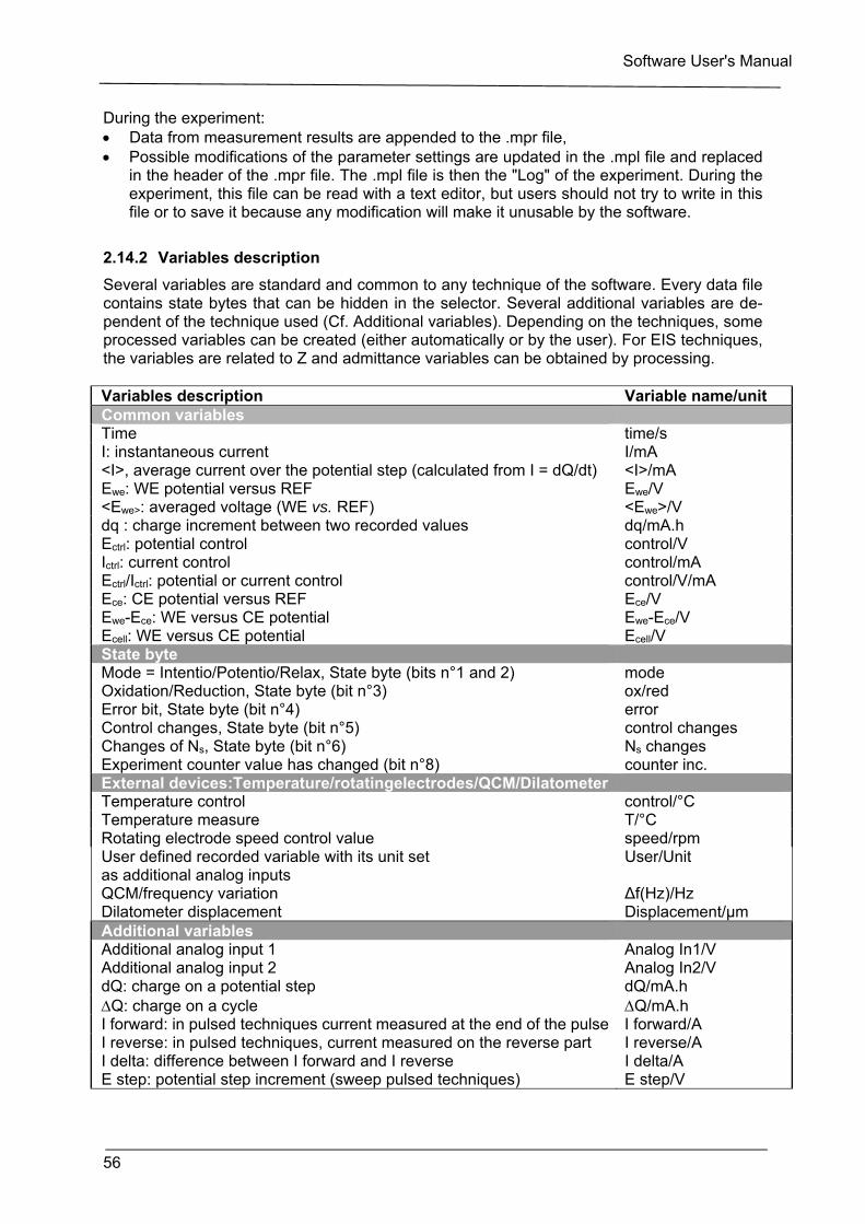
Software User's Manual
56
During the experiment: Data from measurement results are appended to the .mpr file, Possible modifications of the parameter settings are updated in the .mpl file and replaced
in the header of the .mpr file. The .mpl file is then the "Log" of the experiment. During the experiment, this file can be read with a text editor, but users should not try to write in this file or to save it because any modification will make it unusable by the software.
2.14.2 Variables description
Several variables are standard and common to any technique of the software. Every data file contains state bytes that can be hidden in the selector. Several additional variables are de-pendent of the technique used (Cf. Additional variables). Depending on the techniques, some processed variables can be created (either automatically or by the user). For EIS techniques, the variables are related to Z and admittance variables can be obtained by processing. Variables description Variable name/unit Common variables Time time/s I: instantaneous current I/mA <I>, average current over the potential step (calculated from I = dQ/dt) <I>/mA Ewe: WE potential versus REF Ewe/V <Ewe>: averaged voltage (WE vs. REF) <Ewe>/V dq : charge increment between two recorded values dq/mA.h Ectrl: potential control control/V Ictrl: current control control/mA Ectrl/Ictrl: potential or current control control/V/mA Ece: CE potential versus REF Ece/V Ewe-Ece: WE versus CE potential Ewe-Ece/V Ecell: WE versus CE potential Ecell/V State byte Mode = Intentio/Potentio/Relax, State byte (bits n°1 and 2) mode Oxidation/Reduction, State byte (bit n°3) ox/red Error bit, State byte (bit n°4) error Control changes, State byte (bit n°5) control changes Changes of Ns, State byte (bit n°6) Ns changes Experiment counter value has changed (bit n°8) counter inc. External devices:Temperature/rotatingelectrodes/QCM/Dilatometer Temperature control control/°C Temperature measure T/°C Rotating electrode speed control value speed/rpm User defined recorded variable with its unit set as additional analog inputs QCM/frequency variation Dilatometer displacement
User/Unit ∆f(Hz)/Hz Displacement/µm
Additional variables Additional analog input 1 Analog In1/V Additional analog input 2 Analog In2/V dQ: charge on a potential step dQ/mA.h Q: charge on a cycle Q/mA.h I forward: in pulsed techniques current measured at the end of the pulse I forward/A I reverse: in pulsed techniques, current measured on the reverse part I reverse/A I delta: difference between I forward and I reverse I delta/A E step: potential step increment (sweep pulsed techniques) E step/V
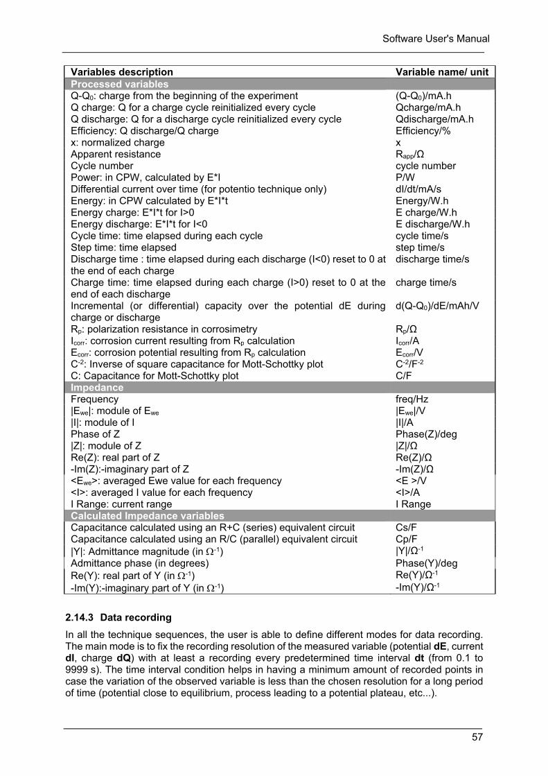
Software User's Manual
57
Variables description Variable name/ unit Processed variables Q-Q0: charge from the beginning of the experiment (Q-Q0)/mA.h Q charge: Q for a charge cycle reinitialized every cycle Qcharge/mA.h Q discharge: Q for a discharge cycle reinitialized every cycle Qdischarge/mA.h Efficiency: Q discharge/Q charge Efficiency/% x: normalized charge x Apparent resistance Rapp/Ω Cycle number cycle number Power: in CPW, calculated by E*I P/W Differential current over time (for potentio technique only) dI/dt/mA/s Energy: in CPW calculated by E*I*t Energy/W.h Energy charge: E*I*t for I>0 E charge/W.h Energy discharge: E*I*t for I<0 E discharge/W.h Cycle time: time elapsed during each cycle cycle time/s Step time: time elapsed step time/s Discharge time : time elapsed during each discharge (I<0) reset to 0 at the end of each charge
discharge time/s
Charge time: time elapsed during each charge (I>0) reset to 0 at the end of each discharge
charge time/s
Incremental (or differential) capacity over the potential dE during charge or discharge
d(Q-Q0)/dE/mAh/V
Rp: polarization resistance in corrosimetry Rp/Ω Icorr: corrosion current resulting from Rp calculation Icorr/A Ecorr: corrosion potential resulting from Rp calculation Ecorr/V C-2: Inverse of square capacitance for Mott-Schottky plot C-2/F-2 C: Capacitance for Mott-Schottky plot C/F Impedance Frequency freq/Hz |Ewe|: module of Ewe |Ewe|/V |I|: module of I |I|/A Phase of Z Phase(Z)/deg |Z|: module of Z |Z|/Ω Re(Z): real part of Z Re(Z)/Ω -Im(Z):-imaginary part of Z -Im(Z)/Ω <Ewe>: averaged Ewe value for each frequency <E >/V <I>: averaged I value for each frequency <I>/A I Range: current range I Range Calculated Impedance variables Capacitance calculated using an R+C (series) equivalent circuit Cs/F Capacitance calculated using an R/C (parallel) equivalent circuit Cp/F |Y|: Admittance magnitude (in -1) |Y|/Ω-1 Admittance phase (in degrees) Phase(Y)/deg Re(Y): real part of Y (in -1) Re(Y)/Ω-1 -Im(Y):-imaginary part of Y (in -1) -Im(Y)/Ω-1
2.14.3 Data recording
In all the technique sequences, the user is able to define different modes for data recording. The main mode is to fix the recording resolution of the measured variable (potential dE, current dI, charge dQ) with at least a recording every predetermined time interval dt (from 0.1 to 9999 s). The time interval condition helps in having a minimum amount of recorded points in case the variation of the observed variable is less than the chosen resolution for a long period of time (potential close to equilibrium, process leading to a potential plateau, etc...).
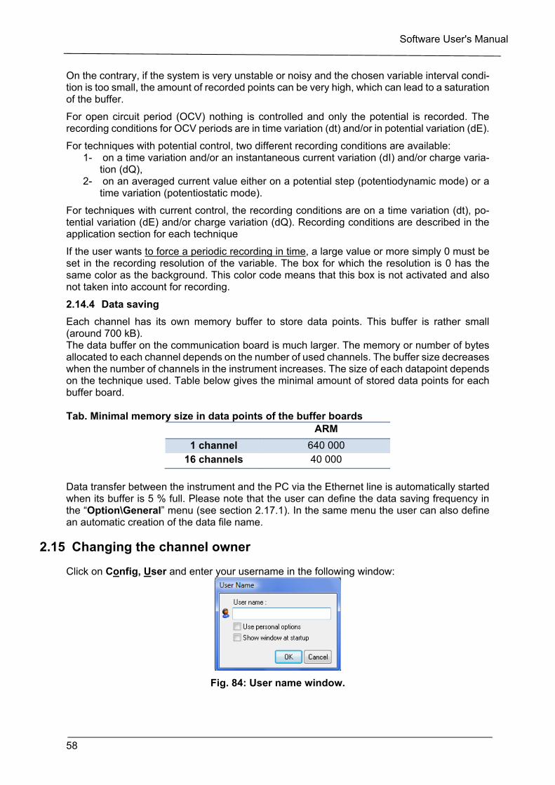
Software User's Manual
58
On the contrary, if the system is very unstable or noisy and the chosen variable interval condi-tion is too small, the amount of recorded points can be very high, which can lead to a saturation of the buffer.
For open circuit period (OCV) nothing is controlled and only the potential is recorded. The recording conditions for OCV periods are in time variation (dt) and/or in potential variation (dE).
For techniques with potential control, two different recording conditions are available: 1- on a time variation and/or an instantaneous current variation (dI) and/or charge varia-
tion (dQ), 2- on an averaged current value either on a potential step (potentiodynamic mode) or a
time variation (potentiostatic mode).
For techniques with current control, the recording conditions are on a time variation (dt), po-tential variation (dE) and/or charge variation (dQ). Recording conditions are described in the application section for each technique
If the user wants to force a periodic recording in time, a large value or more simply 0 must be set in the recording resolution of the variable. The box for which the resolution is 0 has the same color as the background. This color code means that this box is not activated and also not taken into account for recording.
2.14.4 Data saving
Each channel has its own memory buffer to store data points. This buffer is rather small (around 700 kB). The data buffer on the communication board is much larger. The memory or number of bytes allocated to each channel depends on the number of used channels. The buffer size decreases when the number of channels in the instrument increases. The size of each datapoint depends on the technique used. Table below gives the minimal amount of stored data points for each buffer board. Tab. Minimal memory size in data points of the buffer boards
ARM
1 channel 640 000 16 channels 40 000
Data transfer between the instrument and the PC via the Ethernet line is automatically started when its buffer is 5 % full. Please note that the user can define the data saving frequency in the “Option\General” menu (see section 2.17.1). In the same menu the user can also define an automatic creation of the data file name.
2.15 Changing the channel owner
Click on Config, User and enter your username in the following window:
Fig. 84: User name window.
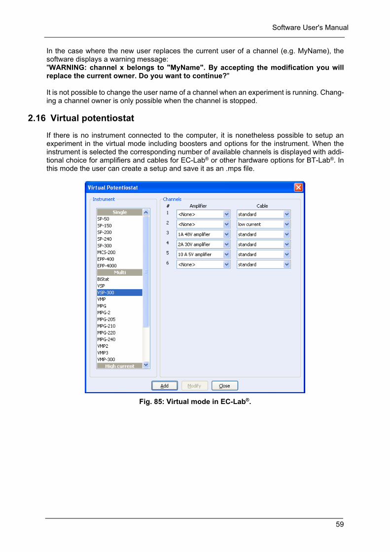
Software User's Manual
59
In the case where the new user replaces the current user of a channel (e.g. MyName), the software displays a warning message: "WARNING: channel x belongs to "MyName". By accepting the modification you will replace the current owner. Do you want to continue?" It is not possible to change the user name of a channel when an experiment is running. Chang-ing a channel owner is only possible when the channel is stopped.
2.16 Virtual potentiostat
If there is no instrument connected to the computer, it is nonetheless possible to setup an experiment in the virtual mode including boosters and options for the instrument. When the instrument is selected the corresponding number of available channels is displayed with addi-tional choice for amplifiers and cables for EC-Lab® or other hardware options for BT-Lab®. In this mode the user can create a setup and save it as an .mps file.
Fig. 85: Virtual mode in EC-Lab®.
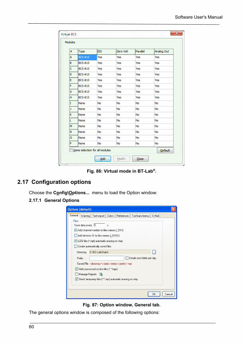
Software User's Manual
60
Fig. 86: Virtual mode in BT-Lab®.
2.17 Configuration options
Choose the Config\Options... menu to load the Option window:
2.17.1 General Options
Fig. 87: Option window, General tab.
The general options window is composed of the following options:
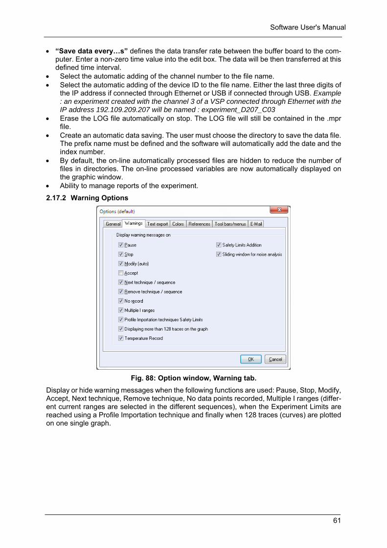
Software User's Manual
61
“Save data every…s” defines the data transfer rate between the buffer board to the com-puter. Enter a non-zero time value into the edit box. The data will be then transferred at this defined time interval.
Select the automatic adding of the channel number to the file name. Select the automatic adding of the device ID to the file name. Either the last three digits of
the IP address if connected through Ethernet or USB if connected through USB. Example : an experiment created with the channel 3 of a VSP connected through Ethernet with the IP address 192.109.209.207 will be named : experiment_D207_C03
Erase the LOG file automatically on stop. The LOG file will still be contained in the .mpr file.
Create an automatic data saving. The user must choose the directory to save the data file. The prefix name must be defined and the software will automatically add the date and the index number.
By default, the on-line automatically processed files are hidden to reduce the number of files in directories. The on-line processed variables are now automatically displayed on the graphic window.
Ability to manage reports of the experiment.
2.17.2 Warning Options
Fig. 88: Option window, Warning tab.
Display or hide warning messages when the following functions are used: Pause, Stop, Modify, Accept, Next technique, Remove technique, No data points recorded, Multiple I ranges (differ-ent current ranges are selected in the different sequences), when the Experiment Limits are reached using a Profile Importation technique and finally when 128 traces (curves) are plotted on one single graph.
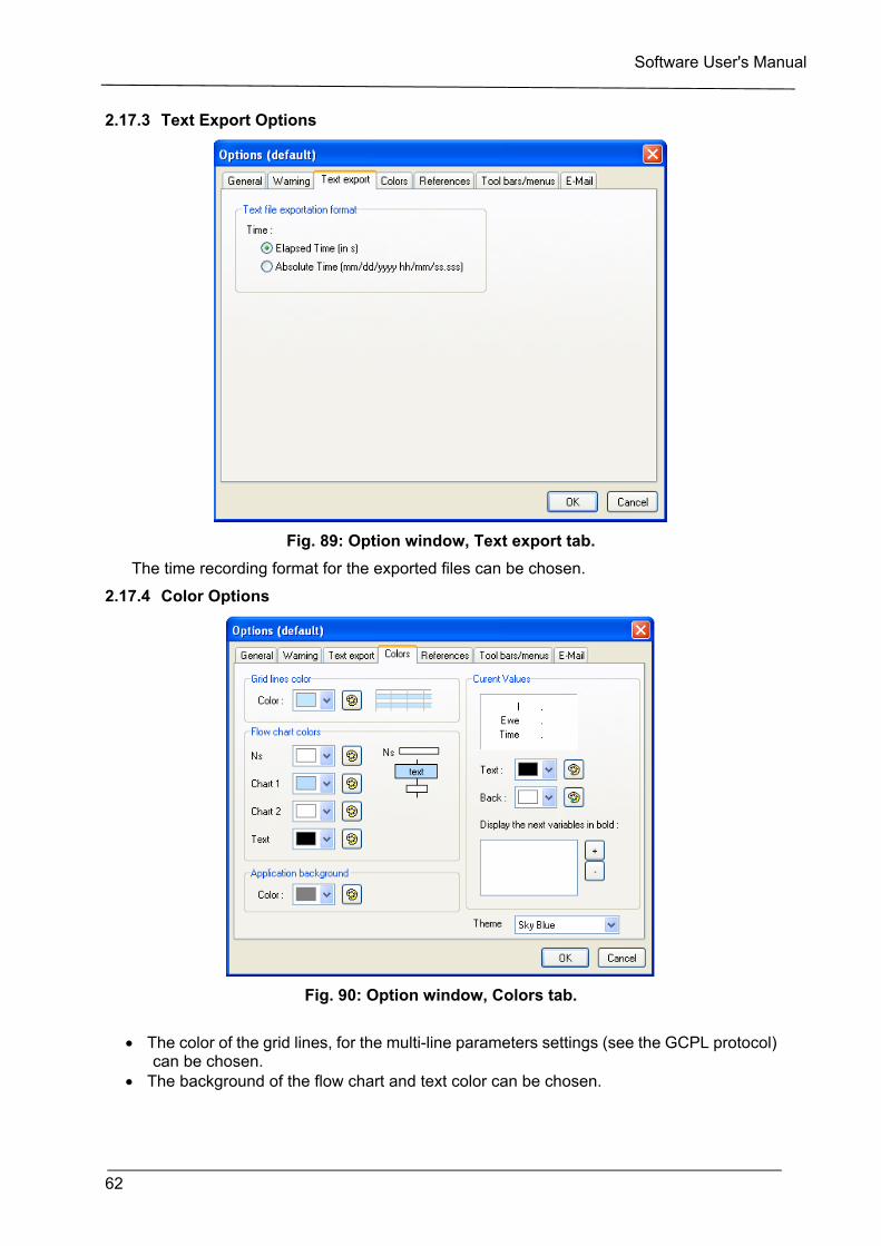
Software User's Manual
62
2.17.3 Text Export Options
Fig. 89: Option window, Text export tab.
The time recording format for the exported files can be chosen.
2.17.4 Color Options
Fig. 90: Option window, Colors tab.
The color of the grid lines, for the multi-line parameters settings (see the GCPL protocol)
can be chosen. The background of the flow chart and text color can be chosen.
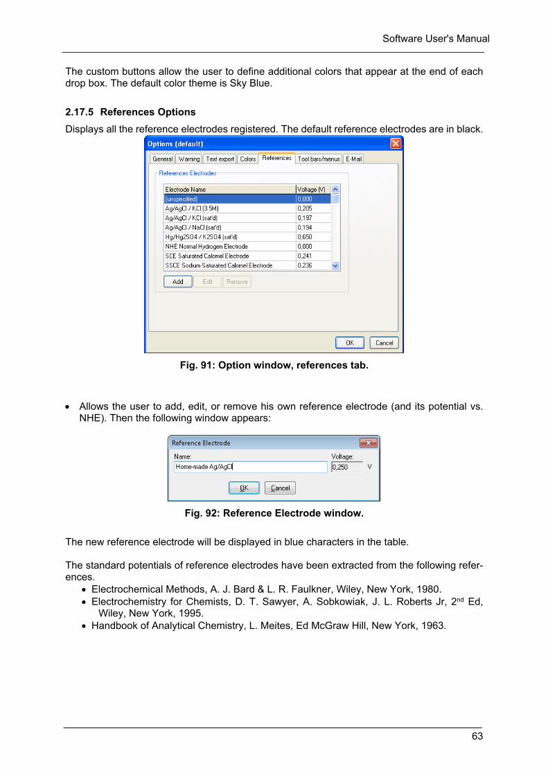
Software User's Manual
63
The custom buttons allow the user to define additional colors that appear at the end of each drop box. The default color theme is Sky Blue.
2.17.5 References Options
Displays all the reference electrodes registered. The default reference electrodes are in black.
Fig. 91: Option window, references tab.
Allows the user to add, edit, or remove his own reference electrode (and its potential vs.
NHE). Then the following window appears:
Fig. 92: Reference Electrode window.
The new reference electrode will be displayed in blue characters in the table. The standard potentials of reference electrodes have been extracted from the following refer-ences.
Electrochemical Methods, A. J. Bard & L. R. Faulkner, Wiley, New York, 1980. Electrochemistry for Chemists, D. T. Sawyer, A. Sobkowiak, J. L. Roberts Jr, 2nd Ed,
Wiley, New York, 1995. Handbook of Analytical Chemistry, L. Meites, Ed McGraw Hill, New York, 1963.
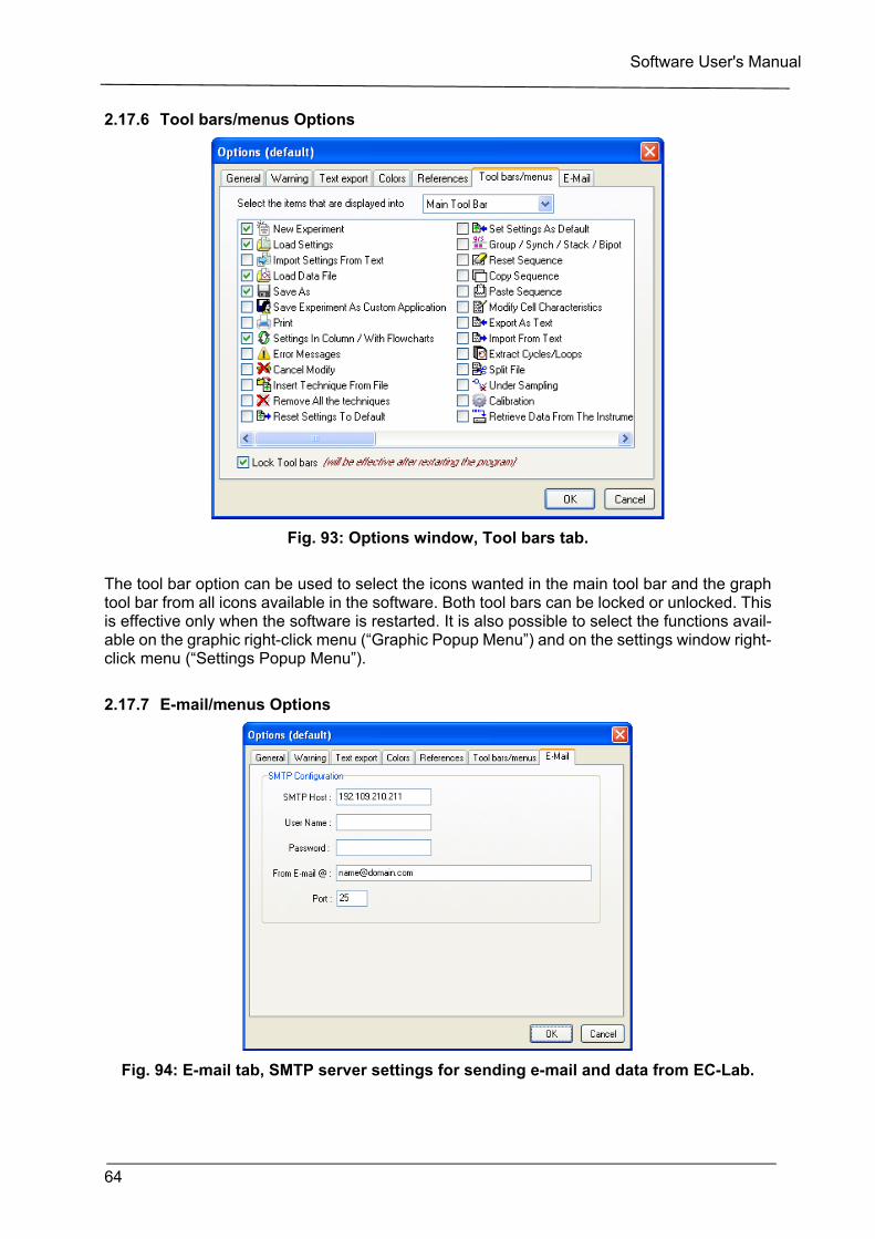
Software User's Manual
64
2.17.6 Tool bars/menus Options
Fig. 93: Options window, Tool bars tab.
The tool bar option can be used to select the icons wanted in the main tool bar and the graph tool bar from all icons available in the software. Both tool bars can be locked or unlocked. This is effective only when the software is restarted. It is also possible to select the functions avail-able on the graphic right-click menu (“Graphic Popup Menu”) and on the settings window right-click menu (“Settings Popup Menu”).
2.17.7 E-mail/menus Options
Fig. 94: E-mail tab, SMTP server settings for sending e-mail and data from EC-Lab.
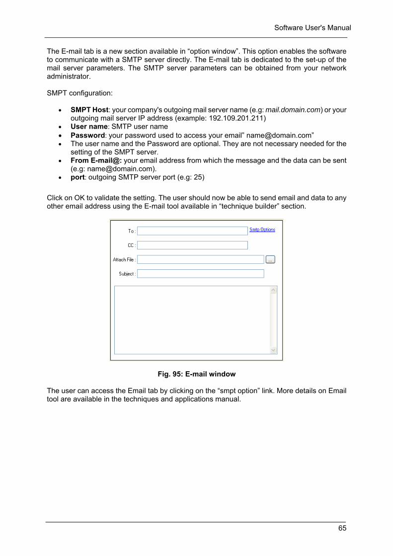
Software User's Manual
65
The E-mail tab is a new section available in “option window”. This option enables the software to communicate with a SMTP server directly. The E-mail tab is dedicated to the set-up of the mail server parameters. The SMTP server parameters can be obtained from your network administrator. SMPT configuration:
SMPT Host: your company's outgoing mail server name (e.g: mail.domain.com) or your outgoing mail server IP address (example: 192.109.201.211)
User name: SMTP user name Password: your password used to access your email” [email protected]” The user name and the Password are optional. They are not necessary needed for the
setting of the SMPT server. From E-mail@: your email address from which the message and the data can be sent
(e.g: [email protected]). port: outgoing SMTP server port (e.g: 25)
Click on OK to validate the setting. The user should now be able to send email and data to any other email address using the E-mail tool available in “technique builder” section.
Fig. 95: E-mail window The user can access the Email tab by clicking on the “smpt option” link. More details on Email tool are available in the techniques and applications manual.
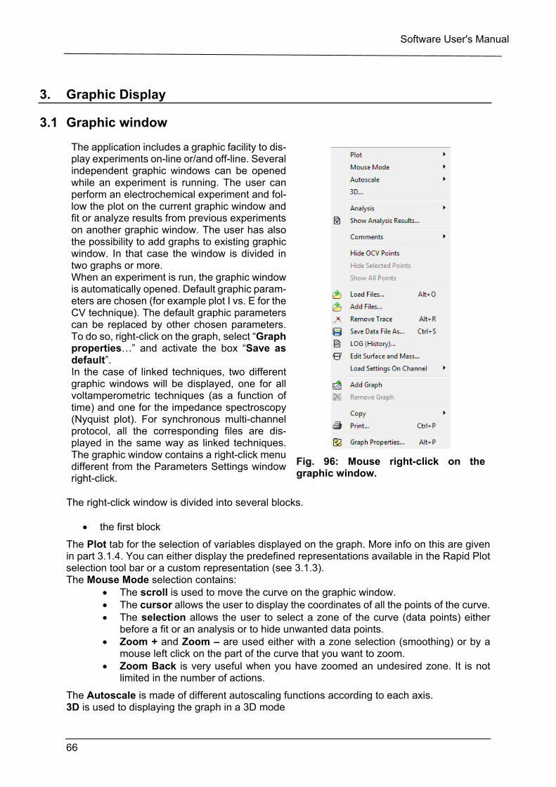
Software User's Manual
66
3. Graphic Display
3.1 Graphic window
The application includes a graphic facility to dis-play experiments on-line or/and off-line. Several independent graphic windows can be opened while an experiment is running. The user can perform an electrochemical experiment and fol-low the plot on the current graphic window and fit or analyze results from previous experiments on another graphic window. The user has also the possibility to add graphs to existing graphic window. In that case the window is divided in two graphs or more. When an experiment is run, the graphic window is automatically opened. Default graphic param-eters are chosen (for example plot I vs. E for the CV technique). The default graphic parameters can be replaced by other chosen parameters. To do so, right-click on the graph, select “Graph properties…” and activate the box “Save as default”. In the case of linked techniques, two different graphic windows will be displayed, one for all voltamperometric techniques (as a function of time) and one for the impedance spectroscopy (Nyquist plot). For synchronous multi-channel protocol, all the corresponding files are dis-played in the same way as linked techniques. The graphic window contains a right-click menu different from the Parameters Settings window right-click.
Fig. 96: Mouse right-click on the graphic window.
The right-click window is divided into several blocks.
the first block
The Plot tab for the selection of variables displayed on the graph. More info on this are given in part 3.1.4. You can either display the predefined representations available in the Rapid Plot selection tool bar or a custom representation (see 3.1.3). The Mouse Mode selection contains:
The scroll is used to move the curve on the graphic window. The cursor allows the user to display the coordinates of all the points of the curve. The selection allows the user to select a zone of the curve (data points) either
before a fit or an analysis or to hide unwanted data points. Zoom + and Zoom – are used either with a zone selection (smoothing) or by a
mouse left click on the part of the curve that you want to zoom. Zoom Back is very useful when you have zoomed an undesired zone. It is not
limited in the number of actions.
The Autoscale is made of different autoscaling functions according to each axis. 3D is used to displaying the graph in a 3D mode
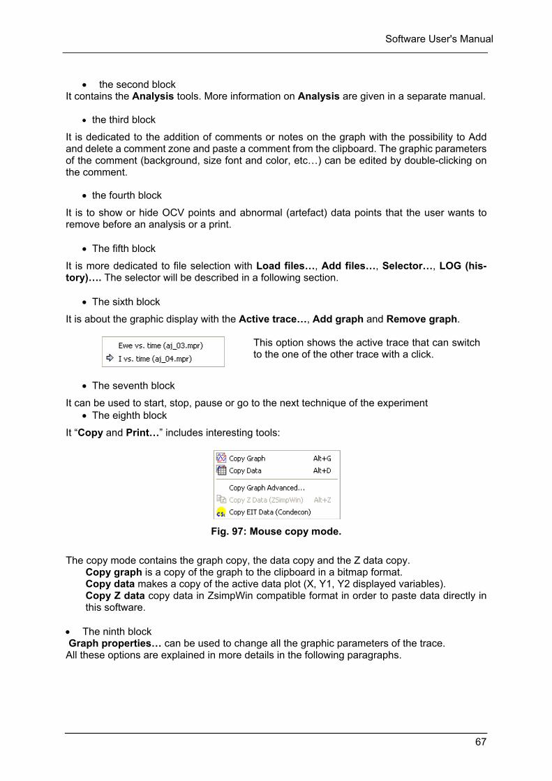
Software User's Manual
67
the second block
It contains the Analysis tools. More information on Analysis are given in a separate manual.
the third block
It is dedicated to the addition of comments or notes on the graph with the possibility to Add and delete a comment zone and paste a comment from the clipboard. The graphic parameters of the comment (background, size font and color, etc…) can be edited by double-clicking on the comment.
the fourth block
It is to show or hide OCV points and abnormal (artefact) data points that the user wants to remove before an analysis or a print.
The fifth block
It is more dedicated to file selection with Load files…, Add files…, Selector…, LOG (his-tory)…. The selector will be described in a following section.
The sixth block
It is about the graphic display with the Active trace…, Add graph and Remove graph.
This option shows the active trace that can switch to the one of the other trace with a click.
The seventh block
It can be used to start, stop, pause or go to the next technique of the experiment The eighth block
It “Copy and Print…” includes interesting tools:
Fig. 97: Mouse copy mode.
The copy mode contains the graph copy, the data copy and the Z data copy.
Copy graph is a copy of the graph to the clipboard in a bitmap format. Copy data makes a copy of the active data plot (X, Y1, Y2 displayed variables). Copy Z data copy data in ZsimpWin compatible format in order to paste data directly in this software.
The ninth block Graph properties… can be used to change all the graphic parameters of the trace. All these options are explained in more details in the following paragraphs.
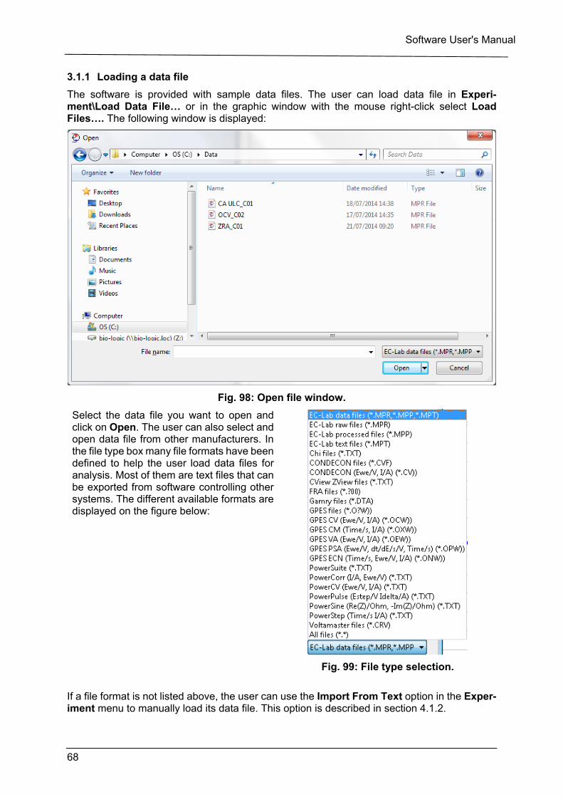
Software User's Manual
68
3.1.1 Loading a data file
The software is provided with sample data files. The user can load data file in Experi-ment\Load Data File… or in the graphic window with the mouse right-click select Load Files…. The following window is displayed:
Fig. 98: Open file window.
Select the data file you want to open and click on Open. The user can also select and open data file from other manufacturers. In the file type box many file formats have been defined to help the user load data files for analysis. Most of them are text files that can be exported from software controlling other systems. The different available formats are displayed on the figure below:
Fig. 99: File type selection.
If a file format is not listed above, the user can use the Import From Text option in the Exper-iment menu to manually load its data file. This option is described in section 4.1.2.
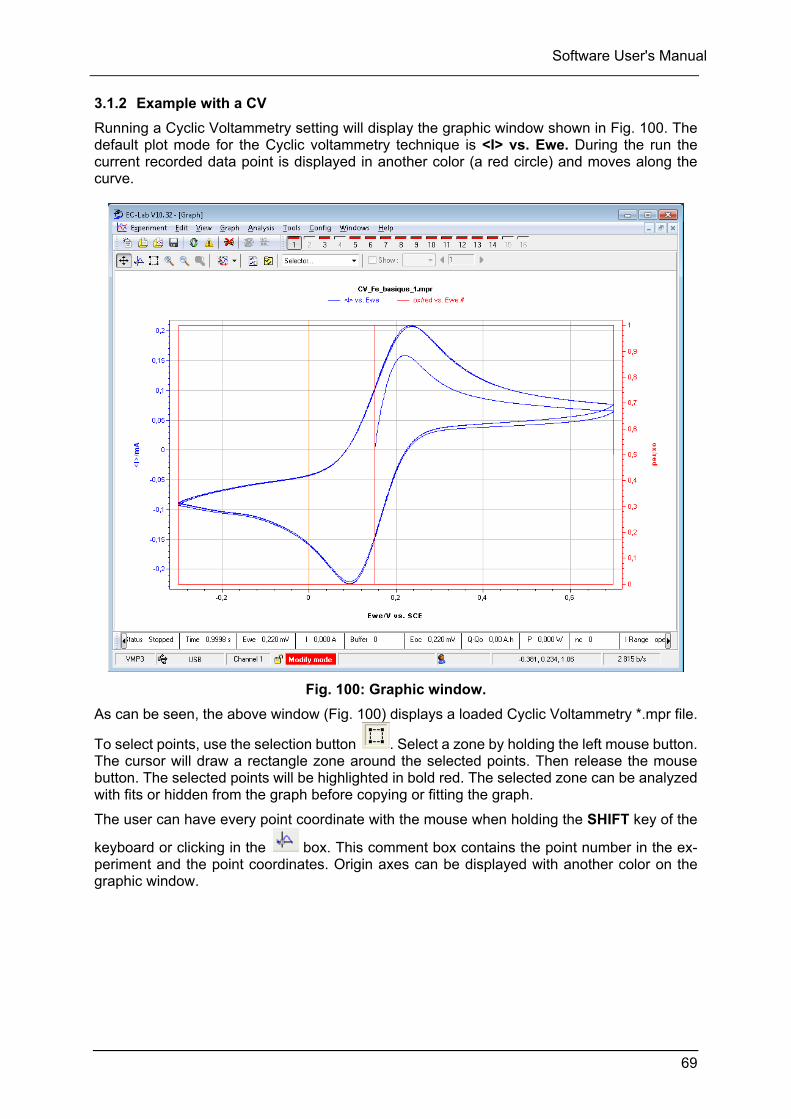
Software User's Manual
69
3.1.2 Example with a CV
Running a Cyclic Voltammetry setting will display the graphic window shown in Fig. 100. The default plot mode for the Cyclic voltammetry technique is <I> vs. Ewe. During the run the current recorded data point is displayed in another color (a red circle) and moves along the curve.
Fig. 100: Graphic window.
As can be seen, the above window (Fig. 100) displays a loaded Cyclic Voltammetry *.mpr file.
To select points, use the selection button . Select a zone by holding the left mouse button. The cursor will draw a rectangle zone around the selected points. Then release the mouse button. The selected points will be highlighted in bold red. The selected zone can be analyzed with fits or hidden from the graph before copying or fitting the graph.
The user can have every point coordinate with the mouse when holding the SHIFT key of the
keyboard or clicking in the box. This comment box contains the point number in the ex-periment and the point coordinates. Origin axes can be displayed with another color on the graphic window.
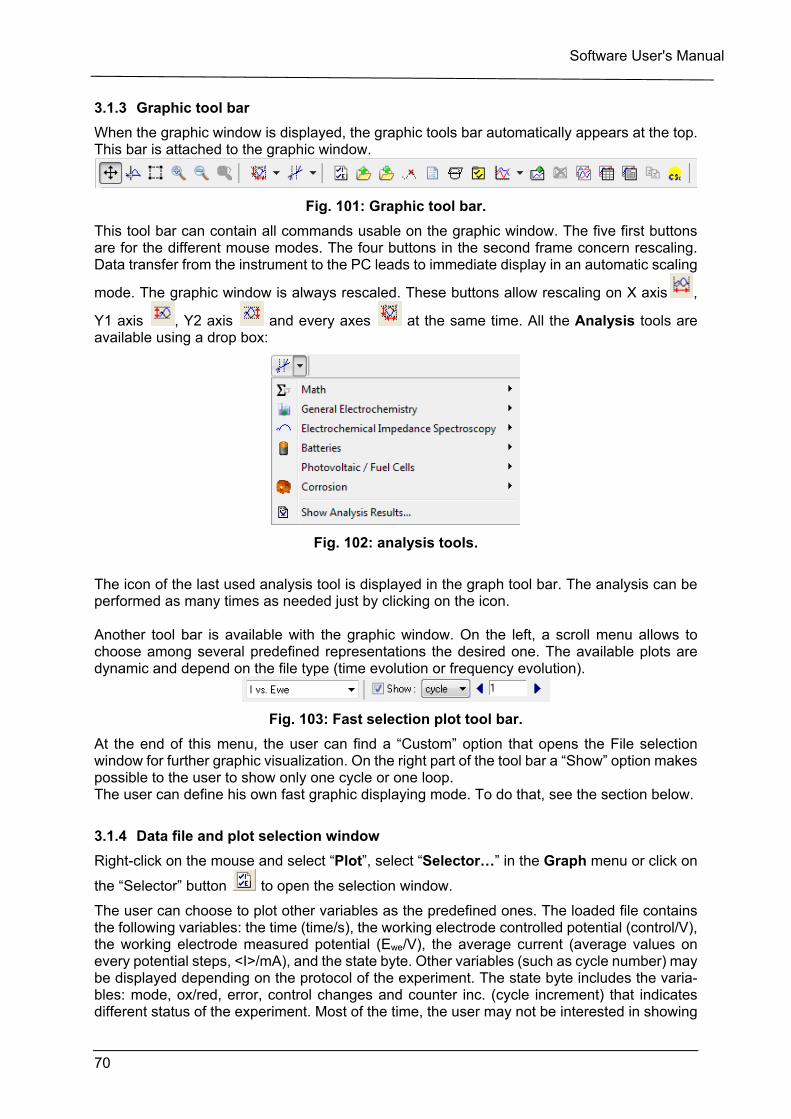
Software User's Manual
70
3.1.3 Graphic tool bar
When the graphic window is displayed, the graphic tools bar automatically appears at the top. This bar is attached to the graphic window.
Fig. 101: Graphic tool bar.
This tool bar can contain all commands usable on the graphic window. The five first buttons are for the different mouse modes. The four buttons in the second frame concern rescaling. Data transfer from the instrument to the PC leads to immediate display in an automatic scaling
mode. The graphic window is always rescaled. These buttons allow rescaling on X axis ,
Y1 axis , Y2 axis and every axes at the same time. All the Analysis tools are available using a drop box:
Fig. 102: analysis tools.
The icon of the last used analysis tool is displayed in the graph tool bar. The analysis can be performed as many times as needed just by clicking on the icon. Another tool bar is available with the graphic window. On the left, a scroll menu allows to choose among several predefined representations the desired one. The available plots are dynamic and depend on the file type (time evolution or frequency evolution).
Fig. 103: Fast selection plot tool bar.
At the end of this menu, the user can find a “Custom” option that opens the File selection window for further graphic visualization. On the right part of the tool bar a “Show” option makes possible to the user to show only one cycle or one loop. The user can define his own fast graphic displaying mode. To do that, see the section below.
3.1.4 Data file and plot selection window
Right-click on the mouse and select “Plot”, select “Selector…” in the Graph menu or click on
the “Selector” button to open the selection window.
The user can choose to plot other variables as the predefined ones. The loaded file contains the following variables: the time (time/s), the working electrode controlled potential (control/V), the working electrode measured potential (Ewe/V), the average current (average values on every potential steps, <I>/mA), and the state byte. Other variables (such as cycle number) may be displayed depending on the protocol of the experiment. The state byte includes the varia-bles: mode, ox/red, error, control changes and counter inc. (cycle increment) that indicates different status of the experiment. Most of the time, the user may not be interested in showing
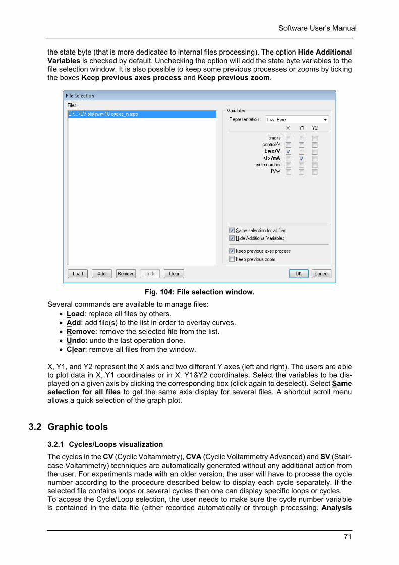
Software User's Manual
71
the state byte (that is more dedicated to internal files processing). The option Hide Additional Variables is checked by default. Unchecking the option will add the state byte variables to the file selection window. It is also possible to keep some previous processes or zooms by ticking the boxes Keep previous axes process and Keep previous zoom.
Fig. 104: File selection window.
Several commands are available to manage files: Load: replace all files by others. Add: add file(s) to the list in order to overlay curves. Remove: remove the selected file from the list. Undo: undo the last operation done. Clear: remove all files from the window.
X, Y1, and Y2 represent the X axis and two different Y axes (left and right). The users are able to plot data in X, Y1 coordinates or in X, Y1&Y2 coordinates. Select the variables to be dis-played on a given axis by clicking the corresponding box (click again to deselect). Select Same selection for all files to get the same axis display for several files. A shortcut scroll menu allows a quick selection of the graph plot.
3.2 Graphic tools
3.2.1 Cycles/Loops visualization
The cycles in the CV (Cyclic Voltammetry), CVA (Cyclic Voltammetry Advanced) and SV (Stair-case Voltammetry) techniques are automatically generated without any additional action from the user. For experiments made with an older version, the user will have to process the cycle number according to the procedure described below to display each cycle separately. If the selected file contains loops or several cycles then one can display specific loops or cycles. To access the Cycle/Loop selection, the user needs to make sure the cycle number variable is contained in the data file (either recorded automatically or through processing. Analysis
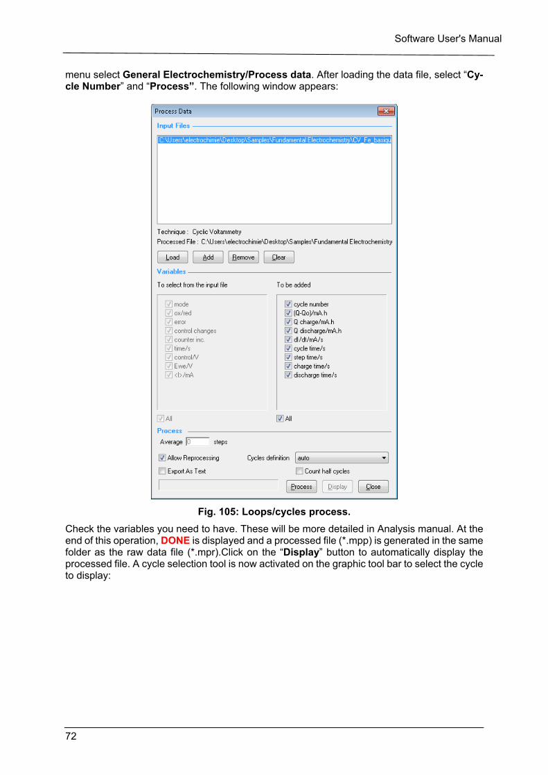
Software User's Manual
72
menu select General Electrochemistry/Process data. After loading the data file, select “Cy-cle Number” and “Process”. The following window appears:
Fig. 105: Loops/cycles process.
Check the variables you need to have. These will be more detailed in Analysis manual. At the end of this operation, DONE is displayed and a processed file (*.mpp) is generated in the same folder as the raw data file (*.mpr).Click on the “Display” button to automatically display the processed file. A cycle selection tool is now activated on the graphic tool bar to select the cycle to display:
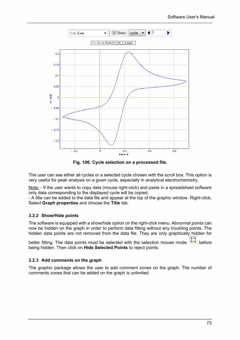
Software User's Manual
73
Fig. 106: Cycle selection on a processed file.
The user can see either all cycles or a selected cycle chosen with the scroll box. This option is very useful for peak analysis on a given cycle, especially in analytical electrochemistry.
Note: - If the user wants to copy data (mouse right-click) and paste in a spreadsheet software only data corresponding to the displayed cycle will be copied. - A title can be added to the data file and appear at the top of the graphic window. Right-click, Select Graph properties and choose the Title tab.
3.2.2 Show/Hide points
The software is equipped with a show/hide option on the right-click menu. Abnormal points can now be hidden on the graph in order to perform data fitting without any troubling points. The hidden data points are not removed from the data file. They are only graphically hidden for
better fitting. The data points must be selected with the selection mouse mode before being hidden. Then click on Hide Selected Points to reject points.
3.2.3 Add comments on the graph
The graphic package allows the user to add comment zones on the graph. The number of comments zones that can be added on the graph is unlimited.
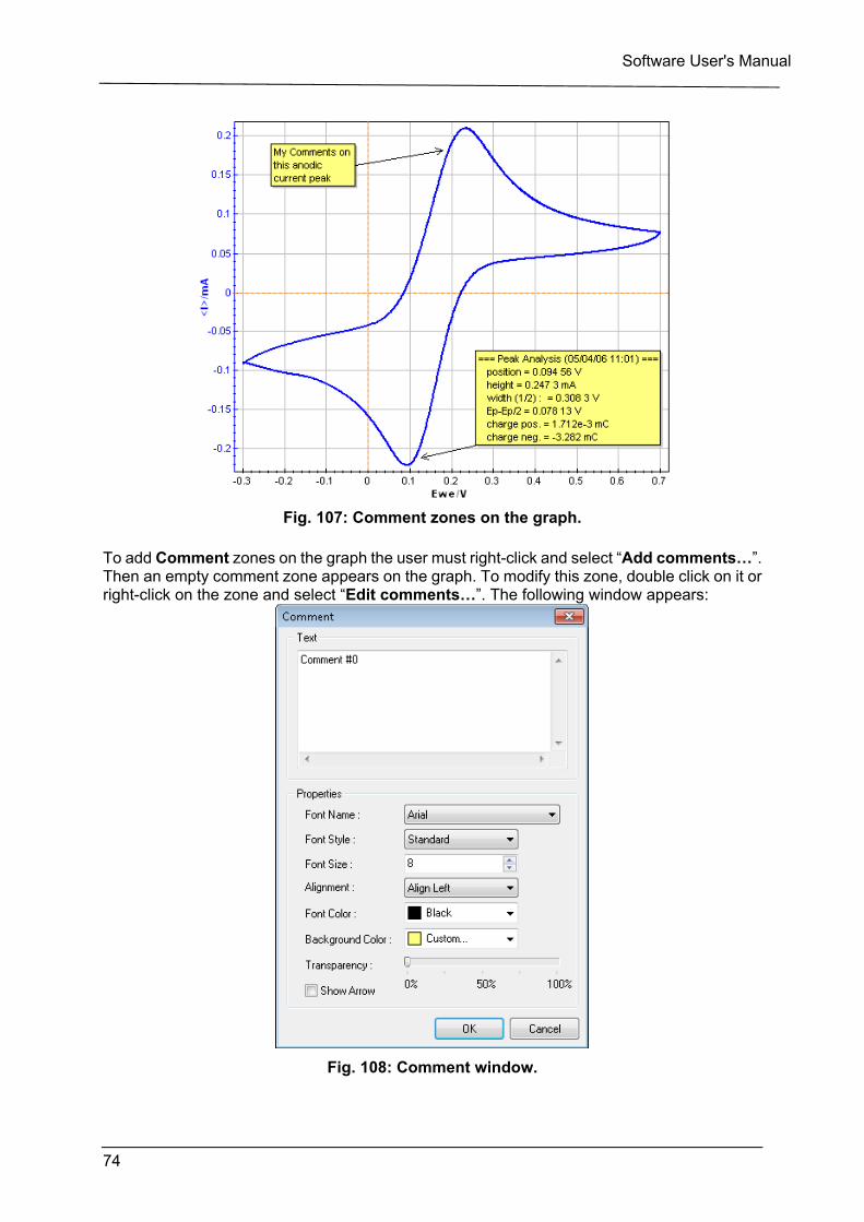
Software User's Manual
74
Fig. 107: Comment zones on the graph.
To add Comment zones on the graph the user must right-click and select “Add comments…”. Then an empty comment zone appears on the graph. To modify this zone, double click on it or right-click on the zone and select “Edit comments…”. The following window appears:
Fig. 108: Comment window.
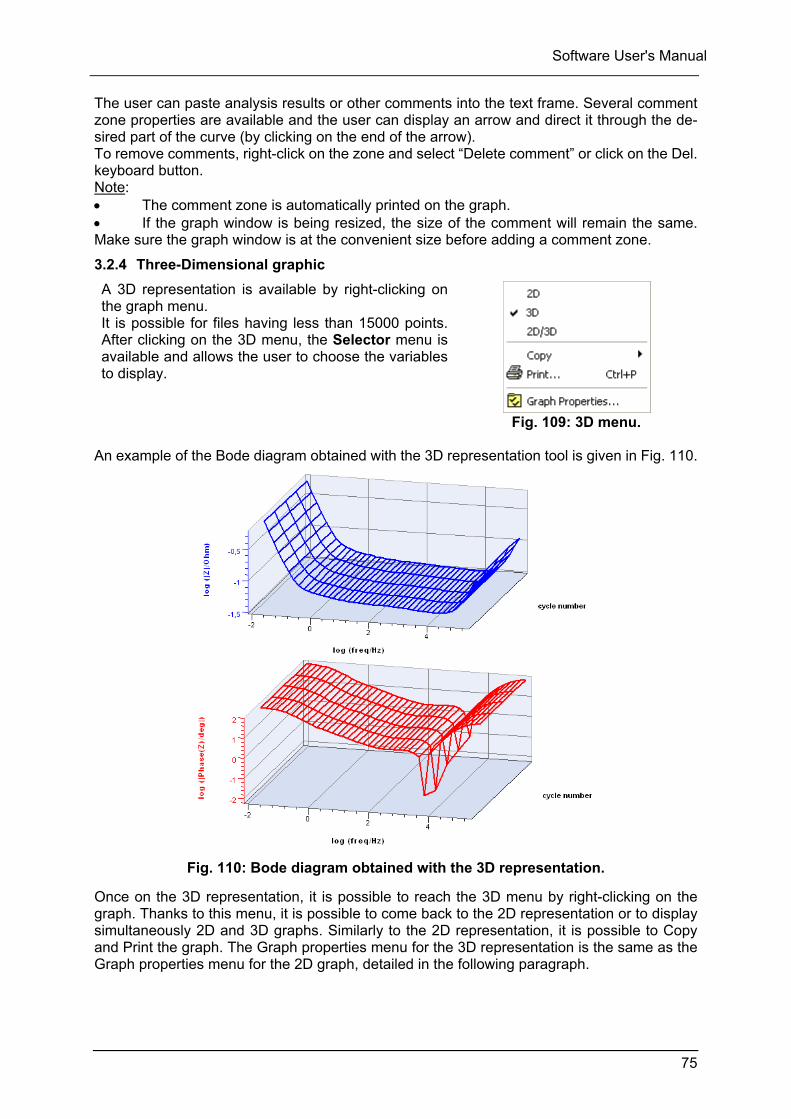
Software User's Manual
75
The user can paste analysis results or other comments into the text frame. Several comment zone properties are available and the user can display an arrow and direct it through the de-sired part of the curve (by clicking on the end of the arrow). To remove comments, right-click on the zone and select “Delete comment” or click on the Del. keyboard button. Note: The comment zone is automatically printed on the graph. If the graph window is being resized, the size of the comment will remain the same. Make sure the graph window is at the convenient size before adding a comment zone.
3.2.4 Three-Dimensional graphic
A 3D representation is available by right-clicking on the graph menu. It is possible for files having less than 15000 points. After clicking on the 3D menu, the Selector menu is available and allows the user to choose the variables to display.
Fig. 109: 3D menu.
An example of the Bode diagram obtained with the 3D representation tool is given in Fig. 110.
Fig. 110: Bode diagram obtained with the 3D representation.
Once on the 3D representation, it is possible to reach the 3D menu by right-clicking on the graph. Thanks to this menu, it is possible to come back to the 2D representation or to display simultaneously 2D and 3D graphs. Similarly to the 2D representation, it is possible to Copy and Print the graph. The Graph properties menu for the 3D representation is the same as the Graph properties menu for the 2D graph, detailed in the following paragraph.
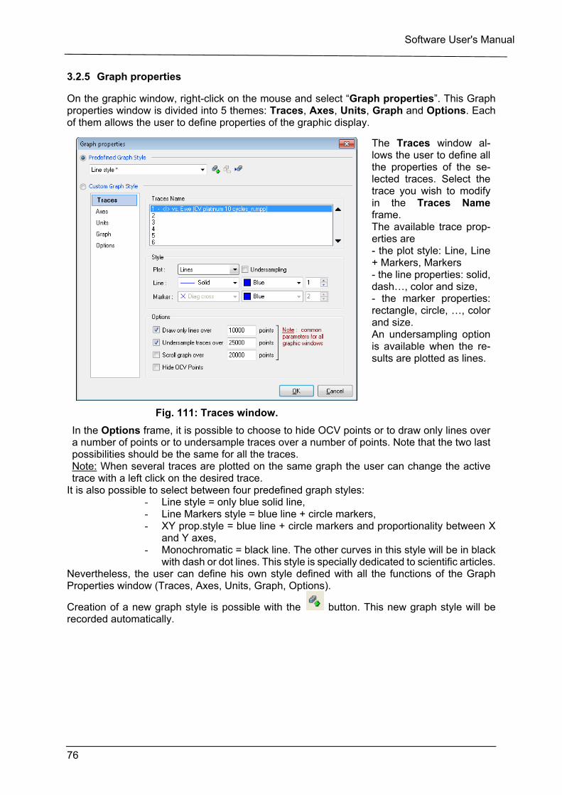
Software User's Manual
76
3.2.5 Graph properties
On the graphic window, right-click on the mouse and select “Graph properties”. This Graph properties window is divided into 5 themes: Traces, Axes, Units, Graph and Options. Each of them allows the user to define properties of the graphic display.
Fig. 111: Traces window.
The Traces window al-lows the user to define all the properties of the se-lected traces. Select the trace you wish to modify in the Traces Name frame. The available trace prop-erties are - the plot style: Line, Line + Markers, Markers - the line properties: solid, dash…, color and size, - the marker properties: rectangle, circle, …, color and size. An undersampling option is available when the re-sults are plotted as lines.
In the Options frame, it is possible to choose to hide OCV points or to draw only lines over a number of points or to undersample traces over a number of points. Note that the two last possibilities should be the same for all the traces. Note: When several traces are plotted on the same graph the user can change the active trace with a left click on the desired trace.
It is also possible to select between four predefined graph styles: - Line style = only blue solid line, - Line Markers style = blue line + circle markers, - XY prop.style = blue line + circle markers and proportionality between X
and Y axes, - Monochromatic = black line. The other curves in this style will be in black
with dash or dot lines. This style is specially dedicated to scientific articles. Nevertheless, the user can define his own style defined with all the functions of the Graph Properties window (Traces, Axes, Units, Graph, Options).
Creation of a new graph style is possible with the button. This new graph style will be recorded automatically.
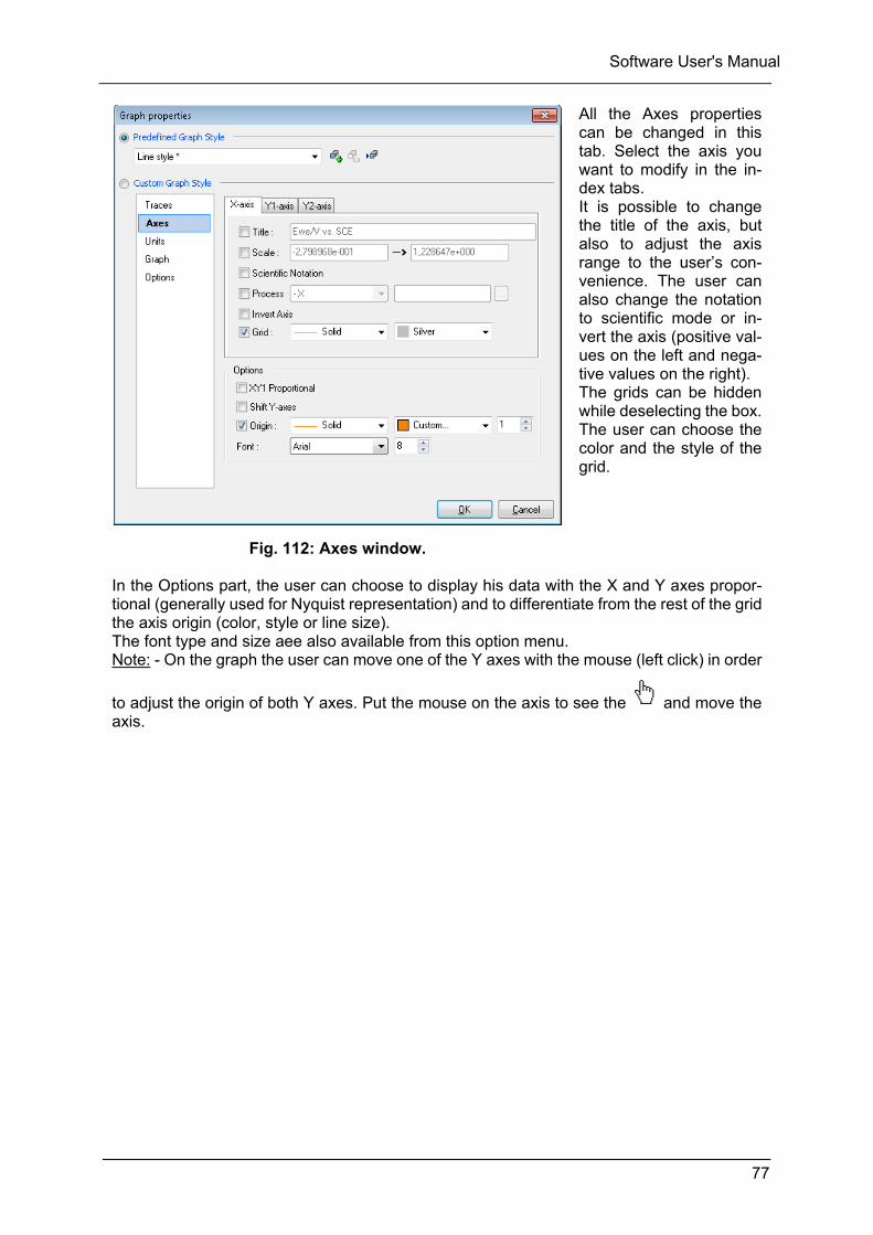
Software User's Manual
77
Fig. 112: Axes window.
All the Axes properties can be changed in this tab. Select the axis you want to modify in the in-dex tabs. It is possible to change the title of the axis, but also to adjust the axis range to the user’s con-venience. The user can also change the notation to scientific mode or in-vert the axis (positive val-ues on the left and nega-tive values on the right). The grids can be hidden while deselecting the box. The user can choose the color and the style of the grid.
In the Options part, the user can choose to display his data with the X and Y axes propor-tional (generally used for Nyquist representation) and to differentiate from the rest of the grid the axis origin (color, style or line size). The font type and size aee also available from this option menu. Note: - On the graph the user can move one of the Y axes with the mouse (left click) in order
to adjust the origin of both Y axes. Put the mouse on the axis to see the and move the axis.
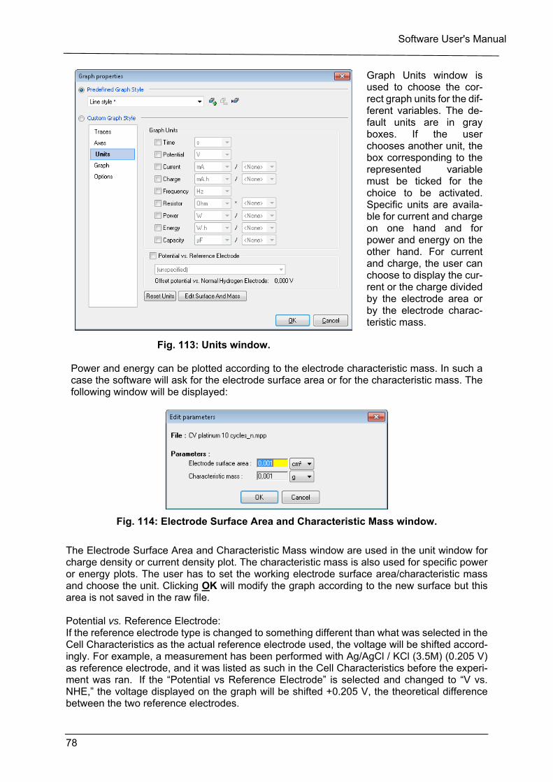
Software User's Manual
78
Fig. 113: Units window.
Graph Units window is used to choose the cor-rect graph units for the dif-ferent variables. The de-fault units are in gray boxes. If the user chooses another unit, the box corresponding to the represented variable must be ticked for the choice to be activated. Specific units are availa-ble for current and charge on one hand and for power and energy on the other hand. For current and charge, the user can choose to display the cur-rent or the charge divided by the electrode area or by the electrode charac-teristic mass.
Power and energy can be plotted according to the electrode characteristic mass. In such a case the software will ask for the electrode surface area or for the characteristic mass. The following window will be displayed:
Fig. 114: Electrode Surface Area and Characteristic Mass window.
The Electrode Surface Area and Characteristic Mass window are used in the unit window for charge density or current density plot. The characteristic mass is also used for specific power or energy plots. The user has to set the working electrode surface area/characteristic mass and choose the unit. Clicking OK will modify the graph according to the new surface but this area is not saved in the raw file. Potential vs. Reference Electrode: If the reference electrode type is changed to something different than what was selected in the Cell Characteristics as the actual reference electrode used, the voltage will be shifted accord-ingly. For example, a measurement has been performed with Ag/AgCl / KCl (3.5M) (0.205 V) as reference electrode, and it was listed as such in the Cell Characteristics before the experi-ment was ran. If the “Potential vs Reference Electrode” is selected and changed to “V vs. NHE,” the voltage displayed on the graph will be shifted +0.205 V, the theoretical difference between the two reference electrodes.
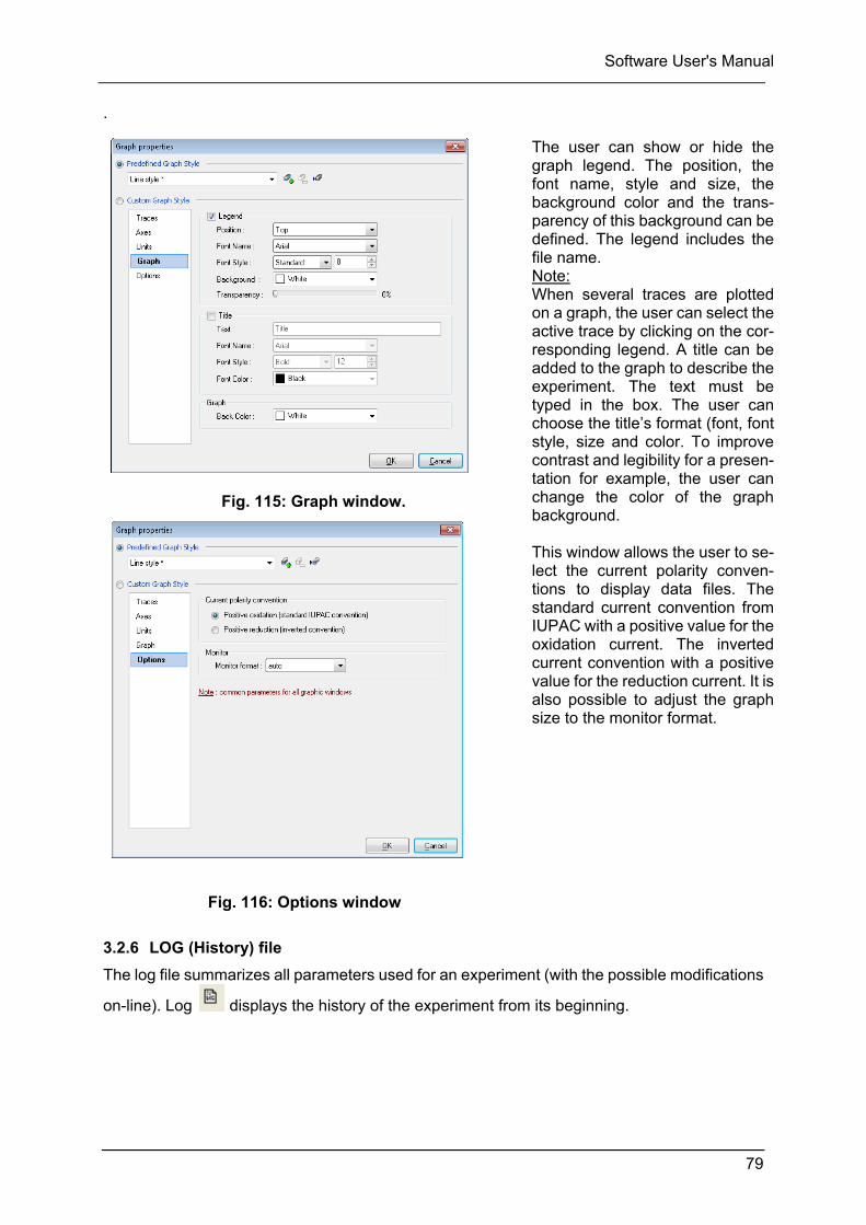
Software User's Manual
79
.
Fig. 116: Options window
3.2.6 LOG (History) file
The log file summarizes all parameters used for an experiment (with the possible modifications
on-line). Log displays the history of the experiment from its beginning.
Fig. 115: Graph window.
The user can show or hide the graph legend. The position, the font name, style and size, the background color and the trans-parency of this background can be defined. The legend includes the file name. Note: When several traces are plotted on a graph, the user can select the active trace by clicking on the cor-responding legend. A title can be added to the graph to describe the experiment. The text must be typed in the box. The user can choose the title’s format (font, font style, size and color. To improve contrast and legibility for a presen-tation for example, the user can change the color of the graph background.
. This window allows the user to se-lect the current polarity conven-tions to display data files. The standard current convention from IUPAC with a positive value for the oxidation current. The inverted current convention with a positive value for the reduction current. It is also possible to adjust the graph size to the monitor format.
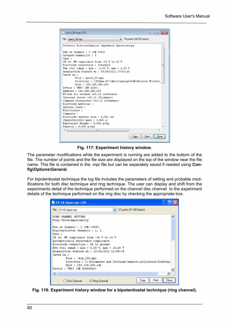
Software User's Manual
80
Fig. 117: Experiment history window.
The parameter modifications while the experiment is running are added to the bottom of the file. The number of points and the file size are displayed on the top of the window near the file name. This file is contained in the .mpr file but can be separately saved if needed using Con-fig\Options\General. For bipotentiostat technique the log file includes the parameters of setting and probable mod-ifications for both disc technique and ring technique. The user can display and shift from the experiments detail of the technique performed on the channel disc channel to the experiment details of the technique performed on the ring disc by checking the appropriate box.
Fig. 118: Experiment history window for a bipotentiostat technique (ring channel).
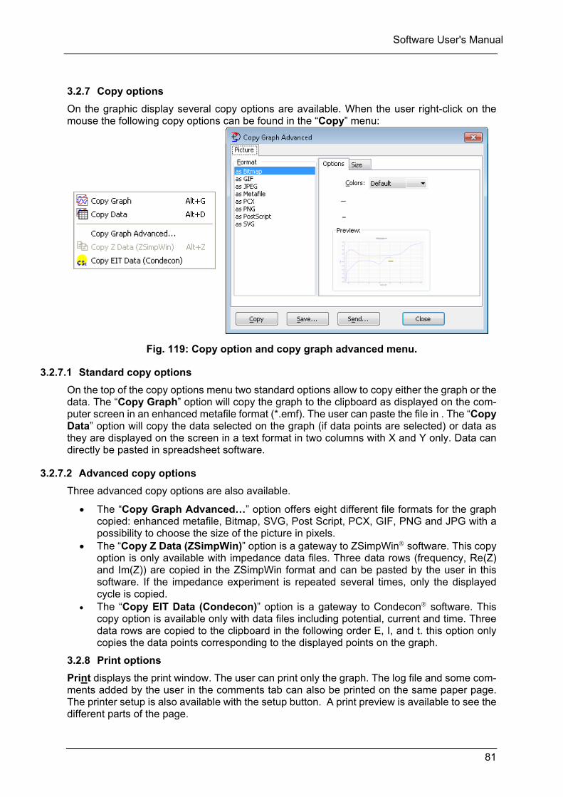
Software User's Manual
81
3.2.7 Copy options
On the graphic display several copy options are available. When the user right-click on the mouse the following copy options can be found in the “Copy” menu:
Fig. 119: Copy option and copy graph advanced menu.
3.2.7.1 Standard copy options
On the top of the copy options menu two standard options allow to copy either the graph or the data. The “Copy Graph” option will copy the graph to the clipboard as displayed on the com-puter screen in an enhanced metafile format (*.emf). The user can paste the file in . The “Copy Data” option will copy the data selected on the graph (if data points are selected) or data as they are displayed on the screen in a text format in two columns with X and Y only. Data can directly be pasted in spreadsheet software.
3.2.7.2 Advanced copy options
Three advanced copy options are also available.
The “Copy Graph Advanced…” option offers eight different file formats for the graph copied: enhanced metafile, Bitmap, SVG, Post Script, PCX, GIF, PNG and JPG with a possibility to choose the size of the picture in pixels.
The “Copy Z Data (ZSimpWin)” option is a gateway to ZSimpWin software. This copy option is only available with impedance data files. Three data rows (frequency, Re(Z) and Im(Z)) are copied in the ZSimpWin format and can be pasted by the user in this software. If the impedance experiment is repeated several times, only the displayed cycle is copied.
The “Copy EIT Data (Condecon)” option is a gateway to Condecon software. This copy option is available only with data files including potential, current and time. Three data rows are copied to the clipboard in the following order E, I, and t. this option only copies the data points corresponding to the displayed points on the graph.
3.2.8 Print options
Print displays the print window. The user can print only the graph. The log file and some com-ments added by the user in the comments tab can also be printed on the same paper page. The printer setup is also available with the setup button. A print preview is available to see the different parts of the page.
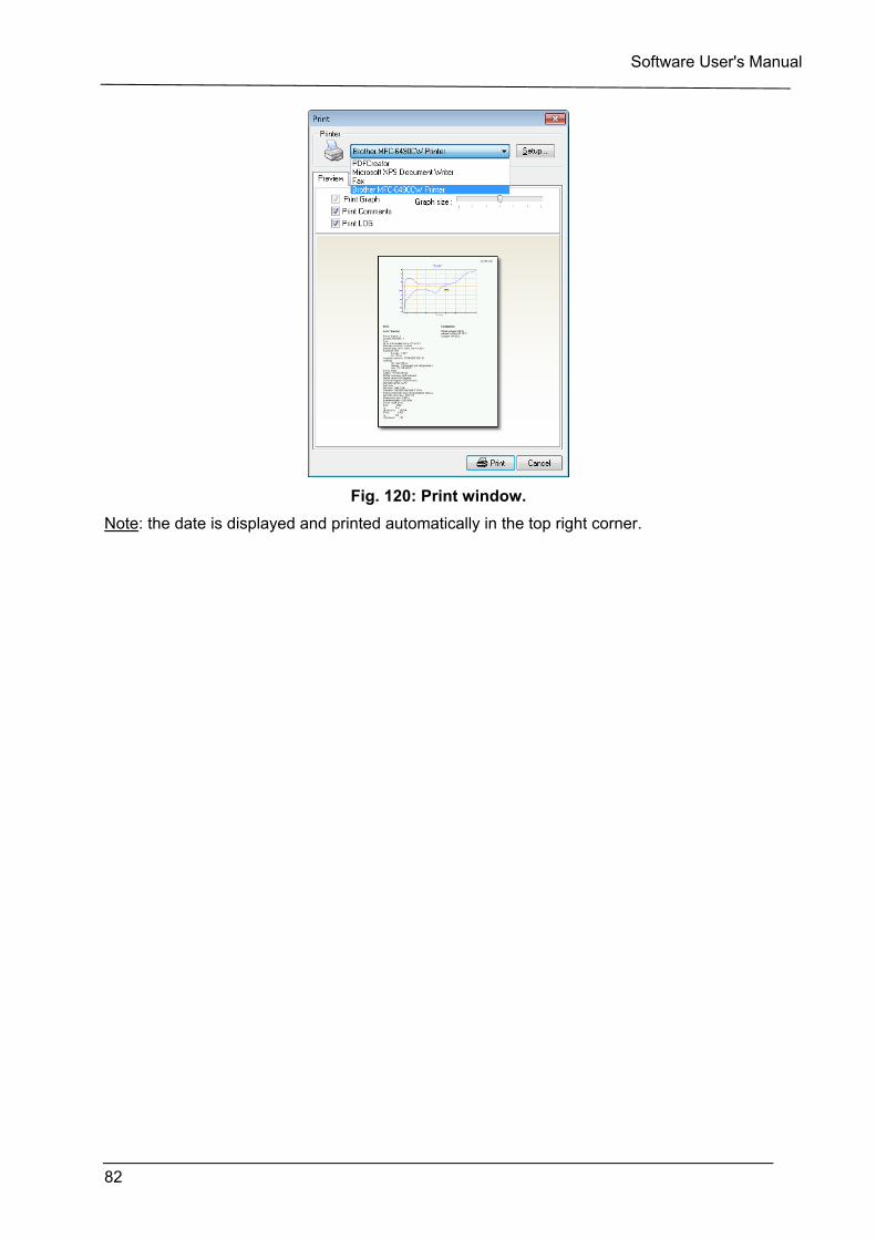
Software User's Manual
82
Fig. 120: Print window.
Note: the date is displayed and printed automatically in the top right corner.
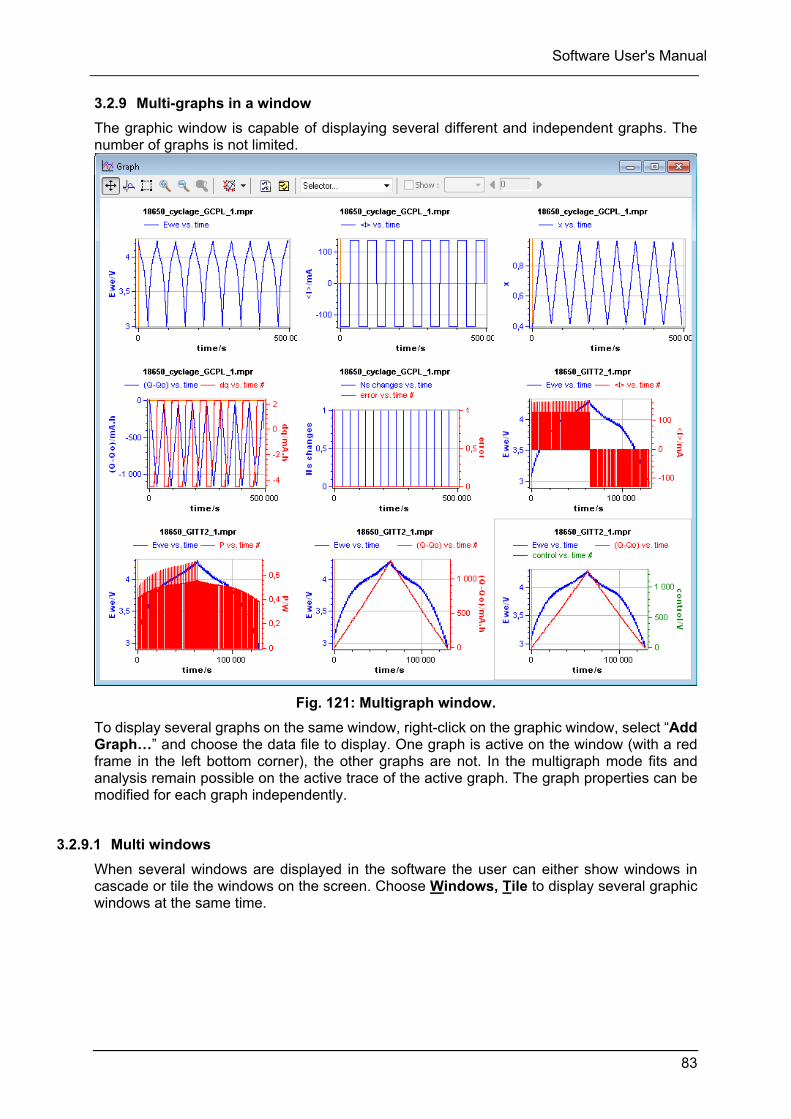
Software User's Manual
83
3.2.9 Multi-graphs in a window
The graphic window is capable of displaying several different and independent graphs. The number of graphs is not limited.
Fig. 121: Multigraph window.
To display several graphs on the same window, right-click on the graphic window, select “Add Graph…” and choose the data file to display. One graph is active on the window (with a red frame in the left bottom corner), the other graphs are not. In the multigraph mode fits and analysis remain possible on the active trace of the active graph. The graph properties can be modified for each graph independently.
3.2.9.1 Multi windows
When several windows are displayed in the software the user can either show windows in cascade or tile the windows on the screen. Choose Windows, Tile to display several graphic windows at the same time.
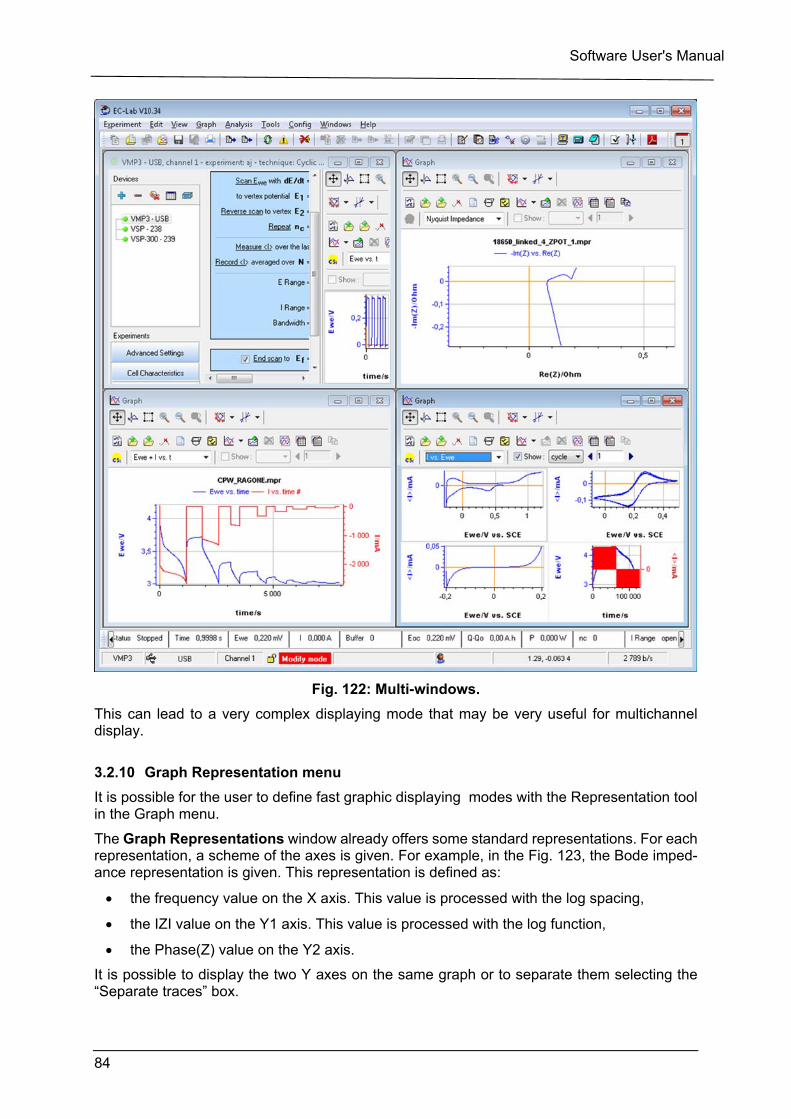
Software User's Manual
84
Fig. 122: Multi-windows.
This can lead to a very complex displaying mode that may be very useful for multichannel display.
3.2.10 Graph Representation menu
It is possible for the user to define fast graphic displaying modes with the Representation tool in the Graph menu.
The Graph Representations window already offers some standard representations. For each representation, a scheme of the axes is given. For example, in the Fig. 123, the Bode imped-ance representation is given. This representation is defined as:
the frequency value on the X axis. This value is processed with the log spacing,
the IZI value on the Y1 axis. This value is processed with the log function,
the Phase(Z) value on the Y2 axis.
It is possible to display the two Y axes on the same graph or to separate them selecting the “Separate traces” box.
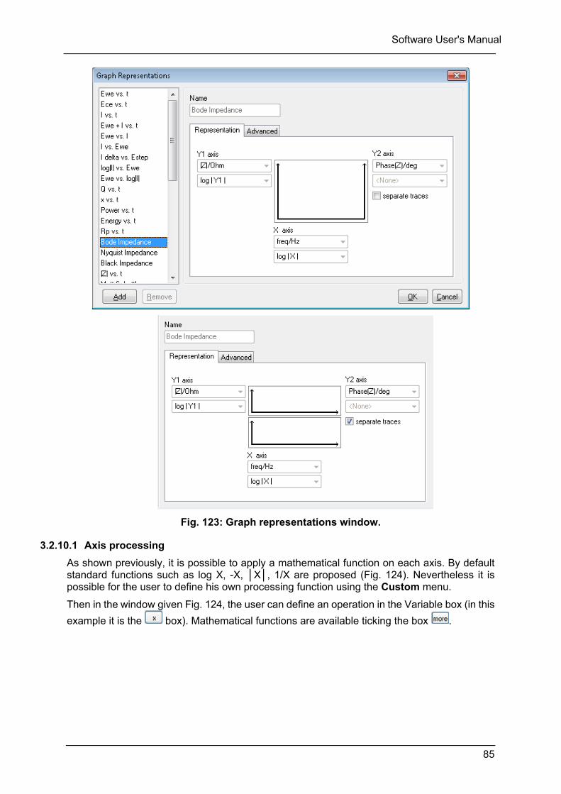
Software User's Manual
85
Fig. 123: Graph representations window.
3.2.10.1 Axis processing
As shown previously, it is possible to apply a mathematical function on each axis. By default standard functions such as log X, -X, X, 1/X are proposed (Fig. 124). Nevertheless it is possible for the user to define his own processing function using the Custom menu.
Then in the window given Fig. 124, the user can define an operation in the Variable box (in this
example it is the box). Mathematical functions are available ticking the box .
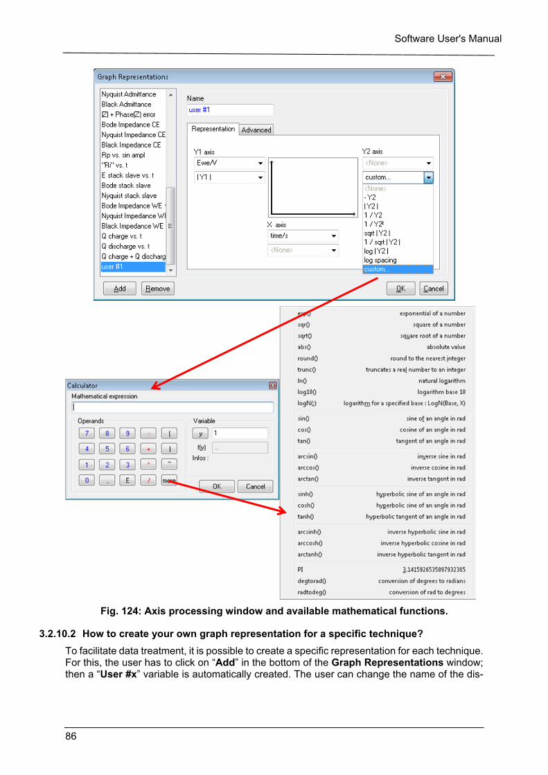
Software User's Manual
86
Fig. 124: Axis processing window and available mathematical functions.
3.2.10.2 How to create your own graph representation for a specific technique?
To facilitate data treatment, it is possible to create a specific representation for each technique. For this, the user has to click on “Add” in the bottom of the Graph Representations window; then a “User #x” variable is automatically created. The user can change the name of the dis-
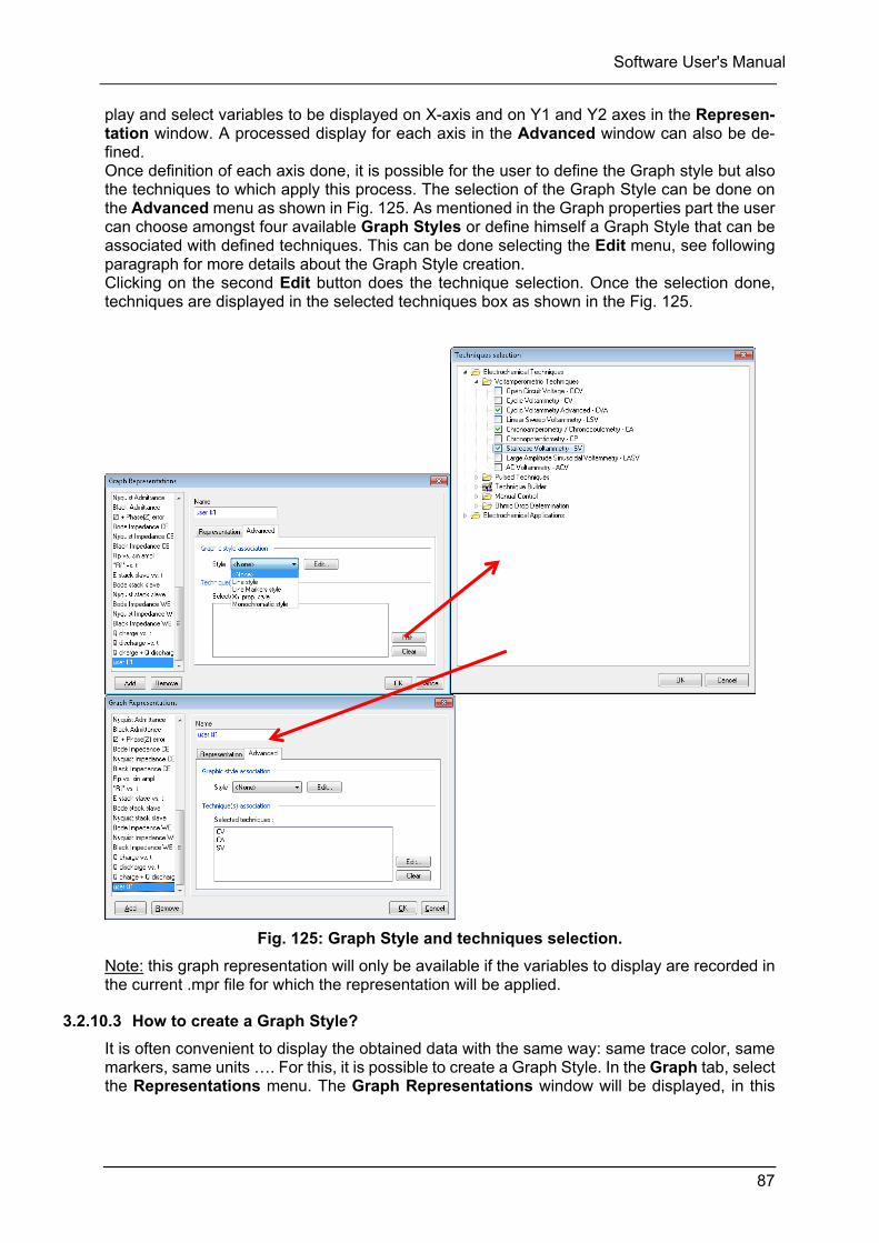
Software User's Manual
87
play and select variables to be displayed on X-axis and on Y1 and Y2 axes in the Represen-tation window. A processed display for each axis in the Advanced window can also be de-fined. Once definition of each axis done, it is possible for the user to define the Graph style but also the techniques to which apply this process. The selection of the Graph Style can be done on the Advanced menu as shown in Fig. 125. As mentioned in the Graph properties part the user can choose amongst four available Graph Styles or define himself a Graph Style that can be associated with defined techniques. This can be done selecting the Edit menu, see following paragraph for more details about the Graph Style creation. Clicking on the second Edit button does the technique selection. Once the selection done, techniques are displayed in the selected techniques box as shown in the Fig. 125.
Fig. 125: Graph Style and techniques selection.
Note: this graph representation will only be available if the variables to display are recorded in the current .mpr file for which the representation will be applied.
3.2.10.3 How to create a Graph Style?
It is often convenient to display the obtained data with the same way: same trace color, same markers, same units …. For this, it is possible to create a Graph Style. In the Graph tab, select the Representations menu. The Graph Representations window will be displayed, in this
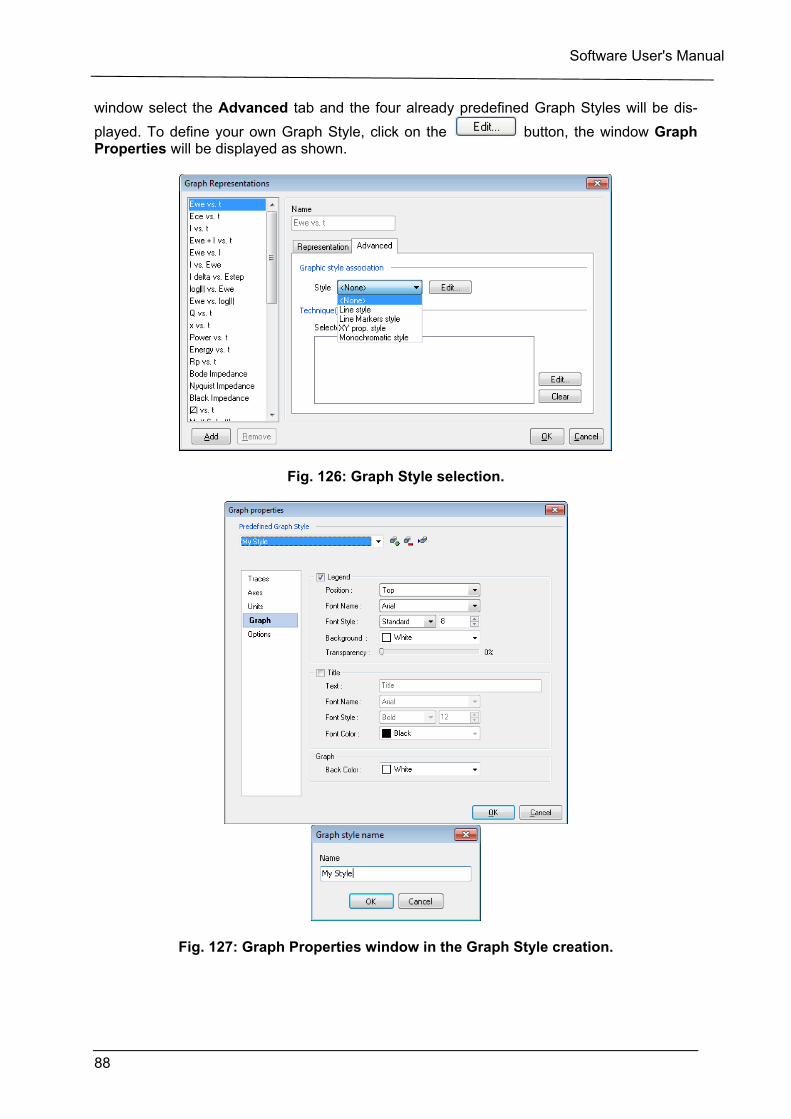
Software User's Manual
88
window select the Advanced tab and the four already predefined Graph Styles will be dis-
played. To define your own Graph Style, click on the button, the window Graph Properties will be displayed as shown.
Fig. 126: Graph Style selection.
Fig. 127: Graph Properties window in the Graph Style creation.
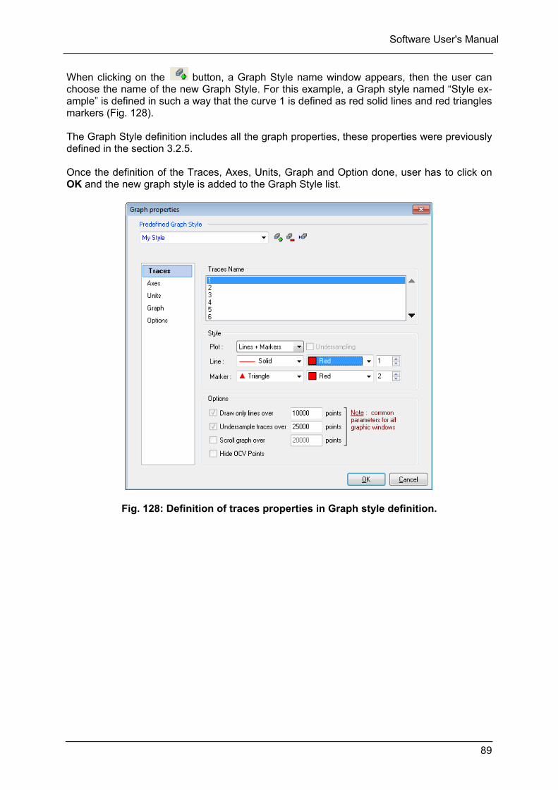
Software User's Manual
89
When clicking on the button, a Graph Style name window appears, then the user can choose the name of the new Graph Style. For this example, a Graph style named “Style ex-ample” is defined in such a way that the curve 1 is defined as red solid lines and red triangles markers (Fig. 128). The Graph Style definition includes all the graph properties, these properties were previously defined in the section 3.2.5. Once the definition of the Traces, Axes, Units, Graph and Option done, user has to click on OK and the new graph style is added to the Graph Style list.
Fig. 128: Definition of traces properties in Graph style definition.
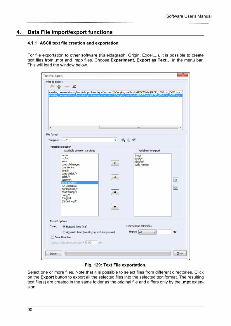
Software User's Manual
90
4. Data File import/export functions
4.1.1 ASCII text file creation and exportation
For file exportation to other software (Kaleidagraph, Origin, Excel,...), it is possible to create text files from .mpr and .mpp files. Choose Experiment, Export as Text… in the menu bar. This will load the window below.
Fig. 129: Text File exportation.
Select one or more files. Note that it is possible to select files from different directories. Click on the Export button to export all the selected files into the selected text format. The resulting text file(s) are created in the same folder as the original file and differs only by the .mpt exten-sion.
Software User's Manual
91
Several text formats can be created by the software depending on the importing software. For time files one can display the relative time from the beginning of the experiment e.g. t = 0 s for the first point (Elapsed Time (in s) option, default) or the absolute time in year, month, day, hours, minutes and seconds format (Absolute Time (mm/dd/yyyy hh/mm.ss.sss option). It is possible to pick up only the variables of interest with the arrows between the two boxes and modify the position of the variables with the bleu on the right side of the “Variables to Export box”. While running experiment, it is possible to export files. To do so, the user must check the Text export option into the "Cell Characteristics" window before starting the experiment. In that case, the template cannot be selected i.e. all the variable are saved in the mpt file. Loops / cycles text exportation: If the selected file contains linked experiments loops or the cycle number variable (processed files only), then one can export specific loops or cycles. Proceed in the same way as with the Selector: check Same selection for all files if you want to apply the loop/cycle selection to all the selected files. If unchecked, each selected file will have its own loop/cycle selection. Select loop or cycles (if present) with the Export box and edit the selection list with the following rules: - separate each single item by a ';' : <item1>;<item2>;<item3>;... - use '-' to generate a list of consecutive items : <first item>-<last item>;... The example above: '1;3' will select the cycles number 1, and 3. Once the loops or cycles have been selected the text exportation will create one file per loop or cycle selected with the loop or cycle number added to the text file. Note: the user can copy data in text format. Right-click with the mouse and select copy data. The displayed variables will be copied to the clipboard.
4.1.1.1 Template
Some templates are already available in the list. Customized template can be added.
4.1.2 ASCII text file importation from other electrochemical software
The software allows the user to load every text file generated by other electrochemical soft-ware. All text formats can be loaded directly from the “Load data file” function in the Experi-ment menu. If the software recognizes the data file, EC-Lab/BT-Lab® will be able to open it directly. If not the user can import the text file with the “Import from text” function in the Ex-periment menu. This can be done either automatically when it is possible (the format is known by the software) or manually with a definition by the user of the number of columns and of each variable.
In the “Experiment” menu select “Import from text…” or click on the import icon to dis-play the following window:
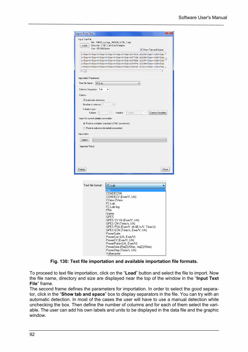
Software User's Manual
92
Fig. 130: Text file importation and available importation file formats.
To proceed to text file importation, click on the “Load” button and select the file to import. Now the file name, directory and size are displayed near the top of the window in the “Input Text File” frame. The second frame defines the parameters for importation. In order to select the good separa-tor, click in the “Show tab and space” box to display separators in the file. You can try with an automatic detection. In most of the cases the user will have to use a manual detection while unchecking the box. Then define the number of columns and for each of them select the vari-able. The user can add his own labels and units to be displayed in the data file and the graphic window.

Software User's Manual
93
Then click on the “Import” button to import the file into the .mpr format. The mpr file is created in the same folder as the text file. Several details are displayed when the file is created such as the name, the number of points and the size. Finally the user can display the .mpr file quickly and easily with the “Display” button. Every analysis is available with the new generated files.
4.1.3 Append file.
This function available in the “Tool” menu allow the user to merge two files. More info 2.7.3.
4.1.4 FC-Lab data files importation
FC-Lab data files can also be imported and analyzed using the “Text file format” function. The FC-Lab data file format is particular as all the data files for each technique are in the same file. So the software will separate every file of every technique used in the experiment.
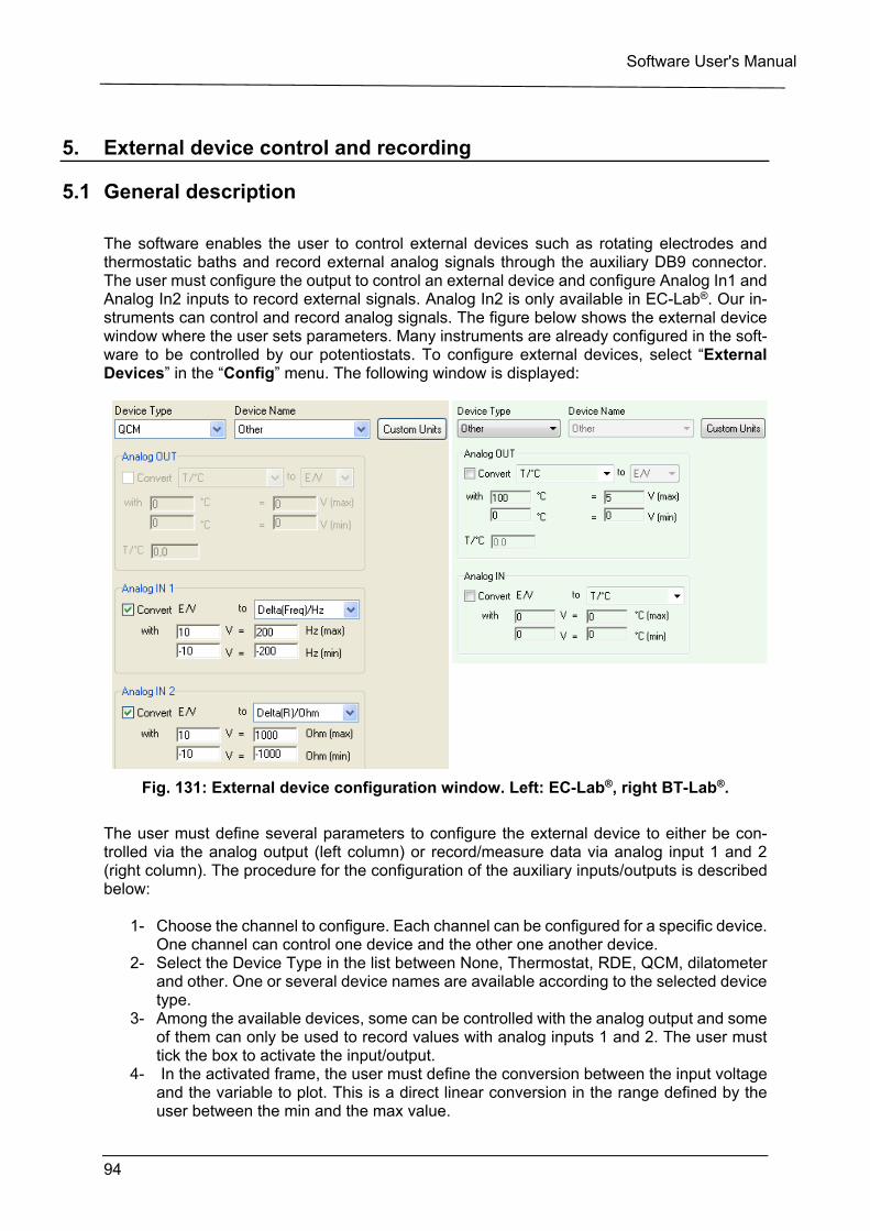
Software User's Manual
94
5. External device control and recording
5.1 General description
The software enables the user to control external devices such as rotating electrodes and thermostatic baths and record external analog signals through the auxiliary DB9 connector. The user must configure the output to control an external device and configure Analog In1 and Analog In2 inputs to record external signals. Analog In2 is only available in EC-Lab®. Our in-struments can control and record analog signals. The figure below shows the external device window where the user sets parameters. Many instruments are already configured in the soft-ware to be controlled by our potentiostats. To configure external devices, select “External Devices” in the “Config” menu. The following window is displayed:
Fig. 131: External device configuration window. Left: EC-Lab®, right BT-Lab®.
The user must define several parameters to configure the external device to either be con-trolled via the analog output (left column) or record/measure data via analog input 1 and 2 (right column). The procedure for the configuration of the auxiliary inputs/outputs is described below:
1- Choose the channel to configure. Each channel can be configured for a specific device. One channel can control one device and the other one another device.
2- Select the Device Type in the list between None, Thermostat, RDE, QCM, dilatometer and other. One or several device names are available according to the selected device type.
3- Among the available devices, some can be controlled with the analog output and some of them can only be used to record values with analog inputs 1 and 2. The user must tick the box to activate the input/output.
4- In the activated frame, the user must define the conversion between the input voltage and the variable to plot. This is a direct linear conversion in the range defined by the user between the min and the max value.
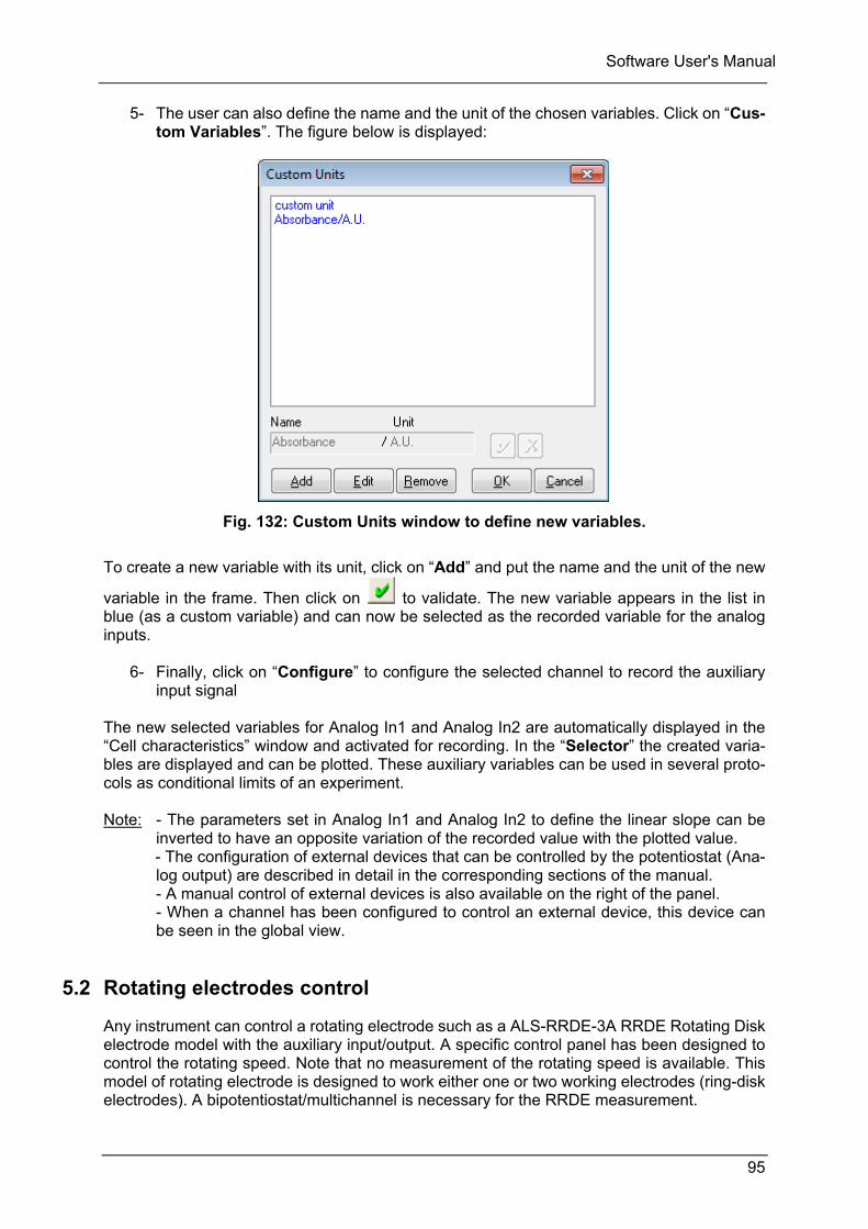
Software User's Manual
95
5- The user can also define the name and the unit of the chosen variables. Click on “Cus-tom Variables”. The figure below is displayed:
Fig. 132: Custom Units window to define new variables.
To create a new variable with its unit, click on “Add” and put the name and the unit of the new
variable in the frame. Then click on to validate. The new variable appears in the list in blue (as a custom variable) and can now be selected as the recorded variable for the analog inputs.
6- Finally, click on “Configure” to configure the selected channel to record the auxiliary input signal
The new selected variables for Analog In1 and Analog In2 are automatically displayed in the “Cell characteristics” window and activated for recording. In the “Selector” the created varia-bles are displayed and can be plotted. These auxiliary variables can be used in several proto-cols as conditional limits of an experiment. Note: - The parameters set in Analog In1 and Analog In2 to define the linear slope can be
inverted to have an opposite variation of the recorded value with the plotted value. - The configuration of external devices that can be controlled by the potentiostat (Ana-log output) are described in detail in the corresponding sections of the manual.
- A manual control of external devices is also available on the right of the panel. - When a channel has been configured to control an external device, this device can be seen in the global view.
5.2 Rotating electrodes control
Any instrument can control a rotating electrode such as a ALS-RRDE-3A RRDE Rotating Disk electrode model with the auxiliary input/output. A specific control panel has been designed to control the rotating speed. Note that no measurement of the rotating speed is available. This model of rotating electrode is designed to work either one or two working electrodes (ring-disk electrodes). A bipotentiostat/multichannel is necessary for the RRDE measurement.
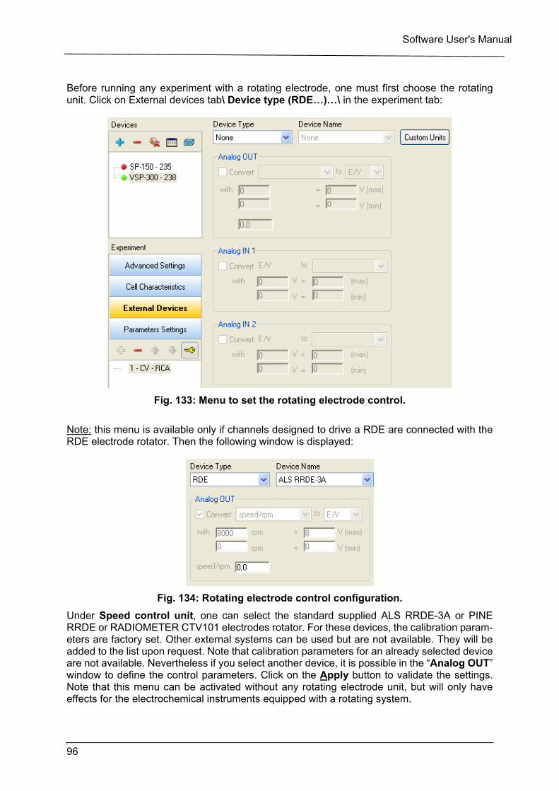
Software User's Manual
96
Before running any experiment with a rotating electrode, one must first choose the rotating unit. Click on External devices tab\ Device type (RDE…)…\ in the experiment tab:
Fig. 133: Menu to set the rotating electrode control.
Note: this menu is available only if channels designed to drive a RDE are connected with the RDE electrode rotator. Then the following window is displayed:
Fig. 134: Rotating electrode control configuration.
Under Speed control unit, one can select the standard supplied ALS RRDE-3A or PINE RRDE or RADIOMETER CTV101 electrodes rotator. For these devices, the calibration param-eters are factory set. Other external systems can be used but are not available. They will be added to the list upon request. Note that calibration parameters for an already selected device are not available. Nevertheless if you select another device, it is possible in the “Analog OUT” window to define the control parameters. Click on the Apply button to validate the settings. Note that this menu can be activated without any rotating electrode unit, but will only have effects for the electrochemical instruments equipped with a rotating system.
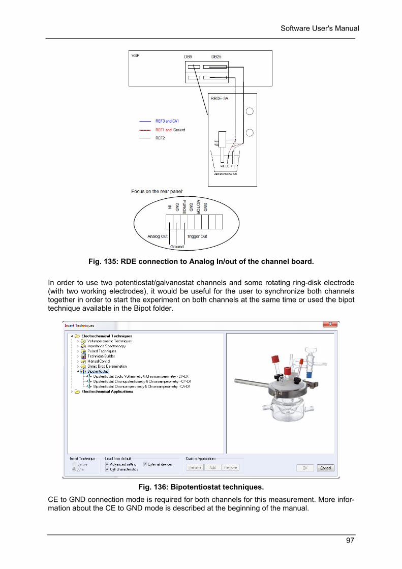
Software User's Manual
97
Fig. 135: RDE connection to Analog In/out of the channel board.
In order to use two potentiostat/galvanostat channels and some rotating ring-disk electrode (with two working electrodes), it would be useful for the user to synchronize both channels together in order to start the experiment on both channels at the same time or used the bipot technique available in the Bipot folder.
Fig. 136: Bipotentiostat techniques.
CE to GND connection mode is required for both channels for this measurement. More infor-mation about the CE to GND mode is described at the beginning of the manual.
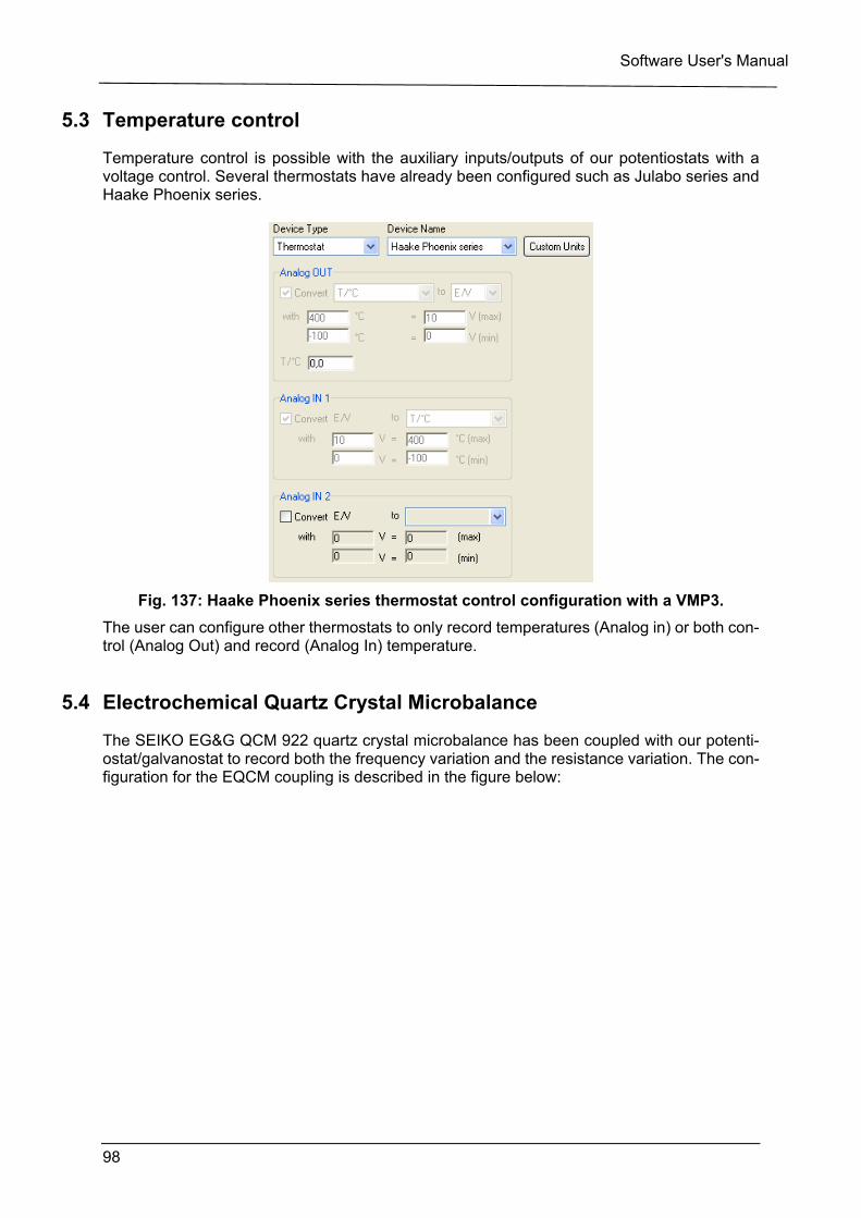
Software User's Manual
98
5.3 Temperature control
Temperature control is possible with the auxiliary inputs/outputs of our potentiostats with a voltage control. Several thermostats have already been configured such as Julabo series and Haake Phoenix series.
Fig. 137: Haake Phoenix series thermostat control configuration with a VMP3.
The user can configure other thermostats to only record temperatures (Analog in) or both con-trol (Analog Out) and record (Analog In) temperature.
5.4 Electrochemical Quartz Crystal Microbalance
The SEIKO EG&G QCM 922 quartz crystal microbalance has been coupled with our potenti-ostat/galvanostat to record both the frequency variation and the resistance variation. The con-figuration for the EQCM coupling is described in the figure below:
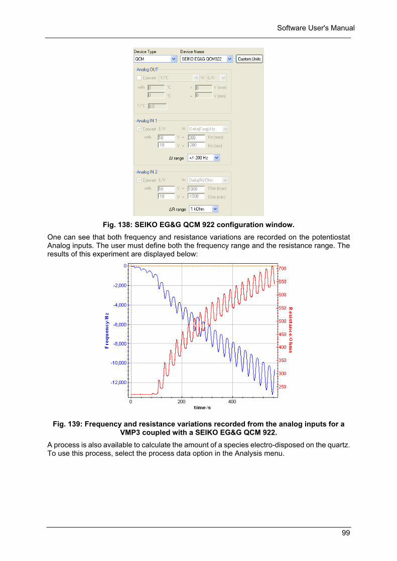
Software User's Manual
99
Fig. 138: SEIKO EG&G QCM 922 configuration window.
One can see that both frequency and resistance variations are recorded on the potentiostat Analog inputs. The user must define both the frequency range and the resistance range. The results of this experiment are displayed below:
Fig. 139: Frequency and resistance variations recorded from the analog inputs for a VMP3 coupled with a SEIKO EG&G QCM 922.
A process is also available to calculate the amount of a species electro-disposed on the quartz. To use this process, select the process data option in the Analysis menu.

Software User's Manual
100
6. Troubleshooting
6.1 In case of problem
Information on your hardware and software configuration is necessary to analyze and finally solve the problem you encounter.
If you have any questions or if any problem occurs that is not mentioned in this document, please contact your local retailer. You can find contact Bio-Logic Instruments or Representative for warranty, service or technical support by click on the following link: http://www.bio-logic.net
Bio-Logic Science Instruments SAS Ph: +33 476 986 831 F: +33 476 986 909 4 rue de Vaucanson 38170 - Seyssinet-Pariset France The highly-qualified staff will be glad to help you. Please keep information on the following at hand:
- Description of the error (the error message, mpr file, picture of setting or any other useful information) and of the context in which the error occurred. Try to remember all steps you had performed immediately before the error oc-curred. The more information on the actual situation you can provide, the easier it is to track the problem.
- The serial number of the device located on the rear panel device.
- The software and hardware version you are currently using. On the Help menu, click “About”. The displayed dialog box shows the version numbers.
- The operating system on the connected computer. - The connection mode (Ethernet, LAN, USB) between computer and instru-
ment.
Model: VMP3 s/n°: 0001Power: 110-240 Vac 50/60 HzFuses: 10 AF Pmax: 650 W
Software User's Manual
101
6.2 Data saving
Problem: Data cannot be saved from a given channel (this channel appears in yellow into the software and the program displays an error message while attempting to save data): Solution(s): - ensure that the saved file has not be moved, destroyed, opened by another application. - if the saved file is on a network drive, ensure that you have the right to write data into the
same directory (create and destroy a text file). Else see your network authorizations… - in the software select Tools, Repair... Then select the saved file and click on the Repair
button. - ensure that the computer IP Address has not been modified since the beginning of the
experiment. - if the problem persists, contact us.
6.3 PC Disconnection
Problem: The PC is disconnected from the instrument ("Disconnected" is displayed in red on the software status bar): Solution(s): - check the PC – instrument connection:
- direct connection: verify that the crossed Ethernet cable is plugged from both ends. - network connection: verify that the yellow led is blinking on the instrument front panel
and that you can access to your network directories from the PC. - check that the green LED is blinking (this assumes that the multichannel potentiostat is
always running properly). - in the Tera Term Pro window type "r" or "R" : this will restart the Ethernet connection pro-
gram that is a part of the instrument firmware. WARNING: this operation is not a simple task, so proceed like this only in case of trouble.
- if the problem persists, contact us.
6.4 Effect of computer save options on data recording
Electrochemical experiments can often have a long duration (more than 24 hours). During the experiment, the computer should always be able to record the data points. If the user enables the power save option for his hard disk, data saving can be disabled. In order to avoid this, we advise the user to remove the power save option from the computer in the settings panel.
Software User's Manual
102
7. Glossary
This glossary is made to help the user understand most of the terms of the software and the terms mentioned in the manual. The terms are defined in the alphabetical order. Absolute value: mathematical function that changes the negative values in positive ones. Accept: button that switches to "Modify" when the user clicks on. "Modify" must be displayed to run the experiment. Booster: current power booster that can be added to each channel individually. Apparent resistance (Ri): conventional term defining the electrolytic resistance in a solid elec-trochemical system such as a battery. Ri is defined as the ratio dE/dI when the potentiostat switches from an open circuit voltage mode to galvanostatic mode and vice versa. ASCII file exportation: exportation of the raw data files or the processed data files to ASCII text format in order to use them with other software (new format: .mpt). Axis: graphic function used to define the axis range, the logarithmic spacing and the grid lines. Bandwidth: represents the frequency of the regulation loop of the potentiostat. It depends on the electrochemical cell impedance. The bandwidth’s values go from 1 to 9. BT-Lab: software drives the battery cyclers. Calibration: operation that must be done for each channel in order to reduce the difference between a controlled value (for example Ectrl) and the corresponding measured value (for ex-ample Ewe). Capacity per cycle: processing function that calculates the capacity per cycle for the gal-vanostatic with potential limitation, the chronocoulometry / chronoamperometry, the cyclic volt-ammetry, and the potentiodynamic cycling with galvanostatic acceleration protocols. CASP Fit: tool available with the graphic display used to fit a curve obtained with the Constant Amplitude Sinusoidal microPolarization technique. This tool is used to determine the current corrosion and the coefficients of corrosion. Channels: each one of the boards corresponding to an independent potentiostat/galvanostat. Characteristic mass: total mass of the species in the electrochemical cell in most of the cases. It is different from the mass of electroactive material. This mass is used in the graphic display to represent mass current density, or mass charge density. Circle Fit: tool available with the graphic display used to fit a circular curve. Compact: mathematical function allowing the user to compress data points from the raw data file. Compact functions are available with the GCPL and PCGA protocols. All points of each potential step are replaced by their average taken at the end of the potential step. The number of points of the compacted data file decreases a lot compared to the raw file.
Software User's Manual
103
Compliance: correspond to the potential range of the counter electrode versus the working electrode potential. This option is used in molten salt electrochemistry where the potential de-creases a lot between the counter and the reference electrode. CE to ground connection: also called N'Stat connection, this mode allows the user to lead measurements on eight working electrodes with one or eight reference electrodes and one counter electrode connected to the ground. It is a very useful tool for biosensors study. This mode can be activated in the "Advanced settings" window. Corr. Sim.: this tool simulates corrosion curves obtained with the linear polarization, Constant Amplitude Sinusoidal microPolarization or Variable Amplitude Sinusoidal microPolarization techniques. Cycle: inside a protocol, this term is used to describe a sequence repeated with time. Cycle number: processing function that allows the user to display on the graphic one or sev-eral cycles chosen in the raw file. The selected cycles are lightened and the others are hidden. Cyclic voltammetry (CV): this protocol consists of scanning the potential of the working elec-trode linearly and measuring the current resulting from oxydoreduction reactions. Cyclic volt-ammetry provides information on redox processes, electron transfer reactions, and adsorption processes. Default settings: settings defined and saved as default by the user and automatically opened when the corresponding protocol is selected. Description: tab in the experiment selection window, which describes the chosen protocol. Device: The software window in the "Config" menu used to add new instrument IP address to be connected to the computer. EC-Lab: software drives the multichannel potentiostats/galvanostat. Electrochemical Noise Analysis: this tool is dedicated to analysis corrosion data and to de-termine the electrochemical noise presents on the data. Electrode characteristics: in the "cell characteristics" window, the user can set all parameters about the electrode. Electrode surface area: geometric surface of the working electrode. It is a value that is used to represent current density or charge density. Experiment limits: in the "advanced settings" window, these limits can be used in two different ways and concern potential, current and charge. The first one is to protect the cell against damages. These limits must be higher than the limits set in the experiment. The second way to use these limits is the control potential resolution. It corresponds to smallest potential step that can be made according to the full potential range. File-Export as text: function that converts the raw data file (.mpr) to a text format file (.mpt). The new created file is located in the same directory as the raw file. File-Import as text: function that converts an ASCII file (.txt) created by other software into a raw data file (.mpr). The new created file is located in the same directory as the text file.
Software User's Manual
104
File- Load: the "load" function allows the user to load a data file (.mpr), a settings file (.mps), a linked experiment settings file (.mpls) or a report file. Filter: this filter can be used as off-line filter many times after the experiment but also just after the recording of the data by ticking a box on the Advanced Setting window. Many methods and windows are available. Fit: graphic tool used to determine kinetic or experimental parameters. Fourier Transform: tool used to apply a Fourier transform to recorded data, many windows are available. Global view: The window where all the channels are shown with the user, the experiment, the state (relax, oxidation, reduction), and the booster or low current board. Group: option used in a multichannel mode to start different experiments on the selected chan-nels at the same time. Hint: small box appearing under the box pointed by the mouse. It indicates the min and the max values accepted in the box. I range: current range used in the experiment. It is related to the current resolution. Impedance: defined by the ratio E/I. Info: tab in the graphic display that gives the number of points and the size of the raw data file. Integral: tool available with the graphic display used to integrate curves. IR compensation: in the electrochemical cell, the resistance between the working and the reference electrode produces a potential drop that keeps the working electrode from being at the controlled potential. IR compensation allows the user to set a resistance value to compen-sate the solution resistance. Limits: in the "advanced settings" window, the experiment limits are used in two ways, first to protect the electrochemical cell from damages during the experiment and second for the po-tential control resolution. Linear Fit: tool available with the graphic display used to fit a curve as a straight line. Linear Interpolation: the linear interpolation allows the user to space out regularly each point of the data file. The user can select to interpolate data by a defined number of points or a regular time between each point. Linked experiments: The software offers the ability to link up to ten different experiments with the protocol linker. Linked experiment settings: the user can save the settings of linked experiments as a .mpls file. This allows the user to easily load all the experiment settings. LOG: function of the graphic display that opens the log file (.mpl) containing details and set-tings of the experiment but no data points. Loop: protocol available in the linked experiments and used to repeat one or more experi-ments. It is different from the cycle in an experiment.
Software User's Manual
105
Low current: option providing a sub-pA resolution that can be added to each channel. This option extends the current range down to 1 nA. This option can be added both to standard and Z option channel boards. Min/Max: graphic tool to determine the min and max values on a selected zone of the curve. Modify: button of the main window allowing the user to select a protocol, change the experi-ment parameters (before or during the experiment). This button switches to "Accept" when the user clicks on. Mott-Schottky: graphic display of 1/C2 vs. Ewe curve and corresponding linear fit to determine slope and offset. MultiExponetial Sim: this tool can be used to simulate curves with multiexponential functions. MultiExponetial Fit: this tool can be used to analyze curves with multiexponential functions. Multi pitting statistics: off-line processing function of the MPP and MPSP protocols that gives the mean values and the mean quadratic deviations of the final rest potentials and the pitting potentials obtained from all the channels used in the experiment. N'Stat: connection mode used to work with several working electrodes, one counter and one reference electrode in the same electrochemical cell. This mode must be used with special connections (see the user’s manual). N'Stat box: accessory provided for measurement in the N'Stat mode. This box has been de-signed for multielectrode cell applications to simplify the potentiostat to cell connection. Open Circuit Voltage (OCV): protocol that consists in a period during which no potential or current is applied to the working electrode. The cell is disconnected and only the potential measurement is available. Option: The software window in the "Config" menu used to choose general parameters of the software such as automatic data saving or warning messages. Pause: button of the main window that leads to a suspension of the progress of the protocol and the measurement recording. The cell is disconnected (OCV period). The "Pause" button switches to "Resume" when clicked. Peak analysis: graphic tool used on an I(E) curve to determine the peak current, the peak potential, exchanged charge quantity, and several other parameters. Preconditioning: previous part of the electrochemical experiment that consists of the equilib-rium state establishment, deaeration period, accumulation of electroactive species on the elec-trode surface or pretreatment of the electrode surface.
Process: function made to calculate or extract values of the raw files (.mpr). The new values (in the .mpp file) can be displayed on the graph. The possibilities of processing depend on the protocol used. Please see the description of each protocol in the application part of the user’s manual to know the processed values.
Protocol linker: tool used to link protocols in order to build a complete experiment with or without open circuit period between protocols.

Software User's Manual
106
Record: in each protocol, the command to define the number of points in the data file. The user can define several recording conditions with potential or charge variation (depending on the galvano or potentio mode) and with time frequency. These data recording option reduces the number of points without losing any interesting changes in the curve. Reference electrode: The user can choose a reference electrode in the list or add his own reference electrode. Report: file that can be associated with the data file to add additional information. Rp Fit: tool available with the graphic display used to calculate a polarization resistance. Run: button that starts the experiment. Save data: button in the experiment frame that forces the data transfer of the selected channel buffer. Scan rate: speed of the potential sweep defined with the smallest possible step amplitude. Selector: window in the graphic display allowing the user to load, add or remove a data file from the graph and to choose the axis parameters. Specifications: characteristics of the instrument such as cell control or current and potential measurement. Stern and Geary model: model of corroding systems based on the Tafel equation. Stop: button used to stop the experiment. Style: graphic function used to define the plot style and color. Subtract files: this tool allows the subtraction of two curves, for example to subtract a back-ground from a curve. Summary per protocol and cycle: off-line processing function giving a table off the maximum and minimum charge, current and potential value for each cycle or loop both in the anodic and cathodic side. Synchronize: option used in a multichannel mode to start the same experiment at the same time on all the selected channels. Tafel Fit: tool available with the graphic display used to determine the corrosion current, the corrosion potential and the polarization resistance with a fit. Tafel graph: off-line processing function allowing the user to display on the graph the logarithm of the current (Tafel plot). Technique builder: section of the selection technique window including the tools and tech-niques used to create linked experiments. Triggers: option that allows the instrument to set a trigger out (TTL signal) at experiment start/stop or to wait for an external trigger in to start or stop the run. Units: graphic function used to modify the axis units.

Software User's Manual
107
VASP Fit: tool available with the graphic display used to fit a curve obtained with the Variable Amplitude Sinusoidal microPolarization technique. This tool is used to determine the current corrosion and the coefficients of corrosion. Wave analysis: graphic tool used on curves obtained in a convective regime and returning the limit current and the half wave potential.
Software User's Manual
108
8. Index
Accept/Modify Settings ............................................................................................... 35, 39, 46 Advanced Settings ................................................................................................................. 16 Batch ...................................................................................................................................... 54 Cell Characteristics ................................................................................................................ 26 Characteristic Mass ................................................................................................................ 78 Colors Configuration ............................................................................................................... 62 Column Mode ......................................................................................................................... 36 Comments ........................................................................................................................ 73, 74 Compliance ...................................................................................................................... 17, 22 Copy ................................................................................................................................. 67, 81
Data .............................................................................................................................. 73, 81 EIT Data (Condecon) ......................................................................................................... 81 Graph ................................................................................................................................. 81 Graph Advanced ................................................................................................................ 81 Z Data (ZSimpWin) ............................................................................................................. 81
Custom Application ................................................................................................................ 41 Cycles ..................................................................................................................................... 91
Process .............................................................................................................................. 71 Show .................................................................................................................................. 70
Data File Name ........................................................................................................................... 61 Hide Selected Points .......................................................................................................... 73 Load ................................................................................................................................... 68 Plot ..................................................................................................................................... 66 Save ................................................................................................................................... 58 Selection ............................................................................................................................. 69 Transfer .............................................................................................................................. 61
Electrode Surface Area .................................................................................................... 28, 78 Electrodes Connection ........................................................................................................... 19
+/- 48 V control mode ......................................................................................................... 25 CE to Ground ..................................................................................................................... 24 N’Stat .................................................................................................................................. 19 Standard ....................................................................................................................... 19, 24 WE to Ground ..................................................................................................................... 24
EQCM ..................................................................................................................................... 98 Equivalent Weight .................................................................................................................. 31 Experiment
Modify Settings ................................................................................................................... 46 Next Sequence ................................................................................................................... 46 Next Technique .................................................................................................................. 46 Pause ................................................................................................................................. 45 Run ..................................................................................................................................... 40 Save ................................................................................................................................... 39 Stop .................................................................................................................................... 45
Export As Text .................................................................................................................. 19, 90 ASCII .................................................................................................................................. 90 Cycles/Loops Selection ...................................................................................................... 91 Format ................................................................................................................................ 62
External device SEIKO EG&G QCM 922 ..................................................................................................... 98
Software User's Manual
109
FC-Lab Import file ............................................................................................................................ 93
File Extensions *.fit ...................................................................................................................................... 55 *.mgp .................................................................................................................................. 55 *.mgr ................................................................................................................................... 55 *.mpl ................................................................................................................................... 55 *.mpp .................................................................................................................................. 55 *.mpr ................................................................................................................................... 55 *.mps .................................................................................................................................. 55 *.mpt ................................................................................................................................... 55
File Repair ............................................................................................................................ 101 Filter
Analog ................................................................................................................................ 22 Floating/Grounded Channel ................................................................................................... 22 Flow Charts Mode .................................................................................................................. 36 Global View .............................................................................................................................. 8 Graph ..................................................................................................................................... 66
2D/3D ................................................................................................................................. 75 Graph Menu
Graph Representations ...................................................................................................... 84 Graph Popup Menu ................................................................................................................ 66 Graph Properties .............................................................................................................. 67, 76 High Speed Scan ................................................................................................................... 22 Hint ......................................................................................................................................... 38 Impedance
Stack .................................................................................................................................. 52 Import From Text .............................................................................................................. 68, 91
Separator ............................................................................................................................ 92 Limits ...................................................................................................................................... 18 Linked Techniques ................................................................................................................. 41 LOG (History) file .................................................................................................................... 79 Loop ..................................................................................................................... 20, 42, 71, 91 Main Menu Bar ......................................................................................................................... 9 Multi-Channel Selection
Group ..................................................................................................................... 49, 51, 53 Stack ...................................................................................................................... 49, 51, 53 Synchronize ............................................................................................................ 49, 51, 53
Multi-Device Connection ........................................................................................................ 15 Multi-Graphs ........................................................................................................................... 83 Ohmic Drop Compensation .................................................................................................... 45 Parameters Settings ............................................................................................................... 36 Parameters Settings ............................................................................................................... 33 Point Coordinates ................................................................................................................... 69 Print ........................................................................................................................................ 81 Process
Display ................................................................................................................................ 72 File ...................................................................................................................................... 90 Loops .................................................................................................................................. 71 Mass ................................................................................................................................... 99 Variables ............................................................................................................................ 56
Process Cycles ................................................................................................................................. 71
QCM-922 ................................................................................................................................ 98 Record
Software User's Manual
110
Analog Input ....................................................................................................................... 33 Conditions .................................................................................................................... 38, 57 Ece ..................................................................................................................................... 33 Power ................................................................................................................................. 33
Rotating electrodes ................................................................................................................ 96 Safety Limits ........................................................................................................................... 18 Selector
Add ..................................................................................................................................... 71 Clear ................................................................................................................................... 71 Load ................................................................................................................................... 71 Remove .............................................................................................................................. 71 Undo ................................................................................................................................... 71
Sequences ............................................................................................................................. 38 Settings Popup Menu ............................................................................................................. 34 Smooth ................................................................................................................................... 20 Tool Bars
Channel Selection .............................................................................................................. 13 Configuration ................................................................................................................ 13, 64 Fast Graph Display ............................................................................................................. 84 Fast Graph Selection .................................................................................................... 14, 70 Graph ................................................................................................................................. 70 Lock .................................................................................................................................... 15 Main .................................................................................................................................... 13
Ultra Low Current Option ........................................................................................................ 22 User ........................................................................................................................................ 58 Variables ................................................................................................................................ 56 Virtual Potentiostat ................................................................................................................. 59 Wait ........................................................................................................................................ 42 Warning Messages ................................................................................................................. 61 ZSimpWin ............................................................................................................................... 91
Software User's Manual
111
9. List of Notes
9.1 Application Notes
AN#1 – Protocols for studying intercalation electrodes materials: Part I: Galvanostatic cycling with potential limitation (GCPL)
AN#2 – Protocols for studying intercalation electrodes materials: Part II: Potentiody-namic Cycling with Galvanostatic Acceleration (PCGA)
AN#3 – Galvanostatic Cycling with Potential limitation 4: Low Earth Orbit battery sat-ellite protocol
AN#4 – Potentiostat stability mystery explained
AN#5 – Precautions for good impedance measurements
AN#6 – Constant power technique (updated November 5, 2010)
AN#7 – Application of the bipotentiostat to an experiment with a rotating ring-disk electrode.
AN#8 – Impedance, admittance, Nyquist, Bode, Black, etc…
AN#9 – Linear vs. non linear systems in impedance measurements
AN#10 – Corrosion current measurement for an iron electrode in an acid solution (up-dated February 24, 2011)
AN#11 – Calculation of the platinum’s active surface
AN#12 – UV-Visible Spectroscopy and Electrochemistry coupling: Spectroelectro-chemical experiment feasibility on a polypyrrol film
AN#13 – VMP3 and Quartz Crystal Microbalance coupling: mass measurement dur-ing a polypyrrol film deposition
AN#14 – ZFit and equivalent electrical circuits
AN#15 – Two questions about Kramers-Kronig transformations
AN#16 – Simultaneous Impedance measurements on each element of a running cell stack
AN#17 – Drift correction in electrochemical impedance measurements
AN#18 – Staircase Potentio Electrochemical Impedance Spectroscopy and automatic successive ZFit analysis
AN#19 – EIS measurements with multisine
AN#20 – Pseudo capacitance calculation (updated December 9, 2010)
AN#21 – Measurements of the double layer capacitance
AN#22 – Corrosion of reinforced concrete
AN#23 – EIS measurements on Li-ion batteries – EC-Lab software parameters ad-justment (updated December 9, 2010)
AN#24 – Photovoltaic Characterizations: Polarization and Mott Schottky plot
AN#25 – Multi Pitting Corrosion
AN#26 – Graphic Customization
AN#27 – Ohmic Drop: Part I: Effect on measurements
AN#28 – Ohmic Drop: Part II: Introduction to Ohmic Drop measurement techniques
AN#29 – Ohmic Drop Part III: Suitable use of the ZIR techniques?
AN#30 – IMVS investigation on photovoltaic cell (updated June 8, 2010)
AN#31 – Fuel Cell Testing – Part I: Overview and I/E characterizations
AN#32 – Fuel Cell Testing – Part II: EIS characterization
Software User's Manual
112
AN#33 – Supercapacitors investigations – Part I: Charge/discharge cycling (updated August 28, 2012)
AN#34 – Supercapacitors investigations – Part II: Time constant determination (up-dated May 2, 2014)
AN#35 – Application of the Capacitance-Voltage curve to photovoltaic cell characteri-zations
AN#36 – VASP: An innovative and exclusive technique for corrosion monitoring
AN#37 – CASP: a new method for the determination of corrosion parameters (up-dated October 20, 2011)
AN#38 – Dynamic resistance determination. A relation between AC and DC measure-ments?
AN#39-I – Electrochemical Noise Measurements – Part I : ASTM assessment and validation of the instrumental noise
AN#39-II – Electrochemical Noise Measurements – Part II : ASTM assessment and validation on a real electrochemical system
AN#39-III – Electrochemical Noise Measurements – Part III : Determination of the noise resistance Rn
AN#40 – Differential (Incremental) Capacity Analysis
AN#41-I - CV Sim – Simulation of the simple redox reaction (E) – Part I : The effect of the scan rate
AN#41-II - CV Sim – Simulation of the simple redox reaction (E) – Part II : The effect of the ohmic drop and the double layer capacitance
AN#42 – ZFit : The modified inductance element La.
AN#43 – How to fit transmission lines with ZFit
AN#44 - Artefacts in EIS measurements
AN#45 - Using ZFit for multiple cycles analysis
AN#46 - Dilatometer
AN#47 - Corrosion current determination with mass transfer limitation
AN#48 - Inaccuracy of the corrosion current determination in presence of an ohmic drop: EC-Lab® solutions
AN#49 - EIS measurements: Potentio (PEIS) vs. Galvano (GEIS) mode, that is the question!
AN#50-I - Math Reminder for electrochemists: I. The simplicity of complex number and impedance diagrams
AN#50-II – Math Reminder for electrochemists: II. The simplicity of Laplace transform
AN#51 – Supercapacitor characterization by galvanostatic polarization method – (.pdf 597 Ko)
AN#52 – UFS-SEC: the spectroElectrochemical Cell for UV-Vis, NIR and IR measur-ment – ( .pdf 208 Ko )
AN#53 - Precision and Accuracy in Coulombic Efficiency Measurements (.pdf 654 Ko). Sample data (.mpr 16 Mo).
AN#54 – How to read EIS accuracy contour plots
AN#55 – Interpretation problems of impedance measurements made on time variant systems
AN#56 – Electrochemical reaction kinetics measurement: the Levich and Koutecký-Levich analysis tools
AN#57 – Differential Coulometry Spectroscopy (DCS)
AN#58 – Cycling battery with reference electrode by using the PAT-cell test cell
Software User's Manual
113
AN#59 – A full solution to address battery module/pack.
AN#60 – Distribution of Relaxation Times (DRT): an introduction
AN#61 – How to interpret lower frequencies impedance in batteries?
9.2 Technical Notes
TN 1 – VMP, VMP2, MPG or BiStat IP address change TN 2 – Accessing the VMP, VMP2, MPG or BiStat from other networks through gate-
ways TN 3 – Computer TCP/IP installation and configuration TN 4 – VMP2, VMP or MPG firmware upgrading TN 6 – The Data smooth option (updated February 8, 2010) TN 7 – The “compact” Function in the PCGA protocol TN 8 – Adjustment of the potential control resolution TN 9 – Various connection modes Part I: Ewe vs. Ece control in the standard mode TN 10 – “p” low current option: installation and calibration TN 11 – Other channel to cell connection mode – Part II: CE to Ground mode TN 12 – Low current N’Stat box installation (VMP2, BiStat, VSP, VMP3) TN 13 – Long cell cables TN 17 – Instantaneous versus averaged current measurement TN 18 – Channel board: installation and calibration for VMP2, VMP3, VSP TN 19 – Network parameters configuration with EC-Lab® and EC-Lab® Express
software TN 20 – MEASURE versus CONTROL mode: extended current ranges TN 21 – External device control and recording TN 22 – Graphic properties – Part I: Graph Style definition TN 23 – Graphic properties – Part II: Graph Representation definition TN 24 – Potentiostat board installation on SP-300 chassis (BiPotentiostat option) TN 25a – Control of the potential/current signal by an external device Part I : control
by a Low Frequency Generator (LFG) TN 25b – Control of the potential/current signal by an external device Part II : control
by a channel of the potentiostat TN 26 – How to configure an experiment with a platinum temperature probe? TN 27 – SAM-50 : Module for measurements on stack of 50V TN 28 – EQCM cell Set-up TN 29 – How to use the purge tube? TN 30 – Which GCPL technique is the most appropriate for my measurement? TN 31 – Isolation System IS1 – How and why? TN 32 – How to set the data recording conditions of my measurement? TN 33 – DC-DC boards for SP-300 technology instruments TN 34 – How fast the instrument is able to switch from potentio to galvano mode &
vice versa? TN 35 – Bandwidth selection TN 36 – Boards validation TN 37 – Peristaltic pump Installation TN 38 – BCD technique: Battery Capacity Determination TN 39 – Import urban profile (txt file) TN 40 – Influence of the current range on the response time of a potentiostat TN 41 – Climate Chamber control with EXTAPP