Ecohydrology

Fall 2015Matt Cohen

SFRC

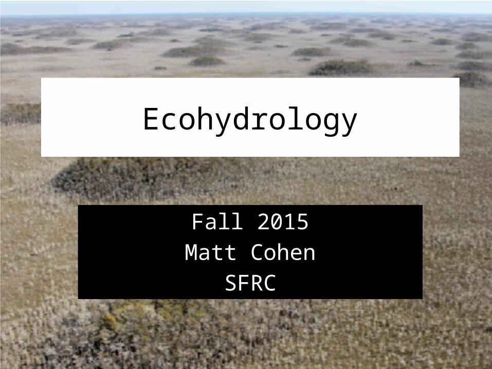
Introductions• Name• Department• Title of your research (thesis, dissertation)• Ecohydrology Ordination

Ecology Hydrology

Theoretical

Applied

MC

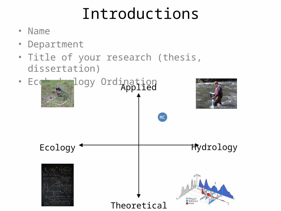
Course Goals

• Study the dynamic and reciprocal interplay between biota and their abiotic environment (broadly construed “hydrology”)

• Develop synthesis skills by focusing a large topic area into a small space [paper]

• Develop hypothesis and analysis skills by addressing a research question [project]

• Develop teaching skills by guiding a group learning experience [discussion]

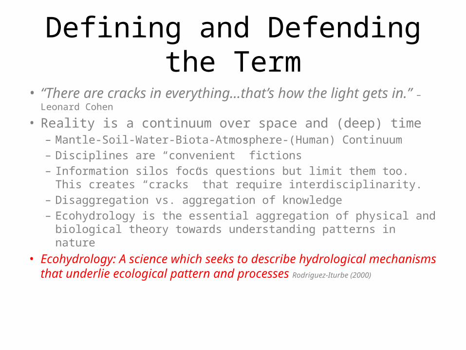
Defining and Defending the Term

• “There are cracks in everything…that’s how the light gets in.” – Leonard Cohen

• Reality is a continuum over space and (deep) time– Mantle-Soil-Water-Biota-Atmosphere-(Human) Continuum– Disciplines are “convenient” fictions – Information silos focus questions but limit them too. This creates

“cracks” that require interdisciplinarity.– Disaggregation vs. aggregation of knowledge– Ecohydrology is the essential aggregation of physical and biological

theory towards understanding patterns in nature• Ecohydrology: A science which seeks to describe hydrological

mechanisms that underlie ecological pattern and processes Rodriguez-Iturbe (2000)

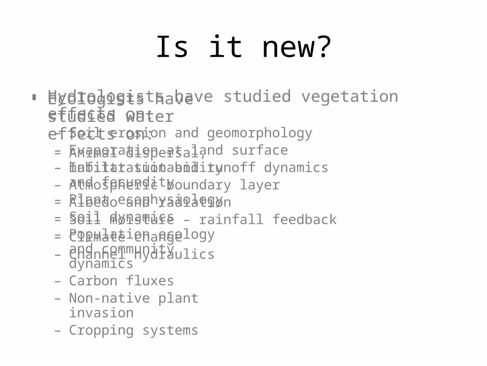
Is it new?

• Ecologists have studied water effects on:– Animal dispersal, habitat

suitability and fecundity– Plant ecophysiology– Soil dynamics – Population ecology and

community dynamics – Carbon fluxes– Non-native plant invasion– Cropping systems

• Hydrologists have studied vegetation effects on:– Soil erosion and geomorphology– Evaporation at land surface– Infiltration and runoff dynamics– Atmospheric boundary layer– Albedo and radiation– Soil moisture – rainfall feedback– Climate change– Channel hydraulics

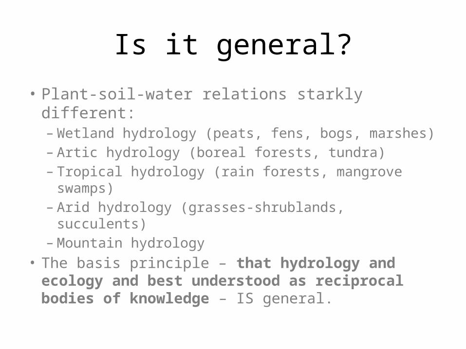
Is it general?

• Plant-soil-water relations starkly different:– Wetland hydrology (peats, fens, bogs, marshes)– Artic hydrology (boreal forests, tundra)– Tropical hydrology (rain forests, mangrove swamps)– Arid hydrology (grasses-shrublands, succulents)– Mountain hydrology

• The basis principle – that hydrology and ecology and best understood as reciprocal bodies of knowledge – IS general.

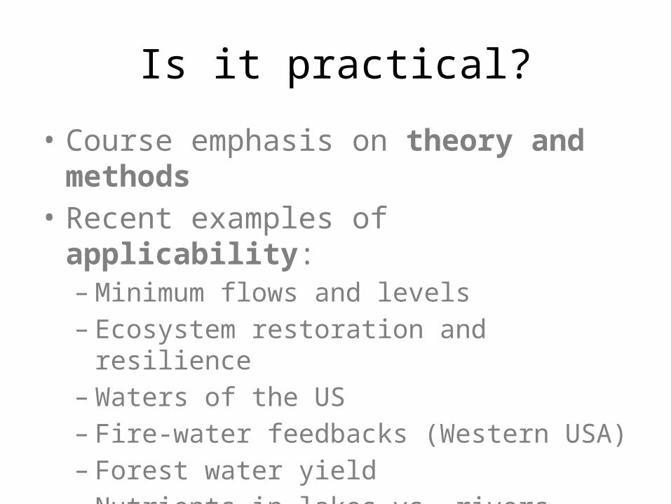
Is it practical?

• Course emphasis on theory and methods• Recent examples of applicability:

– Minimum flows and levels– Ecosystem restoration and resilience– Waters of the US– Fire-water feedbacks (Western USA)– Forest water yield– Nutrients in lakes vs. rivers

Administrative Debris• Instructor: Dr. Matt Cohen

– mjc@ufl.edu– http://sfrc.ufl.edu/ecohydrology/FOR6934.html– Class listserv (TBD)– 352-846-3490– No office hours – by appt. only

• TA: Bobby Hensley– Post-Doc working on springs and aquatic nutrient cycling– bhensley@ufl.edu

• Meeting times– Tuesday: 1:55-2:45 TUR2350, Thursday: 12:50-2:45 TUR2346

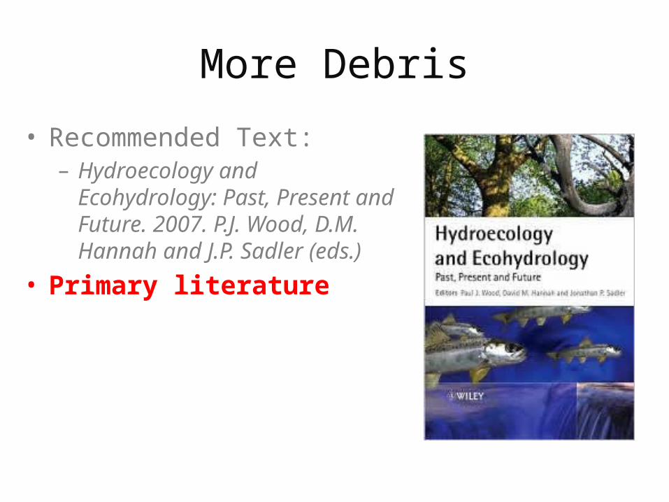
More Debris

• Recommended Text:– Hydroecology and Ecohydrology:

Past, Present and Future. 2007. P.J. Wood, D.M. Hannah and J.P. Sadler (eds.)

• Primary literature

Assignments• Lead class discussion – 25%

– One student each week (except weeks 1 and 2)– Select 1 paper from instructor’s list (more next)

• Everyone gets one week to read this

– Provide background, context, summary, critique• Bring additional literature where necessary

• Synthesis paper – 35%– 15-20 page paper due October 1st.– Topic area selected (with instructor) by Sept. 10th – Synthesis – pick a question with broad scope

Assignments

• Group Research Project – 40%– Proposal due Oct. 8th

• Modest equipment and sample costs can be covered

– Draft manuscripts due Nov. 24th; Final Due Dec. 8th. – Potential subject areas:

• Springs Sediment-Vegetation interactions• Solute variation in Geographically Isolated Wetlands• Soil Moisture Dynamics Across Gradients• Diel River Solute Variation Analysis/Synthesis• Coastal Marsh Salinity Across Gradients

Homework Assignment

• Identify three candidate papers for discussion– One in your area of expertise/focus– One in an area outside your expertise– One synthesis/vision paper

• Send them to the instructor by Thursday. A full list of papers from which you can choose your group discussion lead will follow in ca. 1 week.

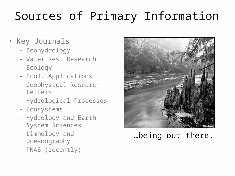
Sources of Primary Information

• Key Journals– Ecohydrology– Water Res. Research– Ecology– Ecol. Applications– Geophysical Research Letters– Hydrological Processes– Ecosystems– Hydrology and Earth System

Sciences– Limnology and Oceanography– PNAS (recently)

…being out there.

Systems Thinking

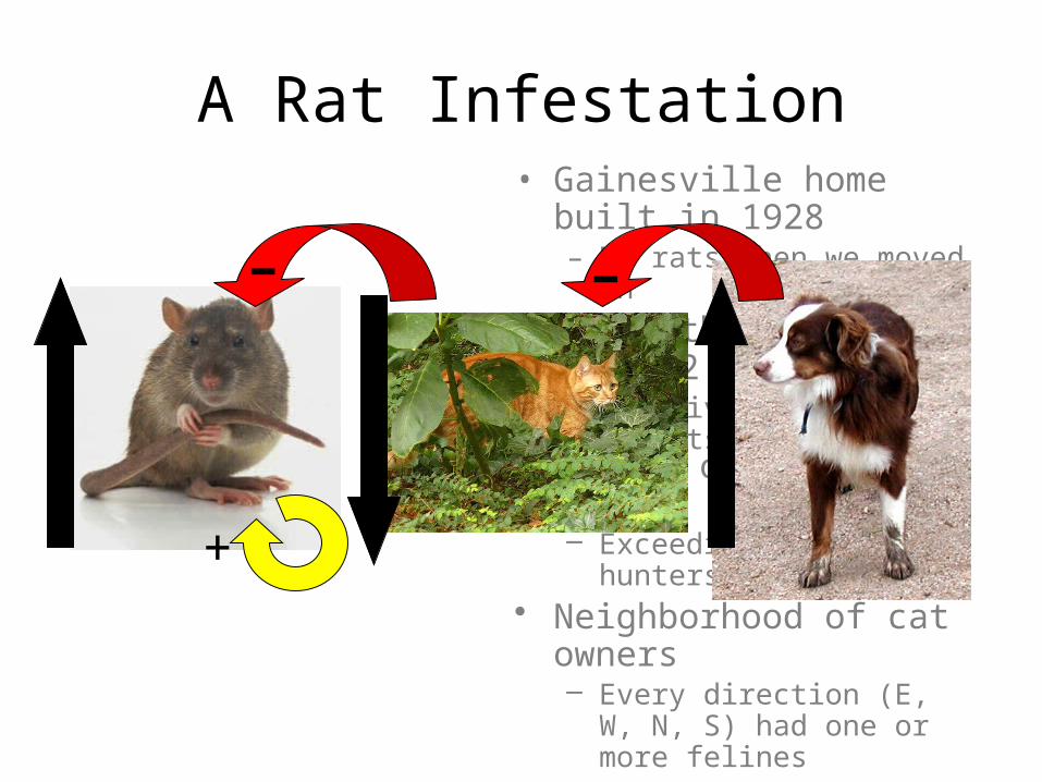
A Rat Infestation• Gainesville home built in 1928

– No rats when we moved in• Lived there for just under 2

years– “Massive” control efforts by the

end

• Owners of 2 large dogs– Exceedingly poor hunters

• Neighborhood of cat owners– Every direction (E, W, N, S) had

one or more felines– Drove the dogs crazy…ever-

vigilant border patrols

+

- -

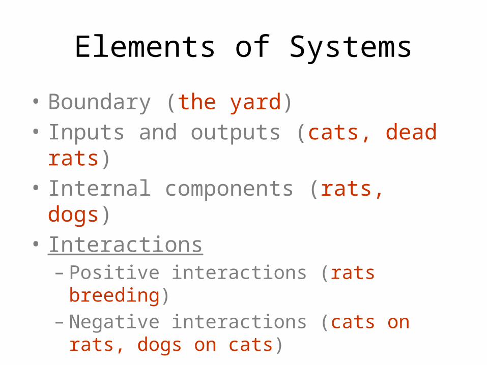
Elements of Systems

• Boundary (the yard)• Inputs and outputs (cats, dead rats)• Internal components (rats, dogs)• Interactions

– Positive interactions (rats breeding)– Negative interactions (cats on rats, dogs on cats)

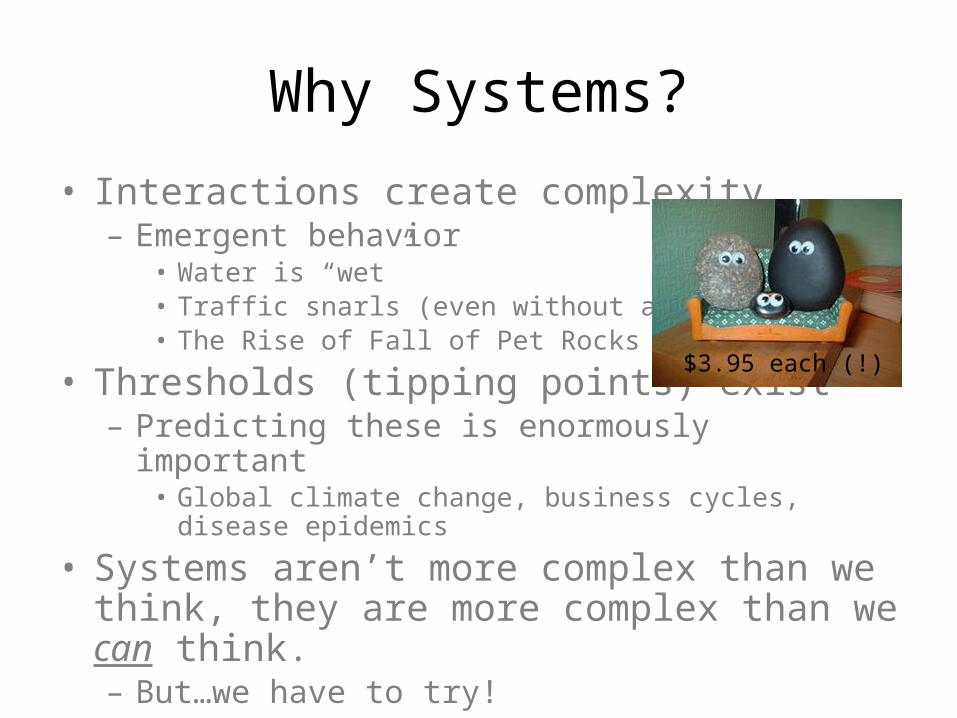
Why Systems?

• Interactions create complexity– Emergent behavior

• Water is “wet”• Traffic snarls (even without accidents)• The Rise of Fall of Pet Rocks

• Thresholds (tipping points) exist– Predicting these is enormously important

• Global climate change, business cycles, disease epidemics

• Systems aren’t more complex than we think, they are more complex than we can think.– But…we have to try!

$3.95 each (!)

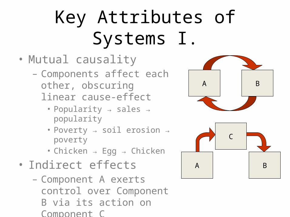
Key Attributes of Systems I.

• Mutual causality– Components affect each other,

obscuring linear cause-effect • Popularity → sales → popularity• Poverty → soil erosion → poverty• Chicken → Egg → Chicken

• Indirect effects– Component A exerts control over

Component B via its action on Component C

A B

A B

C

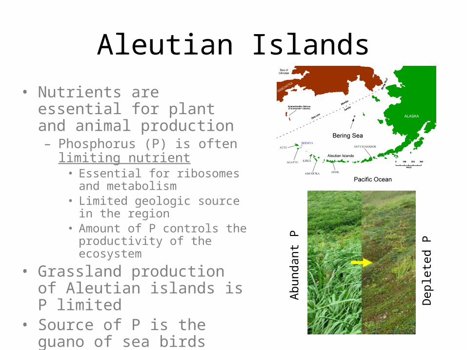
Aleutian Islands• Nutrients are essential for plant

and animal production– Phosphorus (P) is often limiting

nutrient• Essential for ribosomes and

metabolism• Limited geologic source in the

region• Amount of P controls the

productivity of the ecosystem

• Grassland production of Aleutian islands is P limited

• Source of P is the guano of sea birds Ab

unda

nt P

Dep

lete

d P

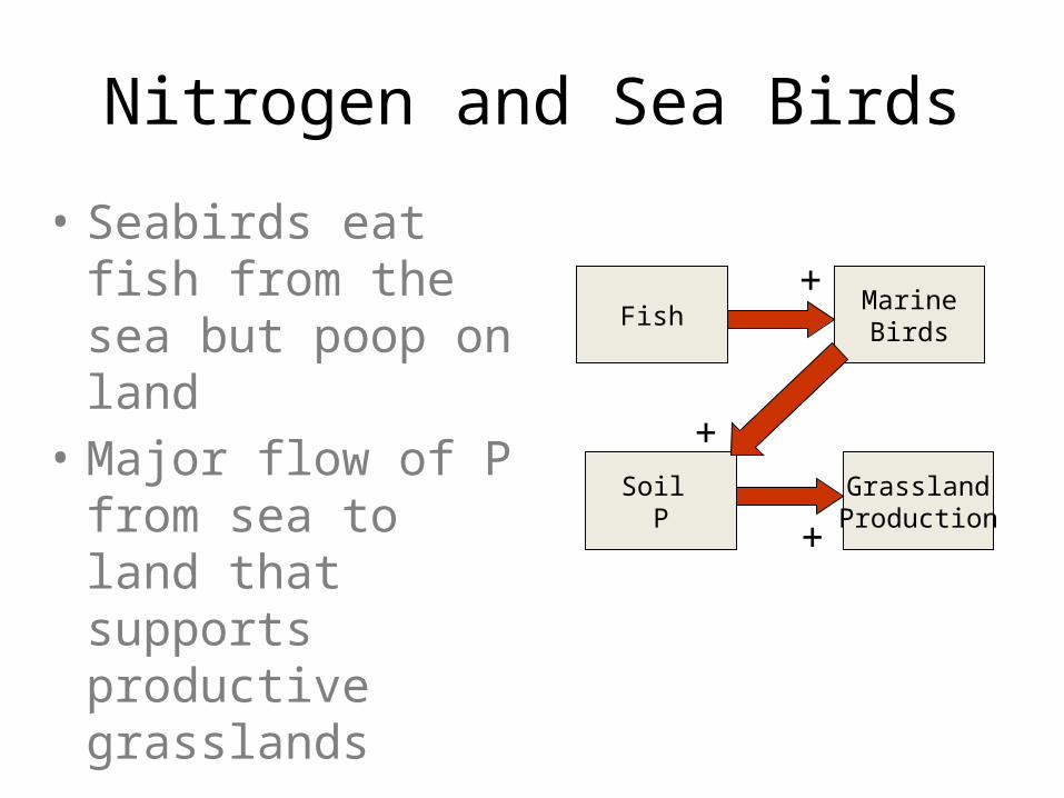
Nitrogen and Sea Birds

• Seabirds eat fish from the sea but poop on land

• Major flow of P from sea to land that supports productive grasslands

MarineBirds

GrasslandProduction

Fish

Soil P

+

+

+

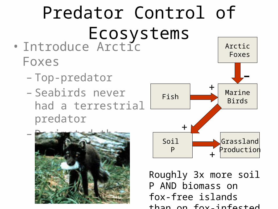
Predator Control of Ecosystems• Introduce Arctic Foxes

– Top-predator– Seabirds never had a

terrestrial predator– Decimated the sea-bird

populations

MarineBirds

GrasslandProduction

Fish

Soil P

+

+

+

Arctic Foxes

-

Roughly 3x more soil P AND biomass on fox-free islands than on fox-infested islands

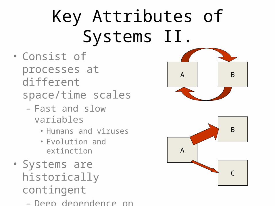
Key Attributes of Systems II.

• Consist of processes at different space/time scales– Fast and slow variables

• Humans and viruses• Evolution and extinction

• Systems are historically contingent– Deep dependence on what

happened in the past• The Great Unfolding• Beta-max, Bacteria, Base 10

A B

A

B

C

Fast & Slow:Time Lags in Complex Systems

• Variables operating at different characteristic “speeds” interact

• Those interactions are complex because they can be affected by delays– Sunburns (anticipating when to reapply)– Hangovers (anticipating when to say “no”)

• This affects natural systems (predator-prey systems) AND economic and social systems (business cycles, shifts in behaviors)

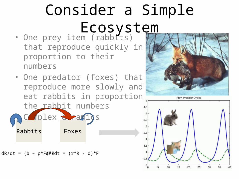
Consider a Simple Ecosystem• One prey item (rabbits) that

reproduce quickly in proportion to their numbers

• One predator (foxes) that reproduce more slowly and eat rabbits in proportion the rabbit numbers

• Complex dynamics

Rabbits Foxes

dR/dt = (b – p*F)*R dF/dt = (r*R - d)*F

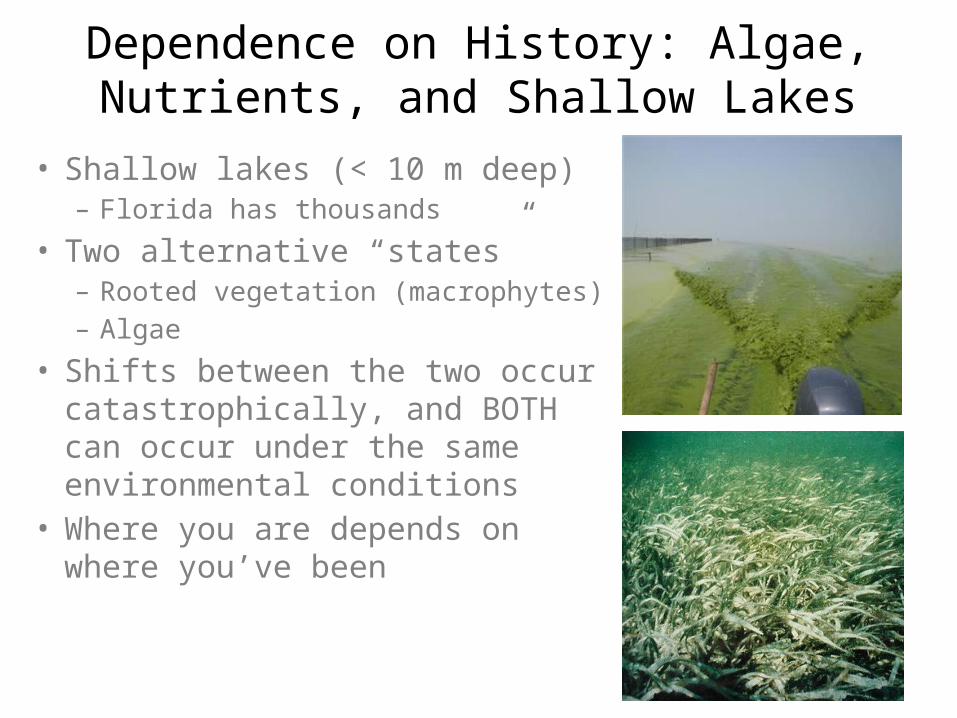
Dependence on History: Algae, Nutrients, and Shallow Lakes

• Shallow lakes (< 10 m deep)– Florida has thousands

• Two alternative “states”– Rooted vegetation (macrophytes)– Algae

• Shifts between the two occur catastrophically, and BOTH can occur under the same environmental conditions

• Where you are depends on where you’ve been

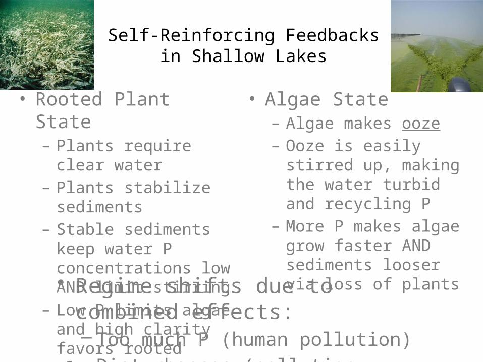
Self-Reinforcing Feedbacks in Shallow Lakes

• Rooted Plant State– Plants require clear water– Plants stabilize sediments– Stable sediments keep

water P concentrations low AND limit stirring

– Low P limits algae and high clarity favors rooted plants

• Algae State– Algae makes ooze– Ooze is easily stirred up,

making the water turbid and recycling P

– More P makes algae grow faster AND sediments looser via loss of plants

• Regime shifts due to combined effects:– Too much P (human pollution)– Disturbances (pollution affects vulnerability)

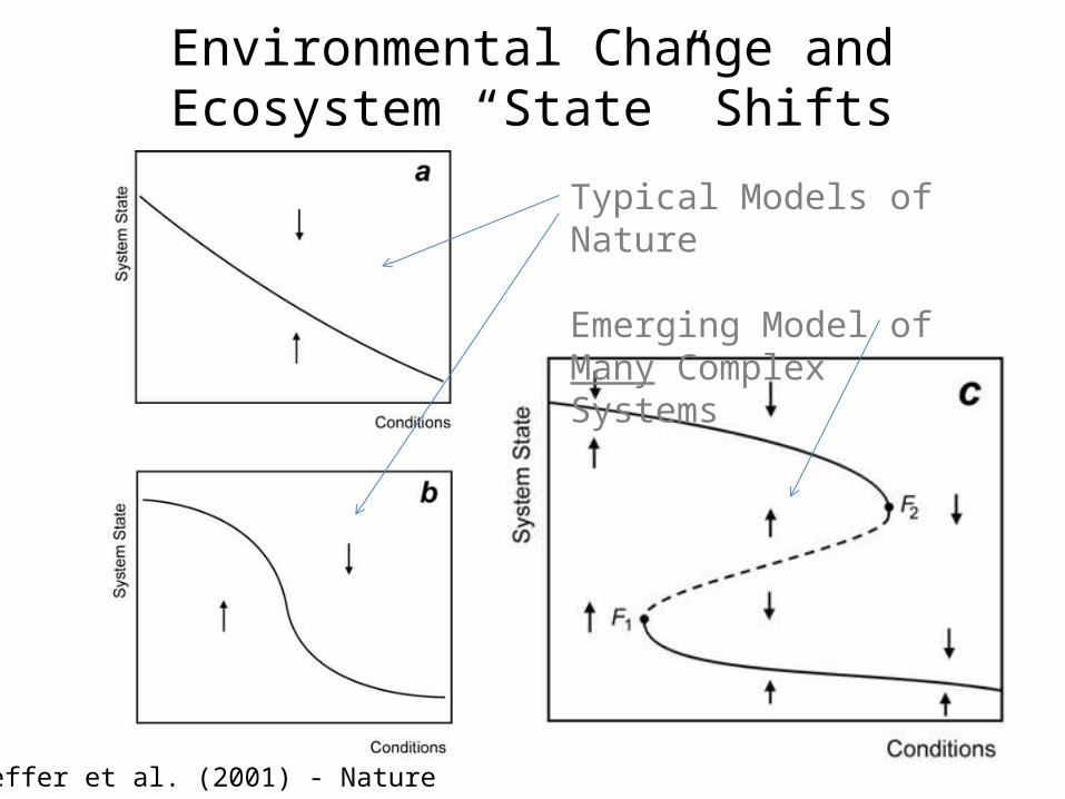
Environmental Change and Ecosystem “State” Shifts

Typical Models of Nature

Emerging Model of Many Complex Systems

Scheffer et al. (2001) - Nature

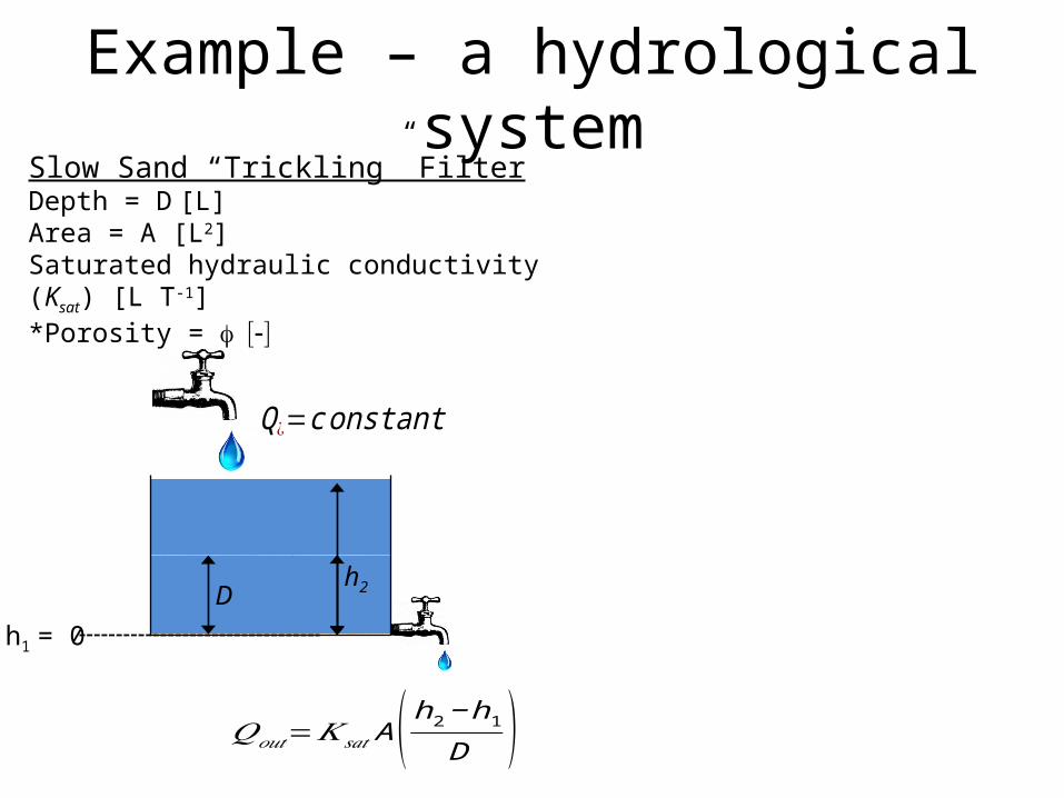
Example – a hydrological system

Slow Sand “Trickling” FilterDepth = D [L]Area = A [L2]Saturated hydraulic conductivity (Ksat) [L T-1]*Porosity = [-]f

𝑄𝑜𝑢𝑡=𝐾 𝑠𝑎𝑡 A ( h2−h1D )

Q¿=c onstant

h2Dh1 = 0

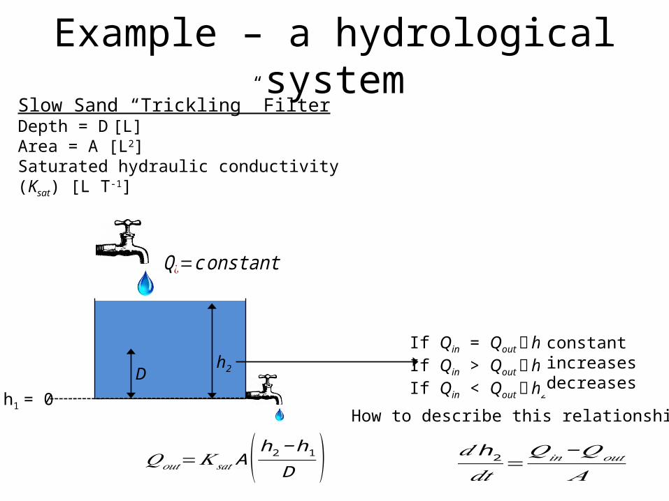
Example – a hydrological system

Slow Sand “Trickling” FilterDepth = D [L]Area = A [L2]Saturated hydraulic conductivity (Ksat) [L T-1]

𝑄𝑜𝑢𝑡=𝐾 𝑠𝑎𝑡 A ( h2−h1D )

Q¿=c onstant

h2Dh1 = 0

If Qin = Qout h2 = ?If Qin > Qout h2 = ?If Qin < Qout h2 = ?

𝑑 h2𝑑𝑡

=𝑄𝑖𝑛−𝑄𝑜𝑢𝑡

𝐴

constantincreasesdecreases

How to describe this relationship?

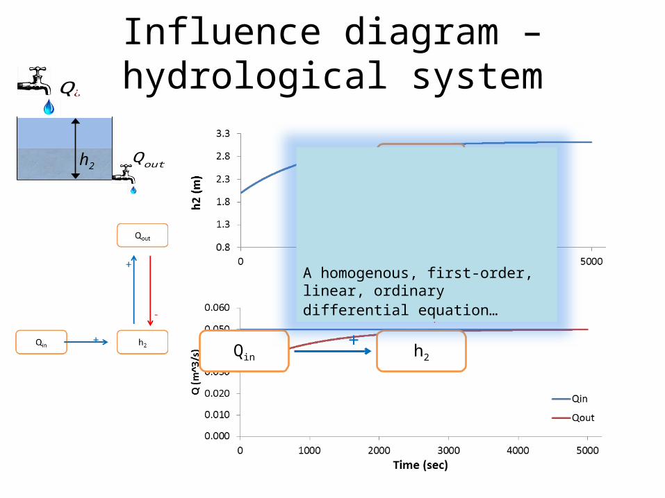
Influence diagram – hydrological system

h2

Q¿

Q out

Qin

Qout

h2+

+

-

A homogenous, first-order, linear, ordinary differential equation…

Example – an ecohydrological system?

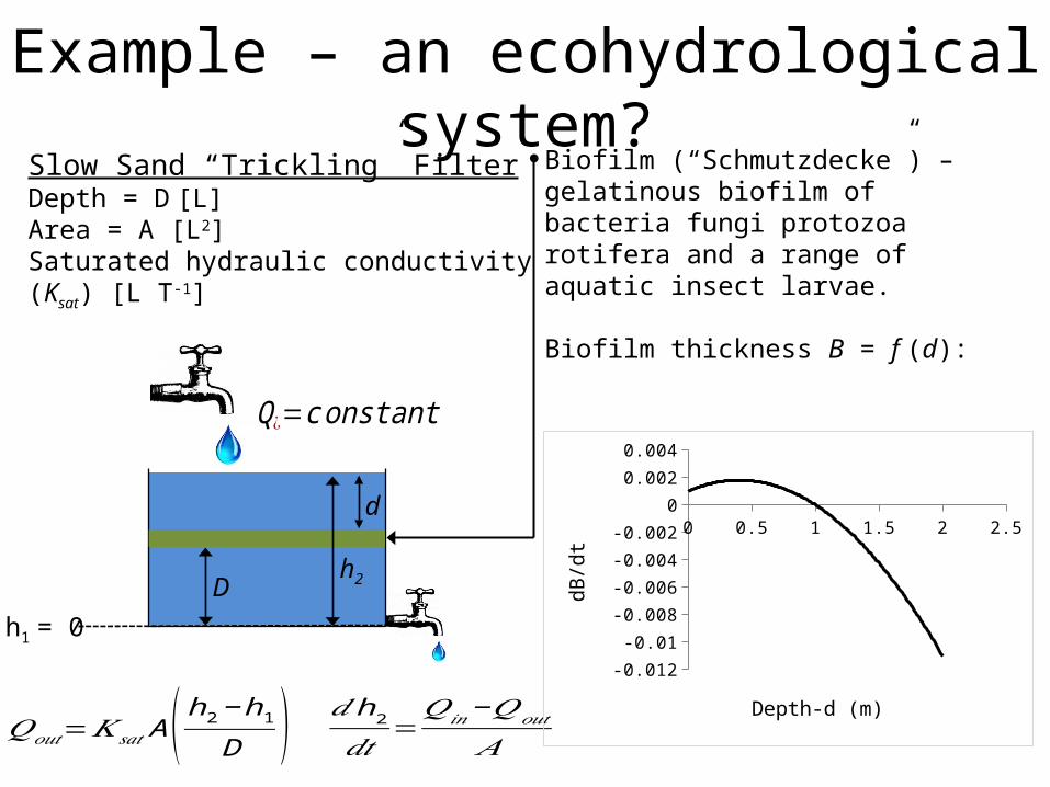
Slow Sand “Trickling” FilterDepth = D [L]Area = A [L2]Saturated hydraulic conductivity (Ksat) [L T-1]

𝑄𝑜𝑢𝑡=𝐾 𝑠𝑎𝑡 A ( h2−h1D )

Q¿=c onstant

h2Dh1 = 0

𝑑 h2𝑑𝑡

=𝑄𝑖𝑛−𝑄𝑜𝑢𝑡

𝐴

Biofilm (“Schmutzdecke”) – gelatinous biofilm of bacteria fungi protozoa rotifera and a range of aquatic insect larvae.

Biofilm thickness B = f (d):

d

0 0.5 1 1.5 2 2.5

-0.012

-0.01

-0.008

-0.006

-0.004

-0.002

0

0.002

0.004

Depth-d (m)

dB/d

t

Example – an ecohydrological system?

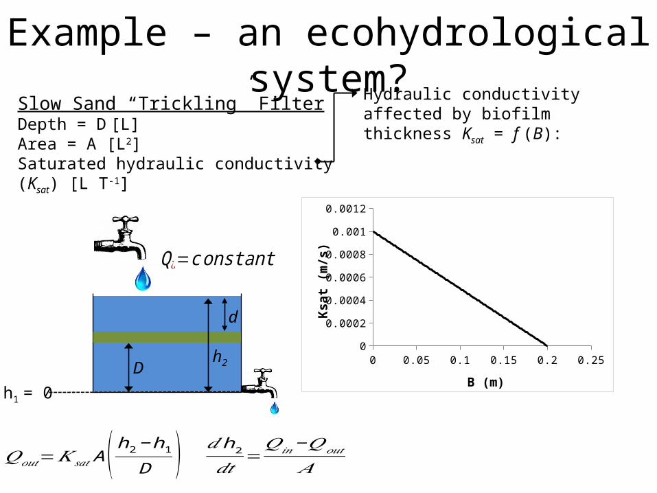
Slow Sand “Trickling” FilterDepth = D [L]Area = A [L2]Saturated hydraulic conductivity (Ksat) [L T-1]

𝑄𝑜𝑢𝑡=𝐾 𝑠𝑎𝑡 A ( h2−h1D )

Q¿=c onstant

h2Dh1 = 0

𝑑 h2𝑑𝑡

=𝑄𝑖𝑛−𝑄𝑜𝑢𝑡

𝐴

d

Hydraulic conductivity affected by biofilm thickness Ksat = f (B):

0 0.05 0.1 0.15 0.2 0.250

0.0002

0.0004

0.0006

0.0008

0.001

0.0012

B (m)

Ksat

(m/s

)

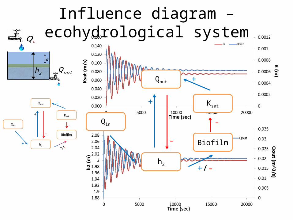
Influence diagram – ecohydrological system

h2

Q¿

Q out

Qin

Qout

h2

Biofilm

Ksat

+

+

-

+

-

+/-

Ecohydrology Examples to Animate Systems Concepts

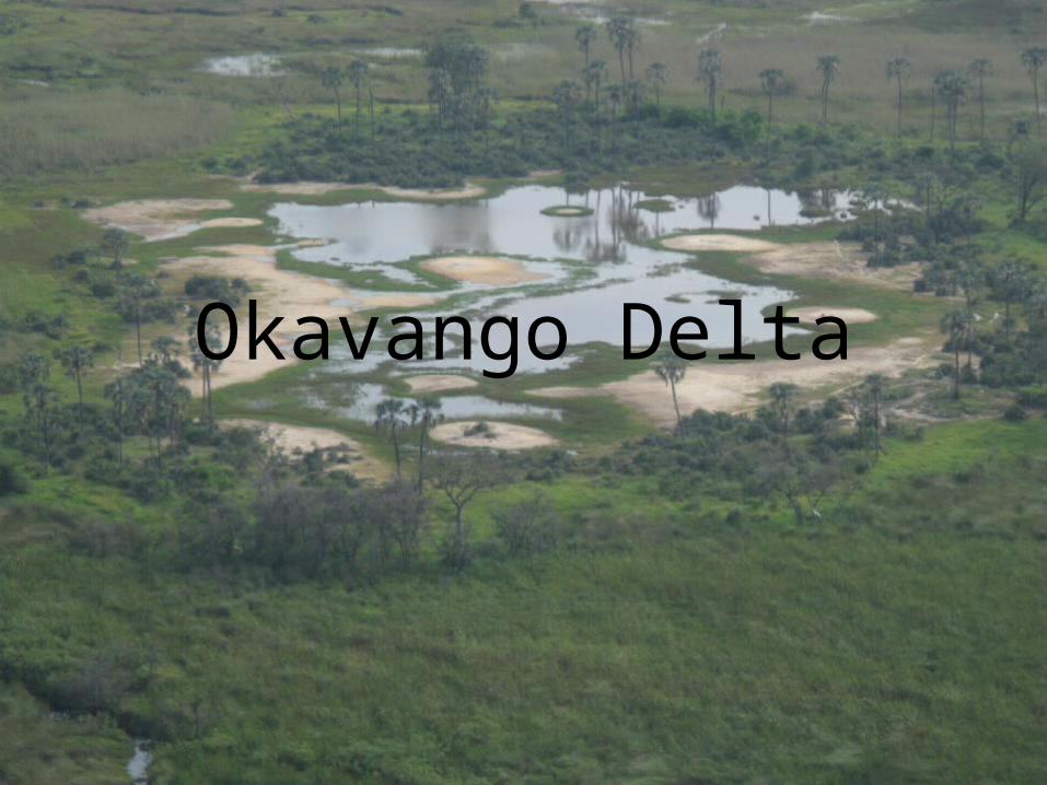
Okavango Delta

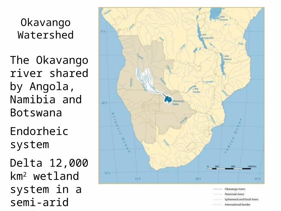
Okavango Watershed

The Okavango river shared by Angola, Namibia and Botswana

Endorheic system

Delta 12,000 km2 wetland system in a semi-arid environment

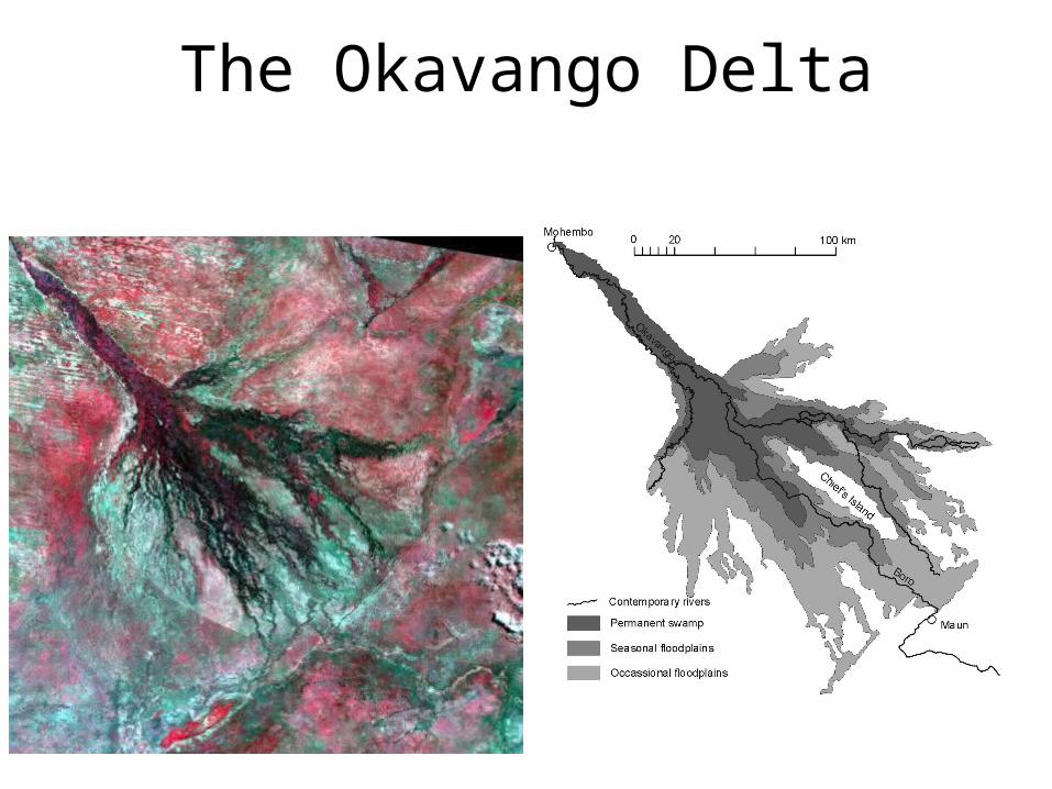
The Okavango Delta

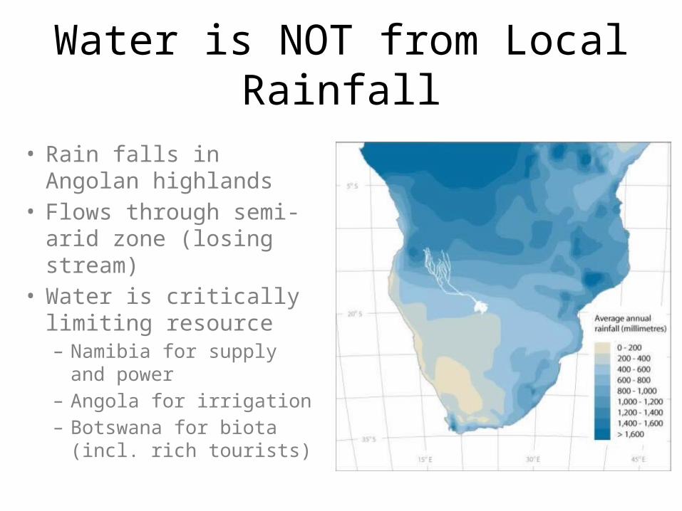
Water is NOT from Local Rainfall

• Rain falls in Angolan highlands

• Flows through semi-arid zone (losing stream)

• Water is critically limiting resource– Namibia for supply and

power– Angola for irrigation– Botswana for biota (incl.

rich tourists)

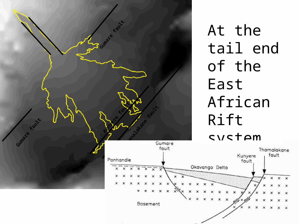
Gumar

e fau

lt

Kunyer

e fau

ltTh

anala

kane f

ault

Gumar

e fau

lt At the tail end of the East African Rift system

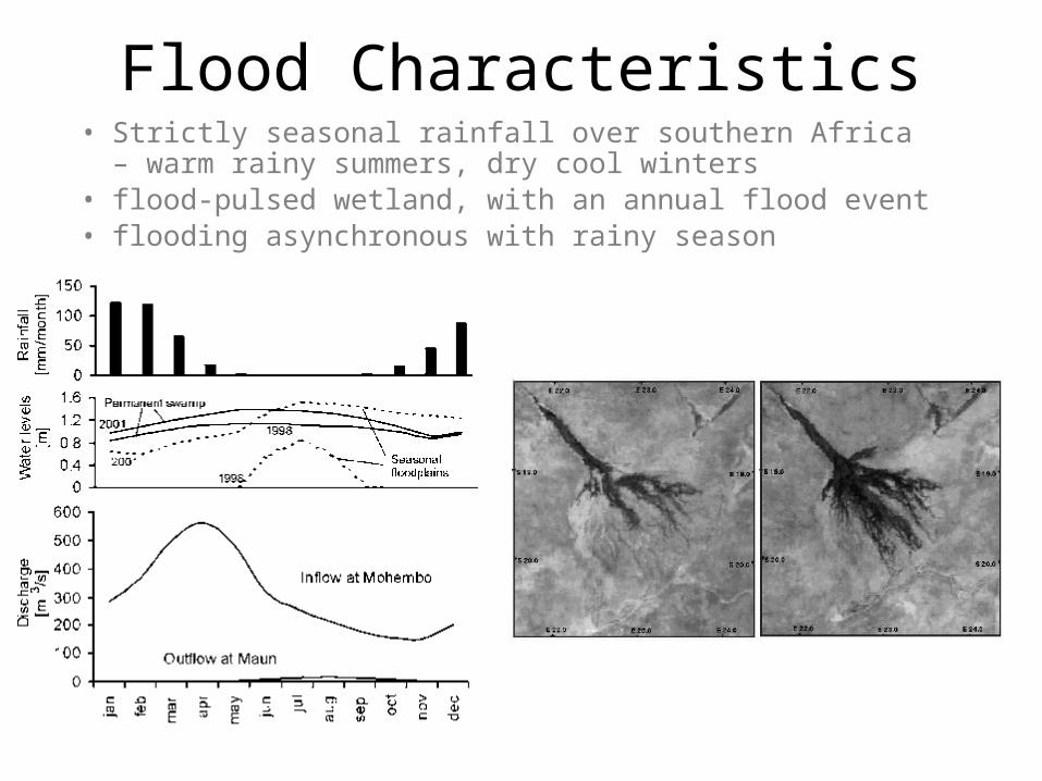
Flood Characteristics• Strictly seasonal rainfall over southern Africa – warm rainy summers,

dry cool winters• flood-pulsed wetland, with an annual flood event• flooding asynchronous with rainy season

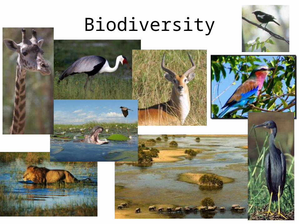
Biodiversity

High End….

To Shoot an Elephant or Lion: $75,000 for license, $50,000 for lodging, food and transportTo shoot pictures: $500-1000 per person per night

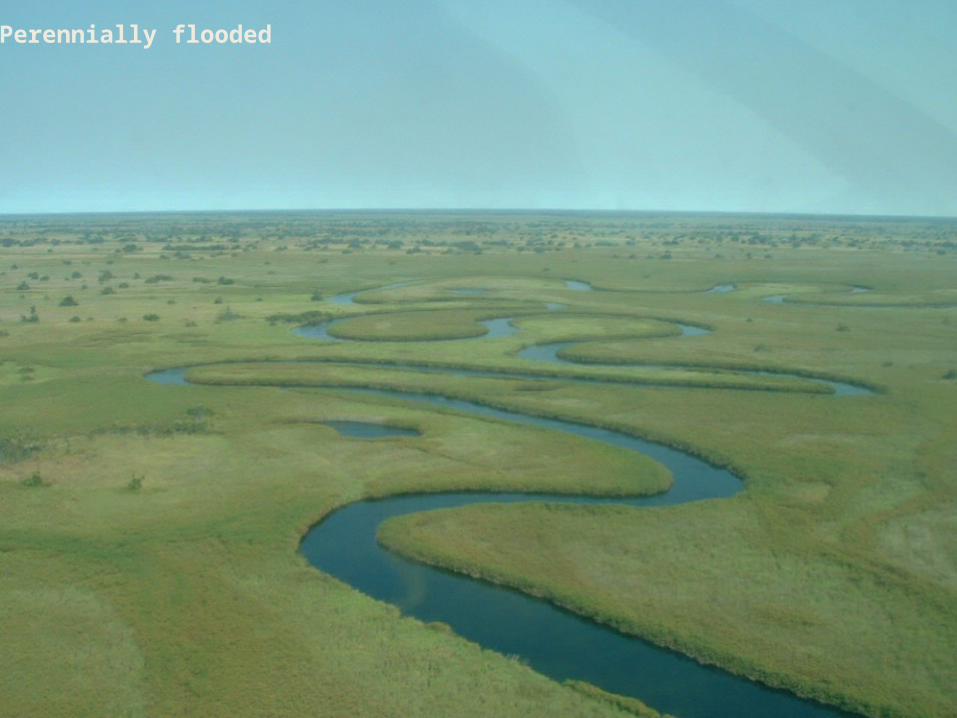
Perennially flooded

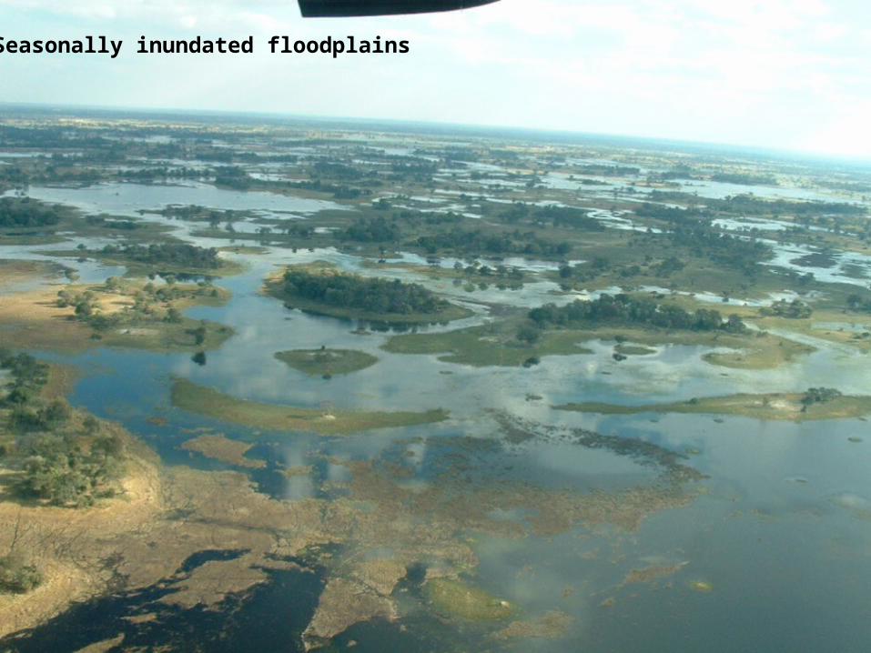
Seasonally inundated floodplains

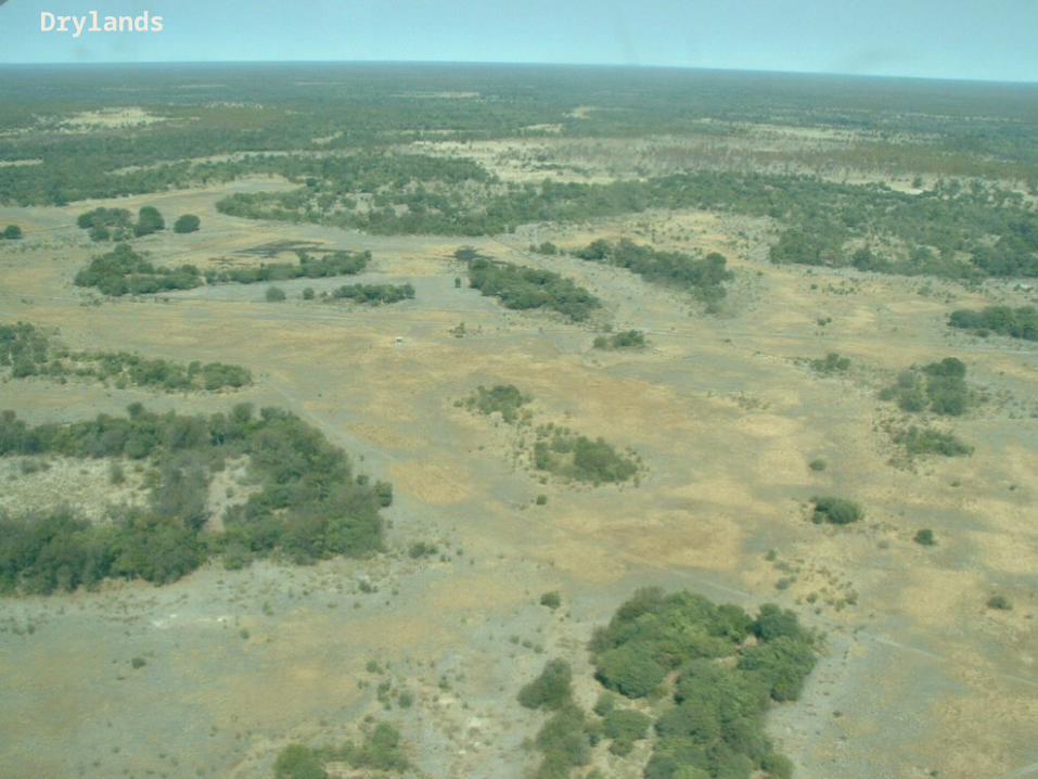
Drylands

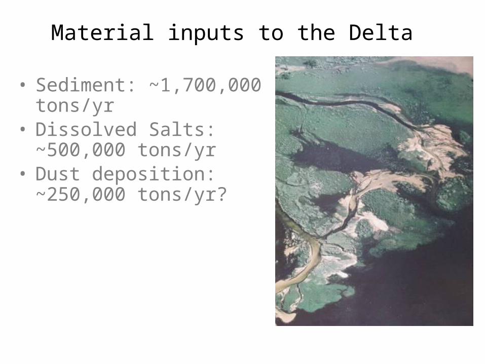
• Sediment: ~1,700,000 tons/yr• Dissolved Salts: ~500,000

tons/yr• Dust deposition: ~250,000

tons/yr?

Material inputs to the Delta

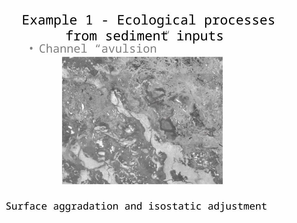
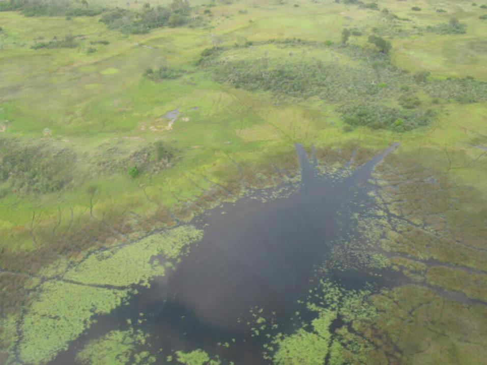
• Channel “avulsion”

Example 1 - Ecological processes from sediment inputs

Surface aggradation and isostatic adjustment

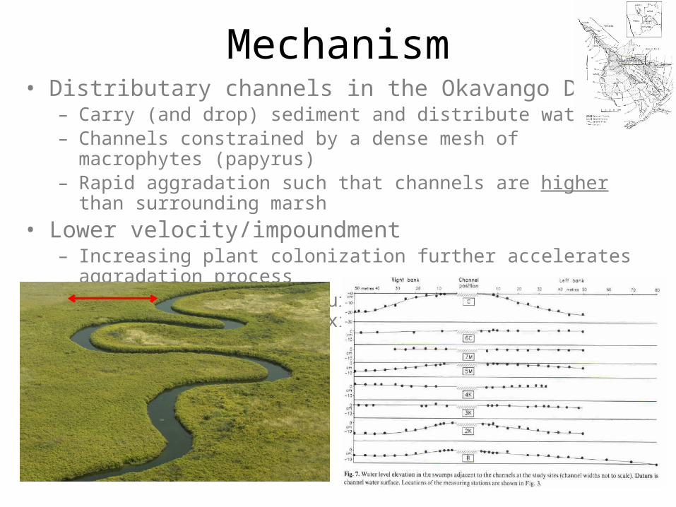
Mechanism• Distributary channels in the Okavango Delta

– Carry (and drop) sediment and distribute water– Channels constrained by a dense mesh of macrophytes (papyrus) – Rapid aggradation such that channels are higher than surrounding marsh

• Lower velocity/impoundment– Increasing plant colonization further accelerates aggradation process– Catastrophic bank failure and new channel initiation along pre-existing

hippo trails

McCarthy et al. (1992)

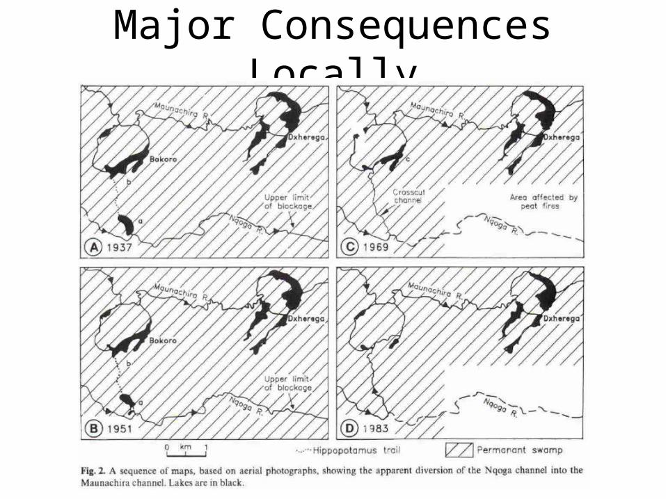
Major Consequences Locally

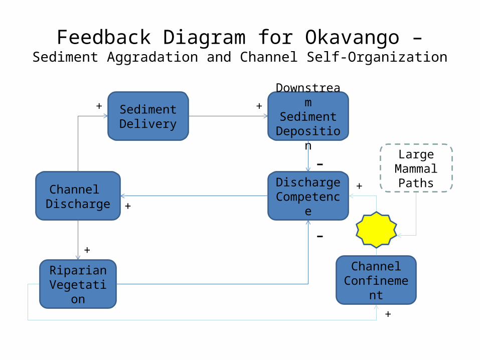
Feedback Diagram for Okavango – Sediment Aggradation and Channel Self-Organization

ChannelConfinement

Channel Discharge

-

Sediment Delivery

DownstreamSediment

Deposition

DischargeCompetence

+ +

+

+

RiparianVegetation

+-

+

LargeMammal

Paths

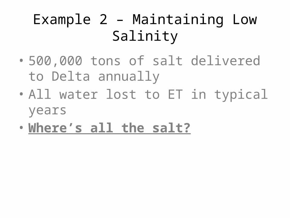
Example 2 – Maintaining Low Salinity

• 500,000 tons of salt delivered to Delta annually

• All water lost to ET in typical years• Where’s all the salt?

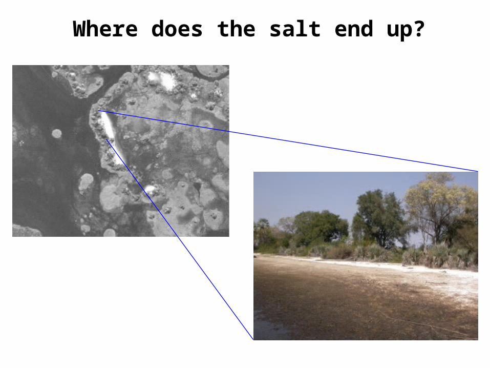
Where does the salt end up?

Island building and density fingering

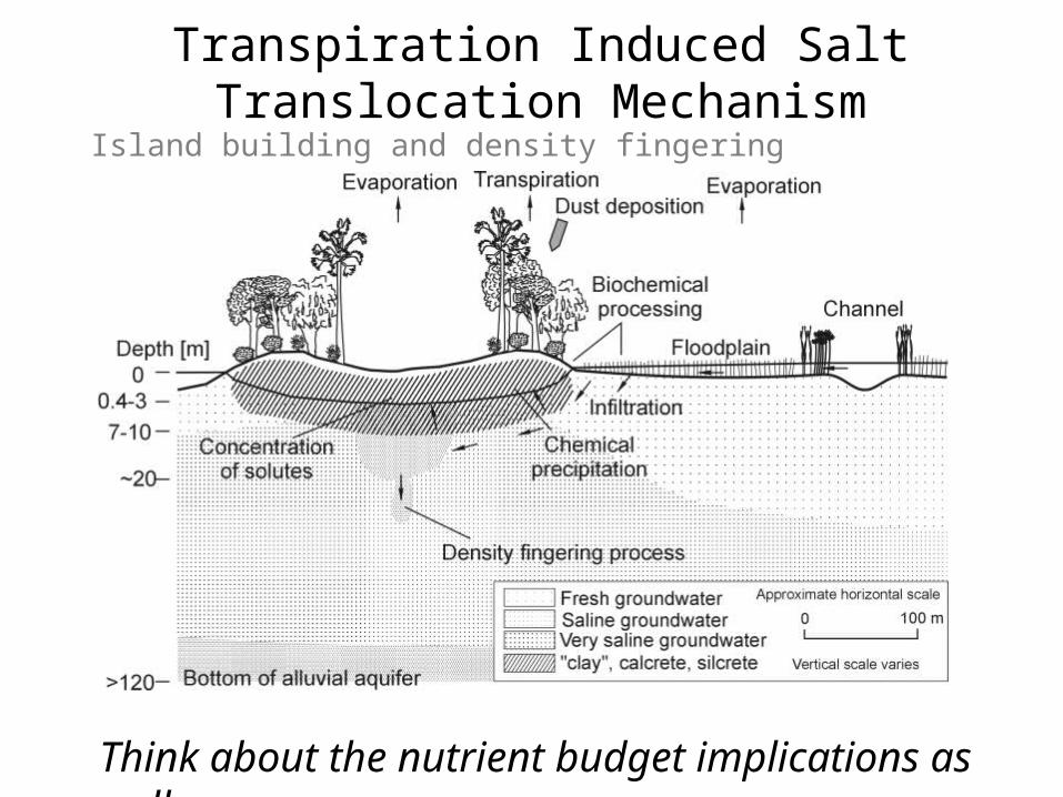
Transpiration Induced Salt Translocation Mechanism

Think about the nutrient budget implications as well

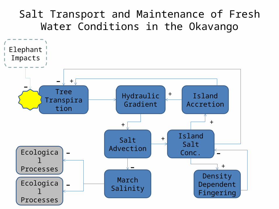
Salt Transport and Maintenance of Fresh Water Conditions in the Okavango

Island Salt Conc.

Tree Transpiration

-Salt

Advection

Density Dependent Fingering

+

+

+

+

HydraulicGradient

Elephant Impacts

-

Ecological Processes

March SalinityEcological

Processes

-

-

-

Island Accretion

+

- +

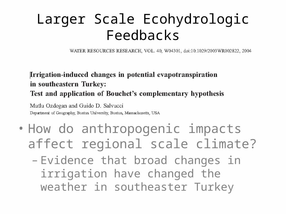
Larger Scale Ecohydrologic Feedbacks

• How do anthropogenic impacts affect regional scale climate?– Evidence that broad changes in irrigation have

changed the weather in southeaster Turkey

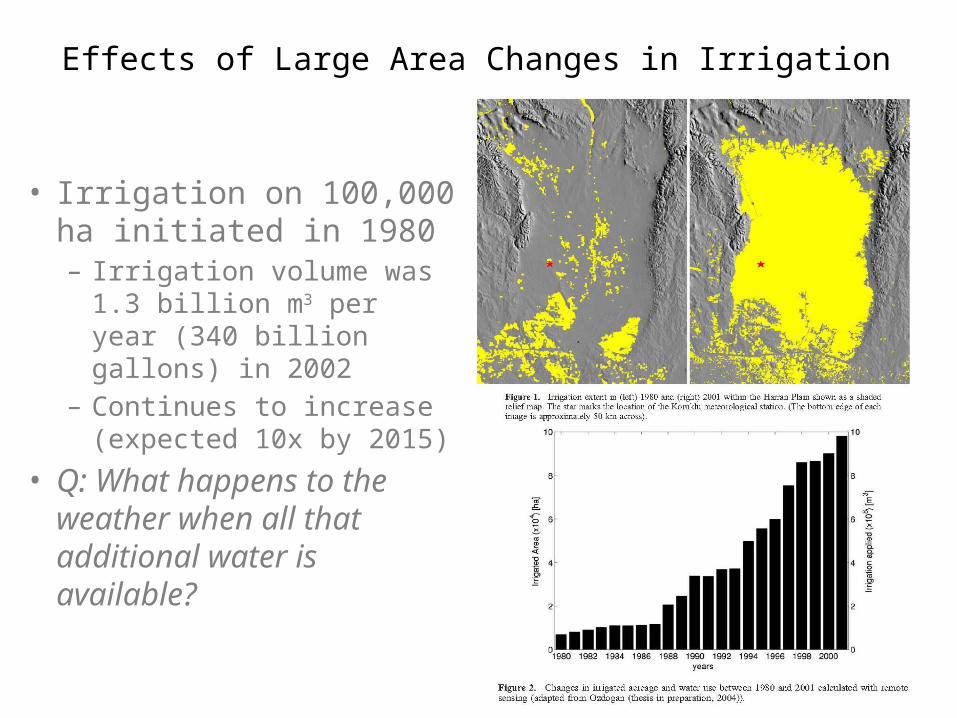
Effects of Large Area Changes in Irrigation

• Irrigation on 100,000 ha initiated in 1980– Irrigation volume was 1.3

billion m3 per year (340 billion gallons) in 2002

– Continues to increase (expected 10x by 2015)

• Q: What happens to the weather when all that additional water is available?

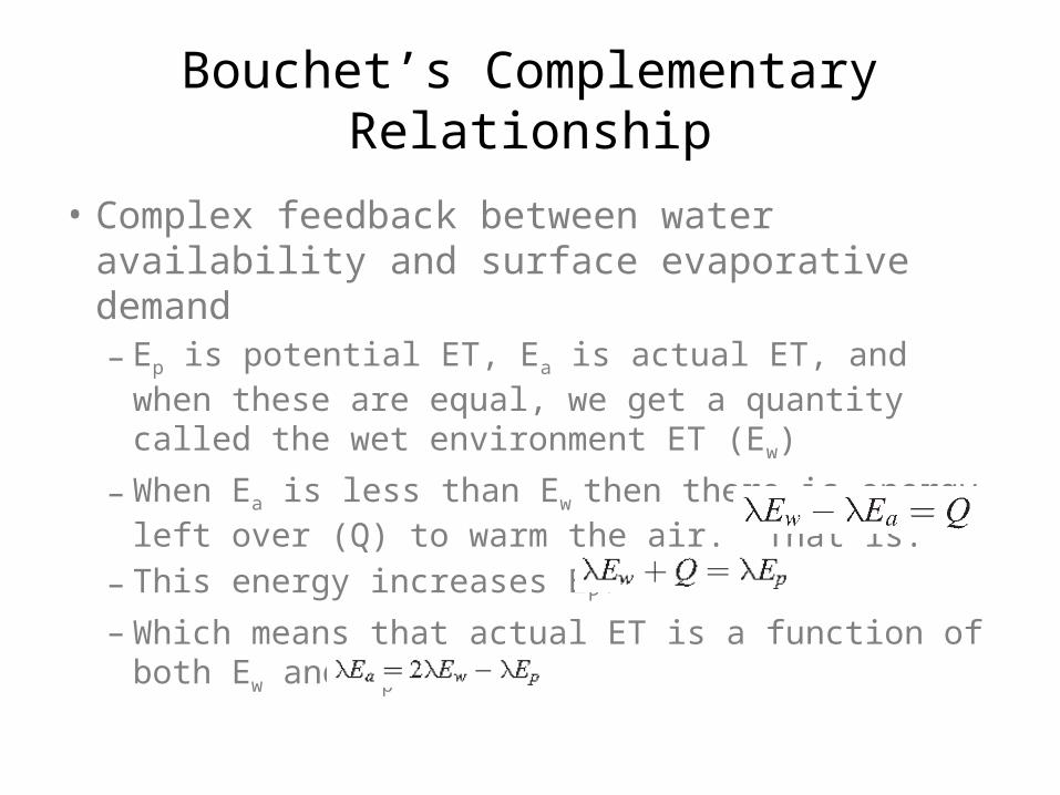
Bouchet’s Complementary Relationship

• Complex feedback between water availability and surface evaporative demand– Ep is potential ET, Ea is actual ET, and when these are

equal, we get a quantity called the wet environment ET (Ew)

– When Ea is less than Ew then there is energy left over (Q) to warm the air. That is:

– This energy increases EP:

– Which means that actual ET is a function of both Ew and Ep:

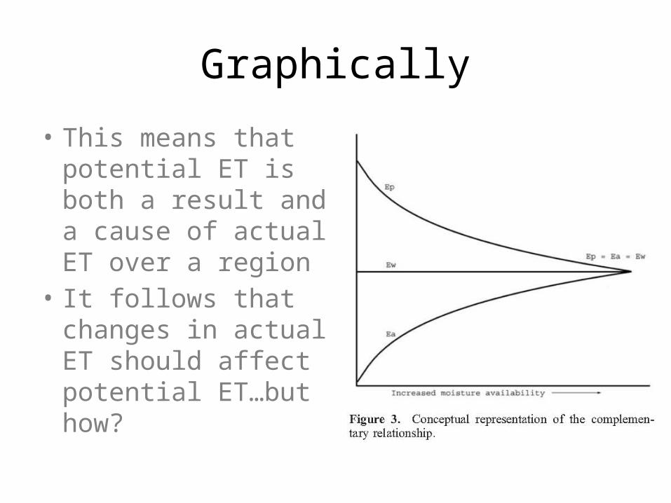
Graphically

• This means that potential ET is both a result and a cause of actual ET over a region

• It follows that changes in actual ET should affect potential ET…but how?

Results

• Potential ET declined dramatically with irrigation between 1980 and 2002– From 14 to 7 mm/d

• Causal mechanism could be changes in:– Available energy– Wind speed

(aerodynamic resistance)– Temperature or– Saturation deficit

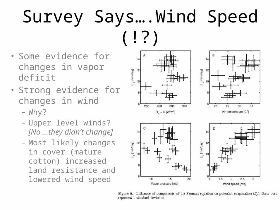
Survey Says….Wind Speed (!?)

• Some evidence for changes in vapor deficit

• Strong evidence for changes in wind– Why?– Upper level winds? [No

…they didn’t change]– Most likely changes in

cover (mature cotton) increased land resistance and lowered wind speed

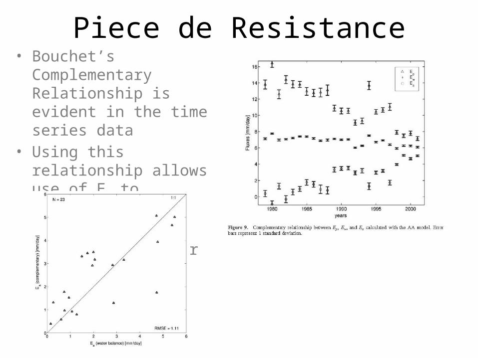
Piece de Resistance• Bouchet’s Complementary

Relationship is evident in the time series data

• Using this relationship allows use of EP to estimate Ea directly, rather than rely on water balance data

In Short

• Changes in water availability can change cover which can change the regional atmosphere.

• Or…irrigation can change the wind.

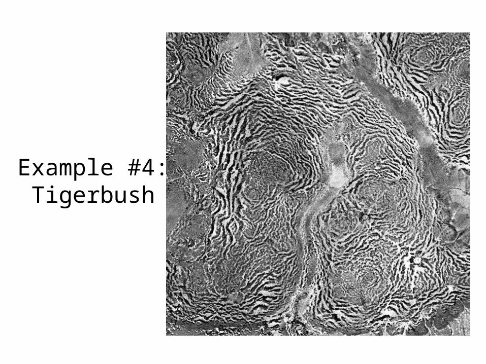
Example #4: Tigerbush

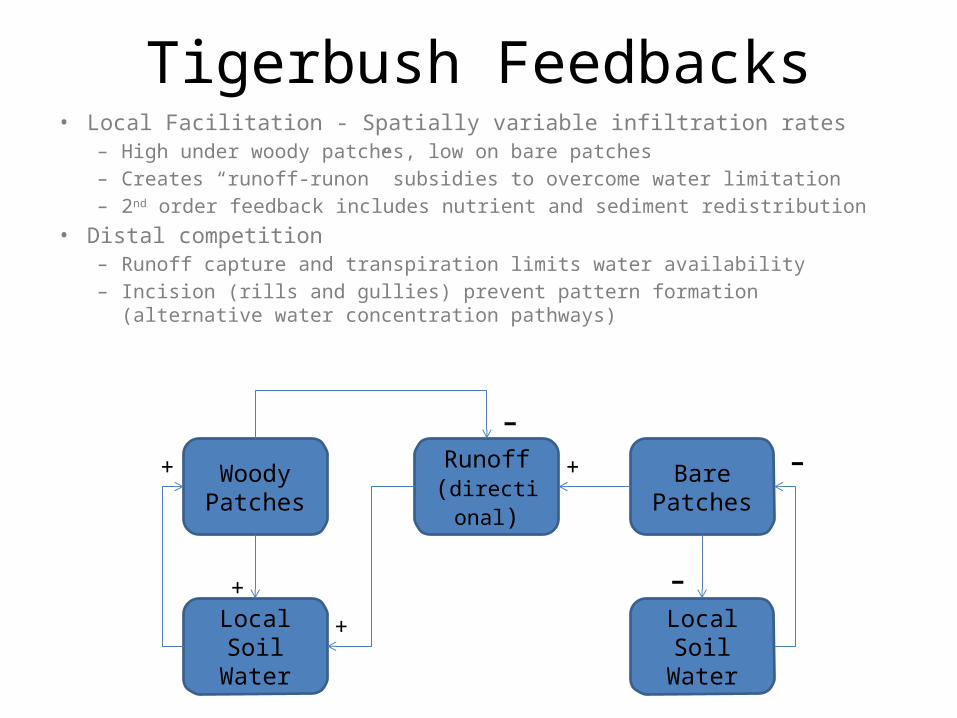
Tigerbush Feedbacks• Local Facilitation - Spatially variable infiltration rates

– High under woody patches, low on bare patches– Creates “runoff-runon” subsidies to overcome water limitation– 2nd order feedback includes nutrient and sediment redistribution

• Distal competition– Runoff capture and transpiration limits water availability– Incision (rills and gullies) prevent pattern formation (alternative water

concentration pathways)

WoodyPatches

BarePatches

LocalSoil Water

LocalSoil Water

Runoff(directional)

+

+

+

+

-

-

-

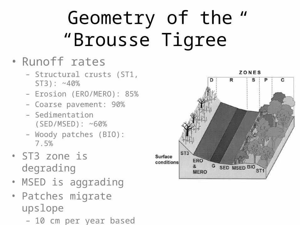
Geometry of the “Brousse Tigree”

• Runoff rates– Structural crusts (ST1, ST3): ~40%– Erosion (ERO/MERO): 85%– Coarse pavement: 90%– Sedimentation (SED/MSED): ~60%– Woody patches (BIO): 7.5%

• ST3 zone is degrading• MSED is aggrading• Patches migrate upslope

– 10 cm per year based on 137Cs data

Valentin and Herbes (1999)

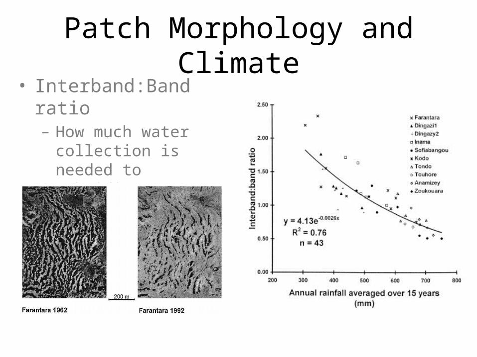
Patch Morphology and Climate• Interband:Band ratio

– How much water collection is needed to subsidize tree growth?

– Ranges from 0.5 to 2.4

Valentin and Herbes (1999)

Ra = 426 mmIBR = 1.13

Ra = 315 mmIBR = 2.30

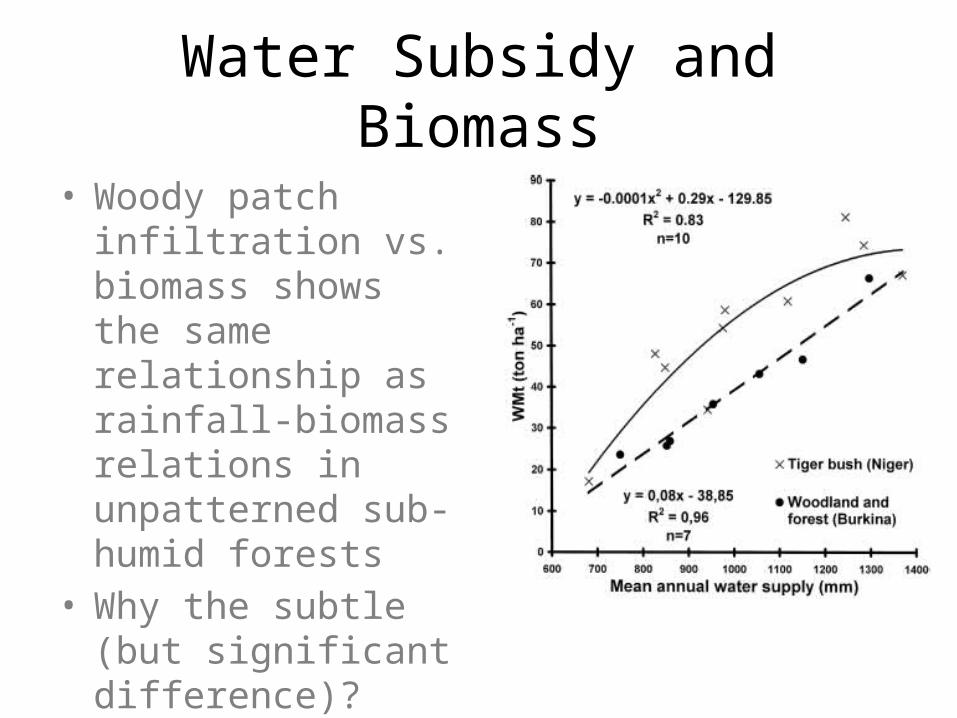
Water Subsidy and Biomass

• Woody patch infiltration vs. biomass shows the same relationship as rainfall-biomass relations in unpatterned sub-humid forests

• Why the subtle (but significant difference)?

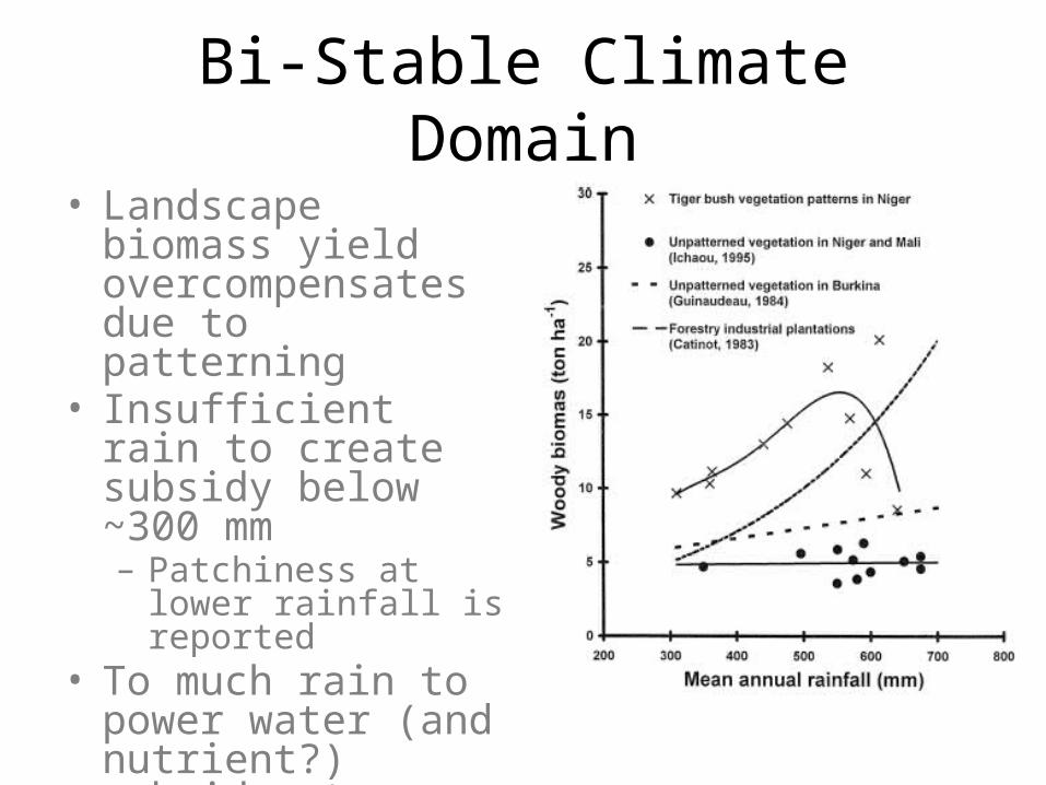
Bi-Stable Climate Domain• Landscape biomass yield

overcompensates due to patterning

• Insufficient rain to create subsidy below ~300 mm– Patchiness at lower

rainfall is reported• To much rain to power

water (and nutrient?) subsidy at ca. 650 mm– Why?

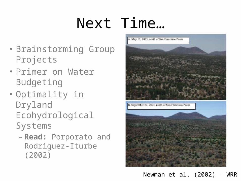
Next Time…

• Brainstorming Group Projects

• Primer on Water Budgeting

• Optimality in Dryland Ecohydrological Systems– Read: Porporato and

Rodriguez-Iturbe (2002)

Newman et al. (2002) - WRR