Ecological outbreak dynamics and the cusp catastrophe

Ecological outbreak dynamics and the cusp catastrophe

MICHAEL R. ROSE* and RUDOLF HARMSEN

Biology Department, Queen's University, Kingston, K7L 3N6, Canada

(Received 13- V-1981)

Abstract. Many ecological processes exhibit trajectories which can be suitably represented by stable equilibria or smooth limit cycles. However, a third kind of ecological process involves intermittent, abrupt, and drastic changes in densities, here termed 'outbreak dynamics', which require different modelling frameworks. One such framework, the cusp catastrophe, is used here in a modelling study of a particular outbreak insect, the forest tent caterpillar. This model is then generalized to cover a set of related ecological systems. The particular form of the model for each system depends on whether the major controlling ecological variables are externally imposed, or are in- corporated in the model equations. It is concluded that the simple cusp catastrophe is an appropriate metaphor for understanding outbreak dynamics.

1. Introduction

1.1. Ecological phenomena versus ecological models

In developing useful models of ecological systems, it is natural that the mathematical assumptions underlying each model should be both trans- parent and approrpiate to the kind of ecological dynamics represented. That is, the mathematics should be well-suited to the ecology. Since many ecological interactions appear to result in stable and enduring population densities, it is reasonable that theoretical ecology generally has concentrated on local stability conditions for unique population density equilibria (Smith, 1974; May, 1974). In addition, there are ecological interactions which give rise to sustained density oscillations, such as predator-prey dynamics, and it is appropriate that theoretical ecology should seek to characterize such dynamics in terms of smooth limit cycles (May, 1972; Gilpin, 1972). Thus, the mathematics of theoretical ecology are reasonably

* Present address: Biology Department, Dalhousie University, Halifax, B3H 4J1, Canada.

Acta Biotheoretica 30, 229-253 (1981) 0001-5342/81/0304-0229 $03. 75. (~) I QR I Mart inlJe lViih,~f£1hthli~h~,r.~ Tha Ha971e Printed in the Netherlands.

230

commensurate with some of the major phenomena of real-world ecology, as we understand it.

But there are also major exceptions. There is, for instance, a class of ecological interactions which leads to abrupt, almost explosive, changes in density, both sudden increases and swift collapses, yet multiple stable points also appear to arise. Examples of ecological situations wherein such dynamics arise are insect outbreak, disease epidemics, and species invasions of new ranges. Just as it was natural for theoretical ecology to determine conditions for unique stable equilibria and smooth limit cycles.when modelling the first two kinds of ecological dynamics, so it may be argued that it is not appropriate to begin with such an approach when modelling this third kind of ecological dynamics (Holling, 1973).

To simplify the discussion, we propose that this sort of ecological dynamics be called outbreak dynamics, as we believe that outbreak pest species exhibit such dynamics as clearly as any other group, and the term outbreak seems semantically appropriate. Some major features appear to be typical of such dynamics. There seem to be different rates of change in ecosystems exhibiting outbreaks, sometimes very fast and sometimes moderate. Fast outbreak dynamics, the sudden collapses and increases in density mentioned above, frequently appear to be triggered by the achieve- ment of meteorological and other pre-conditions, though not always. There appears to be some indeterminacy involved, which allows exogenous factors, such as weather, to play a major role. Often, it seems as if a population density threshold must be crossed before rapid changes can occur. But outbreak dynamics have remained poorly understood, and the underlying causes of these basic features, and, indeed, their quantitative nature, have re- tained an enigmatic quality.

In this paper, we attempt to illustrate how an analysis in terms of an elementary cusp catastrophe can account for these features of outbreak dynamics in a simple and intuitively clear way, and so is well-suited to modelling such dynamics. This is done by developing a cusp catastrophe model for a particular case, using empirical evidence fairly directly, and then generalizing this model to a class of related outbreak situations. In doing so, we try to show how one might go about developing models for other classes of outbreak dynamics, using the elementary catastrophes as basic tools, and what the problems are in analyzing such models. Elements of this approach have appeared before (Harmsen, Rose & Woodhouse, 1976; Jones, 1977; May, 1977; Rose & Harmsen, 1978), but its special importance for outbreak dynamics has not been made sufficiently clear. This is what we seek to do here.

1.2. The dynamics o f insect outbreaks

Insect outbreaks are among the cases where ecological outbreak dynamics are clear and dramatic. Thus their study seems to promise potential break-

231

throughs in our understanding of outbreaks, particularly in the case of issues such as endogenous versus exogenous population regulation, where insect species' density fluctuations have been important test cases (Andre- wartha & Birch, 1954). It is not surprising, therefore, that insect outbreaks have often been studied by ecologists. The studies of Baird (1917), Chap- man (1939), Utida (1958), Neilson & Morris (1964), as well as Baltens- weiler (1970) are examples of the sustained attention insect outbreaks, in particular and in general, have received.

Yet the factors which determine these outbreaks have typically remained obscure. This is in spite of the great amount of data which has been collected from some outbreak insect populations, such as those of the spruce budworm (Morris, 1963). Still, some workers have claimed to account for oscillatory outbreak dynamics in certain species, for example Wellington (1957, 1960, 1964) who studied the western tent caterpillar, and their conclusions have achieved wide currency. But the ecology of outbreak species which have been long-standing objects of study often remains a matter of controversy, particularly with regard to the factors triggering and terminat- ing outbreaks. The forest tent caterpillar, discussed below, is but one example of this. Irrespective of the success some authors have achieved with particular species, there can be no disputing the lack of general insights into insect outbreaks.

The widespread failure to illuminate the basic causality of insect outbreaks might be attributed to a lack of understanding of the idiosyncratic features of such outbreaks. As discussed by Schwerdtfeger (Varley, 1949) and Holling (1973), among others, outbreak insect dynamics have a number of characteristic features, though no one species necessarily exhibits all of them. A crude listing might be as follows. (1) Rapid onset of high densities, with further population growth proceeding to very high densities. (2) A characteristic, seemingly 'stable', ecology at high densities, with a particular pattern of disease incidence, parasitism, etc. (3) Abrupt collapse of high densities, followed by quite low densities. (4) A characteristic, seemingly 'stable', ecology at low to moderate densities, markedly different from that at high to very high densities. (5) Weather playing some unclear role in the transitions between high and low densities. (6) The semblance of threshold species densities for both onset and collapse of oubreak, irrespective of weather.

We suggest that the avenue to better overall understanding of insect outbreak would be the development of models which are suited to the respresentation of such dynamics. The particular interactions between outbreak insect and their parasites, diseases, habitats, etc., have often proved susceptible to detailed empirical investigation, and, in any event, vary widely from species to species. So a suitable model for the present purposes might effectively concentrate on the aggregate effects of subsidiary ecosystem components without representing the detailed processes within each component. Let us now illustrate this approach.

232

2. The outbreak dynamics of the forest tent caterpillar

2.1. FieM ecology

The forest tent caterpillar Malacosoma disstria Hfibn (Lepidoptera: Lasio- campidae) provides a characteristic example of outbreak dynamics. This species has been the subject of considerable investigation since the turn of the century (e.g., Evans, 1905; Tothill, 1919; Hodson, 1941; Sippel, 1957; Ives, 1973; Witter, Mattson, & Kulman, 1975). Though its complex ecology has resisted complete analysis, certain aspects of its overall dynamics are quite clear. Very high peak densities occur intermittently. While these density peaks are not periodic sensu strictu, as was once thought, they do conform to a locally consistent pattern of isolated pockets of density build- ups, swiftly spreading high densities, a density peak, a density crash, and a period of very low densities, with the species rare (Hodson, 1941 ; Sippel, 1957 and 1962). During the caterpillar's density peaks, some parasites increase to high densities and viral disease is widespread (Sippel, 1957). But, in spite of the abundance of data collected from natural populations of this species, the underlying causes of its violent density fluctuations remain controversial (Rose, 1976).

Recent experiments have revealed a crucial, hitherto unknown, facet of forest tent caterpillar ecology. It appears that the forest inhabited by the caterpillar, at least in southeastern Ontario, is made up of two distinct habitats: (1) large, connected, and dry upland areas, and (2) isolated pockets of wet lowland. This second type of habitat appears to function as a refuge, with statistically significant reductions in mortality compared with the surrounding uplands (Rose, 1976; Harmsen & Rose, 1981). Moreover, field collections between outbreaks have discovered the caterpillar only in such lowlands, suggesting that the caterpillar (i) is eliminated from the dry uplands at low densities, (ii) seeks out such wet lowlands preferentially, or (iii) both. Yet high density populations spread throughout the forest, suggesting that there is a density threshold beyond which population density increases occur in the uplands. In the sequel, an attempt is made to explain these seemingly anomalous phenomena.

The data obtained both from experiments and field observations strongly suggest that populations of the forest tent caterpillar exhibit more than one stable population density equilibrium when subject to certain levels of parasitism and disease as well as certain patterns of habitat utilization. In particular, there seem to be (i) equilibria at fairly low densities which occur in conjunction with (ii) equilibria at quite high densities. In the first case, the population is established only in the lowlands. That part of the population which is in the uplands has a negative rate of population growth. Effectively, it is eliminated. In the second, the population is established in both upland and lowland, with both parts of the population apparently at high equilibrium densities. In between the high and low total population

233

density equilibria, there appears to be a density threshold, below which the population is forced back to the lowlands and above which it becomes established throughout the forest.

The evidence is as follows. Field data provide evidence indicating that outbreak populations, which are spread out over both upland and lowland, do achieve stable equilibria at outbreak densities (Witter et al., 1975), though the biological parameters on which the equilibria depend change during outbreaks, so as to undermine the existence of such equilibria. All reports on collapsing outbreaks (e.g., Sippel, 1957; Witter et al., 1975) do not indicate any density stabilization at intermediate densities. Sampling of some low density Ontario forest tent caterpillar populations from year to year reveals no tendency to extinction or outbreak (our unpublished data). None of this evidence is direct or unequivocal, but an overall picture is be- ginning to emerge.

2.2. Development o f a cusp model

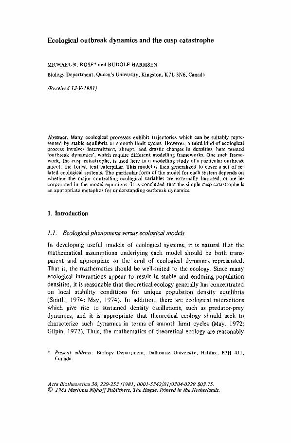
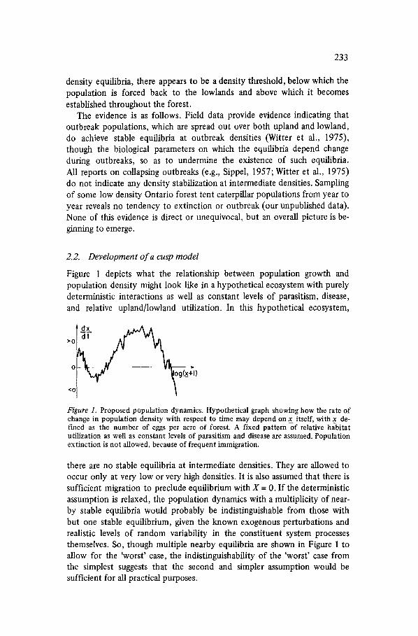
Figure 1 depicts what the relationship between population growth and population density might look like in a hypothetical ecosystem with purely deterministic interactions as well as constant levels of parasitism, disease, and relative upland/lowland utilization. In this hypothetical ecosystem,

d! >0

\ "'togI _ l

Figure 1. Proposed population dynamics. Hypothetical graph showing how the rate of change in population density with respect to time may depend on x_ itself, with x defined as the number of eggs per acre of forest. A fixed pattern of relative habitat utilization as well as constant levels of parasitism and disease are assumed. Population extinction is not allowed, because of frequent immigration.

there are no stable equilibria at intermediate densities. They are allowed to occur only at very low or very high densities. It is also assumed that there is sufficient migration to preclude equilibrium with X = 0. If the deterministic assumption is relaxed, the population dynamics with a multiplicity of nearby stable equilibria would probably be indistinguishable from those with but one stable equilibrium, given the known exogenous perturbations and realistic levels of random variability in the constituent system processes themselves. So, though multiple nearby equilibria are shown in Figure 1 to allow for the 'worst' case, the indistinguishability of the 'worst' case from the simplest suggests that the second and simpler assumption would be sufficient for all practical purposes.

234

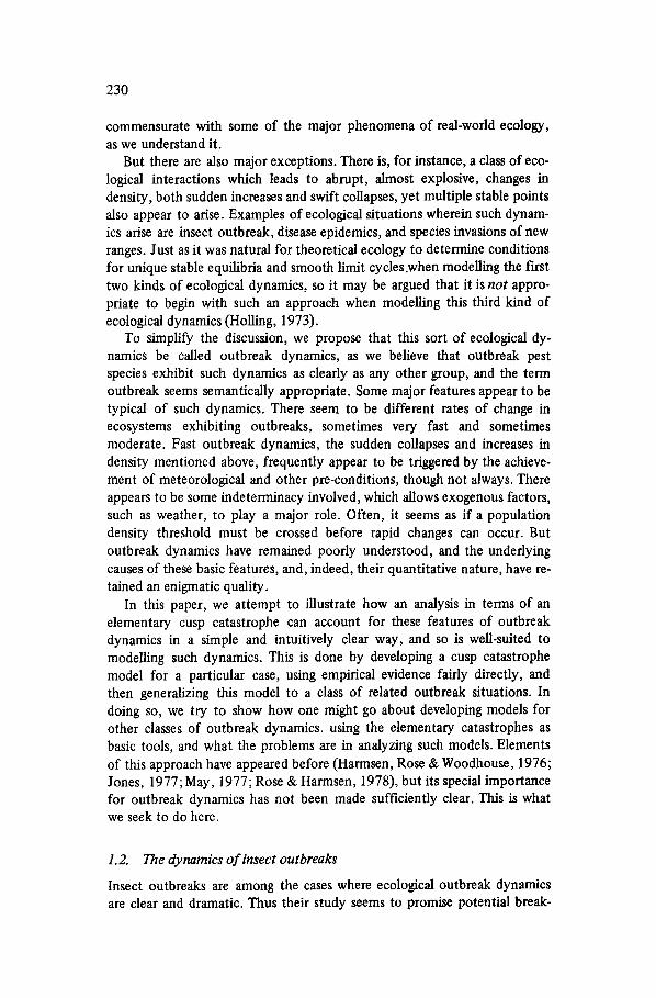
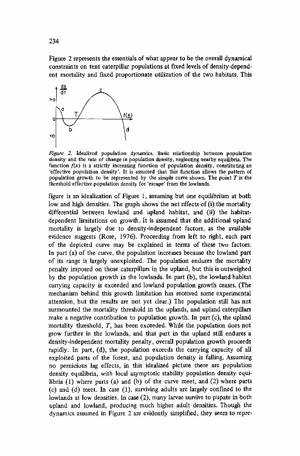
Figure 2 represents the essentials of what appear to be the overall dynamical constraints on tent caterpillar populations at fixed levels of density-dependent mortality and fixed proportionate utilization of the two habitats. This

>0

0

<0

dx_

b / d

Figure 2. Idealized population dynamics. Basic relationship between population density and the rate of change in population density, neglecting nearby equilibria. The function f(x_) is a strictly increasing function of population density, constituting an 'effective population density'. It is assumed that this function allows the pattern of population growth to be represented by the simple curve shown. The point T is the threshold effective population density for 'escape' from the lowlands.

figure is an idealization of Figure 1, assuming but one equilibrium at both low and high densities. The graph shows the net effects of (i) the mortality differential between lowland and upland habitat, and (ii) the habitat- dependent limitations on growth. It is assumed that the additional upland mortality is largely due to density-independent factors, as the available evidence suggests (Rose, 1976). Proceeding from left to right, each part of the depicted curve may be explained in terms of these two factors. In part (a) of the curve, the population increases because the lowland part of its range is largely unexploited. The population endures the mortality penalty imposed on those caterpillars in the upland, but this is outweighed by the population growth in the lowlands. In part (b), the lowland habitat carrying capacity is exceeded and lowland population growth ceases. (The mechanism behind this growth limitation has received some experimental attention, but the results are not yet dear.) The population still has not surmounted the mortality threshold in the uplands, and upland caterpillars make a negative contribution to population growth. In part (c), the upland mortality threshold, T, has been exceeded. While the population does not grow further in the lowlands, and that part in the upland still endures a density-independent mortality penalty, overall population growth proceeds rapidly. In part, (d), the population exceeds the carrying capacity of all exploited parts of the forest, and population density is falling. Assuming no pernicious lag effects, in this idealized picture there are population density equilibria, with local asymptotic stability population density equilibria (1) where parts (a) and (b) of the curve meet, and (2) where parts (c) and (d) meet. In case (1), surviving adults are largely confined to the lowlands at low densities. In case (2), many larvae survive to pupate in both upland and lowland, producing much higher adult densities. Though the dynamics assumed in Figure 2 are evidently simplified, they seem to repre-

235

sent some aspects pf the known ecology quite well, though we still do not know all the particular mechanisms determining the depicted relationship. It also remains to explain how threshold densities are exceeded, how outbreaks arise, and how they finally collapse.

In order to do this, Figure 2 must somehow be generalized to model the other salient features of forest tent caterpillar outbreak dynamics. These follow. Firstly, well-established lowland populations have not been found to disperse to the uplands in any detectable quantities between outbreaks. Thus the pattern of dispersion must change during the outbreak cycle, with the population most widely dispersing during outbreak and remaining entirely within the lowlands between outbreaks. Secondly, it is well-known that parasitism and disease, though not predation or interspecific competition, change radically during the outbreak cycle (Hodson, 1941; Sippel, 1957). Accordingly, transformations in the dynamics of Figure 2 with changes in habitat utilization and biotic regulator densities must be in- vestigated.

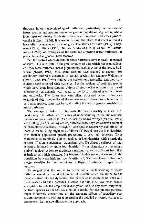
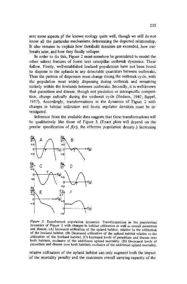
Inference from the available data suggests that these transformations will be qualitatively like those of Figure 3. (Exact plots will depend on the precise specification of f(x), the effective population density.) Increasing

dx d

ml / / "°1 \

\ c

dx ~J/ \ <o~ ~ \f(~)

Figure 3. Transformed population dynamics. Transformations in the populations dynamics of Figure 2 with changes in habitat utilization as well as overall parasitism and disease. (A) Increased utilization of the upland habitat, relative to the utilization of the lowland habitat. (B) Decreased utilization of the upland habitat relative to the utilization of the lowland habitat. (C) Increased levels of parasitism and disease over both habitats, exclusive of the additional upland mortality. (D) Decreased levels of parasitism and disease over both habitats, exclusive of the additional upland mortality.

relative utilization of the upland habitat can only augment both the impact of the mortality penalty and the maximum overall carrying capacity of the

236

utilized part of the forest, increasing the 'zig-zag' of the curve, as shown in part (A) of Figure 3; that is, increasing the distance between the mortality threshold and both the upper and lower population equilibria. With decreasing utilization of upland habitat, both the upland mortality penalty and the net carrying capacity should fall, reducing the curve's 'zig-zag', as in part (B); that is, decreasing the distance between equilibria.

Increases in parasitism and disease over the entire population should always decrease the magnitude of stable population density equilibria. But the density threshold for establishment in the uplands should increase, because increased levels of mortality can be expected to augment the impact of the additional mortality differential. These effects can be crudely represented by a vertical drop of the graph, as shown in part (C) of Figure 3. And conversely, reductions in parasitism and disease should have effects like those shown in part (D). There is little direct evidence for the indicated transformations to the population dynamics, but the proposed transformations are compatible with the available evidence.

Several limiting cases can be seen to arise. For instance, if the population is restricted entirely to the lowlands, there will be just one population density equilibrium as the 'zig-zag', parts (b) and (c) of Figure 2, should disappear altogether since they depend on the mortality penalty imposed on the upland part of the population. If parasitism and disease become very high, the population density may have only a single equilibrium level, that at low densities, as in part (E) of Figure 3. Or if parasitism and disease drop sufficiently, the mortality penalty in the uplands may not prevent population density increases in the upland at any density, eliminating the lower equilibrium, as in part (F) of Figure 3. In terms of the known changes during each outbreak, this pattern of transformation offers an explanatory metaphor for quick outbreak collapse, low between-outbreak densities, and SO o n .

But such a group of crude graphs is really just an informal sort of model. For such modelling purposes, it would be preferable to have a more explicitly unified formulation of the population dynamics, rather than a large set of graphs knitted together by a fabric of verbal argument. In fact, all the dynamical regimes which have been discussed so far can be represented by a simple cubic equation with two parameters. Re-define x such that x plus some strictly positive constant, C1, is equal to the effective total population density, the f(x) of the above figures. This re-definition could give x as a logarithm of population density, for example. In any case, note that x has now changed. Let -a be equal to the proportion of upland trees inhabited divided by the proportion of lowland trees inhabited, assuming that there is a minimum number of lowland trees always inhabited, in a single finite forest. Let b_ plus some strictly positive constant, C2, be equal to the net effective density, per caterpillar, of the parasites and diseases, weighted according to the parasite species' host specificity and the disease lethality, which affect the whole population. Using these definitions, the curves

237

discussed above have the same equilibria and equilibria transformations, with changes in dispersion, parasitism, or disease, as the following ordinary

differential equation,

dx - (x 3 + a x + b ) (1)

dt

All the crucial features of the dynamics discussed above develop naturally from equation (1) with equilibria arising and disappearing in the same fashion. Moreover, (1) is thesimplest polynomial form with the desired three real roots when a is strictly negative. (In terms of Thorn's (1969) catastrophe theory, the fight-hand side of (1) is the simple cusp catastrophe, in canonical form.) Since the present 'model ' is already highly idealized, it seems reasonable to adopt the simplest mathematical representation when re-casting it in more explicit terms.

The simple cusp arises from the general equation for a single variable dynamical system subject to two parameters:

dx • e fit = ~ = - f ( x , a_,b_) (2)

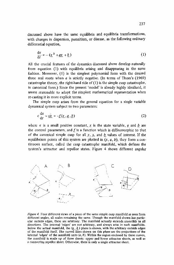
where e is a small positive constant, x is the state variable, a and b_ are the control parameters, and f_is a function which is diffeomorphic to that of the canonical simple cusp for all x, a, and b_ values of interest. If the equilibrium points of this system are plotted in (.X_, a~ b), they form a con- tinuous surface, called the cusp catastrophe manifold, which defines the system's attractor and repellor states. Figure 4 shows different angular

~ ,IL A

~ x

r 8 / , ," ¢ -

Figure 4. Four different views of a piece of the same simple cusp manifold as seen from different angles, all scales remaining the same. Though the manifold shown has particular outside edges, these are arbitrary. The manifold actually extends smoothly in all directions. The internal 'edges' are not arbitrary, and always arise in such manifolds. Below the actual manifold, the (a, b ) plane is shown, with the arbitrary outside edges of the manifold itself. The curved lines shown on this plane are the projections of the internal 'edges' of the manifold onto (a, b). Within the region enclosed by these curves, the manifold is made up of three sheets: upper and lower attractor sheets, as well as a connecting repellor sheet. Otherwise, there is only a single attractor sheet.

238

views of such a simple cusp manifold. The associated dynamical system state

effectively tends to remain on the upper and lower folds of the manifold, jumping between them at internal edges. Zeeman (1972) describes the behaviour of such systems at length.

For the forest tent caterpillar, however, a_ a n d b are not fLxed parameters,

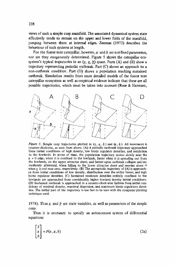
nor are they exogenously determined. Figure 5 shows the caterpillar ecosystem's typical trajectories in an ~ , a, b_) space. Parts (A) and (B) show a

trajectory representing periodic outbreak. Part (C) shows an approach to a non-outbreak condition. Part (D) shows a population reaching sustained

outbreak. Simulation results from more detailed models of the forest tent

caterpillar ecosystem as well as empirical evidence indicate that these are all

possible trajectories, which must be taken into account (Rose & Harmsen,

A

xl i

Figure 5. Simple cusp trajectories plotted in (x, a, b ) and (a, b ). All movement is counter-clockwise, as seen from above. (A) A periodic outbreak trajectory approached from initial conditions of high density, low biotic regulator densities, and restriction to the lowlands. In terms of time, the population trajectory moves slowly near the a = 0 edge, when it is confined to the lowlands, faster when it is spreading out from t-he lowlands, on the upper attractor sheet, and fastest upon outbreak collapse and im- mediately afterward, when falling to the lower attractor sheet and movinz alon~ it when a is not near zero, respectively. (B) The asymptotic trajectory of (A) is approached from initial conditions of low density, distribution over the entire forest, and high biotic regulator densities. (C) Sustained moderate densities entirely confined to the lowlands are approached from considerably higher lowland density initial conditions. (D) Sustained outbreak is approached in a counter-clock-wise fashion from initial conditions of minimal density, maximal dispersion, and maximum biotic regulatory densities. The initial part of the trajectory is too fast to be seen with the computer plotting technique used.

1978). Thus a_ and b are state variables, as well as parameters of the simple cusp.

Thus it is necessary to specify an autonomous system of differential equations

i] = F(x, a, b) (2a)

239

where F is composed of functions for 5¢, a_', and b_which generate trajectories like those of Figure 5.

We suggest that system (2a) might be a sufficient model in the following form.

e~_= -L~x, a~ b~ (3a)

-a =gl (x + d l ) + g 2 (b-+d2) (3b)

~= g3 (-a,x_ + d l ) + g 4 (~- +d l )+g5 (b__ +d2) (3c)

In such systems, a and b are termed slow variables, and equations for their rates of change are called slow equations. The constants -d 1 and -d 2 are the lower bounds of x_ andb at which the forest tent caterpillar density and the parasitoid and viral densities, respectively, are each zero. The function gl is a zero or negative-valued strictly decreasing function of x_ +_d 1 which reflects the tendency for higher densities of forest tent caterpillar populations to surmount the mortality 'barrier' about the lowlands (Rose, 1976) and spread out over the uplands, thereby decreasing a. The function g2 is a positive-valued, or zero, strictly increasing function of (b2 + d2) which reflects the tendency of forest tent caterpillar populations to remain confined to the lowlands, when suffering heavier mortality from parasitism or viral disease, due to the increased impact of the upland-lowland mortality differential when overall mortality is higher. Similarly, functions g3 and g4, both strictly increasing and zero or positive-valued, represent the de- pendence of viral disease on host contiguity and density together, and the net numerical response of the parasitoid species, respectively. Finally, g5 is a strictly decreasing, zero or negative-valued, function representing the stabilizing feedback component in the determination of parasitoid and viral densities, like the second-order term of the logistic.

2.3. Model analysis

If system (3) is indeed sufficient, it should be possible to propose specific gi which produce the system behaviour which the detailed simulation studies indicate are possible (Rose & Harmsen, 1978). In Rose & Harmsen (1978) and the Appendix, specific gi and d i are chosen which do, in fact, generate trajectories corresponding to the simulation trajectories in some detail. Thus, there are equations in the form of system (3) which can effectively replace the simulations as representations of the hypothetical caterpillar ecosystem. Moreover, system (3) models are simpler, and thus easier to analyse formally and understand intuitively.

But what can be said about the dynamics of system (3) without further specification? That is, if models conforming to system (3) are indeed the most useful representations of various hypotheses for forest tent caterpillar

240

population dynamics, what are their basic features? From the general dynamics of systems with simple cusp equation (3a), (x_, a, b) will have dynamics essentially determined by (3a) when ~ , a , b ) is off the attractor sheets. When (x, a~ b ) is on the attractor sheets, the dynamics are wholly determined by the slow equations.

As the Appendix illustrates, the dynamics determined by the slow equations can be described in terms of the isocline surfaces on which (3b) and (3c) are each zero. If there are isocline-isocline intersections which also intersect the simple cusp manifold, there will be system equilibria, which may or may not be stable. Independently of whether the system equilibria are stable or unstable, there may also be periodic attractor trajectories about them. If there are neither periodic attractors nor stable equilibria, the system may asymptotically tend to one of the five outer edges of the attractor sheets (see the Appendix).

If both the isoclines are similar to single fiat or winding planes in the (x~ a,_b) bounds of interest, then the dynamics of system (3) may be roughly characterized. If the isocline for (3b) is entirely to the left of the isocline for (3c), with (x_, _a,b) axes are in Figure 5, then the system goes to a stationary point at the lower bound for a_. Under these conditions, the model represents sustained outbreak or evenly distributed extremely low densities, depending on the fold the asymptotic state is located upon, due to the weak effect of biotic mortality on the population's tendency to spread from the lowlands. (See the Appendix.) If the (3b) isocline is entirely to the right of the (3c) isocline, the system goes to a unique stationary point at the _a = 0 boundary. This represents moderate density populations con- freed to the lowlands by heavy mortality preventing them from surmount- ing the mortality barrier about the lowlands. If neither of these conditions occurs, the isoclines must intersect and the model may exhibit periodic outbreak, fluctuating sustained outbreak densities, stable sustained outbreak densities, sustained absence of outbreak, etc.

The above analysis concentrates on the strictly deterministic properties of system (3). What are the dynamics of system (3) under stochastic perturbation? Depending on the size of the perturbation, otherwise stable equilibria or certain boundary stationary points may, in some models, lead to intermittent outbreak behaviour if the system state is perturbed sufficiently often. Consider the case of the system state near a globally stable equilibrium close to the minimum value for a_and the right edge of the upper attractor sheet in a model like that considered in the Appendix. If x__ was abruptly decreased, b was abruptly increased, or some combination of the two perturbations occurred, the system might pass beyond the local basin of attraction for the upper attractor sheet and fall to the lower attractor sheet. The basic counter-clockwise dynamics of the system would then push the population back into the lowlands and then allow outbreak to proceed until the stable outbreak equilibrium was attained once more. If the system were again perturbed, this process would repeat itself, producing a pattern of

241

intermittent outbreak. This, indeed, was the effect of perturbation on those simulation runs of Rose & Harmsen (1978) which exhibited sustained outbreak. Simulated weather produced the pattern of intermittent outbreak which would be predicted if it was assumed that models in the form of system (3) actually are sufficient representations of the simulated dynamics. (Note that system (3) is being compared with a model of totally different structure. The simulations are not based on system (3).) Similarly, it is easy to see how certain kinds of perturbation to x_, a, and b_ could disrupt the simple cusp trajectory of Figure 5, part (c), to produce intermittent outbreak, as in the simulations. Likewise, it is apparent that the cychcal trajectory of Figure 5, parts (a) and (b), would be obscured somewhat by perturbation, but need not be entirely eliminated. Again, this conforms to the simulation results. So we have found that models conforming to system (3) are sufficient substitutes for the forest tent caterpillar simulations in most important respects (Rose & Harmsen, 1978): asymptotic behaviour, response to perturbation, and so on.

Yet further, such system (3) behaviour allows a neat explanation of the role of weather in real-world caterpillar populations. If system (3) is even broadly representative of the relevant ecology, Ives' (1973) results, pointing to an interaction between weather and biotic factors, may be attributed to the potential for weather to elicit outbreak onset and collapse in the above fashion provided the endogenous biological variables are in a specific range of values corresponding to the regions close to the internal edges of the cusp attractor sheets. Therefore, for this particular and difficult case, there is a model which clearly elucidates the respective roles of what can be termed density-dependent and density-independent, or endogenous and exogenous regulatory factors.

Having shown that the cusp catastrophe can cope with outbreak dynamics in a particular case, it should be possible to develop more general cusp catastrophe models for outbreak dynamics. In the next section, this is done for a particular kind of outbreak dynamics by generalizing the variables used in the forest tent caterpillar model.

3. General cusp models for habitat-related outbreak

Having demonstrated the utility of the simple cusp for modelling one outbreak species, it seems reasonable to consider the possibility of using it to model other outbreak species. To this end, it is necessary to generalize the ecology, the model formulation, and the model analysis. Naturally, what follows must be still less concrete than the preceding material.

3.1. Ecology o f habitat-related outbreak

Consider populations of species which, like the forest tent caterpillar, have

242

a basic 'habitat', which may be a conventional habitat, a resource, or a host, which they always exploit. Typically, leaving aside predators, competitors etc., such populations are going to tend to a stable equilibrium population density determined by their species-specific carrying capacity in that habitat. Some species may have additional types of 'habitat' which they can exploit, perhaps subject to an additional mortality penalty. In such cases, the level of predation, competition, parasitism, or disease may always be such that there is still effectively only one stable population density, irrespective of the pattern of habitat utilization. But in some of these cases, threshold density effects may give rise to two or more stable population density equilibria with certain levels of predation, parasitism, etc., and certain patterns of habitat utilization.

Some examples may clarify the nature of the particular class of organ- isms of interest.

(a) Herbivores which generally exploit a specific plant which is optimal for their particular nutritional requirements, but may also exploit other, less suitable, plants. Such secondary habitat utilization will impose a mortality or fertility penalty. This penalty may be of such severity that, at low densities, individuals exploiting such plants may not make any positive net contribution to the population's growth, given certain levels of biotic regulation. Yet high density populations may exhibit mutual facilitation in the exploitation of the suboptimal habitat, allowing density increases to a second stable population density equilibrium.

(b) Agricultural pests which normally exploit a specific habitat in natural ecosystems adjacent to agricultural ecosystems. Exploitation of agricultural habitat will often entail the additional mortality penalty imposed by pestici- des and other crop practices. Again, the action of this additional mortality penalty, in conjunction with biotic regulators, may result in threshold densities for successful establishment in the agricultural habitat, much as was the case for the forest tent caterpillar's threshold for establishment in the upland.

(c) Some pathogens and parasites have alternative hosts which are not obligatory to the completion of their life-cycle. Some of these hosts will be optimal, while others may be less satisfactory for the successful completion of the life-cycle, perhaps preventing build-up of sufficient numbers for population maintenance in such hosts. Threshold effects may arise, with a particular, less satisfactory, host largely uninfected or subject to extensive epizootics. In the case of man, medical prophylaxis could create a similar mortality penalty, and epidemics of diseases which also infect other species might depend on such thresholds in some cases.

While not an exhautive list, these three examples roughly delimit the range of ecological situations in which, it is suggested, habitat-related factors can give rise to at least two stable population density equilibria (cf. May, 1977).

243

3.2. Basic features of simple cusp models

In such cases, simple cusp dynamics can arise in the same fashion as, it was argued, they do in the case of the forest tent caterpillar. In that event, the variables of equation (1) may be readily adapted, retaining x + d 1 as the effective population density, re-deffming a_ in terms of the appropriate habitat proportions, and modifying b + d 2 somewhat to cover the relevant biotic regulators, such as predators, parasites, etc. Model formulation and analysis then depend on the nature of the interactions determining a_ and b. Since the simple cusp constrains such models' dynamics within fairly stringent limits, the range of possibilities for such formulation and analysis can be explicitly spelled out.

There are four major possibilities for simple cusp models of outbreak dynamics. (I) The outbreak species density may make little contribution to the determination of a or b , in which case the onset and collapse of outbreak will depend upon the imposed pattern of habitat utilization and biotic regulation. This case is of little interest from a modelling standpoint, because model formulation cannot proceed further, and there is little scope for analysis without much additional information. (2) The outbreak species density and habitat utilization pattern may determine the level of biotic regulation, with species density and biotic regulation having little effect on the pattern of habitat utilization. In this case, model formulation and analysis centre on the dynamics of the (x_, b b) plane, perpendicular to the a_ axis, for the imposed values of a. (3) The outbreak species density and level of biotic regulation may largely determine the pattern of habitat utilization, but the level of biotic regulation may be exogenously imposed. The model is then concerned with the dynamics of the (x, a_) plane, for the given value of b. (4) Both habitat utilization and biotic regulation may be largely determined by x a , and b, in which case the formulation of the model requires consideration of the dynamics relating x,a_ and b over the entire (x, _a, b_) volume. Below, autonomous systems of nonlinear ordinary differential equations will be used to model cases (2)- (4), with the action of exogenous factors treated as system state perturbations.

In case (2), the simple cusp outbreak model takes the form

(ix ~ aT-=- (x~ +a-x + b )

(4) db ~ - = g (x ,a,b_)

where e is small, positive, and constant and g is a function of x , a_, and b which is small in magnitude compared to 1. Zeeman (1972) provides simple examples of case (2) and discusses their behaviour. The first equation is called the 'fast equation' and the second is the 'slow equation'. The fast

244

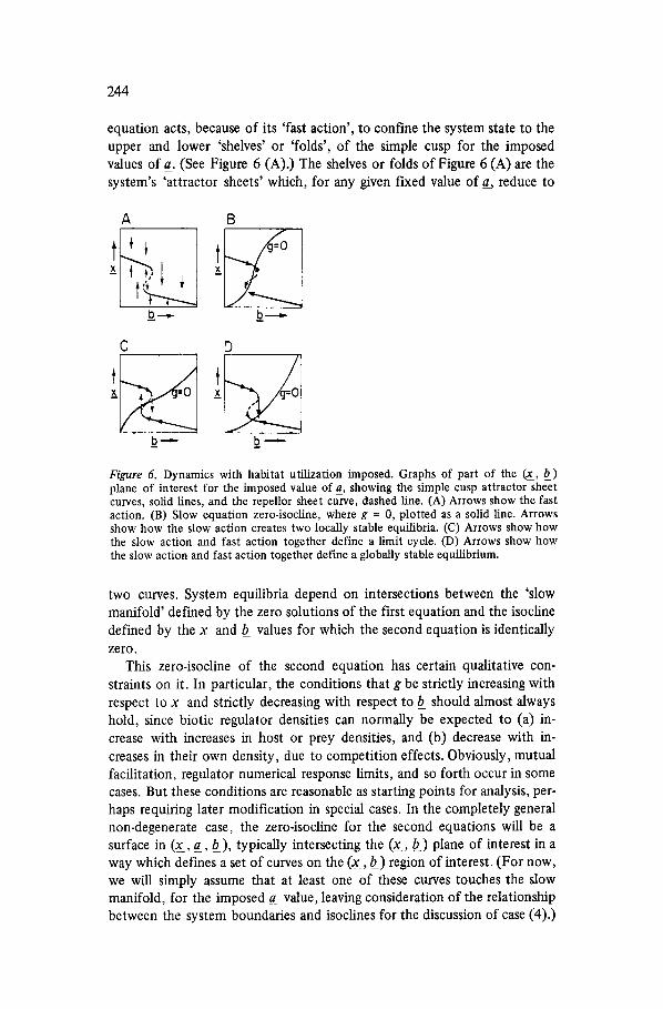
equation acts, because o f its 'fast action', to confine the system state to the upper and lower 'shelves' or 'folds', of the simple cusp for the imposed values of a_. (See Figure 6 (A).) The shelves or folds of Figure 6 (A) are the system's 'attractor sheets' which, for any given fixed value of a~ reduce to

A 8

_b ---,- _b ,,

C D

Figure 6. Dynamics with habitat utilization imposed. Graphs of part of the (x, b ) plane of interest for the imposed value of a_, showing the simple cusp attractor sheet curves, solid lines, and the repellor sheet curve, dashed line. (A) Arrows show the fast action. (B) Slow equation zero-isocline, where g = 0, plotted as a solid line. Arrows show how the slow action creates two locally stable equilibria. (C) Arrows show how the slow action and fast action together define a limit cycle. (D) Arrows show how the slow action and fast action together define a globally stable equilibrium.

two curves. System equilibria depend on intersections between the 'slow manifold' defined by the zero solutions of the first equation and the isocline defined by the x and b_ values for which the second equation is identically zero.

This zero-isocline of the second equation has certain qualitative constraints on it. In particular, the conditions that g be strictly increasing with respect to x_ and strictly decreasing with respect to b should almost always hold, since biotic regulator densities can normally be expected to (a) increase with increases in host or prey densities, and (b) decrease with increases in their own density, due to competition effects. Obviously, mutual facilitation, regulator numerical response limits, and so forth occur in some cases. But these conditions are reasonable as starting points for analysis, perhaps requiring later modification in special cases. In the completely general non-degenerate case, the zero-isocline for the second equations will be a surface in (x, a_, b_), typically intersecting the (x, b_) plane of interest in a way which defines a set of curves on the (x , b ) region of interest. (For now, we will simply assume that at least one of these curves touches the slow manifold, for the imposed _a_ value, leaving consideration of the relationship between the system boundaries and isoclines for the discussion of case (4).)

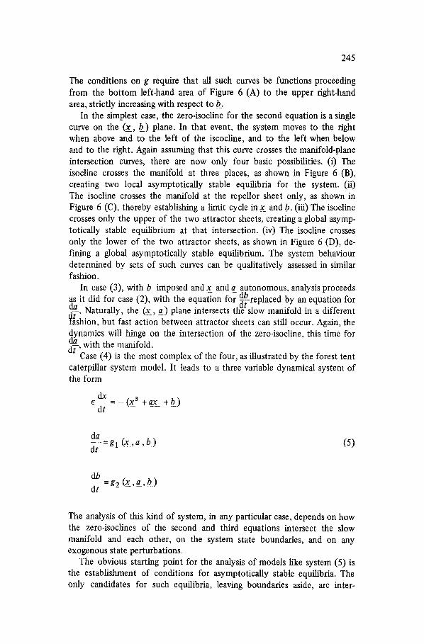
245

The conditions on g require that all such curves be functions proceeding from the bottom left-hand area of Figure 6 (A) to the upper right-hand area, strictly increasing with respect to b_.

In the simplest case, the zero-isocline for the second equation is a single curve on the (x, b) plane. In that event, the system moves to the right when above and to the left of the iscocline, and to the left when below and to the right. Again assuming that this curve crosses the manifold-plane intersection curves, there are now only four basic possibilities. (i) The isocline crosses the manifold at three places, as shown in Figure 6 (B), creating two local asymptotically stable equilibria for the system. (ii) The isocline crosses the manifold at the repellor sheet only, as shown in Figure 6 (C), thereby establishing a limit cycle in x_ and b_. (iii) The isocline crosses only the upper of the two attractor sheets, creating a global asymptotically stable equilibrium at that intersection. (iv) The isocline crosses only the lower of the two attractor sheets, as shown in Figure 6 (D), de- fining a global asymptotically stable equilibrium. The system behaviour determined by sets of such curves can be qualitatively assessed in similar fashion.

In case (3), with b imposed and x and a autonomous, analysis proceeds as it did for case (2),with the equation for db replaced by an equation for da dt ~- . Naturally, the (x_, a) plane intersects the slow manifold in a different ashion, but fast action between attractor sheets can still occur. Again, the

dynamics will hinge on the intersection of the zero-isocline, this time for da, with the manifold. at Case (4) is the most complex of the four, as illustrated by the forest tent caterpillar system model. It leads to a three variable dynamical system of the form

dx e = - ( x 3 +ax + b )

dt

da dt =gl ( x , a , b ) (5)

db dt g2 (x,a_,h.)

The analysis of this kind of system, in any particular case, depends on how the zero-isocfines of the second and third equations intersect the slow manifold and each other, on the system state boundaries, and on any exogenous state perturbations.

The obvious starting point for the analysis of models like system (5) is the establishment of conditions for asymptotically stable equilibria. The only candidates for such equilibria, leaving boundaries aside, are inter-

246

sections of the slow equation zero-isoclines with the attractor sheets, which in turn also intersect with each other. That is, points where all three system equations simultaneously equal zero. Local asymptotic stability can then be assessed by examining the eigenvalues of the Jacobian matrix of partial derivatives at the equilibrium in the usual manner. Alternatively, graphical isocline analysis can distinguish between those cases where asymptotically stable equilibria must or cannot arise, leaving a third class of equilibria requiring more explicit evaluation. In addition "to equilibria with local asymptotic stability, limit cycles may also arise. Unfortunately, the analyt- ical tools available for treating limit cycles are generally inadequate. One case where it may be possible to study limit cycles analytically occurs when it can be shown that (a) there are no stable equilibria, (b) there are no boundary stationary points, and (c) the system flow is circular. Otherwise the use of these models must rely heavily on numerical methods (cf. Rose, 1976).

For outbreak simple cusp models conforming to cases (2), (3), and (4), it is important to examine the consequences of large and infrequent perturbations to the system state, because of the known importance of factors like extreme weather (e.g., Witter et al., 1975). There are two major possibilities which should be distinguished: state perturbations of systems with multiple local asymptotically stable trajectories and state perturbations of systems with single 'precarious' locally stable asymptotic trajectories only.

In models with multiple asymptotic trajectories, two patterns of system behaviour are clearly significant, and there may be others as well. Firstly, a long-term pattern of indeterminate alternation between asymptotic trajectories with large basins of attraction may occur. The frequency of alternation will depend on the extent of each major system state perturbation. The resultant dynamics will also be influenced by the topology of the asymptotic trajectory basins and the rate of approach to these trajectories within their basins.

Secondly, in systems where some locally stable asymptotic trajectories have very small basins, system state perturbations may be so large that these asymptotic trajectories are no longer important in the long-term determination of system behaviour. An obvious example is a locally stable equilibrium on an attractor sheet surrounded by a limit cycle. If the basin of attraction about the equilibrium is sufficiently small, the system will asymptotically behave as if the limit cycle was the only local asymptotic trajectory. Other examples of the qualitative importance of perturbation with these two patterns of dynamics may be readily constructed.

The problem of models with single precarious asymptotic trajectories is more specific to catastrophe-based systems. In general, it arises when single asymptotic trajectories occur only near the edges of attractor sheets. In such situations, large perturbations may give rise to a pattern of approach to the asymptotic trajectory, perturbation past the attractor sheet edge, fast action to another attractor sheet, and then another approach to the

247

asymptotic trajectory. (This is also discussed in Section 2.3 for the particular case of the forest tent caterpillar model.)

For example, consider a simple cusp system with a global asymptotically stable equilibrium near the edge of the upper attractor sheet. Sufficient system state perturbation may give rise to dynamics which are difficult to distinguish from those of a system with a limit cycle over both attractor sheets when also subject to state perturbation. From this, it is evident that the position of asymptotic trajectories relative to the manifold edges is a very important consideration in model analysis.

4. Conclusions

We have attempted to illustrate various salient aspects of the use of elementary catastrophes in models of outbreak dynamics. Necessarily, our treatment has been both mathematically and ecologically simplistic, in order to keep the main problems of the application as clear as possible. Naturally, the mathematical details depend on the specifics of the ecological situation under investigation.

It should now be apparent that the simple cusp provides a mathematical framework which can be used to embody the idiosyncrasies of at least one kind of outbreak dynamics. Returning to the general outline of outbreak dynamics given at the outset, abrupt increases to, or collapses of, high outbreak species densities may be interpreted in terms of fast action between the attractor sheets of a catastrophe manifold. The different rates of change observed in outbreak ecosystems seem to arise from ecological dynamics which are well-characterized by fast action between catastrophe attractor sheets and slow action on these attractor sheets. 'Trigger' and 'threshold' effects can be viewed in terms of the points at which the system dynamics switch from movement on attractor sheets to movement between attractor sheets. And the important role that exogenous factors can play in such transitions can be made understandable when visualized in terms of the effects of system state perturbations in catastrophe-based systems, discussed above. In sum, it appears that catastrophe models can indeed readily represent the nature and action of the major features of outbreak dynamics.

However, there can be no denying the fact that this need not be a unique feature of catastrophe-based models. It should be possible to construct a variety of dynamical systems models which also produce trajectories like those of particular real-world outbreak ecosystems (cf. May, 1977). The potential sufficiency of other kinds of model for this purpose is indisput- able. The advantage of catastrophe-based models is their transparency and simplicity, aiding both intuition and analysis. That is, the 'catastrophic' dynamical behaviour of catastrophe models is not unique, but the straight- fora, ard way in which it arises is, relative to other modelling approaches. Since one of the central purposes of model construction is to develop

248

understanding, simplicity is no t to be disparaged. F r o m the relatively

natural way in which it was possible to develop and generalize a simple cusp

model for habitat-related outbreak dynamics, we would argue that the

e lementary catastrophes should be used as basic 'metaphors ' for outbreak

dynamics. That is, in as much as ecologists tend to think o f ecosystem

dynamics in terms o f simple mathemat ica l archetypes like stable equilibria

and l imit cycles, we would suggest that ecosystems with outbreak species

are best viewed in terms o f catastrophes. Natural ly, this is no t to assert that

such ecosystems fundamenta l ly are reducible to catastrophes. This sugges-

t ion is heurist ic, no t metaphysical .

Acknowledgements

The authors wish to acknowledge L.B. Jonker , J.M. Yee and an anonymous

reviewer for constructive crit icism of earlier drafts. This work was partly

funded by the Nat ional Science and Engineering Research Council o f

Canada through grant A3643 to RJ-I.

References

Andrewartha, H.G. & L.C. Birch (1954). The distribution and abundance of animals. - Chicago, University of Chicago Press.

Baird, A.B. (1917). An historical account of the forest tent caterpillar and of the fall webworm in North America. - Ann. Rept. Ent. Soc. Ont. 47, p. 73-84.

Baltensweiler, W. (1970). Zur Verteilung der Lepidopterenfauna auf der Laerche des Schweizerischen Mittellandes. - Mitt. Schweiz. Entomol. Ges. 42, p. 221-229.

Chapman, R.N. (1939). Insect population problems in relation to insect outbreak. - Ecol. Mon. 9, p. 261-269.

Evans, J.D. (1905). Annual address of the president. - Ann. Rep. Ent. Soc. Ont. 36, p. 49-51.

Gilpin, M.E. (1972). Enriched predator-prey systems: Theoretical stability. - Science 177, p. 902-904.

Harmsen, R. & M.R. Rose (1981). Larval survivorship in pre-outbreak populations of the forest tent caterpillar, Malacosoma disstria Htibn. (Lepidoptera: Lasiocampi- dae). - Proc. Ent. Soc. Ont. (in press).

Harmsen, R., M.R. Rose & B. Woodhouse (1976). A general mathematical model for insect outbreak. - Proc. Ent. Soc. Ont. 197, p. 11-18.

Hodson, A.C. (1941). An ecological study of the forest tent caterpillar, Malacosoma disstria Hiibn. - Minn. agric. Exp. Stn. Tech. Bull. 148, p. 1-55.

Holling, C.S. (1973). Resilience and stability of ecological systems. - Ann. Rev. Ecol. Syst. 4, p. 1-23.

Ives, W.G.H. (1973). Heat units and outbreaks of the forest tent caterpillar, Malacoso- ma disstria (Lepidoptera: Lasiocampidae). - Can. Ent. 105, p. 529-543.

Jones, D.D. (1977). Catastrophe theory applied to ecological systems. - Simulation 29, p. 1-15.

Levins, R. (1974). The qualitative analysis of partially specified systems. - Ann. N.Y. Acad. Sci. 226, p. 123-138.

May, R.M. (1972). Limit cycles in predator-prey communities. - Science 177, p. 900- 902.

249

May, R.M. (1974). Stability and complexity in model ecosystems. - Princeton, N.J., Princeton Univ. Press.

May, R.M. (1977). Thresholds and breakpoints in ecosystems with a multiplicity of stable states. - Nature, p. 471-477.

Morris, R.F. (1963). The dynamics of epidemic spruce budworm populations. - Mem. Ent. Soc. Can. 31, p. 1-332.

Neilson, M.M. & R.F. Morris (1964). The regulation of European spruce sawfly numbers in the maritime provinces of Canada from 1937 to 1963. - Can. Ent. 96, p. 773-784.

Rose, M.R. (1976). An experimental simulation, and mathematical study of an outbreak insect: the forest tent caterpillar (Lepidoptera: Lasiocampidae). Kingston, Ontario. M. Sc. Thesis, Queen's Univ.

Rose, M.R. & R. Harmsen (1978~. Using sensitivity analysis to simplify ecosystem models: a case study. Simulations31, p. 15-26.

Sippel, W.L. (1957). A study of the forest tent caterpillarMalacosoma disstria Hiibn~, and its 0arasite complex in Ontario. - Ann Arbor, Michigan, Ph.D. Thesis, Univ. of Michigan.

Sippel, W.L. (1957). A study of the forest tent caterpillar Malacosoma disstria HiJbn., and its parasite complex in Ontario. - Ann Arbor, Michigan, Ph.D. Thesis, Univ. of Michigan.

Smith, J.M. (1974). Models in ecology. Cambridge, U.K., Cambr. Univ. Press. Thorn, R. (1969). Topological models in biology. - Topology, 8, p. 313-335. Tothill, J.D. (1919). Insect outbreaks and their causes. Ann. Rep. Ent. Soc. Ont.

50, p. 31-33. Utida, S. (1958). On fluctuations in population density of the rice stem borer Chilo

suppressalis. - Ecology, 39, p. 587-599. Varley, G.C. (1949). Population changes in German forest pests. - J. Anim. Ecol.

18, p. 117-122. Wellington, W.G. (1957). Individual differences as a factor in population dynamics:

the development of a problem. - Can. J. Zool. 35, p. 293-323. Wellington, W.G. (1960). Qualitative changes in natural population during changes

in abundance. - Can. J. Zool. 38, p. 289-314. Wellington, W.G. (1964). Qualitative changes in populations in unstable environ-

ments. Can. Ent. 96, p. 436-451. Witter, J.A., W.J. Mattson, & H.M. Kulman (1975). Numerical analysis of a forest

tent caterpillar (Lepidoptera: Lasiocampidae) outbreak in northern Minnesota. - Can. Ent. 197, p. 837-854.

Zeeman, E.C. (1972). Differential equations for the heartbeat and nerve impulse. - In: Waddington, C.H. (ed.), Towards a theoretical biology, Vol. 4., Chicago, Aldine-Atherton.

250

Appendix

Consider the following special case of system (3), with x__, a , and b_ defined as before, d 1 equal to 3, d 2 equal to 3, and a_ having a minimum def'med value of -5 ; all c i positive.

= - ( x a +ax + b ) (AI.1)

d = - c 1 (x +3) 2 +c 2 ( b + 3 ) 2 (A1) (A1.2)

_b~ = -c3_a (x + 3) + c 4 (x + 3) - c s (b + 3) (A1.3)

When a_ = 0 and - c 1 (x_ + 3) 2 + c 2 (b_ + 3) 2 is greater than zero ora_ = - 5 and - c 1 (x_ + 3) 2 + c 2 (b_ + 3) 2 is less than zero, the system is defined as

=-(x? + ~ +b_)

b" = - c 3 a (x + 3 ) + c 4 ( x + 3 ) - c 5 (b_+3)

(A2.1) (A2)

(A2.2)

Two major features of the above system arise from modelling considera- tions. Firstly, the (A2) equations define the model when (x, a , b_) would otherwise cross the defined boundaries of a. This additional stipulation is not strictly accounted for in system (3). It is added in order to constrain the model system to its defined limits. These limits reflect the modelling assumption that the modelled universe is a single l~mite forest. Since this assumption is at odds with the actual situation, a realistic specification of system (3) can be expected to produce (x, a, b) trajectories which would lead to dispersion beyond the model's forest periphery if the a boundary dynamics were not re-defined. The second modelling point is that the lower a_ bound prevents jump transition from lower to upper attractor sheets when a is at its minimum because the x_ = - 3 plane cuts off the fore- ground left-hand side piece, in the orientation of Figures 7 and 8, of the lower attractor sheet. This represents the assumption that real-world low density forest tent caterpillar populations which are spread out over the entire forest cannot outbreak, irrespective of biotic regulator density. An additional consequence of this choice of a's lower bound is that populations on the upper attractor sheet near a's minimum are always also above the lower attractor sheet. This represents real-world ecology in which sustained outbreaks can always be terminated by sufficiently heavy mortality due to weather.

The dynamical possibilities for the system defined by (A1) and (A2), call it system (*), can be largely characterized in terms of the isoclines where (A1.2) and (A1.3) each equal zero. These will be referred to as the zero-isoclines. The crucial factor for the system (*) dynamics is the pattern of zero-isocline intersection with the manifold intersections for (A1.2) and

251

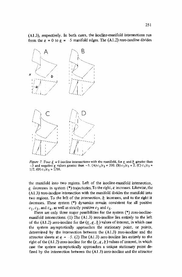
(A1.3), respectively. In both cases, the isocline-manifold intersections run from the a_ = 0 to a_ = - 5 manifold edges. The (A1.2) zero-isocline divides

i

X

B

Figure 7. Four d = 0 isocline intersections with the manifold, for x_ and b greater than -3 and negativea values greater than -5. (A) cl /c 2 = 200. (B) cl /c 2 =-2, (C) ci/c2 = 1/2, (D) cl/c2 = 1/16.

the manifold into two regions. Left of the isocline-manifold intersection, a_ decreases in system (*) trajectories.To the right, a_ increases. Likewise, the (A 1.3) zero-isocline intersection with the manifold divides the manifold into two regions. To the left of the intersection, b_ increases, and to the right it decreases. These system (*) dynamics remain consistent for all positive Cl, c3, and c4, as well as strictly positive c 2 and c 5 .

There are only three major possibilities for the system (*) zero-isocline- manifold intersections. (1) The (A1.3) zero-isocline lies entirely to the left of the (A1.2) zero-isocline for the (x , a_, b_) values of interest, in which case the system asymptotically approaches the stationary point, or points, determined by the intersection between the (AI.3) zero-isocline and the attractor sheets at a = - 5 . (2) The (A1.3) zero-isocline lies entirely to the right of the (A1.2) zero-isocline for the (x , a , b ) values of interest, in which case the system asymptotically approaches a unique stationary point defined by the intersection between the (A1.3) zero-isocline and the attractor

t

i

i

i

sheets at a_ = O. (3) The (A1.3) zero-isocline intersects the (AI .2) zero- isocline for the (x , a , b ) values of interest. In this case, system (*) has complex dynamical possibilities.

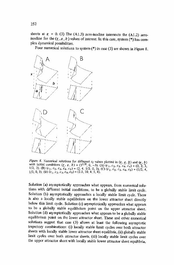
Four numerical solutions to system (*) in case (3) are shown in Figure 8.

F b '

252

[3

#

Figure 8. Numerical solutions for diffesent c i values plotted in (x, a, b) and (a, b) with initial conditions (x, a, b) = (31/3, 0, -3). (A) (cl, e2, ca. c4, c5) = (2, -2, -3, 1/2, 3), (B) (cl, c2, c3, c4, c 5) = (2, 4. 1/2, 0, 3), (C) (cl, c2, c3, c4, c5) = (1/2, 4, 1/2, 0, 3), (D) (c 1, c2, c3, c4, cs) = (2.1, 10, 4, 5, 4).

Solution (a) asymptotically approaches what appears, from numerical solutions with different initial conditions, to be a globally stable limit cycle. Solution (b) asymptotically approaches a locally stable limit cycle. There is also a locally stable equilibrium on the lower attractor sheet directly below this limit cycle. Solution (c) asymptotically approaches what appears to be a globally stable equilibrium point on the upper attractor sheet. Solution (d) asymptotically approaches what appears to be a globally stable equilibrium point on the lower attractor sheet. These and other numerical solutions suggest that case (3) allows at least the following asymptotic trajectory combinations: (i) locally stable limit cycles over both attractor sheets with locally stable lower attractor sheet equilibria, (ii) globally stable limit cycles over both attractor sheets, (iii) locally stable limit cycles over the upper attractor sheet with locally stable lower attractor sheet equilibria,

253

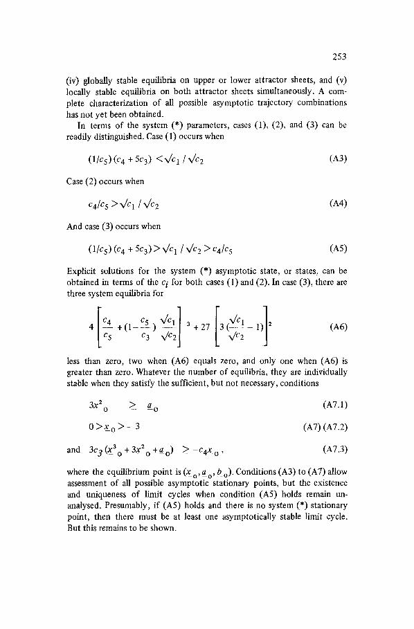
(iv) globally stable equilibria on upper or lower attractor sheets, and (v) locally stable equilibria on both attractor sheets simultaneously. A complete characterization of all possible asymptotic trajectory combinations has not yet been obtained.

In terms of the system (*) parameters, cases (1), (2), and (3) can be readily distinguished. Case (1) occurs when

(1/C5)(c 4 + 5c3) <~/C 1 /~/c 2 (A3)

Case (2) occurs when

c4/c 5 >~/c 1 / ~/c 2 (A4)

And case (3) occurs when

(1/c5) (c 4 + 5c3) > N/c 1 / ~/c 2 > c4/c 5 (A5)

Explicit solutions for the system (*) asymptotic state, or states, can be obtained in terms of the c i for both cases (1) and (2). In case (3), there are three system equilibria for

I c4 C5 ~/C- 1 ] I ( ~ C l ) ] 4 + ( 1 - - c 5 ) 3 +27 3 - 1 2 c3 4c2j

(A6)

less than zero, two when (A6) equals zero, and only one when (A6) is greater than zero. Whatever the number of equilibria, they are individually stable when they satisfy the sufficient, but not necessary, conditions

3X2o > --a o (A7 .1 )

0 >x_ o > - 3 (A7) (A7.2)

and 3c 3 (x__3 o + 3x2 o +a_o) > - c 4 x O , (A7.3)

where the equilibrium point is (x o, a o, b o). Conditions (A3) to (A7) allow assessment of all possible asymptotic stationary points, but the existence and uniqueness of limit cycles when condition (A5) holds remain un- analysed. Presumably, if (A5) holds and there is no system (*) stationary point, then there must be at least one asymptotically stable limit cycle. But this remains to be shown.

Documents

Ecological outbreak dynamics and the cusp catastrophe