ECON 3010Intermediate Macroeconomics

Chapter 5Inflation:

Its Causes, Effects, and Social Costs

0%

2%

4%

6%

8%

10%

12%

1960 1965 1970 1975 1980 1985 1990 1995 2000 2005 2010

% c

hang

e fro

m 1

2 m

os. e

arlie

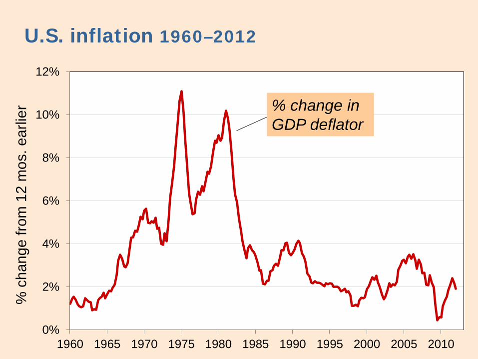
rU.S. inflation 1960–2012

% change in GDP deflator

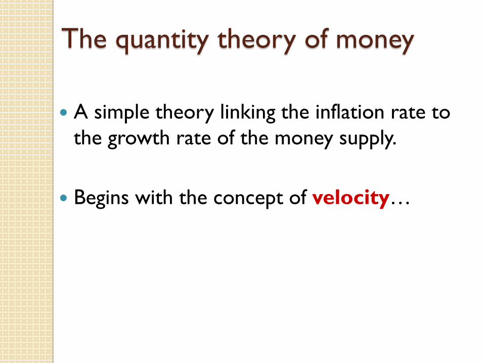
The quantity theory of money

A simple theory linking the inflation rate to the growth rate of the money supply.

Begins with the concept of velocity…

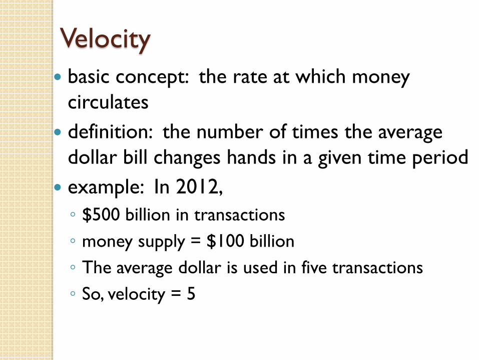
Velocity basic concept: the rate at which money

circulates definition: the number of times the average

dollar bill changes hands in a given time period example: In 2012, ◦ $500 billion in transactions◦ money supply = $100 billion◦ The average dollar is used in five transactions◦ So, velocity = 5

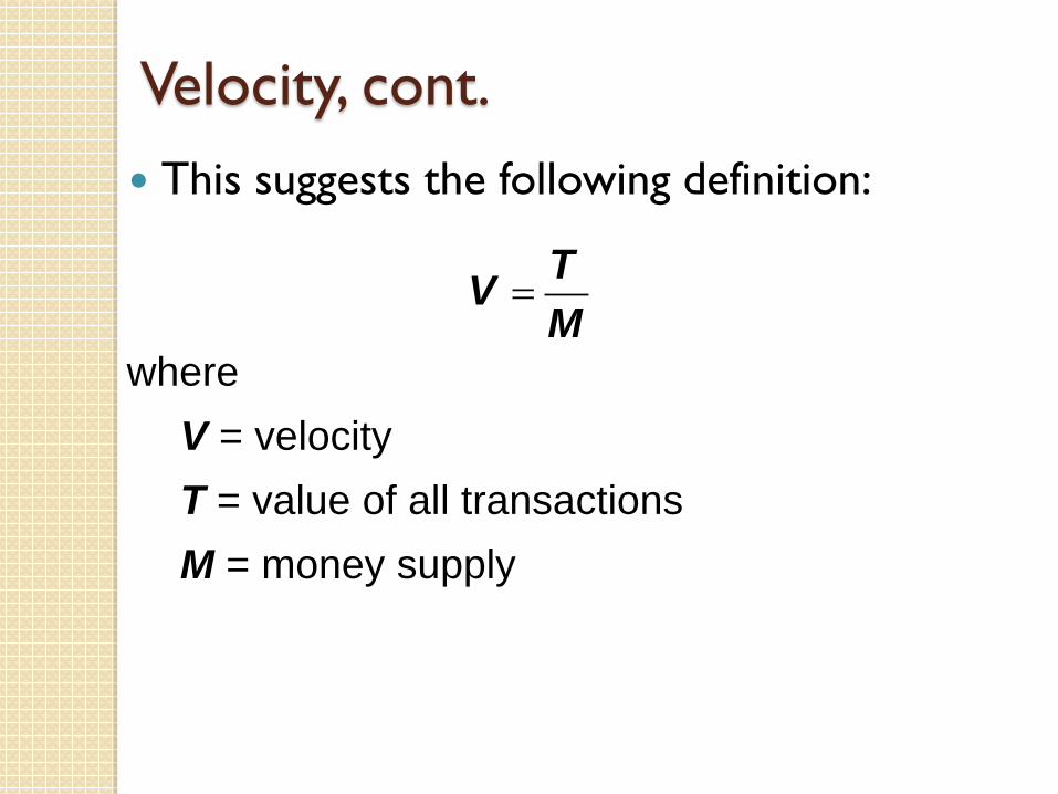
Velocity, cont. This suggests the following definition:

TVM

=

where V = velocityT = value of all transactionsM = money supply

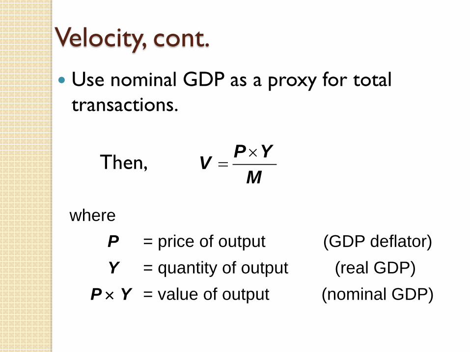
Velocity, cont. Use nominal GDP as a proxy for total

transactions.

Then, P YVM×

=

whereP = price of output (GDP deflator)Y = quantity of output (real GDP)

P × Y = value of output (nominal GDP)

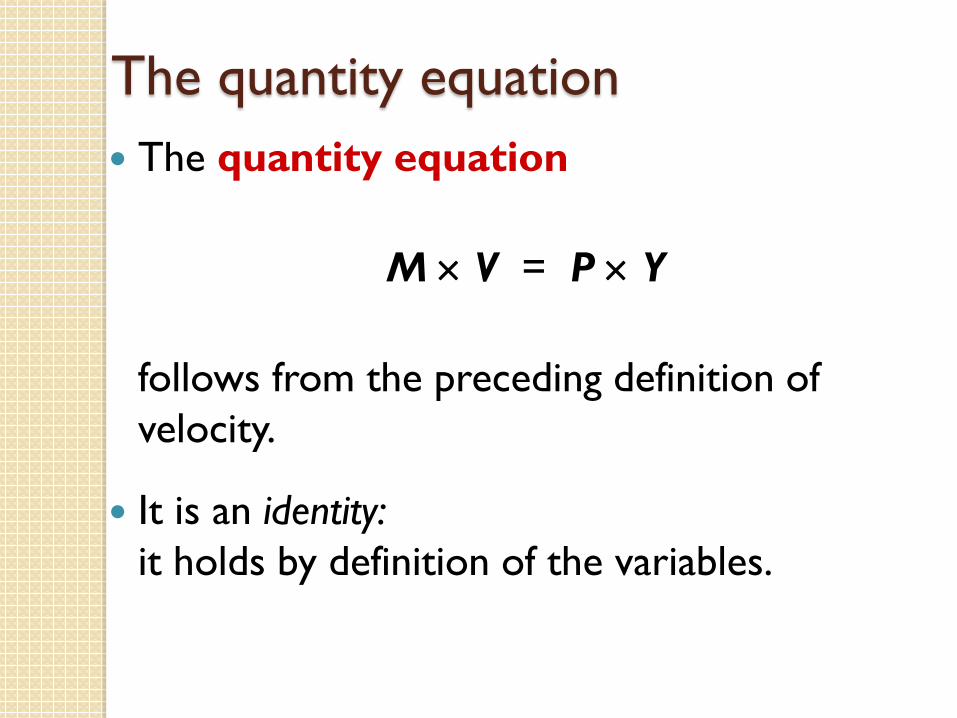
The quantity equation The quantity equation

M × V = P × Y

follows from the preceding definition of velocity.

It is an identity:it holds by definition of the variables.

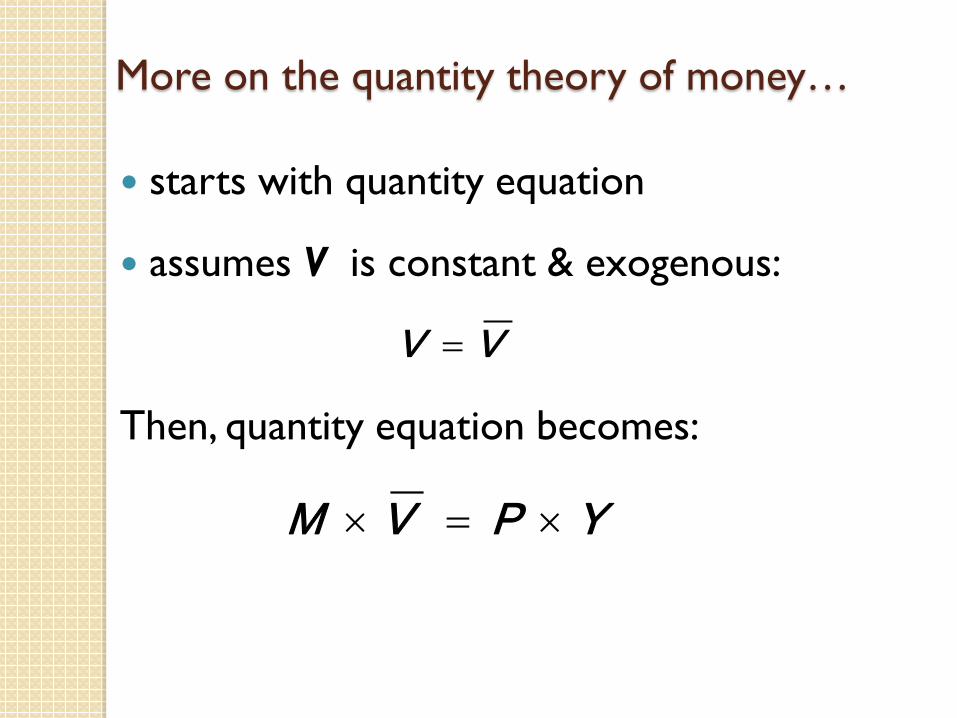
More on the quantity theory of money…

starts with quantity equation

assumes V is constant & exogenous:

Then, quantity equation becomes:

=V V

× = ×M V P Y

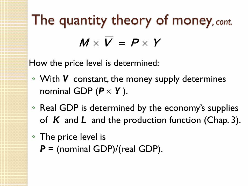
The quantity theory of money, cont.

How the price level is determined:

◦ With V constant, the money supply determines nominal GDP (P × Y ).

◦ Real GDP is determined by the economy’s supplies of K and L and the production function (Chap. 3).

◦ The price level is P = (nominal GDP)/(real GDP).

× = ×M V P Y

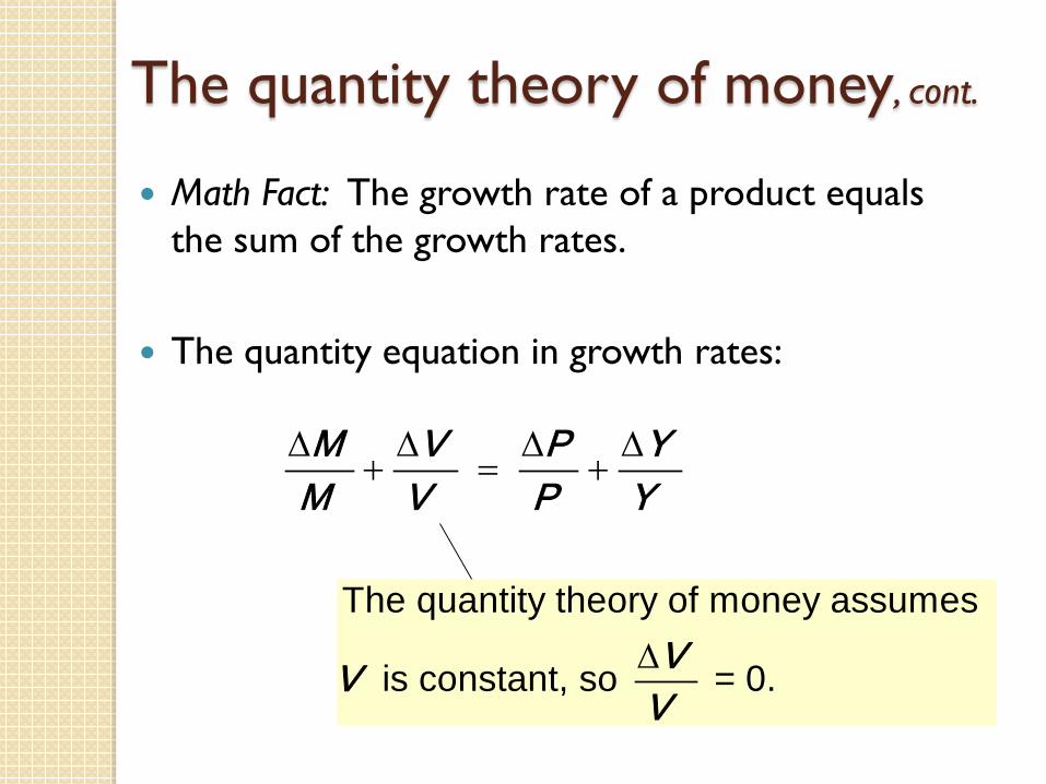
The quantity theory of money, cont.

Math Fact: The growth rate of a product equals the sum of the growth rates.

The quantity equation in growth rates:

M V P YM V P Y∆ ∆ ∆ ∆

+ = +

The quantity theory of money assumes

is constant, so = 0.∆VVV

The quantity theory of money, cont.

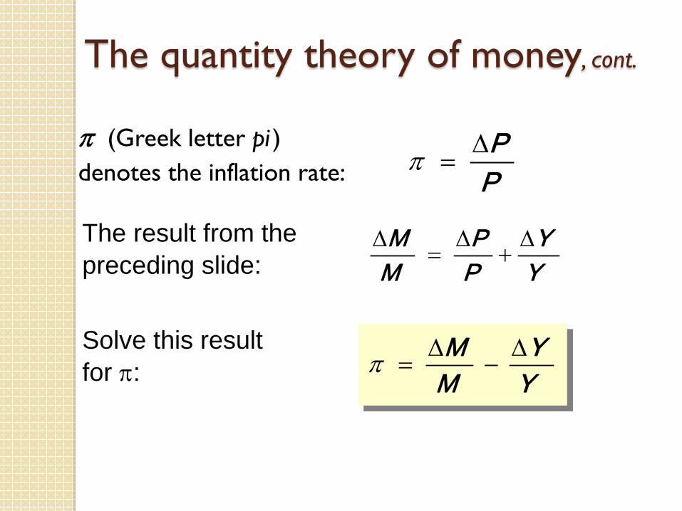
π (Greek letter pi ) denotes the inflation rate:

M P YM P Y∆ ∆ ∆

= +

PP∆

=π

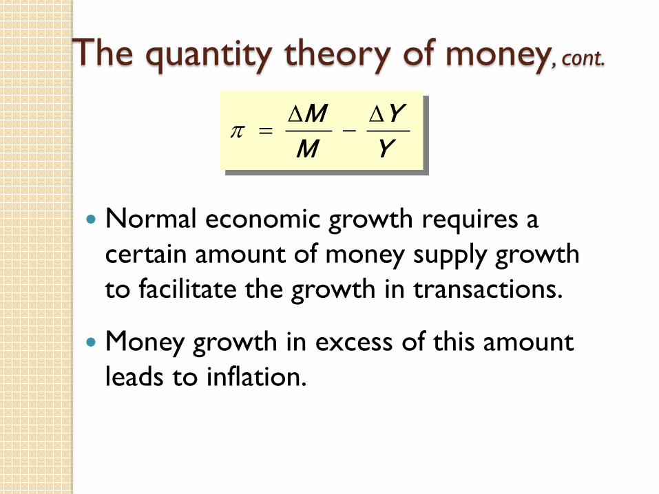
π ∆ ∆= −

M YM Y

The result from the preceding slide:

Solve this result for π:

The quantity theory of money, cont.

Normal economic growth requires a certain amount of money supply growth to facilitate the growth in transactions.

Money growth in excess of this amount leads to inflation.

π ∆ ∆= −

M YM Y

Confronting the quantity theory with data

The quantity theory of money implies:

1. Countries with higher money growth rates should have higher inflation rates.

2. The long-run trend in a country’s inflation rate should be similar to the long-run trend in the country’s money growth rate.

Are the data consistent with these implications?

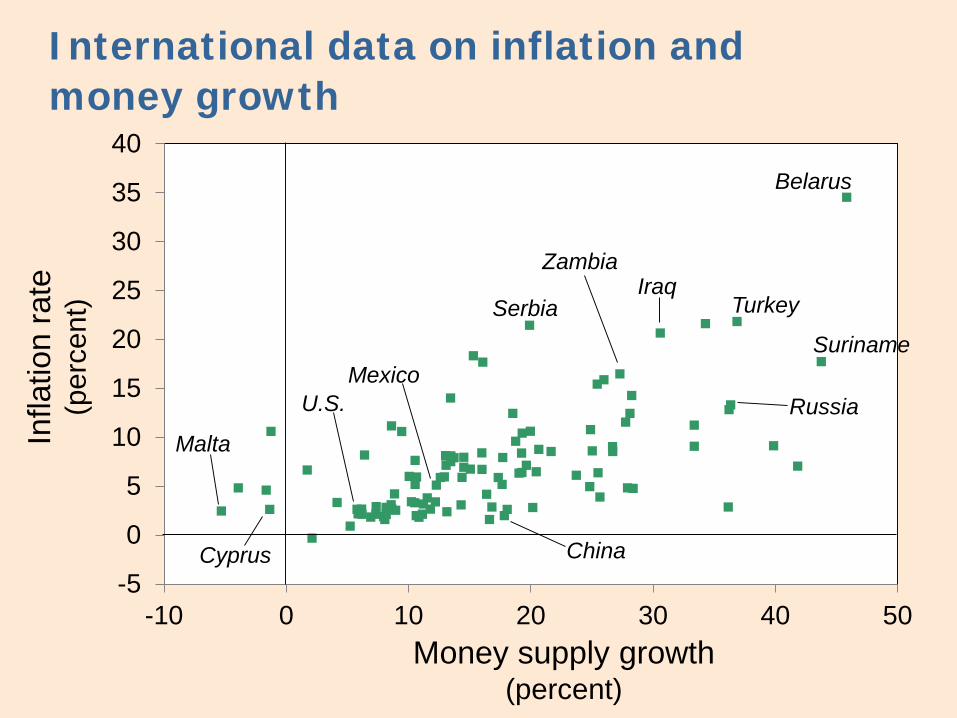
International data on inflation and money growth

Infla

tion

rate

(p

erce

nt)

Money supply growth(percent)

-5

0

5

10

15

20

25

30

35

40

-10 0 10 20 30 40 50

China

IraqTurkey

Belarus

Zambia

U.S.Mexico

Malta

Cyprus

SerbiaSuriname

Russia

0%

2%

4%

6%

8%

10%

12%

14%

1960 1965 1970 1975 1980 1985 1990 1995 2000 2005 2010

% c

hang

e fro

m 1

2 m

os. e

arlie

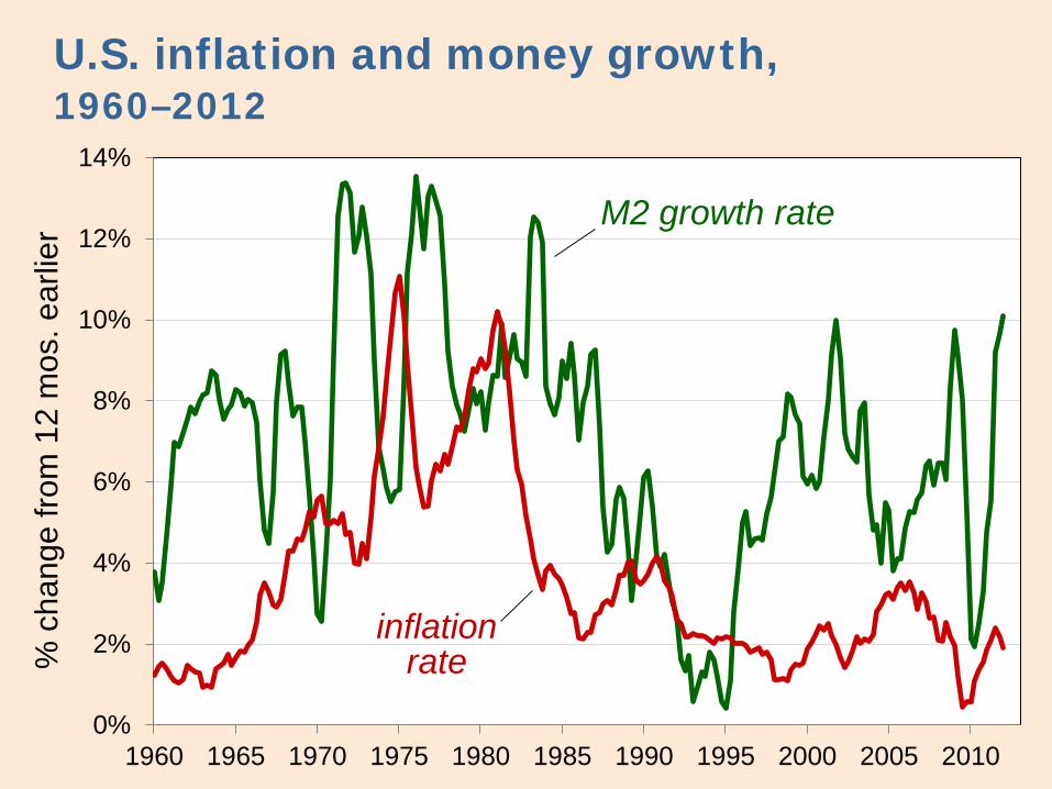
rU.S. inflation and money growth, 1960–2012

M2 growth rate

inflation rate

0%

2%

4%

6%

8%

10%

12%

14%

1960 1965 1970 1975 1980 1985 1990 1995 2000 2005 2010

% c

hang

e fro

m 1

2 m

os. e

arlie

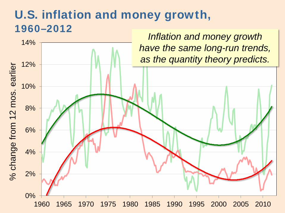
rU.S. inflation and money growth, 1960–2012

Inflation and money growth have the same long-run trends, as the quantity theory predicts.

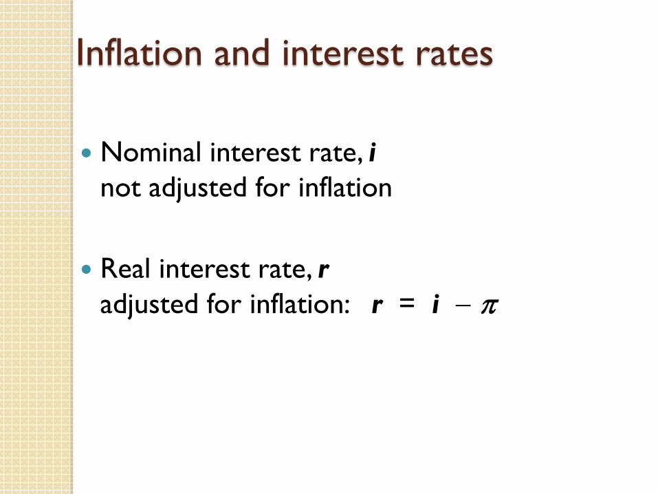
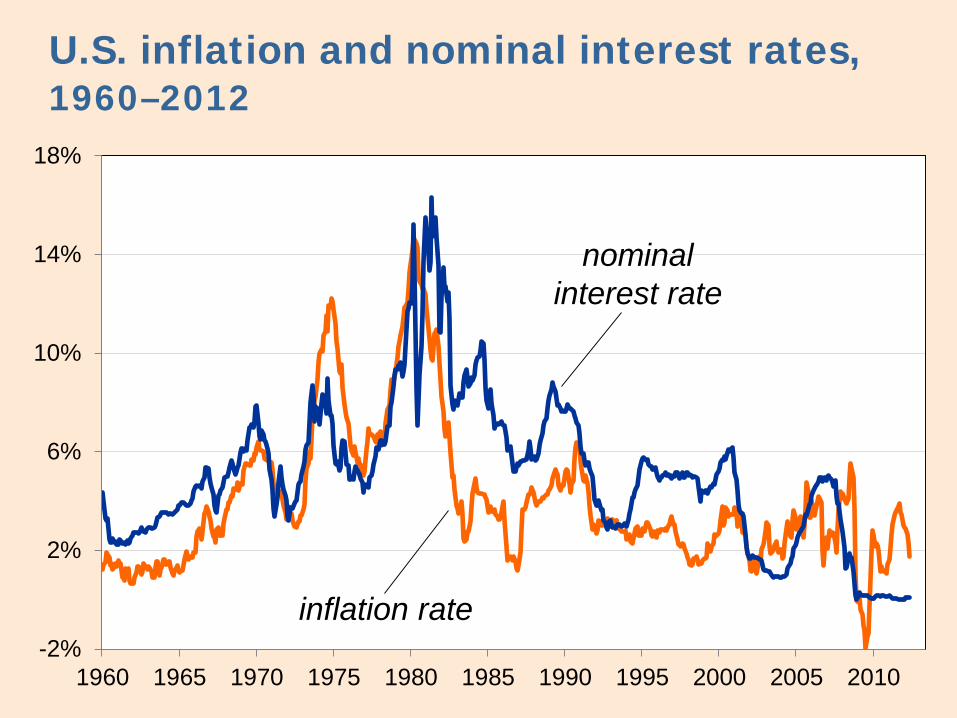
Inflation and interest rates

Nominal interest rate, inot adjusted for inflation

Real interest rate, radjusted for inflation: r = i − π

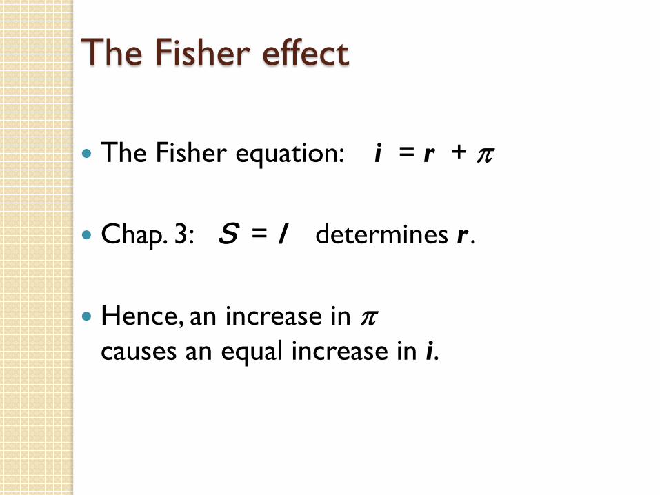
The Fisher effect

The Fisher equation: i = r + π

Chap. 3: S = I determines r .

Hence, an increase in πcauses an equal increase in i.

-2%

2%

6%

10%

14%

18%

1960 1965 1970 1975 1980 1985 1990 1995 2000 2005 2010

U.S. inflation and nominal interest rates, 1960–2012

inflation rate

nominal interest rate

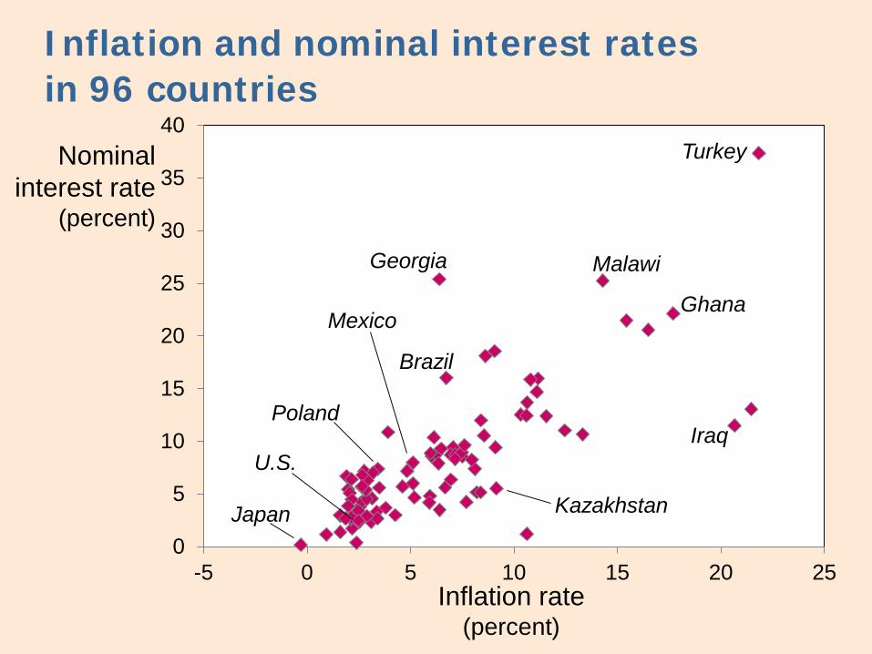
Inflation and nominal interest rates in 96 countries

Nominal interest rate

(percent)

Inflation rate(percent)

0

5

10

15

20

25

30

35

40

-5 0 5 10 15 20 25

MalawiGeorgia

Turkey

Ghana

IraqU.S.

Poland

Japan

Brazil

Kazakhstan

Mexico

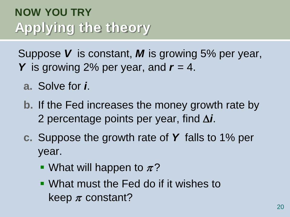
NOW YOU TRYApplying the theory

Suppose V is constant, M is growing 5% per year, Y is growing 2% per year, and r = 4.

a. Solve for i. b. If the Fed increases the money growth rate by

2 percentage points per year, find ∆i.c. Suppose the growth rate of Y falls to 1% per

year. What will happen to π? What must the Fed do if it wishes to

keep π constant?20

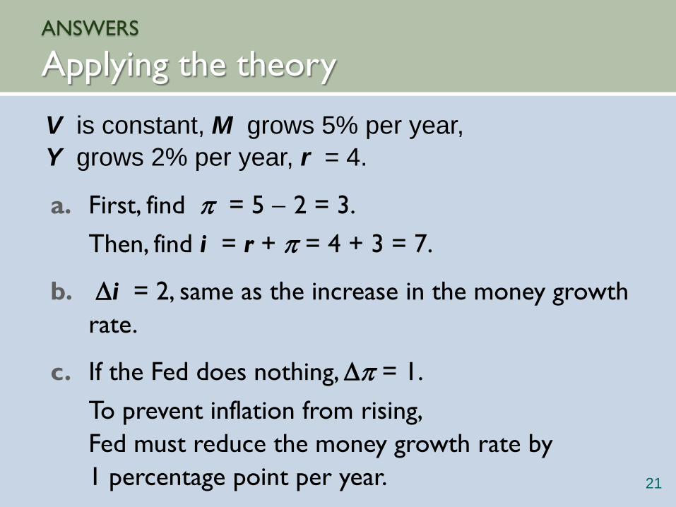
ANSWERS

Applying the theory

a. First, find π = 5 − 2 = 3. Then, find i = r + π = 4 + 3 = 7.

b. ∆i = 2, same as the increase in the money growth rate.

c. If the Fed does nothing, ∆π = 1. To prevent inflation from rising, Fed must reduce the money growth rate by 1 percentage point per year. 21

V is constant, M grows 5% per year, Y grows 2% per year, r = 4.

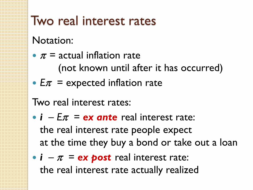
Two real interest ratesNotation: π = actual inflation rate

(not known until after it has occurred) Eπ = expected inflation rate

Two real interest rates: i – Eπ = ex ante real interest rate:

the real interest rate people expect at the time they buy a bond or take out a loan

i – π = ex post real interest rate:the real interest rate actually realized

Why is inflation bad?

Common misperception: inflation reduces real wages

This is true only in the short run, when nominal wages are fixed by contracts.

(Chap. 3) In the long run, the real wage is determined by labor supply and the marginal product of labor, not the price level or inflation rate.

Consider the data…

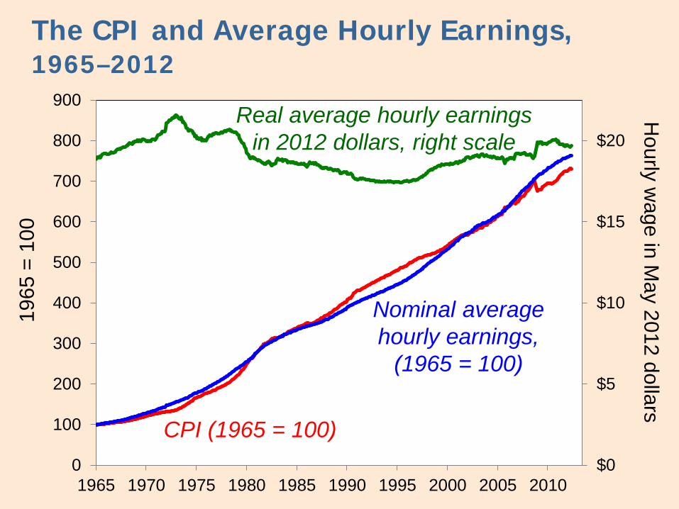
The CPI and Average Hourly Earnings, 1965–2012

1965

= 1

00H

ourly wage in M

ay 2012 dollars

$0

$5

$10

$15

$20

0

100

200

300

400

500

600

700

800

900

1965 1970 1975 1980 1985 1990 1995 2000 2005 2010

Real average hourly earnings in 2012 dollars, right scale

Nominal average hourly earnings,

(1965 = 100)

CPI (1965 = 100)

The classical view of inflation

The classical view: A change in the price level is merely a change in the units of measurement.

Then, why is inflation a social problem?

The social costs of inflation

…fall into two categories:

1. costs when inflation is expected2. costs when inflation is different than

people had expected

The costs of expected inflation: Shoeleather cost def: the costs and inconveniences of reducing money

balances to avoid the inflation tax.

↑π ⇒ ↑i⇒ ↓ real money balances

So, same monthly spending but lower average money holdings means more frequent trips to the bank to withdraw smaller amounts of cash.

The costs of expected inflation: Menu costs

def: The costs of changing prices.

Examples:◦ cost of printing new menus◦ cost of printing & mailing new catalogs

The higher is inflation, the more frequently firms must change their prices and incur these costs.

The costs of expected inflation: Relative price distortions

Firms facing menu costs change prices infrequently.

Different firms change their prices at different times, leading to relative price distortions……causing microeconomic inefficiencies in the allocation of resources.

The costs of expected inflation: Unfair tax treatmentSome taxes are not adjusted to account for inflation, such as the capital gains tax.

Example:

◦ Jan 1: you buy $10,000 worth of IBM stock

◦ Dec 31: you sell the stock for $11,000, so your nominal capital gain is $1,000 (10%).

◦ Suppose π = 10% during the year. Your real capital gain is $0.

◦ But the govt requires you to pay taxes on your $1,000 nominal gain!!

The costs of expected inflation: General inconvenience

Inflation makes it harder to compare nominal values from different time periods.

This complicates long-range financial planning.

Additional cost of unexpected inflation: Arbitrary redistribution of purchasing power

Many long-term contracts not indexed, but based on Eπ .

If π turns out different from Eπ , then some gain at others’ expense.

Example: borrowers & lenders ◦ If π > Eπ , then purchasing power is transferred

from lenders to borrowers.◦ If π < Eπ , then purchasing power is transferred

from borrowers to lenders.

Additional cost of high inflation: Increased uncertainty

When inflation is high, it’s more variable and unpredictable: π is different from Eπ more often, and the differences tend to be larger

So, arbitrary redistributions of wealth more likely.

This creates higher uncertainty, making risk-averse people worse off.

One benefit of inflation

Nominal wages are rarely reduced. This hinders labor market clearing.

Inflation allows the real wages to reach equilibrium levels without nominal wage cuts.

Therefore, moderate inflation improves the functioning of labor markets.

The Classical Dichotomy Classical dichotomy:

the separation of real and nominal variables in the classical model, which implies nominal variables do not affect real variables.

Neutrality of money: Changes in the money supply do not affect real variables. In the real world, money is approximately neutral in the long run.