Economic Cost-Benefit Analysis: Padma Bridge Project · Economic Cost-Benefit Analysis: Padma Bridge Project Bangladesh Priorities Ashikur Rahman Senior Economist, Policy Research

Benefits and Costs of Completing the Padma Bridge

ECONOMIC COST-BENEFIT ANALYSIS: PADMA BRIDGE PROJECT

ASHIKUR RAHMAN, SENIOR ECONOMIST, POLICY RESEARCH INSTITUTE (PRI) OF BANGLADESHBAZLUL HAQUE KHONDKER, PROFESSOR, DEPARTMENT OF ECONOMICS, UNIVERSITY OF DHAKA

Economic Cost-Benefit Analysis: Padma Bridge Project

Bangladesh Priorities

Ashikur Rahman Senior Economist, Policy Research Institute (PRI) of Bangladesh

Bazlul Haque Khondker Professor, Department of Economics, University of Dhaka

© 2016 Copenhagen Consensus Center [email protected] www.copenhagenconsensus.com This work has been produced as a part of the Bangladesh Priorities project, a collaboration between Copenhagen Consensus Center and BRAC Research and Evaluation Department. The Bangladesh Priorities project was made possible by a generous grant from the C&A Foundation. Some rights reserved

This work is available under the Creative Commons Attribution 4.0 International license (CC BY 4.0). Under the Creative Commons Attribution license, you are free to copy, distribute, transmit, and adapt this work, including for commercial purposes, under the following conditions:

Attribution Please cite the work as follows: #AUTHOR NAME#, #PAPER TITLE#, Bangladesh Priorities, Copenhagen Consensus Center, 2016. License: Creative Commons Attribution CC BY 4.0.

Third-party-content Copenhagen Consensus Center does not necessarily own each component of the content contained within the work. If you wish to re-use a component of the work, it is your responsibility to determine whether permission is needed for that re-use and to obtain permission from the copyright owner. Examples of components can include, but are not limited to, tables, figures, or images.

mailto:[email protected]

http://www.copenhagenconsensus.com/

http://creativecommons.org/licenses/by/4.0/

1

INTRODUCTION AND BACKGROUND................................................................................................................ 2

OVERVIEW OF THE PREVIOUS ECONOMIC BENEFIT COST ANALYSIS ................................................................ 2

TRAFFIC AND REVENUE FORECASTS ................................................................................................................. 6

COST ESCALATION ........................................................................................................................................... 7

DATA AND METHODOLOGY ............................................................................................................................. 9

BENEFIT-COST ANALYSIS ................................................................................................................................ 12

CONCLUDING OBSERVATIONS ....................................................................................................................... 14

ANNEX 1: TRAFFIC AND REVENUE FORECASTS ............................................................................................................. 20

ANNEX 2: VEHICLE OPERATING COSTS AND TRAVEL TIME COSTS .................................................................................... 20

SOURCE: “ROAD USER COST ANNUAL REPORT FOR 2004-05”, ROADS AND HIGHWAYS DEPARTMENTANNEX 3: ESTIMATED ROAD

USERS BENEFIT – TRAFFIC MODEL ............................................................................................................................ 20

ANNEX 4: DESCRIPTION OF THE SAM MODEL AND ESTIMATED ECONOMY WIDE BENEFIT .................................................. 23

2

Introduction and Background

The construction of Padma Bridge will provide road and rail links between the relatively less-developed

Southwest region (SWR) of the country and the more-developed eastern half that includes the capital

of Dhaka and the port city of Chittagong. By facilitating transportation across the river, the bridge is

expected to lead to a greater integration of regional markets within the Bangladeshi national economy.

It is also expected that the Padma Bridge will have the most significant economic and poverty impacts

in Khulna and Barisal Divisions – the southwest region of Bangladesh. Given its importance to the

Bangladesh economy several studies were conducted to assess the project cost, expected benefit and

finally the financial and economic feasibility applying conventional measures such as NPV, IRR and BCR.

One of such study was commissioned by the Bangladesh Bridge Authority in 2010 with financial

assistance from the World Bank. In additional to the conventional benefit derived from a traffic model,

the study assessed the economy wide benefit of the Padma Bridge and concluded on the basis of three

measures of benefit-cost analysis that the Padma Bridger project would be financially viable. The donor

consortium withdrew their funding of the project on corruption charges. Bangladesh government then

decided to fund the project from their own funding. As a result of uncertainty over funding, the project

could not be started and accordingly the completion of the project deadline has been shifted from 2015

to 2018. According to Bridges Division, the delay led to rise of the project cost by three times. This paper

tries to reassess the feasibility of the Padma Bridge project against the backdrop of increasing project

costs.

The rest of the paper is composed of five more sections. Section two provides an overview of the

previous benefit cost analysis. Cost escalation has been discussed in section three. Data and

methodology has been discussed in section four. Section five presents benefit-cost analysis. Final

section provides concluding observations.

Overview of the Previous Economic Benefit Cost Analysis1

Raihan and Khondker (2010) used four different types of methodologies to quantify the economic as

well as welfare implication of Padma Bridge. Although strict comparisons of the outcomes of these

1 Benefit cost analysis refers to a study conducted in 2010 by Raihan and Khondker. For details please see “Estimating the Economic Impacts of the Padma Bridge in Bangladesh”. The study was commissioned by the Bangladesh Bridge Authority and the World Bank.

3

models are not usually advocated, they have been used in the study to examine the robustness of the

project benefit outcomes2.

a) Although, it is customary to use ‘traffic’ models to estimate the economic benefits of transport

project (e.g. Padma Bridge), reliance only on the traffic model may underestimate full benefits

of the project since such model can only capture primary or direct benefit in the form of

efficiency gains arising out of cost and time saved.

b) The secondary benefits of a transportation project are also substantial. The secondary effects

may be generated due to multi-sectoral productivity gain through structural change occurring

in the economy from improved productivity made possible by the bridge. The well known

models for capturing secondary benefits are SAM based fixed price and CGE models.

c) Hence in addition to adopting the traffic model, both SAM based fixed price and CGE models

are employed to estimate full benefits of the Padma Bridge project. In this context the full

benefits would thus compose of efficiency gains of traffic model and the economy wide

benefits of the SAM and CGE models.

d) Because of its location in the South West region of Bangladesh, Padma Bridge is expected to

have larger impacts on this regions compared to the other parts of Bangladesh. A regional CGE

model, although not an impossibility, has not been possible because of lack of required region

specific parameters and elasticity values. However a regional SAM model was formulated to

assess the impacts of Padma Bridge on the SW region of Bangladesh.

Estimated Benefits

1. In the Traffic model, road users benefits are estimated based on the saving on vehicle operation

costs (VOC) and savings in travel time cost (TTC). Total road user benefit is estimated to be about

million 1,295,840 taka ($18,512 million) over the 31 year period3. The economic benefits are on top

of the financial benefits estimated using the forecasted traffic volume and levying of toll (please

see section 3).

2 All these models are stand alone model and hence their outcomes should be considered independent of each other. Strict comparison is not advocated in the literature. However, in this exercise road user benefit of the traffic model is combined with the outcome of the SAM model (i.e. considering it as a measure of economy wide secondary impacts due to the implementation of the project) to derive total benefit of the project. 3 The quantifiable cost and benefits of the Padma Bridge carried out by AECOM New Zealand Limited. For details please see “Padma Multipurpose Bridge Design Project: Detailed Economic and Financial Analysis- Revision 1”, AECOM New Zealand Limited.

4

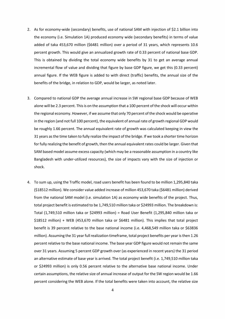
2. As for economy-wide (secondary) benefits, use of national SAM with injection of $2.1 billion into

the economy (i.e. Simulation 1A) produced economy wide (secondary benefits) in terms of value

added of taka 453,670 million ($6481 million) over a period of 31 years, which represents 10.6

percent growth. This would give an annualized growth rate of 0.33 percent of national base GDP.

This is obtained by dividing the total economy wide benefits by 31 to get an average annual

incremental flow of value and dividing that figure by base GDP figure, we get this (0.33 percent)

annual figure. If the WEB figure is added to with direct (traffic) benefits, the annual size of the

benefits of the bridge, in relation to GDP, would be larger, as noted later.

3. Compared to national GDP the average annual increase in SW regional base GDP because of WEB

alone will be 2.3 percent. This is on the assumption that a 100 percent of the shock will occur within

the regional economy. However, if we assume that only 70 percent of the shock would be operative

in the region (and not full 100 percent), the equivalent of annual rate of growth regional GDP would

be roughly 1.66 percent. The annual equivalent rate of growth was calculated keeping in view the

31 years as the time taken to fully realize the impact of the bridge. If we took a shorter time horizon

for fully realizing the benefit of growth, then the annual equivalent rates could be larger. Given that

SAM based model assume excess capacity (which may be a reasonable assumption in a country like

Bangladesh with under-utilized resources), the size of impacts vary with the size of injection or

shock.

4. To sum up, using the Traffic model, road users benefit has been found to be million 1,295,840 taka

($18512 million). We consider value added increase of million 453,670 taka ($6481 million) derived

from the national SAM model (i.e. simulation 1A) as economy wide benefits of the project. Thus,

total project benefit is estimated to be 1,749,510 million taka or $24993 million. The breakdown is:

Total (1,749,510 million taka or $24993 million) = Road User Benefit (1,295,840 million taka or

$18512 million) + WEB (453,670 million taka or $6481 million). This implies that total project

benefit is 39 percent relative to the base national income (i.e. 4,468,549 million taka or $63836

million). Assuming the 31 year full realization timeframe, total project benefits per year is then 1.26

percent relative to the base national income. The base year GDP figure would not remain the same

over 31 years. Assuming 5 percent GDP growth over (as experienced in recent years) the 31 period

an alternative estimate of base year is arrived. The total project benefit (i.e. 1,749,510 million taka

or $24993 million) is only 0.56 percent relative to the alternative base national income. Under

certain assumptions, the relative size of annual increase of output for the SW region would be 1.66

percent considering the WEB alone. If the total benefits were taken into account, the relative size

5

of annual flow of benefits in comparison to regional GDP would, of course, be larger and, would

depend on how much of the traffic benefits would accrue to the south-west region.

5. Further assessment of the total project benefits (explained above) in terms of conventional project

appraisal measures suggests that the project is economically viable. More specifically, the project

is viable with:

a net present value4 of US$ 1234 million;

a benefit-cost ratio (BCR) of 2.01;

an economic internal rate of return (EIRR) of 19 percent.

6. The application of constrained optimization model such as CGE model outcomes also vindicates the

findings of the traffic model and SAM based model. More specifically, 50 percent reduction in

transport margins may lead to welfare increase by 0.78 percent compared to the base value.

Furthermore, conventional project appraisal measures inclusive of CGE outcome suggest that the

project is also economically viable. The conventional project appraisal measures with CGE outcome

are:

a net present value of US$ 851 million;

a benefit-cost ratio (BCR) of 1.72;

an economic internal rate of return (EIRR) of 17 percent.

7. Under certain assumptions, the construction of the Padma Bridge would lead to an annualised

reduction in head-count poverty at the national level by 0.84 percent and at the regional level by

1.01 percent. Other simulations also indicated reduction in poverty in different magnitudes.

4 A discount rate of 12% was used in the BCR calculation.

6

Traffic and Revenue Forecasts5

A transport model was developed by AECOM to forecasts traffic volume and revenues on the Padma

Bridge. The calibration of the model was done using detailed information on socio-economic and

travel patterns. Some of the key parameters and variables include:

I. Changed land use patterns;

II. Changed population and number of households;

III. Regional and national economic growth;

IV. Growth in car ownership;

V. Increase in value of time; and

When the forecasting exercise was conducted it was projected that opening year traffic (2014) would

be 12,000 vehicles per day, growing over 63,000 in thirty years at a growth rate of 6.3% per annum.

AECOM argued that “initially, trucks and buses make up around 75% of vehicles on Padma Bridge,

although light vehicles (cars and motorcycles) make up an increasing proportion of traffic as vehicle

ownership in Bangladesh increases. Thus, the change in traffic mix results in a slightly lower long term

growth rate of revenue around 5.8%”.

They further stated that “by 2036, traffic volumes on Padma Bridge are assumed to be close to

capacity, given current capacity assumptions and vehicle technology. The forecasts have therefore

been capped at 75,000 vehicles per day. Further, as traffic using Padma Bridge will be additional to

existing local traffic, capacity on the N8 to Dhaka will require upgrading to at least four lanes. This was

assumed to occur from year of opening. Between the western end of the bridge and Bhanga junction,

it was assumed that the N8 is widened by 2025 to four lanes”.

5 AECOM (2010), ‘Padma Multipurpose Bridge Design Project: Detailed Economic and Financial Analysis’, Revision 1 Bangladesh Bridge Authority, 11 February 2010. AECOM New Zealand Limited

7

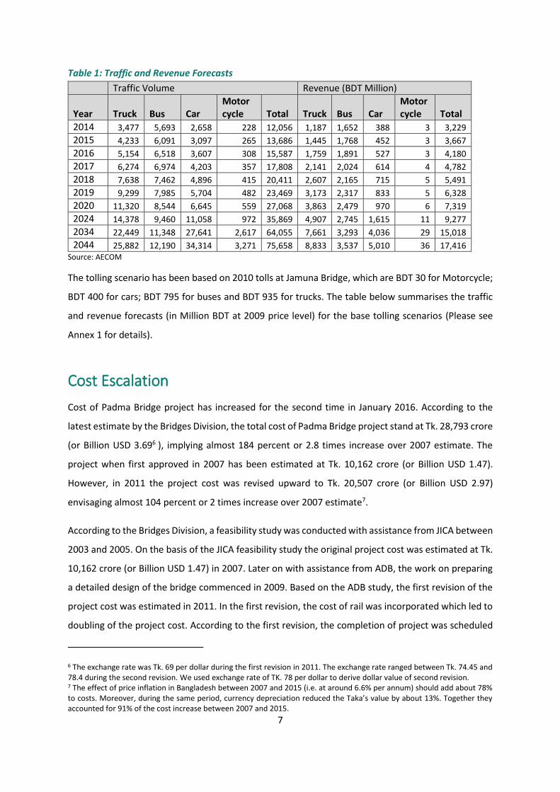
Table 1: Traffic and Revenue Forecasts

Traffic Volume Revenue (BDT Million)

Year Truck Bus Car Motor cycle Total Truck Bus Car

Motor cycle Total

2014 3,477 5,693 2,658 228 12,056 1,187 1,652 388 3 3,229

2015 4,233 6,091 3,097 265 13,686 1,445 1,768 452 3 3,667

2016 5,154 6,518 3,607 308 15,587 1,759 1,891 527 3 4,180

2017 6,274 6,974 4,203 357 17,808 2,141 2,024 614 4 4,782

2018 7,638 7,462 4,896 415 20,411 2,607 2,165 715 5 5,491

2019 9,299 7,985 5,704 482 23,469 3,173 2,317 833 5 6,328

2020 11,320 8,544 6,645 559 27,068 3,863 2,479 970 6 7,319

2024 14,378 9,460 11,058 972 35,869 4,907 2,745 1,615 11 9,277

2034 22,449 11,348 27,641 2,617 64,055 7,661 3,293 4,036 29 15,018

2044 25,882 12,190 34,314 3,271 75,658 8,833 3,537 5,010 36 17,416 Source: AECOM

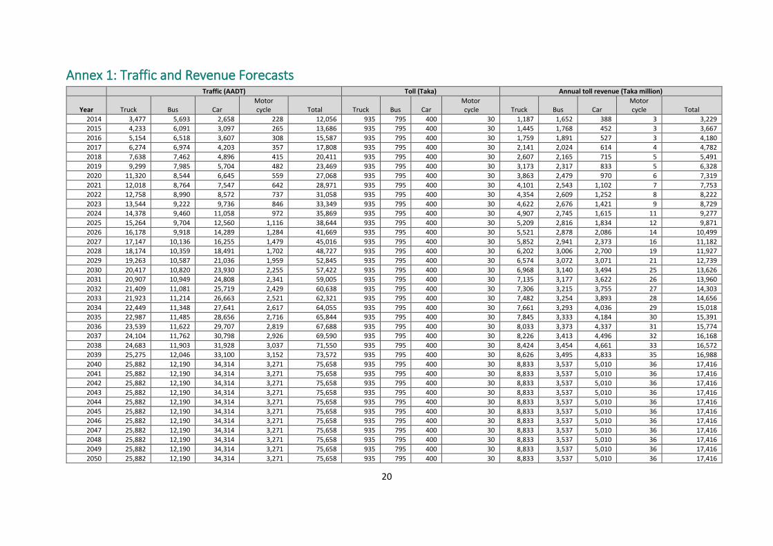
The tolling scenario has been based on 2010 tolls at Jamuna Bridge, which are BDT 30 for Motorcycle;

BDT 400 for cars; BDT 795 for buses and BDT 935 for trucks. The table below summarises the traffic

and revenue forecasts (in Million BDT at 2009 price level) for the base tolling scenarios (Please see

Annex 1 for details).

Cost Escalation

Cost of Padma Bridge project has increased for the second time in January 2016. According to the

latest estimate by the Bridges Division, the total cost of Padma Bridge project stand at Tk. 28,793 crore

(or Billion USD 3.696 ), implying almost 184 percent or 2.8 times increase over 2007 estimate. The

project when first approved in 2007 has been estimated at Tk. 10,162 crore (or Billion USD 1.47).

However, in 2011 the project cost was revised upward to Tk. 20,507 crore (or Billion USD 2.97)

envisaging almost 104 percent or 2 times increase over 2007 estimate7.

According to the Bridges Division, a feasibility study was conducted with assistance from JICA between

2003 and 2005. On the basis of the JICA feasibility study the original project cost was estimated at Tk.

10,162 crore (or Billion USD 1.47) in 2007. Later on with assistance from ADB, the work on preparing

a detailed design of the bridge commenced in 2009. Based on the ADB study, the first revision of the

project cost was estimated in 2011. In the first revision, the cost of rail was incorporated which led to

doubling of the project cost. According to the first revision, the completion of project was scheduled

6 The exchange rate was Tk. 69 per dollar during the first revision in 2011. The exchange rate ranged between Tk. 74.45 and 78.4 during the second revision. We used exchange rate of TK. 78 per dollar to derive dollar value of second revision. 7 The effect of price inflation in Bangladesh between 2007 and 2015 (i.e. at around 6.6% per annum) should add about 78% to costs. Moreover, during the same period, currency depreciation reduced the Taka’s value by about 13%. Together they accounted for 91% of the cost increase between 2007 and 2015.

8

for 2015. But recently the completion date has extended to 2018 which has also led to further

escalation of cost.

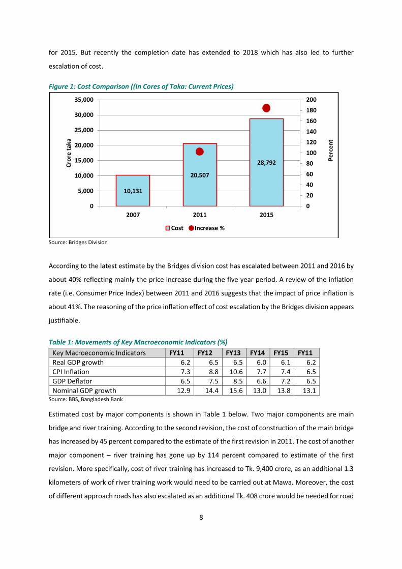
Figure 1: Cost Comparison ((In Cores of Taka: Current Prices)

Source: Bridges Division

According to the latest estimate by the Bridges division cost has escalated between 2011 and 2016 by

about 40% reflecting mainly the price increase during the five year period. A review of the inflation

rate (i.e. Consumer Price Index) between 2011 and 2016 suggests that the impact of price inflation is

about 41%. The reasoning of the price inflation effect of cost escalation by the Bridges division appears

justifiable.

Table 1: Movements of Key Macroeconomic Indicators (%)

Key Macroeconomic Indicators FY11 FY12 FY13 FY14 FY15 FY11

Real GDP growth 6.2 6.5 6.5 6.0 6.1 6.2

CPI Inflation 7.3 8.8 10.6 7.7 7.4 6.5

GDP Deflator 6.5 7.5 8.5 6.6 7.2 6.5

Nominal GDP growth 12.9 14.4 15.6 13.0 13.8 13.1 Source: BBS, Bangladesh Bank

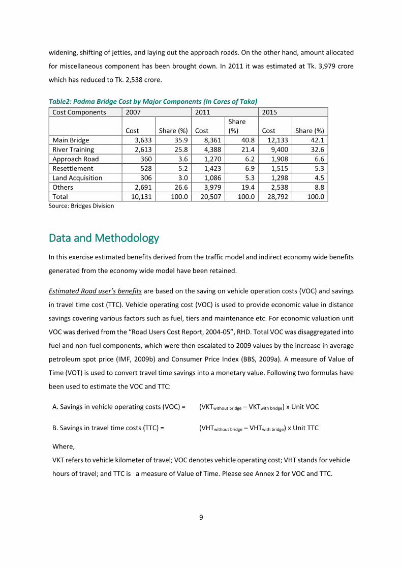
Estimated cost by major components is shown in Table 1 below. Two major components are main

bridge and river training. According to the second revision, the cost of construction of the main bridge

has increased by 45 percent compared to the estimate of the first revision in 2011. The cost of another

major component – river training has gone up by 114 percent compared to estimate of the first

revision. More specifically, cost of river training has increased to Tk. 9,400 crore, as an additional 1.3

kilometers of work of river training work would need to be carried out at Mawa. Moreover, the cost

of different approach roads has also escalated as an additional Tk. 408 crore would be needed for road

10,131

20,507

28,792

0

20

40

60

80

100

120

140

160

180

200

0

5,000

10,000

15,000

20,000

25,000

30,000

35,000

2007 2011 2015

Pe

rce

nt

Cro

re t

aka

Cost Increase %

9

widening, shifting of jetties, and laying out the approach roads. On the other hand, amount allocated

for miscellaneous component has been brought down. In 2011 it was estimated at Tk. 3,979 crore

which has reduced to Tk. 2,538 crore.

Table2: Padma Bridge Cost by Major Components (In Cores of Taka)

Cost Components 2007 2011 2015

Cost Share (%) Cost Share (%) Cost Share (%)

Main Bridge 3,633 35.9 8,361 40.8 12,133 42.1

River Training 2,613 25.8 4,388 21.4 9,400 32.6

Approach Road 360 3.6 1,270 6.2 1,908 6.6

Resettlement 528 5.2 1,423 6.9 1,515 5.3

Land Acquisition 306 3.0 1,086 5.3 1,298 4.5

Others 2,691 26.6 3,979 19.4 2,538 8.8

Total 10,131 100.0 20,507 100.0 28,792 100.0 Source: Bridges Division

Data and Methodology

In this exercise estimated benefits derived from the traffic model and indirect economy wide benefits

generated from the economy wide model have been retained.

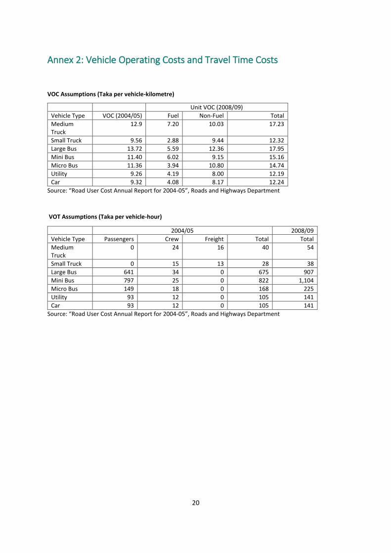
Estimated Road user’s benefits are based on the saving on vehicle operation costs (VOC) and savings

in travel time cost (TTC). Vehicle operating cost (VOC) is used to provide economic value in distance

savings covering various factors such as fuel, tiers and maintenance etc. For economic valuation unit

VOC was derived from the “Road Users Cost Report, 2004-05”, RHD. Total VOC was disaggregated into

fuel and non-fuel components, which were then escalated to 2009 values by the increase in average

petroleum spot price (IMF, 2009b) and Consumer Price Index (BBS, 2009a). A measure of Value of

Time (VOT) is used to convert travel time savings into a monetary value. Following two formulas have

been used to estimate the VOC and TTC:

A. Savings in vehicle operating costs (VOC) = (VKTwithout bridge – VKTwith bridge) x Unit VOC

B. Savings in travel time costs (TTC) = (VHTwithout bridge – VHTwith bridge) x Unit TTC

Where,

VKT refers to vehicle kilometer of travel; VOC denotes vehicle operating cost; VHT stands for vehicle

hours of travel; and TTC is a measure of Value of Time. Please see Annex 2 for VOC and TTC.

10

Savings in travel time costs account for 23% of total benefits estimated by Design Consultant. Unit

travel time costs for passengers and crew were sourced from RHD (2005) and for freight in transit

from STUP (2007). These were then escalated to 2009 using prices by estimated increase in General

Wage Rate Index from BBS (2008) and ADB (2009). These constitute a major part of the quantifiable

benefits. Total road user benefit is estimated to be about million 1,295,840 taka over the 31 year

period.

Although economic benefits of road users have been retained, the economy wide benefits (WEB) has

been re-estimated using national and regional social accounting matrices (SAM). Two scenarios have

been considered: (i) in simulation one (SIM 1) the fifty (50%) of the total cost will be used in the

domestic economy (e.g. foreign currency cost component is thus 50% - will be use outside implying a

leakage from the domestic economy); (ii) in simulation two (SIM 2) the only thirty (30%) of the total

cost will be used in the domestic economy (e.g. foreign currency cost is thus 70% - implying higher

leakage).

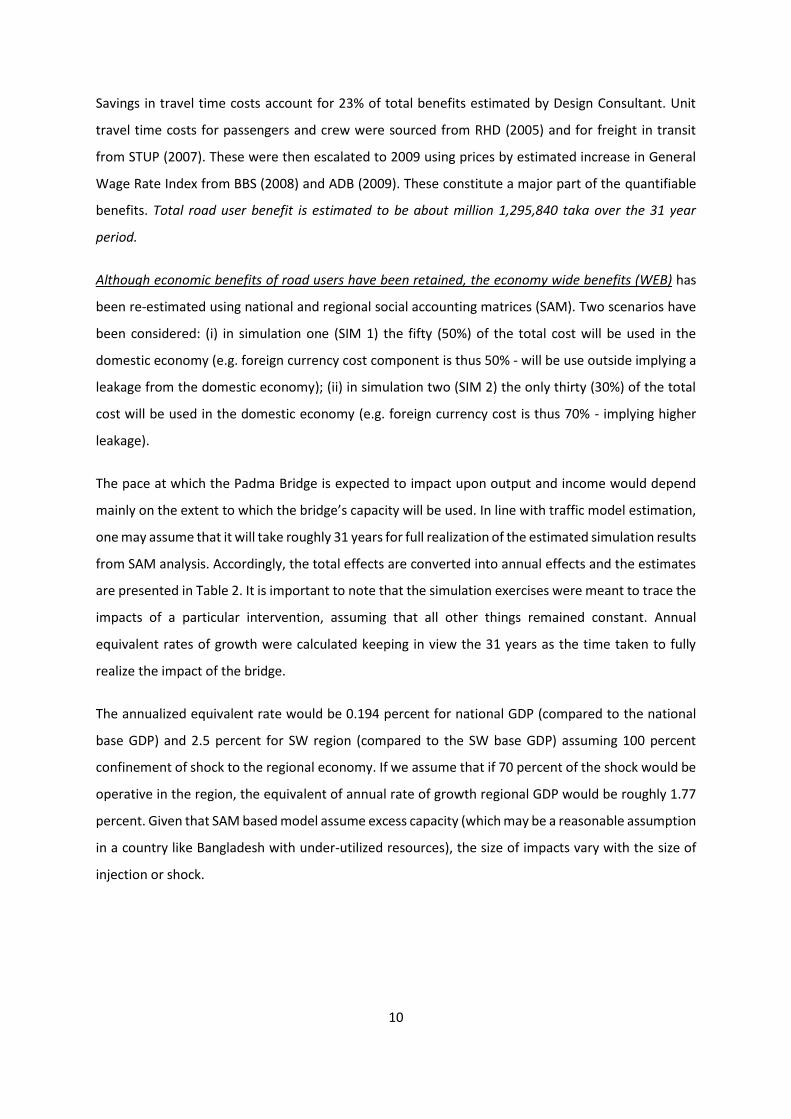
The pace at which the Padma Bridge is expected to impact upon output and income would depend

mainly on the extent to which the bridge’s capacity will be used. In line with traffic model estimation,

one may assume that it will take roughly 31 years for full realization of the estimated simulation results

from SAM analysis. Accordingly, the total effects are converted into annual effects and the estimates

are presented in Table 2. It is important to note that the simulation exercises were meant to trace the

impacts of a particular intervention, assuming that all other things remained constant. Annual

equivalent rates of growth were calculated keeping in view the 31 years as the time taken to fully

realize the impact of the bridge.

The annualized equivalent rate would be 0.194 percent for national GDP (compared to the national

base GDP) and 2.5 percent for SW region (compared to the SW base GDP) assuming 100 percent

confinement of shock to the regional economy. If we assume that if 70 percent of the shock would be

operative in the region, the equivalent of annual rate of growth regional GDP would be roughly 1.77

percent. Given that SAM based model assume excess capacity (which may be a reasonable assumption

in a country like Bangladesh with under-utilized resources), the size of impacts vary with the size of

injection or shock.

11

Table2: Total and Annualized Economy Wide Benefit of Simulations (% Change from Base Values)

Simulation 1A: National SAM Based

Simulation 1B: Regional SAM Based

Simulation 2A: National SAM Based

Simulation 2B: Regional SAM Based

Increase in: Total

(1) Annualized

(2) Total

(3) Annualized

(4) Total*

(5) Annualized

(6) Total

(7) Annualized

(8) Total

(9) Annualized

(10)

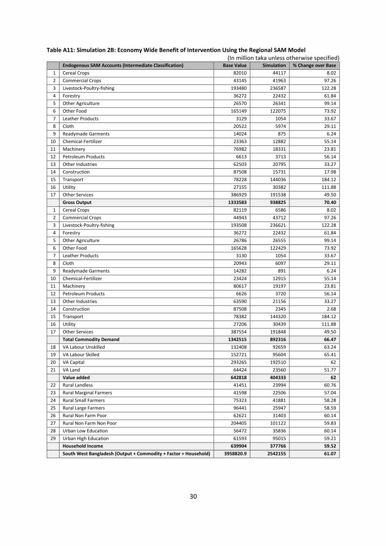
Gross Output 6.02 0.194 78.34 2.53 51.4 1.66 3.61 0.116 47.00 1.516 Commodity 5.85 0.188 78.23 2.51 51.3 1.66 3.51 0.113 46.94 1.514 Factor Return 5.79 0.187 76.16 2.46 49.9 1.61 3.48 0.112 45.68 1.474

Household Income 5.12 0.165 72.72 2.34 47.7 1.54

3.07 0.099 43.63 1.407

Note: Gross output = intermediate use + factor payments; Total commodity demand = commodity demanded by households; Value added = factor payments; Household income = Incomes of different household categories

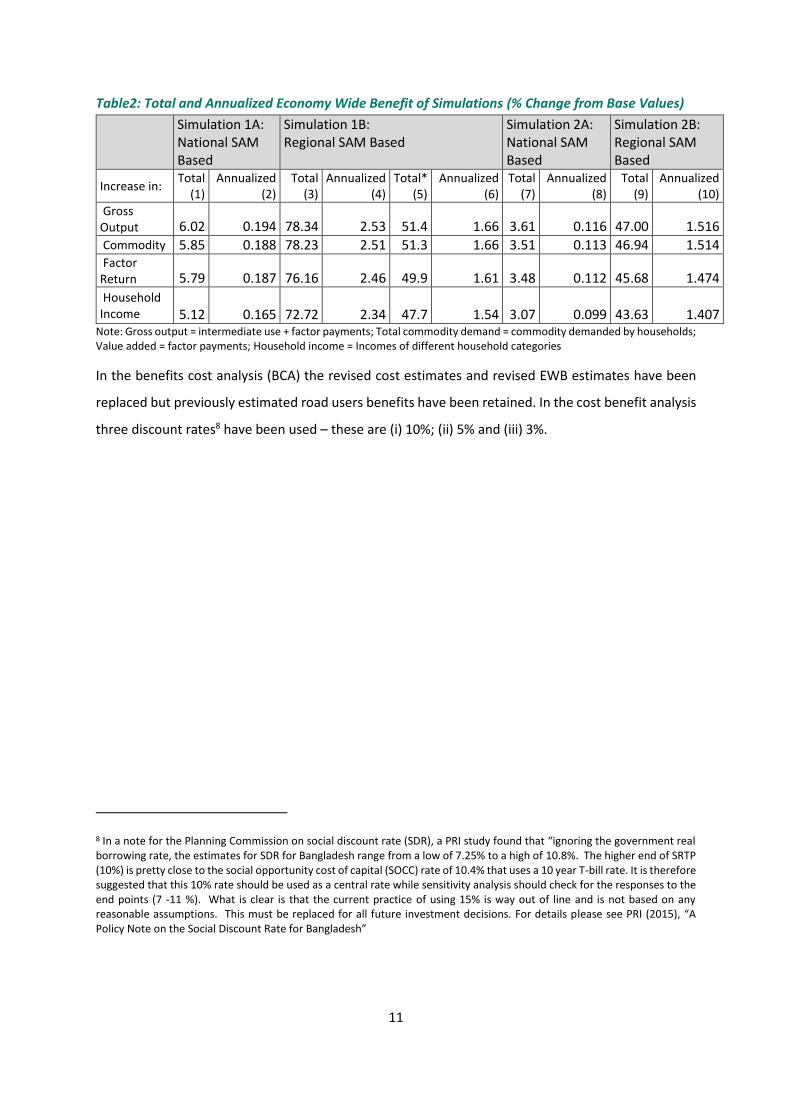
In the benefits cost analysis (BCA) the revised cost estimates and revised EWB estimates have been

replaced but previously estimated road users benefits have been retained. In the cost benefit analysis

three discount rates8 have been used – these are (i) 10%; (ii) 5% and (iii) 3%.

8 In a note for the Planning Commission on social discount rate (SDR), a PRI study found that “ignoring the government real borrowing rate, the estimates for SDR for Bangladesh range from a low of 7.25% to a high of 10.8%. The higher end of SRTP (10%) is pretty close to the social opportunity cost of capital (SOCC) rate of 10.4% that uses a 10 year T-bill rate. It is therefore suggested that this 10% rate should be used as a central rate while sensitivity analysis should check for the responses to the end points (7 -11 %). What is clear is that the current practice of using 15% is way out of line and is not based on any reasonable assumptions. This must be replaced for all future investment decisions. For details please see PRI (2015), “A Policy Note on the Social Discount Rate for Bangladesh”

12

Benefit-Cost Analysis

As mentioned above standard measure such as benefit cost ratio (BCR) has been used to assess the

feasibility of the Padma Bridge project. Assessment conducted in 2010 found benefit cost ratio of 2.01

for the Padma Bridge project.

In this exercise we have used to two estimated benefits (both direct and indirect). Under simulation

1, the total undiscounted benefits of the Padma Bridge have been estimated to be Tk. 1.8 trillion or

$22.4 billion. The breakdown is: Total (1.5 trillion taka or $22.4 billion) = Road User Benefit (1.3 trillion

taka or $18.5 billion) + WEB-SIM (0.3 trillion taka or $3.2 billion). On the other hand under under

simulation 2, the total undiscounted benefits of the Padma Bridge have been estimated to be Tk. 1.6

trillion or $21.1 billion. The breakdown is: Total (1.6 trillion taka or $21.4 billion) = Road User Benefit

(1.5 trillion taka or $18.5 billion) + WEB-SIM 2(0.1 trillion taka or $1.9 billion).

Road user’s benefits estimation were based on the saving on vehicle operation costs (VOC) and savings

in travel time cost (TTC). Vehicle operating cost (VOC) is used to provide economic value in distance


VOC was derived from the “Road Users Cost Report, 2004-05”, RHD. Compared to 2004-05 estimates,

although cost of some of these components may be increased such as tiers and maintenance but the

cost of fuel may have fallen leading a situation that economic valuation unit VOC more or less

remained unchanged. A measure of Value of Time (VOT) is used to convert travel time savings into a

monetary value. Savings in travel time costs account for 23% of total benefits estimated by Design

Consultant. Since, savings in travel would likely to remain same and total benefit has also remained

same (i.e. 2010 level), this component of Road user’s benefits would also likely to remain unchanged.

The cost of Padma Bridge has gone up by almost three times. The latest cost of $ 3.7bn has been

incorporated into the BCR framework to assess the feasibility of the Padma Bridge. It should be

important to note since in the exercise, escalated cost has been incorporated but benefits more or

less remained unchanged and hence may suggest an underestimation of BCR. The results of the

feasibility exercise with escalated costs and unchanged benefits are provided below.

13

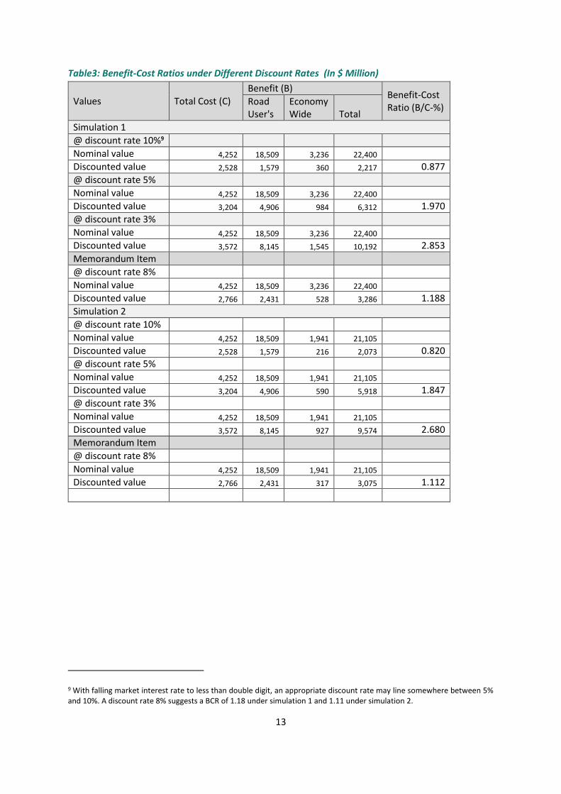
Table3: Benefit-Cost Ratios under Different Discount Rates (In $ Million)

Values Total Cost (C) Benefit (B)

Benefit-Cost Ratio (B/C-%)

Road User's

Economy Wide Total

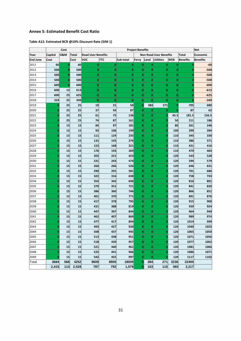
Simulation 1

@ discount rate 10%9

Nominal value 4,252 18,509 3,236 22,400

Discounted value 2,528 1,579 360 2,217 0.877

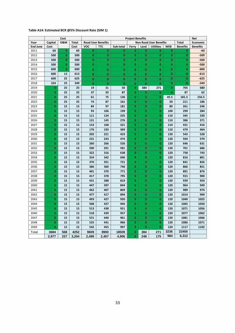
@ discount rate 5%

Nominal value 4,252 18,509 3,236 22,400


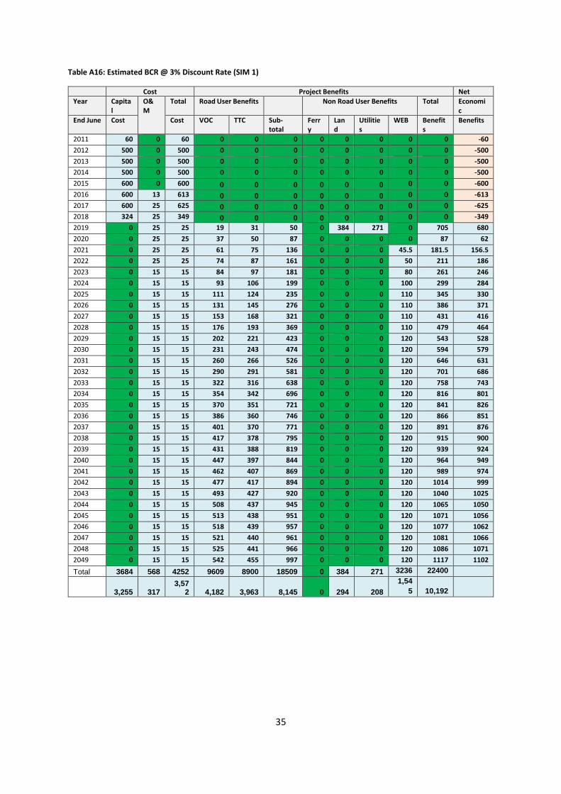
@ discount rate 3%

Nominal value 4,252 18,509 3,236 22,400

Discounted value 3,572 8,145 1,545 10,192 2.853

Memorandum Item

@ discount rate 8%

Nominal value 4,252 18,509 3,236 22,400


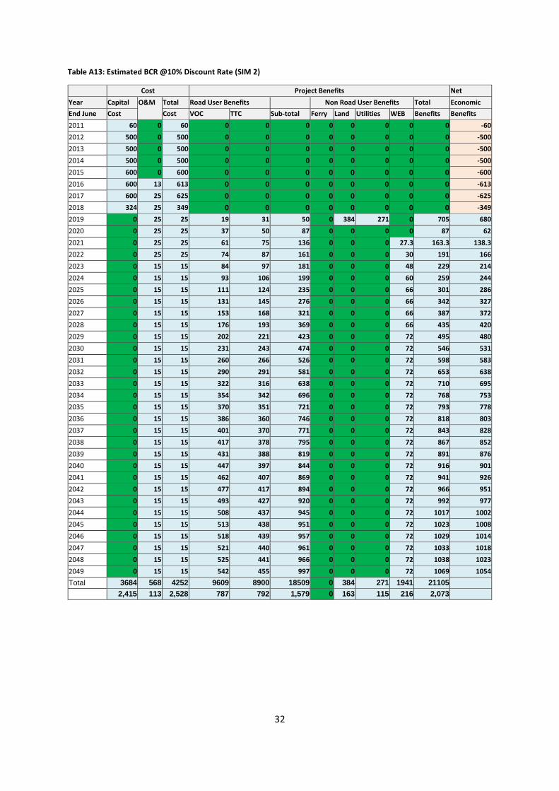
Simulation 2

@ discount rate 10%

Nominal value 4,252 18,509 1,941 21,105


@ discount rate 5%

Nominal value 4,252 18,509 1,941 21,105


@ discount rate 3%

Nominal value 4,252 18,509 1,941 21,105


Memorandum Item

@ discount rate 8%

Nominal value 4,252 18,509 1,941 21,105


9 With falling market interest rate to less than double digit, an appropriate discount rate may line somewhere between 5% and 10%. A discount rate 8% suggests a BCR of 1.18 under simulation 1 and 1.11 under simulation 2.

14

Concluding Observations

By facilitating transportation across the river, the Padma Bridge is expected lead to the greater

integration of regional markets within the Bangladeshi national economy. On the basis of their

suitability of capture primary and secondary economic impacts of construction project, three different

types of economy wide models are employed in addition to traditional traffic model to capture the total

and economy wide impacts of Padma Bridge.

In this exercise we have used to two estimated benefits (both direct and indirect). Under simulation

1, the total benefits of the Padma Bridge have been estimated to be Tk. 1,554,672 million or $21,747

million. The breakdown is: Total (1,554,672 million taka or $21,747 million) = Road User Benefit

(1,295,840 million taka or $18,512 million) + WEB-SIM 2(258,832 million taka or $3,235 million). On the

other under under simulation 2, the total benefits of the Padma Bridge have been estimated to be Tk.

1,451,139 million or $20,453 million. The breakdown is: Total (1,451,139 million taka or $20,453

million) = Road User Benefit (1,295,840 million taka or $18,512 million) + WEB-SIM 2(155,298 million

taka or $1,941 million). The latest project cost (i.e. 2016) has been incorporated into the benefit-cost

framework.

Three alternative discount rates (i.e. 10%; 5% and 3%) were used to assess to robustness of the

economic viability of the project.

Despite cost escalation by almost 3 times over the original estimate in 2007, the project would remain

viable according to the most of the revised BCR estimates. More specifically, BCR values of 0.887; 1.970;

and 2.853 respectively have been found for three alternative discount rates of 10%; 5% and 3% under

simulation 1. Upward adjustment of road users’ benefits would surely provide higher BCR values. For

instance, upward adjustment of unit VOC and TTT at 2015 prices would increase the BCR values to 1.127

and 1.070 respectively under SIM 1 and SIM 2 at 10 percent discount rate. Moreover, given the falling

market interest rate as an appropriate discount in Bangladesh now may lie somewhere between 5%

and 10%. Accordingly, use of discount rate 8% suggests a BCR of 1.18.

20

Annex 1: Traffic and Revenue Forecasts Traffic (AADT) Toll (Taka) Annual toll revenue (Taka million)

Year Truck Bus Car Motor cycle Total Truck Bus Car

Motor cycle Truck Bus Car

Motor cycle Total

2014 3,477 5,693 2,658 228 12,056 935 795 400 30 1,187 1,652 388 3 3,229

2015 4,233 6,091 3,097 265 13,686 935 795 400 30 1,445 1,768 452 3 3,667

2016 5,154 6,518 3,607 308 15,587 935 795 400 30 1,759 1,891 527 3 4,180

2017 6,274 6,974 4,203 357 17,808 935 795 400 30 2,141 2,024 614 4 4,782

2018 7,638 7,462 4,896 415 20,411 935 795 400 30 2,607 2,165 715 5 5,491

2019 9,299 7,985 5,704 482 23,469 935 795 400 30 3,173 2,317 833 5 6,328

2020 11,320 8,544 6,645 559 27,068 935 795 400 30 3,863 2,479 970 6 7,319

2021 12,018 8,764 7,547 642 28,971 935 795 400 30 4,101 2,543 1,102 7 7,753

2022 12,758 8,990 8,572 737 31,058 935 795 400 30 4,354 2,609 1,252 8 8,222

2023 13,544 9,222 9,736 846 33,349 935 795 400 30 4,622 2,676 1,421 9 8,729

2024 14,378 9,460 11,058 972 35,869 935 795 400 30 4,907 2,745 1,615 11 9,277

2025 15,264 9,704 12,560 1,116 38,644 935 795 400 30 5,209 2,816 1,834 12 9,871

2026 16,178 9,918 14,289 1,284 41,669 935 795 400 30 5,521 2,878 2,086 14 10,499

2027 17,147 10,136 16,255 1,479 45,016 935 795 400 30 5,852 2,941 2,373 16 11,182

2028 18,174 10,359 18,491 1,702 48,727 935 795 400 30 6,202 3,006 2,700 19 11,927

2029 19,263 10,587 21,036 1,959 52,845 935 795 400 30 6,574 3,072 3,071 21 12,739

2030 20,417 10,820 23,930 2,255 57,422 935 795 400 30 6,968 3,140 3,494 25 13,626

2031 20,907 10,949 24,808 2,341 59,005 935 795 400 30 7,135 3,177 3,622 26 13,960

2032 21,409 11,081 25,719 2,429 60,638 935 795 400 30 7,306 3,215 3,755 27 14,303

2033 21,923 11,214 26,663 2,521 62,321 935 795 400 30 7,482 3,254 3,893 28 14,656

2034 22,449 11,348 27,641 2,617 64,055 935 795 400 30 7,661 3,293 4,036 29 15,018

2035 22,987 11,485 28,656 2,716 65,844 935 795 400 30 7,845 3,333 4,184 30 15,391

2036 23,539 11,622 29,707 2,819 67,688 935 795 400 30 8,033 3,373 4,337 31 15,774

2037 24,104 11,762 30,798 2,926 69,590 935 795 400 30 8,226 3,413 4,496 32 16,168

2038 24,683 11,903 31,928 3,037 71,550 935 795 400 30 8,424 3,454 4,661 33 16,572

2039 25,275 12,046 33,100 3,152 73,572 935 795 400 30 8,626 3,495 4,833 35 16,988

2040 25,882 12,190 34,314 3,271 75,658 935 795 400 30 8,833 3,537 5,010 36 17,416

2041 25,882 12,190 34,314 3,271 75,658 935 795 400 30 8,833 3,537 5,010 36 17,416

2042 25,882 12,190 34,314 3,271 75,658 935 795 400 30 8,833 3,537 5,010 36 17,416

2043 25,882 12,190 34,314 3,271 75,658 935 795 400 30 8,833 3,537 5,010 36 17,416

2044 25,882 12,190 34,314 3,271 75,658 935 795 400 30 8,833 3,537 5,010 36 17,416

2045 25,882 12,190 34,314 3,271 75,658 935 795 400 30 8,833 3,537 5,010 36 17,416

2046 25,882 12,190 34,314 3,271 75,658 935 795 400 30 8,833 3,537 5,010 36 17,416

2047 25,882 12,190 34,314 3,271 75,658 935 795 400 30 8,833 3,537 5,010 36 17,416

2048 25,882 12,190 34,314 3,271 75,658 935 795 400 30 8,833 3,537 5,010 36 17,416

2049 25,882 12,190 34,314 3,271 75,658 935 795 400 30 8,833 3,537 5,010 36 17,416

2050 25,882 12,190 34,314 3,271 75,658 935 795 400 30 8,833 3,537 5,010 36 17,416

20

Annex 2: Vehicle Operating Costs and Travel Time Costs

VOC Assumptions (Taka per vehicle-kilometre)

Unit VOC (2008/09)

Vehicle Type VOC (2004/05) Fuel Non-Fuel Total

Medium Truck

12.9 7.20 10.03 17.23

Small Truck 9.56 2.88 9.44 12.32

Large Bus 13.72 5.59 12.36 17.95

Mini Bus 11.40 6.02 9.15 15.16

Micro Bus 11.36 3.94 10.80 14.74

Utility 9.26 4.19 8.00 12.19

Car 9.32 4.08 8.17 12.24

Source: “Road User Cost Annual Report for 2004-05”, Roads and Highways Department

VOT Assumptions (Taka per vehicle-hour)

2004/05 2008/09

Vehicle Type Passengers Crew Freight Total Total

Medium Truck

0 24 16 40 54

Small Truck 0 15 13 28 38

Large Bus 641 34 0 675 907

Mini Bus 797 25 0 822 1,104

Micro Bus 149 18 0 168 225

Utility 93 12 0 105 141

Car 93 12 0 105 141

Source: “Road User Cost Annual Report for 2004-05”, Roads and Highways Department

21

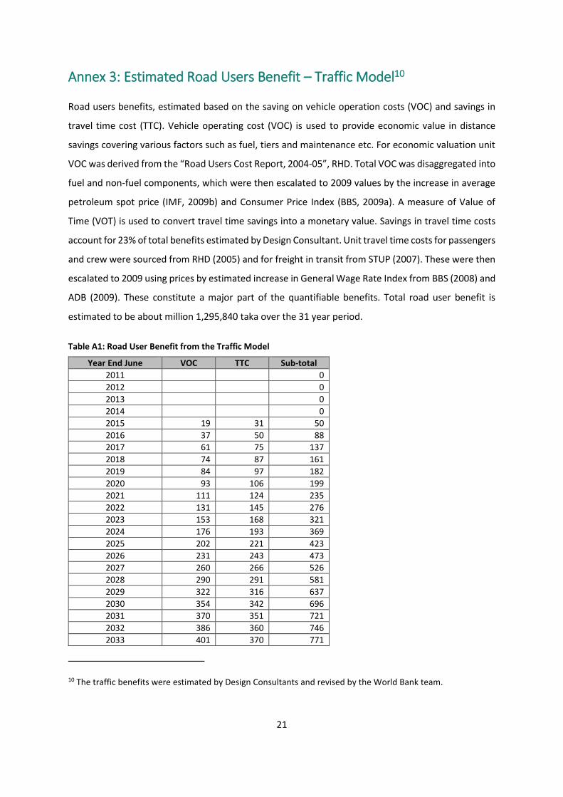
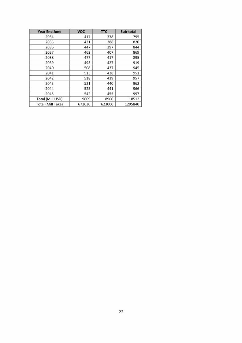
Annex 3: Estimated Road Users Benefit – Traffic Model10

Road users benefits, estimated based on the saving on vehicle operation costs (VOC) and savings in

travel time cost (TTC). Vehicle operating cost (VOC) is used to provide economic value in distance


VOC was derived from the “Road Users Cost Report, 2004-05”, RHD. Total VOC was disaggregated into

fuel and non-fuel components, which were then escalated to 2009 values by the increase in average

petroleum spot price (IMF, 2009b) and Consumer Price Index (BBS, 2009a). A measure of Value of

Time (VOT) is used to convert travel time savings into a monetary value. Savings in travel time costs

account for 23% of total benefits estimated by Design Consultant. Unit travel time costs for passengers

and crew were sourced from RHD (2005) and for freight in transit from STUP (2007). These were then

escalated to 2009 using prices by estimated increase in General Wage Rate Index from BBS (2008) and

ADB (2009). These constitute a major part of the quantifiable benefits. Total road user benefit is

estimated to be about million 1,295,840 taka over the 31 year period.

Table A1: Road User Benefit from the Traffic Model

Year End June VOC TTC Sub-total

2011 0

2012 0

2013 0

2014 0

2015 19 31 50

2016 37 50 88

2017 61 75 137

2018 74 87 161

2019 84 97 182

2020 93 106 199

2021 111 124 235

2022 131 145 276

2023 153 168 321

2024 176 193 369

2025 202 221 423

2026 231 243 473

2027 260 266 526

2028 290 291 581

2029 322 316 637

2030 354 342 696

2031 370 351 721

2032 386 360 746

2033 401 370 771

10 The traffic benefits were estimated by Design Consultants and revised by the World Bank team.

22

Year End June VOC TTC Sub-total

2034 417 378 795

2035 431 388 820

2036 447 397 844

2037 462 407 869

2038 477 417 895

2039 493 427 919

2040 508 437 945

2041 513 438 951

2042 518 439 957

2043 521 440 962

2044 525 441 966

2045 542 455 997

Total (Mill USD) 9609 8900 18512

Total (Mill Taka) 672630 623000 1295840

23

Annex 4:

Description of the SAM Model and Estimated Economy Wide Benefit

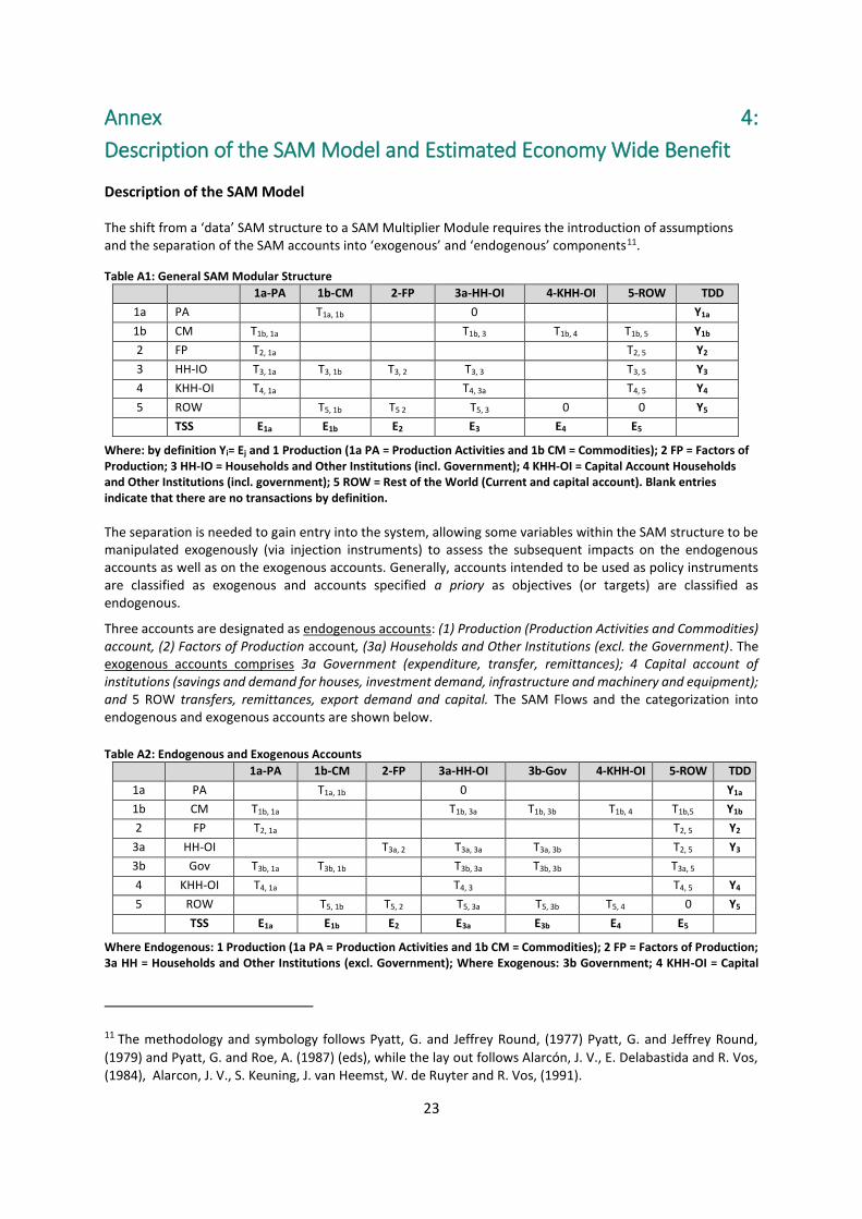
Description of the SAM Model

The shift from a ‘data’ SAM structure to a SAM Multiplier Module requires the introduction of assumptions and the separation of the SAM accounts into ‘exogenous’ and ‘endogenous’ components11.

Table A1: General SAM Modular Structure

1a-PA 1b-CM 2-FP 3a-HH-OI 4-KHH-OI 5-ROW TDD

1a PA T1a, 1b 0 Y1a

1b CM T1b, 1a T1b, 3 T1b, 4 T1b, 5 Y1b

2 FP T2, 1a T2, 5 Y2

3 HH-IO T3, 1a T3, 1b T3, 2 T3, 3 T3, 5 Y3

4 KHH-OI T4, 1a T4, 3a T4, 5 Y4

5 ROW T5, 1b T5 2 T5, 3 0 0 Y5

TSS E1a E1b E2 E3 E4 E5

Where: by definition Yi= Ej and 1 Production (1a PA = Production Activities and 1b CM = Commodities); 2 FP = Factors of Production; 3 HH-IO = Households and Other Institutions (incl. Government); 4 KHH-OI = Capital Account Households and Other Institutions (incl. government); 5 ROW = Rest of the World (Current and capital account). Blank entries indicate that there are no transactions by definition.

The separation is needed to gain entry into the system, allowing some variables within the SAM structure to be manipulated exogenously (via injection instruments) to assess the subsequent impacts on the endogenous accounts as well as on the exogenous accounts. Generally, accounts intended to be used as policy instruments are classified as exogenous and accounts specified a priory as objectives (or targets) are classified as endogenous.

Three accounts are designated as endogenous accounts: (1) Production (Production Activities and Commodities) account, (2) Factors of Production account, (3a) Households and Other Institutions (excl. the Government). The exogenous accounts comprises 3a Government (expenditure, transfer, remittances); 4 Capital account of institutions (savings and demand for houses, investment demand, infrastructure and machinery and equipment); and 5 ROW transfers, remittances, export demand and capital. The SAM Flows and the categorization into endogenous and exogenous accounts are shown below.

Table A2: Endogenous and Exogenous Accounts

1a-PA 1b-CM 2-FP 3a-HH-OI 3b-Gov 4-KHH-OI 5-ROW TDD

1a PA T1a, 1b 0 Y1a

1b CM T1b, 1a T1b, 3a T1b, 3b T1b, 4 T1b,5 Y1b

2 FP T2, 1a T2, 5 Y2

3a HH-OI T3a, 2 T3a, 3a T3a, 3b T2, 5 Y3

3b Gov T3b, 1a T3b, 1b T3b, 3a T3b, 3b T3a, 5

4 KHH-OI T4, 1a T4, 3 T4, 5 Y4

5 ROW T5, 1b T5, 2 T5, 3a T5, 3b T5, 4 0 Y5

TSS E1a E1b E2 E3a E3b E4 E5

Where Endogenous: 1 Production (1a PA = Production Activities and 1b CM = Commodities); 2 FP = Factors of Production; 3a HH = Households and Other Institutions (excl. Government); Where Exogenous: 3b Government; 4 KHH-OI = Capital

11 The methodology and symbology follows Pyatt, G. and Jeffrey Round, (1977) Pyatt, G. and Jeffrey Round,

(1979) and Pyatt, G. and Roe, A. (1987) (eds), while the lay out follows Alarcón, J. V., E. Delabastida and R. Vos, (1984), Alarcon, J. V., S. Keuning, J. van Heemst, W. de Ruyter and R. Vos, (1991).

24

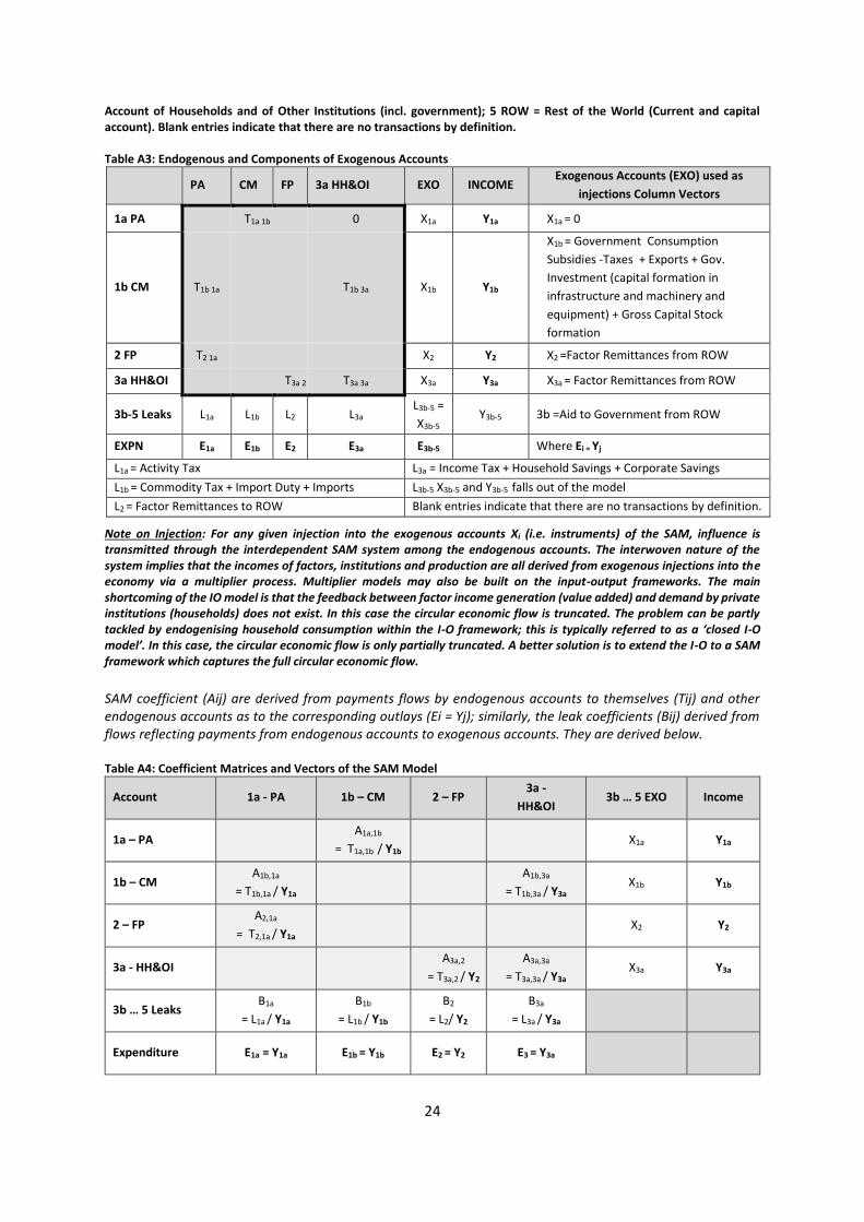
Account of Households and of Other Institutions (incl. government); 5 ROW = Rest of the World (Current and capital account). Blank entries indicate that there are no transactions by definition. Table A3: Endogenous and Components of Exogenous Accounts

PA CM FP 3a HH&OI EXO INCOME Exogenous Accounts (EXO) used as

injections Column Vectors

1a PA T1a 1b 0 X1a Y1a X1a = 0

1b CM T1b 1a T1b 3a X1b Y1b

X1b = Government Consumption

Subsidies -Taxes + Exports + Gov.

Investment (capital formation in

infrastructure and machinery and

equipment) + Gross Capital Stock

formation

2 FP T2 1a X2 Y2 X2 =Factor Remittances from ROW

3a HH&OI T3a 2 T3a 3a X3a Y3a X3a = Factor Remittances from ROW

3b-5 Leaks L1a L1b L2 L3a L3b-5 =

X3b-5 Y3b-5 3b =Aid to Government from ROW

EXPN E1a E1b E2 E3a E3b-5 Where Ei = Yj

L1a = Activity Tax L3a = Income Tax + Household Savings + Corporate Savings

L1b = Commodity Tax + Import Duty + Imports L3b-5 X3b-5 and Y3b-5 falls out of the model

L2 = Factor Remittances to ROW Blank entries indicate that there are no transactions by definition.

Note on Injection: For any given injection into the exogenous accounts Xi (i.e. instruments) of the SAM, influence is transmitted through the interdependent SAM system among the endogenous accounts. The interwoven nature of the system implies that the incomes of factors, institutions and production are all derived from exogenous injections into the economy via a multiplier process. Multiplier models may also be built on the input-output frameworks. The main shortcoming of the IO model is that the feedback between factor income generation (value added) and demand by private institutions (households) does not exist. In this case the circular economic flow is truncated. The problem can be partly tackled by endogenising household consumption within the I-O framework; this is typically referred to as a ‘closed I-O model’. In this case, the circular economic flow is only partially truncated. A better solution is to extend the I-O to a SAM framework which captures the full circular economic flow.

SAM coefficient (Aij) are derived from payments flows by endogenous accounts to themselves (Tij) and other endogenous accounts as to the corresponding outlays (Ei = Yj); similarly, the leak coefficients (Bij) derived from flows reflecting payments from endogenous accounts to exogenous accounts. They are derived below. Table A4: Coefficient Matrices and Vectors of the SAM Model

Account 1a - PA 1b – CM 2 – FP 3a -

HH&OI 3b … 5 EXO Income

1a – PA A1a,1b

= T1a,1b / Y1b X1a Y1a

1b – CM A1b,1a

= T1b,1a / Y1a

A1b,3a

= T1b,3a / Y3a X1b Y1b

2 – FP A2,1a

= T2,1a / Y1a X2 Y2

3a - HH&OI A3a,2

= T3a,2 / Y2

A3a,3a

= T3a,3a / Y3a X3a Y3a

3b … 5 Leaks B1a

= L1a / Y1a

B1b

= L1b / Y1b

B2

= L2/ Y2

B3a

= L3a / Y3a

Expenditure E1a = Y1a E1b = Y1b E2 = Y2 E3 = Y3a

25

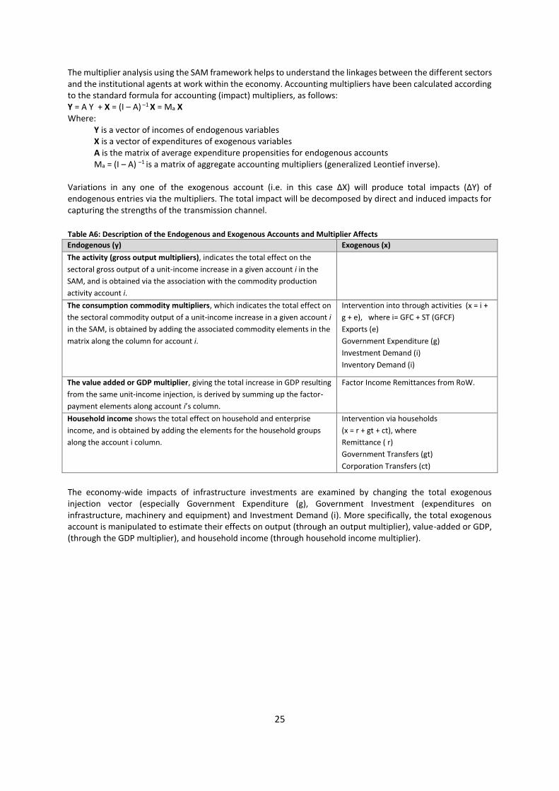
The multiplier analysis using the SAM framework helps to understand the linkages between the different sectors and the institutional agents at work within the economy. Accounting multipliers have been calculated according to the standard formula for accounting (impact) multipliers, as follows: Y = A Y + X = (I – A) –1 X = Ma X Where:

Y is a vector of incomes of endogenous variables X is a vector of expenditures of exogenous variables A is the matrix of average expenditure propensities for endogenous accounts Ma = (I – A) –1 is a matrix of aggregate accounting multipliers (generalized Leontief inverse).

Variations in any one of the exogenous account (i.e. in this case ΔX) will produce total impacts (ΔY) of endogenous entries via the multipliers. The total impact will be decomposed by direct and induced impacts for capturing the strengths of the transmission channel.

Table A6: Description of the Endogenous and Exogenous Accounts and Multiplier Affects

Endogenous (y) Exogenous (x)

The activity (gross output multipliers), indicates the total effect on the

sectoral gross output of a unit-income increase in a given account i in the

SAM, and is obtained via the association with the commodity production

activity account i.

The consumption commodity multipliers, which indicates the total effect on

the sectoral commodity output of a unit-income increase in a given account i

in the SAM, is obtained by adding the associated commodity elements in the

matrix along the column for account i.

Intervention into through activities (x = i +

g + e), where i= GFC + ST (GFCF)

Exports (e)

Government Expenditure (g)

Investment Demand (i)

Inventory Demand (i)

The value added or GDP multiplier, giving the total increase in GDP resulting

from the same unit-income injection, is derived by summing up the factor-

payment elements along account i’s column.

Factor Income Remittances from RoW.

Household income shows the total effect on household and enterprise

income, and is obtained by adding the elements for the household groups

along the account i column.

Intervention via households

(x = r + gt + ct), where

Remittance ( r)

Government Transfers (gt)

Corporation Transfers (ct)

The economy-wide impacts of infrastructure investments are examined by changing the total exogenous injection vector (especially Government Expenditure (g), Government Investment (expenditures on infrastructure, machinery and equipment) and Investment Demand (i). More specifically, the total exogenous account is manipulated to estimate their effects on output (through an output multiplier), value-added or GDP, (through the GDP multiplier), and household income (through household income multiplier).

26

Estimated Economy Wide Benefit

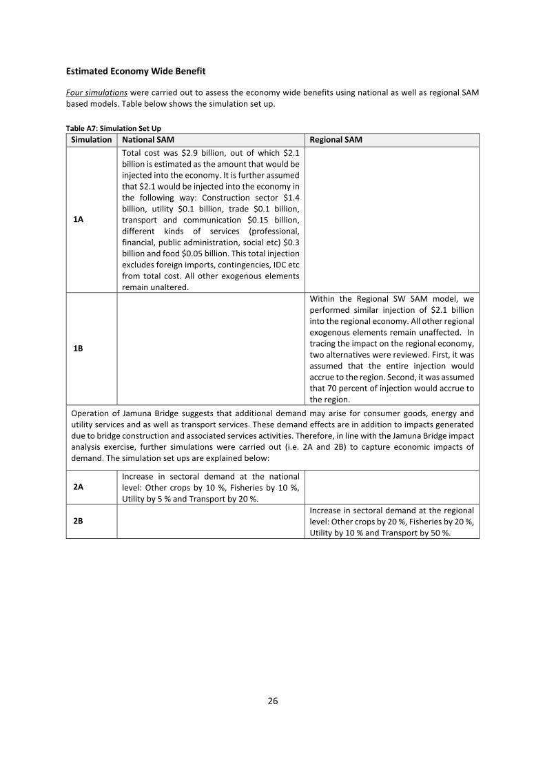
Four simulations were carried out to assess the economy wide benefits using national as well as regional SAM based models. Table below shows the simulation set up.

Table A7: Simulation Set Up

Simulation National SAM Regional SAM

1A

Total cost was $2.9 billion, out of which $2.1 billion is estimated as the amount that would be injected into the economy. It is further assumed that $2.1 would be injected into the economy in the following way: Construction sector $1.4 billion, utility $0.1 billion, trade $0.1 billion, transport and communication $0.15 billion, different kinds of services (professional, financial, public administration, social etc) $0.3 billion and food $0.05 billion. This total injection excludes foreign imports, contingencies, IDC etc from total cost. All other exogenous elements remain unaltered.

1B

Within the Regional SW SAM model, we performed similar injection of $2.1 billion into the regional economy. All other regional exogenous elements remain unaffected. In tracing the impact on the regional economy, two alternatives were reviewed. First, it was assumed that the entire injection would accrue to the region. Second, it was assumed that 70 percent of injection would accrue to the region.

Operation of Jamuna Bridge suggests that additional demand may arise for consumer goods, energy and utility services and as well as transport services. These demand effects are in addition to impacts generated due to bridge construction and associated services activities. Therefore, in line with the Jamuna Bridge impact analysis exercise, further simulations were carried out (i.e. 2A and 2B) to capture economic impacts of demand. The simulation set ups are explained below:

2A Increase in sectoral demand at the national level: Other crops by 10 %, Fisheries by 10 %, Utility by 5 % and Transport by 20 %.

2B Increase in sectoral demand at the regional

level: Other crops by 20 %, Fisheries by 20 %, Utility by 10 % and Transport by 50 %.

27

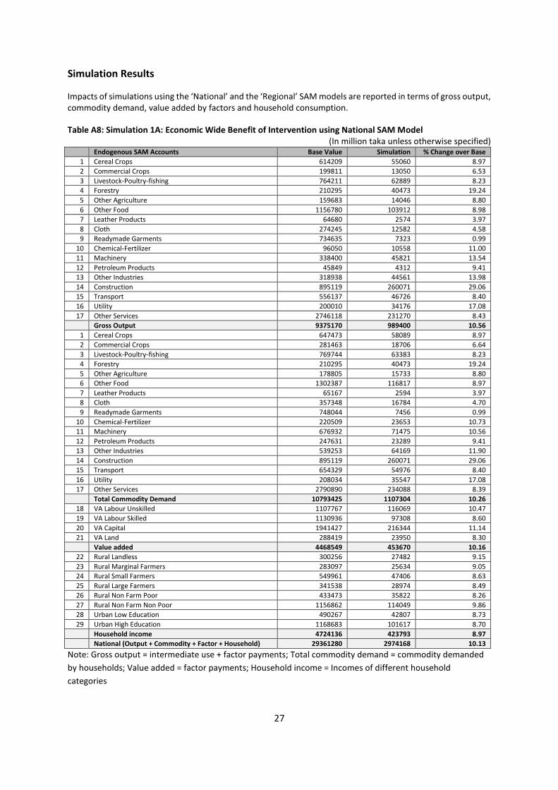
Simulation Results

Impacts of simulations using the ‘National’ and the ‘Regional’ SAM models are reported in terms of gross output, commodity demand, value added by factors and household consumption.

Table A8: Simulation 1A: Economic Wide Benefit of Intervention using National SAM Model (In million taka unless otherwise specified)

Endogenous SAM Accounts Base Value Simulation % Change over Base

1 Cereal Crops 614209 55060 8.97

2 Commercial Crops 199811 13050 6.53

3 Livestock-Poultry-fishing 764211 62889 8.23

4 Forestry 210295 40473 19.24

5 Other Agriculture 159683 14046 8.80

6 Other Food 1156780 103912 8.98

7 Leather Products 64680 2574 3.97

8 Cloth 274245 12582 4.58

9 Readymade Garments 734635 7323 0.99

10 Chemical-Fertilizer 96050 10558 11.00

11 Machinery 338400 45821 13.54

12 Petroleum Products 45849 4312 9.41

13 Other Industries 318938 44561 13.98

14 Construction 895119 260071 29.06

15 Transport 556137 46726 8.40

16 Utility 200010 34176 17.08

17 Other Services 2746118 231270 8.43

Gross Output 9375170 989400 10.56

1 Cereal Crops 647473 58089 8.97



4 Forestry 210295 40473 19.24


6 Other Food 1302387 116817 8.97


8 Cloth 357348 16784 4.70



11 Machinery 676932 71475 10.56



14 Construction 895119 260071 29.06

15 Transport 654329 54976 8.40

16 Utility 208034 35547 17.08

17 Other Services 2790890 234088 8.39

Total Commodity Demand 10793425 1107304 10.26

18 VA Labour Unskilled 1107767 116069 10.47

19 VA Labour Skilled 1130936 97308 8.60

20 VA Capital 1941427 216344 11.14

21 VA Land 288419 23950 8.30

Value added 4468549 453670 10.16

22 Rural Landless 300256 27482 9.15

23 Rural Marginal Farmers 283097 25634 9.05

24 Rural Small Farmers 549961 47406 8.63

25 Rural Large Farmers 341538 28974 8.49

26 Rural Non Farm Poor 433473 35822 8.26

27 Rural Non Farm Non Poor 1156862 114049 9.86

28 Urban Low Education 490267 42807 8.73

29 Urban High Education 1168683 101617 8.70

Household income 4724136 423793 8.97

National (Output + Commodity + Factor + Household) 29361280 2974168 10.13

Note: Gross output = intermediate use + factor payments; Total commodity demand = commodity demanded

by households; Value added = factor payments; Household income = Incomes of different household

categories

28

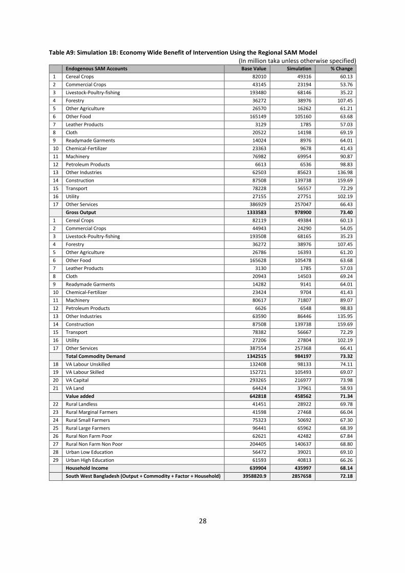
Table A9: Simulation 1B: Economy Wide Benefit of Intervention Using the Regional SAM Model (In million taka unless otherwise specified)

Endogenous SAM Accounts Base Value Simulation % Change

1 Cereal Crops 82010 49316 60.13



4 Forestry 36272 38976 107.45


6 Other Food 165149 105160 63.68


8 Cloth 20522 14198 69.19



11 Machinery 76982 69954 90.87



14 Construction 87508 139738 159.69

15 Transport 78228 56557 72.29

16 Utility 27155 27751 102.19

17 Other Services 386929 257047 66.43

Gross Output 1333583 978900 73.40

1 Cereal Crops 82119 49384 60.13



4 Forestry 36272 38976 107.45


6 Other Food 165628 105478 63.68


8 Cloth 20943 14503 69.24



11 Machinery 80617 71807 89.07



14 Construction 87508 139738 159.69

15 Transport 78382 56667 72.29

16 Utility 27206 27804 102.19

17 Other Services 387554 257368 66.41




20 VA Capital 293265 216977 73.98

21 VA Land 64424 37961 58.93

Value added 642818 458562 71.34

22 Rural Landless 41451 28922 69.78








Household Income 639904 435997 68.14

South West Bangladesh (Output + Commodity + Factor + Household) 3958820.9 2857658 72.18

29

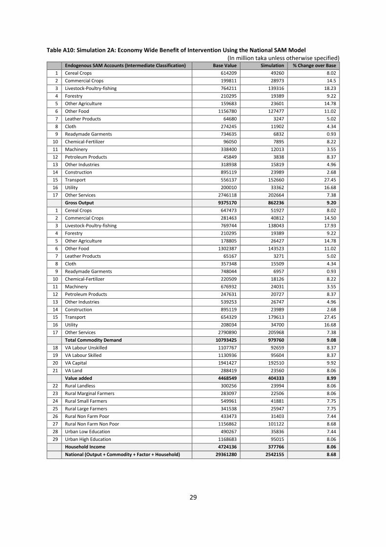
Table A10: Simulation 2A: Economy Wide Benefit of Intervention Using the National SAM Model (In million taka unless otherwise specified)

Endogenous SAM Accounts (Intermediate Classification) Base Value Simulation % Change over Base

1 Cereal Crops 614209 49260 8.02



4 Forestry 210295 19389 9.22


6 Other Food 1156780 127477 11.02


8 Cloth 274245 11902 4.34



11 Machinery 338400 12013 3.55



14 Construction 895119 23989 2.68

15 Transport 556137 152660 27.45

16 Utility 200010 33362 16.68

17 Other Services 2746118 202664 7.38

Gross Output 9375170 862236 9.20

1 Cereal Crops 647473 51927 8.02



4 Forestry 210295 19389 9.22


6 Other Food 1302387 143523 11.02


8 Cloth 357348 15509 4.34



11 Machinery 676932 24031 3.55



14 Construction 895119 23989 2.68

15 Transport 654329 179613 27.45

16 Utility 208034 34700 16.68

17 Other Services 2790890 205968 7.38




20 VA Capital 1941427 192510 9.92

21 VA Land 288419 23560 8.06

Value added 4468549 404333 8.99

22 Rural Landless 300256 23994 8.06









National (Output + Commodity + Factor + Household) 29361280 2542155 8.68

30

Table A11: Simulation 2B: Economy Wide Benefit of Intervention Using the Regional SAM Model (In million taka unless otherwise specified)

Endogenous SAM Accounts (Intermediate Classification) Base Value Simulation % Change over Base

1 Cereal Crops 82010 44117 8.02



4 Forestry 36272 22432 61.84


6 Other Food 165149 122075 73.92


8 Cloth 20522 5974 29.11



11 Machinery 76982 18331 23.81



14 Construction 87508 15731 17.98

15 Transport 78228 144036 184.12

16 Utility 27155 30382 111.88

17 Other Services 386929 191538 49.50

Gross Output 1333583 938825 70.40

1 Cereal Crops 82119 6586 8.02



4 Forestry 36272 22432 61.84


6 Other Food 165628 122429 73.92


8 Cloth 20943 6097 29.11



11 Machinery 80617 19197 23.81



14 Construction 87508 2345 2.68

15 Transport 78382 144320 184.12

16 Utility 27206 30439 111.88

17 Other Services 387554 191848 49.50




20 VA Capital 293265 192510 62

21 VA Land 64424 23560 51.77

Value added 642818 404333 62

22 Rural Landless 41451 23994 60.76









South West Bangladesh (Output + Commodity + Factor + Household) 3958820.9 2542155 61.07

31

Annex 5: Estimated Benefit Cost Ratio Table A12: Estimated BCR @10% Discount Rate (SIM 1)

Cost Project Benefits Net

Year Capital O&M Total Road User Benefits Non Road User Benefits Total Economic

End June Cost Cost VOC TTC Sub-total Ferry Land Utilities WEB Benefits Benefits

2011 60 0 60 0 0 0 0 0 0 0 0 -60

2012 500 0 500 0 0 0 0 0 0 0 0 -500

2013 500 0 500 0 0 0 0 0 0 0 0 -500

2014 500 0 500 0 0 0 0 0 0 0 0 -500

2015 600 0 600 0 0 0 0 0 0 0 0 -600

2016 600 13 613 0 0 0 0 0 0 0 0 -613

2017 600 25 625 0 0 0 0 0 0 0 0 -625

2018 324 25 349 0 0 0 0 0 0 0 0 -349

2019 0 25 25 19 31 50 0 384 271 0 705 680

2020 0 25 25 37 50 87 0 0 0 0 87 62

2021 0 25 25 61 75 136 0 0 0 45.5 181.5 156.5

2022 0 25 25 74 87 161 0 0 0 50 211 186

2023 0 15 15 84 97 181 0 0 0 80 261 246

2024 0 15 15 93 106 199 0 0 0 100 299 284

2025 0 15 15 111 124 235 0 0 0 110 345 330

2026 0 15 15 131 145 276 0 0 0 110 386 371

2027 0 15 15 153 168 321 0 0 0 110 431 416

2028 0 15 15 176 193 369 0 0 0 110 479 464

2029 0 15 15 202 221 423 0 0 0 120 543 528

2030 0 15 15 231 243 474 0 0 0 120 594 579

2031 0 15 15 260 266 526 0 0 0 120 646 631

2032 0 15 15 290 291 581 0 0 0 120 701 686

2033 0 15 15 322 316 638 0 0 0 120 758 743

2034 0 15 15 354 342 696 0 0 0 120 816 801

2035 0 15 15 370 351 721 0 0 0 120 841 826

2036 0 15 15 386 360 746 0 0 0 120 866 851

2037 0 15 15 401 370 771 0 0 0 120 891 876

2038 0 15 15 417 378 795 0 0 0 120 915 900

2039 0 15 15 431 388 819 0 0 0 120 939 924

2040 0 15 15 447 397 844 0 0 0 120 964 949

2041 0 15 15 462 407 869 0 0 0 120 989 974

2042 0 15 15 477 417 894 0 0 0 120 1014 999

2043 0 15 15 493 427 920 0 0 0 120 1040 1025

2044 0 15 15 508 437 945 0 0 0 120 1065 1050

2045 0 15 15 513 438 951 0 0 0 120 1071 1056

2046 0 15 15 518 439 957 0 0 0 120 1077 1062

2047 0 15 15 521 440 961 0 0 0 120 1081 1066

2048 0 15 15 525 441 966 0 0 0 120 1086 1071

2049 0 15 15 542 455 997 0 0 0 120 1117 1102

Total 3684 568 4252 9609 8900 18509 0 384 271 3236 22400

2,415 113 2,528 787 792 1,579 0 163 115 360 2,217

32

Table A13: Estimated BCR @10% Discount Rate (SIM 2)




2011 60 0 60 0 0 0 0 0 0 0 0 -60

2012 500 0 500 0 0 0 0 0 0 0 0 -500

2013 500 0 500 0 0 0 0 0 0 0 0 -500

2014 500 0 500 0 0 0 0 0 0 0 0 -500

2015 600 0 600 0 0 0 0 0 0 0 0 -600

2016 600 13 613 0 0 0 0 0 0 0 0 -613

2017 600 25 625 0 0 0 0 0 0 0 0 -625

2018 324 25 349 0 0 0 0 0 0 0 0 -349

2019 0 25 25 19 31 50 0 384 271 0 705 680

2020 0 25 25 37 50 87 0 0 0 0 87 62

2021 0 25 25 61 75 136 0 0 0 27.3 163.3 138.3

2022 0 25 25 74 87 161 0 0 0 30 191 166

2023 0 15 15 84 97 181 0 0 0 48 229 214

2024 0 15 15 93 106 199 0 0 0 60 259 244

2025 0 15 15 111 124 235 0 0 0 66 301 286

2026 0 15 15 131 145 276 0 0 0 66 342 327

2027 0 15 15 153 168 321 0 0 0 66 387 372

2028 0 15 15 176 193 369 0 0 0 66 435 420

2029 0 15 15 202 221 423 0 0 0 72 495 480

2030 0 15 15 231 243 474 0 0 0 72 546 531

2031 0 15 15 260 266 526 0 0 0 72 598 583

2032 0 15 15 290 291 581 0 0 0 72 653 638

2033 0 15 15 322 316 638 0 0 0 72 710 695

2034 0 15 15 354 342 696 0 0 0 72 768 753

2035 0 15 15 370 351 721 0 0 0 72 793 778

2036 0 15 15 386 360 746 0 0 0 72 818 803

2037 0 15 15 401 370 771 0 0 0 72 843 828

2038 0 15 15 417 378 795 0 0 0 72 867 852

2039 0 15 15 431 388 819 0 0 0 72 891 876

2040 0 15 15 447 397 844 0 0 0 72 916 901

2041 0 15 15 462 407 869 0 0 0 72 941 926

2042 0 15 15 477 417 894 0 0 0 72 966 951

2043 0 15 15 493 427 920 0 0 0 72 992 977

2044 0 15 15 508 437 945 0 0 0 72 1017 1002

2045 0 15 15 513 438 951 0 0 0 72 1023 1008

2046 0 15 15 518 439 957 0 0 0 72 1029 1014

2047 0 15 15 521 440 961 0 0 0 72 1033 1018

2048 0 15 15 525 441 966 0 0 0 72 1038 1023

2049 0 15 15 542 455 997 0 0 0 72 1069 1054

Total 3684 568 4252 9609 8900 18509 0 384 271 1941 21105

2,415 113 2,528 787 792 1,579 0 163 115 216 2,073

33





2011 60 0 60 0 0 0 0 0 0 0 0 -60

2012 500 0 500 0 0 0 0 0 0 0 0 -500

2013 500 0 500 0 0 0 0 0 0 0 0 -500

2014 500 0 500 0 0 0 0 0 0 0 0 -500

2015 600 0 600 0 0 0 0 0 0 0 0 -600

2016 600 13 613 0 0 0 0 0 0 0 0 -613

2017 600 25 625 0 0 0 0 0 0 0 0 -625

2018 324 25 349 0 0 0 0 0 0 0 0 -349

2019 0 25 25 19 31 50 0 384 271 0 705 680

2020 0 25 25 37 50 87 0 0 0 0 87 62

2021 0 25 25 61 75 136 0 0 0 45.5 181.5 156.5

2022 0 25 25 74 87 161 0 0 0 50 211 186

2023 0 15 15 84 97 181 0 0 0 80 261 246

2024 0 15 15 93 106 199 0 0 0 100 299 284

2025 0 15 15 111 124 235 0 0 0 110 345 330

2026 0 15 15 131 145 276 0 0 0 110 386 371

2027 0 15 15 153 168 321 0 0 0 110 431 416

2028 0 15 15 176 193 369 0 0 0 110 479 464

2029 0 15 15 202 221 423 0 0 0 120 543 528

2030 0 15 15 231 243 474 0 0 0 120 594 579

2031 0 15 15 260 266 526 0 0 0 120 646 631

2032 0 15 15 290 291 581 0 0 0 120 701 686

2033 0 15 15 322 316 638 0 0 0 120 758 743

2034 0 15 15 354 342 696 0 0 0 120 816 801

2035 0 15 15 370 351 721 0 0 0 120 841 826

2036 0 15 15 386 360 746 0 0 0 120 866 851

2037 0 15 15 401 370 771 0 0 0 120 891 876

2038 0 15 15 417 378 795 0 0 0 120 915 900

2039 0 15 15 431 388 819 0 0 0 120 939 924

2040 0 15 15 447 397 844 0 0 0 120 964 949

2041 0 15 15 462 407 869 0 0 0 120 989 974

2042 0 15 15 477 417 894 0 0 0 120 1014 999

2043 0 15 15 493 427 920 0 0 0 120 1040 1025

2044 0 15 15 508 437 945 0 0 0 120 1065 1050

2045 0 15 15 513 438 951 0 0 0 120 1071 1056

2046 0 15 15 518 439 957 0 0 0 120 1077 1062

2047 0 15 15 521 440 961 0 0 0 120 1081 1066

2048 0 15 15 525 441 966 0 0 0 120 1086 1071

2049 0 15 15 542 455 997 0 0 0 120 1117 1102

Total 3684 568 4252 9609 8900 18509 0 384 271 3236 22400

2,977 227 3,204 2,499 2,407 4,906 0 248 175 984 6,312

34





2011 60 0 60 0 0 0 0 0 0 0 0 -60

2012 500 0 500 0 0 0 0 0 0 0 0 -500

2013 500 0 500 0 0 0 0 0 0 0 0 -500

2014 500 0 500 0 0 0 0 0 0 0 0 -500

2015 600 0 600 0 0 0 0 0 0 0 0 -600

2016 600 13 613 0 0 0 0 0 0 0 0 -613

2017 600 25 625 0 0 0 0 0 0 0 0 -625

2018 324 25 349 0 0 0 0 0 0 0 0 -349

2019 0 25 25 19 31 50 0 384 271 0 705 680

2020 0 25 25 37 50 87 0 0 0 0 87 62

2021 0 25 25 61 75 136 0 0 0 27.3 163.3 138.3

2022 0 25 25 74 87 161 0 0 0 30 191 166

2023 0 15 15 84 97 181 0 0 0 48 229 214

2024 0 15 15 93 106 199 0 0 0 60 259 244

2025 0 15 15 111 124 235 0 0 0 66 301 286

2026 0 15 15 131 145 276 0 0 0 66 342 327

2027 0 15 15 153 168 321 0 0 0 66 387 372

2028 0 15 15 176 193 369 0 0 0 66 435 420

2029 0 15 15 202 221 423 0 0 0 72 495 480

2030 0 15 15 231 243 474 0 0 0 72 546 531

2031 0 15 15 260 266 526 0 0 0 72 598 583

2032 0 15 15 290 291 581 0 0 0 72 653 638

2033 0 15 15 322 316 638 0 0 0 72 710 695

2034 0 15 15 354 342 696 0 0 0 72 768 753

2035 0 15 15 370 351 721 0 0 0 72 793 778

2036 0 15 15 386 360 746 0 0 0 72 818 803

2037 0 15 15 401 370 771 0 0 0 72 843 828

2038 0 15 15 417 378 795 0 0 0 72 867 852

2039 0 15 15 431 388 819 0 0 0 72 891 876

2040 0 15 15 447 397 844 0 0 0 72 916 901

2041 0 15 15 462 407 869 0 0 0 72 941 926

2042 0 15 15 477 417 894 0 0 0 72 966 951

2043 0 15 15 493 427 920 0 0 0 72 992 977

2044 0 15 15 508 437 945 0 0 0 72 1017 1002

2045 0 15 15 513 438 951 0 0 0 72 1023 1008

2046 0 15 15 518 439 957 0 0 0 72 1029 1014

2047 0 15 15 521 440 961 0 0 0 72 1033 1018

2048 0 15 15 525 441 966 0 0 0 72 1038 1023

2049 0 15 15 542 455 997 0 0 0 72 1069 1054

Total 3684 568 4252 9609 8900 18509 0 384 271 1941 21105

2,977 227 3,204 2,499 2,407 4,906 0 248 175 590 5,918

35

Table A16: Estimated BCR @ 3% Discount Rate (SIM 1)


Year Capital

O&M

Total Road User Benefits Non Road User Benefits Total Economic

End June Cost Cost VOC TTC Sub-total

Ferry

Land

Utilities

WEB Benefits

Benefits

2011 60 0 60 0 0 0 0 0 0 0 0 -60

2012 500 0 500 0 0 0 0 0 0 0 0 -500

2013 500 0 500 0 0 0 0 0 0 0 0 -500

2014 500 0 500 0 0 0 0 0 0 0 0 -500

2015 600 0 600 0 0 0 0 0 0 0 0 -600

2016 600 13 613 0 0 0 0 0 0 0 0 -613

2017 600 25 625 0 0 0 0 0 0 0 0 -625

2018 324 25 349 0 0 0 0 0 0 0 0 -349

2019 0 25 25 19 31 50 0 384 271 0 705 680

2020 0 25 25 37 50 87 0 0 0 0 87 62

2021 0 25 25 61 75 136 0 0 0 45.5 181.5 156.5

2022 0 25 25 74 87 161 0 0 0 50 211 186

2023 0 15 15 84 97 181 0 0 0 80 261 246

2024 0 15 15 93 106 199 0 0 0 100 299 284

2025 0 15 15 111 124 235 0 0 0 110 345 330

2026 0 15 15 131 145 276 0 0 0 110 386 371

2027 0 15 15 153 168 321 0 0 0 110 431 416

2028 0 15 15 176 193 369 0 0 0 110 479 464

2029 0 15 15 202 221 423 0 0 0 120 543 528

2030 0 15 15 231 243 474 0 0 0 120 594 579

2031 0 15 15 260 266 526 0 0 0 120 646 631

2032 0 15 15 290 291 581 0 0 0 120 701 686

2033 0 15 15 322 316 638 0 0 0 120 758 743

2034 0 15 15 354 342 696 0 0 0 120 816 801

2035 0 15 15 370 351 721 0 0 0 120 841 826

2036 0 15 15 386 360 746 0 0 0 120 866 851

2037 0 15 15 401 370 771 0 0 0 120 891 876

2038 0 15 15 417 378 795 0 0 0 120 915 900

2039 0 15 15 431 388 819 0 0 0 120 939 924

2040 0 15 15 447 397 844 0 0 0 120 964 949

2041 0 15 15 462 407 869 0 0 0 120 989 974

2042 0 15 15 477 417 894 0 0 0 120 1014 999

2043 0 15 15 493 427 920 0 0 0 120 1040 1025

2044 0 15 15 508 437 945 0 0 0 120 1065 1050

2045 0 15 15 513 438 951 0 0 0 120 1071 1056

2046 0 15 15 518 439 957 0 0 0 120 1077 1062

2047 0 15 15 521 440 961 0 0 0 120 1081 1066

2048 0 15 15 525 441 966 0 0 0 120 1086 1071

2049 0 15 15 542 455 997 0 0 0 120 1117 1102

Total 3684 568 4252 9609 8900 18509 0 384 271 3236 22400

3,255 317 3,57

2 4,182 3,963 8,145 0 294 208

1,54

5 10,192

36

Table A17: Estimated BCR @ 3% Discount Rate (SIM 2)




2011 60 0 60 0 0 0 0 0 0 0 0 -60

2012 500 0 500 0 0 0 0 0 0 0 0 -500

2013 500 0 500 0 0 0 0 0 0 0 0 -500

2014 500 0 500 0 0 0 0 0 0 0 0 -500

2015 600 0 600 0 0 0 0 0 0 0 0 -600

2016 600 13 613 0 0 0 0 0 0 0 0 -613

2017 600 25 625 0 0 0 0 0 0 0 0 -625

2018 324 25 349 0 0 0 0 0 0 0 0 -349

2019 0 25 25 19 31 50 0 384 271 0 705 680

2020 0 25 25 37 50 87 0 0 0 0 87 62

2021 0 25 25 61 75 136 0 0 0 27.3 163.3 138.3

2022 0 25 25 74 87 161 0 0 0 30 191 166

2023 0 15 15 84 97 181 0 0 0 48 229 214

2024 0 15 15 93 106 199 0 0 0 60 259 244

2025 0 15 15 111 124 235 0 0 0 66 301 286

2026 0 15 15 131 145 276 0 0 0 66 342 327

2027 0 15 15 153 168 321 0 0 0 66 387 372

2028 0 15 15 176 193 369 0 0 0 66 435 420

2029 0 15 15 202 221 423 0 0 0 72 495 480

2030 0 15 15 231 243 474 0 0 0 72 546 531

2031 0 15 15 260 266 526 0 0 0 72 598 583

2032 0 15 15 290 291 581 0 0 0 72 653 638

2033 0 15 15 322 316 638 0 0 0 72 710 695

2034 0 15 15 354 342 696 0 0 0 72 768 753

2035 0 15 15 370 351 721 0 0 0 72 793 778

2036 0 15 15 386 360 746 0 0 0 72 818 803

2037 0 15 15 401 370 771 0 0 0 72 843 828

2038 0 15 15 417 378 795 0 0 0 72 867 852

2039 0 15 15 431 388 819 0 0 0 72 891 876

2040 0 15 15 447 397 844 0 0 0 72 916 901

2041 0 15 15 462 407 869 0 0 0 72 941 926

2042 0 15 15 477 417 894 0 0 0 72 966 951

2043 0 15 15 493 427 920 0 0 0 72 992 977

2044 0 15 15 508 437 945 0 0 0 72 1017 1002

2045 0 15 15 513 438 951 0 0 0 72 1023 1008

2046 0 15 15 518 439 957 0 0 0 72 1029 1014

2047 0 15 15 521 440 961 0 0 0 72 1033 1018

2048 0 15 15 525 441 966 0 0 0 72 1038 1023

2049 0 15 15 542 455 997 0 0 0 72 1069 1054

Total 3684 568 4252 9609 8900 18509 0 384 271 1941 21105

3,255 317 3,572 4,182 3,963 8,145 0 294 208 927 9,574

© Copenhagen Consensus Center 2016

Bangladesh, like most nations, faces a large number of challenges. What should be the top priorities for policy makers, international donors, NGOs and businesses? With limited resources and time, it is crucial that focus is informed by what will do the most good for each taka spent. The Bangladesh Priorities project, a collaboration between Copenhagen Consensus and BRAC, works with stakeholders across Bangladesh to find, analyze, rank and disseminate the best solutions for the country. We engage Bangladeshis from all parts of society, through readers of newspapers, along with NGOs, decision makers, sector experts and businesses to propose the best solutions. We have commissioned some of the best economists from Bangladesh and the world to calculate the social, environmental and economic costs and benefits of these proposals. This research will help set priorities for the country through a nationwide conversation about what the smart - and not-so-smart - solutions are for Bangladesh's future.

For more information vis it w ww .Bangladesh -Prior it ies.com

C O P E N H A G E N C O N S E N S U S C E N T E R Copenhagen Consensus Center is a think tank that investigates and publishes the best policies and investment opportunities based on social good (measured in dollars, but also incorporating e.g. welfare, health and environmental protection) for every dollar spent. The Copenhagen Consensus was conceived to address a fundamental, but overlooked topic in international development: In a world with limited budgets and attention spans, we need to find effective ways to do the most good for the most people. The Copenhagen Consensus works with 300+ of the world's top economists including 7 Nobel Laureates to prioritize solutions to the world's biggest problems, on the basis of data and cost-benefit analysis.

Documents

Economic Cost-Benefit Analysis: Padma Bridge Project · Economic Cost-Benefit Analysis: Padma Bridge Project Bangladesh Priorities Ashikur Rahman Senior Economist, Policy Research