Embed Size (px)
Citation preview
www.elsevier.com/locate/econbase
Journal of International Economics 62 (2004) 53–82
Economic geography and international inequality
Stephen Redding*, Anthony J. Venables1
Department of Economics, LSE Houghton Street London WC2A 2AE, UK
Received 25 April 2002; received in revised form 8 July 2003; accepted 14 July 2003
Abstract
This paper estimates a structural model of economic geography using cross-country data on per
capita income, bilateral trade, and the relative price of manufacturing goods. We provide evidence
that the geography of access to markets and sources of supply is statistically significant and
quantitatively important in explaining cross-country variation in per capita income. This finding is
robust to controlling for a wide range of considerations, including other economic, geographical,
social, and institutional characteristics. Geography is found to matter through the mechanisms
emphasized by the theory, and the estimated coefficients are consistent with plausible values for the
model’s structural parameters.
D 2003 Elsevier B.V. All rights reserved.
Keywords: Economic development; Economic geography; International trade
JEL classification: F12; F14; O10
1. Introduction
In 1996, manufacturing wages at the 90th percentile of the cross-country distribution
were more than 50 times higher than those at the 10th percentile. Despite increasing
international economic integration, these vast disparities in wages have not been bid away
by the mobility of manufacturing firms and plants. There are many potential reasons for
the reluctance of firms to move production to low wage countries, including endowments,
technology, institutional quality, and geographical location. This paper focuses on the role
of geographical location. We estimate its effects using a fully specified model of economic
0022-1996/$ - see front matter D 2003 Elsevier B.V. All rights reserved.
doi:10.1016/j.jinteco.2003.07.001
* Corresponding author. Tel.: +44-20-7955-7483; fax: +44-20-7831-1840.
E-mail addresses: [email protected] (S. Redding), [email protected] (A.J. Venables).
URLs: http://econ.lse.ac.uk/~sredding/, http://econ.lse.ac.uk/staff/ajv.1 Tel.: +44-20-7955-7522; fax: +44-20-7831-1840.
S. Redding, A.J. Venables / Journal of International Economics 62 (2004) 53–8254
geography (that of Fujita et al., 1999) and cross-country data including per capita income,
bilateral trade, and the relative price of manufacturing goods.
Geographical location may affect per capita income in a number of ways, through its
influence on flows of goods, factors of production, and ideas. In this paper, we concentrate
on two mechanisms. One is the distance of countries from the markets in which they sell
output, and the other is distance from countries that supply manufactures and provide the
capital equipment and intermediate goods required for production. Transport costs or other
barriers to trade mean that more distant countries suffer a market access penalty on their
sales and also face additional costs on imported inputs. As a consequence, firms in these
countries can only afford to pay relatively low wages—even if, for example, their
technologies are the same as those elsewhere.
The potential impact of these effects is easily illustrated. Suppose that the prices of
output and intermediate goods are set on world markets, transport costs are borne by the
producing country, and intermediates account for 50% of costs. Ad valorem transport costs
of 10% on both final output and intermediate goods have the effect of reducing domestic
value added by 30% (compared to a country facing zero transport costs), the reduction in
value added rising to 60% for transport costs of 20%, and to 90% for transport costs of
30%.2 Transport costs of this magnitude are consistent with recent empirical evidence. For
example, using customs data, Hummels (1999) finds that average expenditure on freight
and insurance as a proportion of the value of manufacturing imports is 10.3% in US,
15.5% in Argentina, and 17.7% in Brazil. Limao and Venables (2001) relate transport costs
to features of economic geography finding, for example, that the median land-locked
country’s shipping costs are more than 50% higher than those of the median coastal
country. Each of these papers focuses on transport costs narrowly defined (pure costs of
freight and insurance) and may understate the true magnitude of barriers to trade if there
are other costs to transacting at a distance, such as costs of information acquisition and of
time in transit.
Our model formalizes the role of economic geography in determining equilibrium
factor prices, and the exact specifications suggested by theory are used to estimate the
magnitude of these effects. When included by itself, the geography of access to markets
and sources of supply can explain much of the cross-country variation in per capita
income. After controlling for a variety of other determinants of per capita income, we
continue to find highly statistically significant and quantitatively important effects of
economic geography.
The methodology we employ is as follows. We develop a theoretical trade and
geography model to derive three relationships for empirical study. The first of these is
a gravity-like relationship for bilateral trade flows between countries. Estimation of this
enables us to derive economically meaningful estimates of each country’s proximity to
markets and suppliers—measures that we call market access and supplier access,
respectively. Market access is essentially a measure of market potential, measuring
the export demand each country faces given its geographical position and that of its
trading partners; ‘supplier access’ is the analogous measure on the import side, so is an
2 See also Radelet and Sachs (1998).
S. Redding, A.J. Venables / Journal of International Economics 62 (2004) 53–82 55
appropriately distance weighted measure of the location of import supply to each
country. The second relationship is a zero profit condition for firms that implicitly
defines the maximum level of factor prices a representative firm in each country can
afford to pay, given its market access and supplier access. We call this the wage
equation and use it to estimate the relationship between actual income levels and those
predicted by each country’s market access and supplier access. The third relationship is
a price index, suggesting how the prices of manufactures should vary with supplier
access; we also estimate this as a check on one of the key mechanisms in our
approach.
Throughout the paper, we remain very close to the theoretical structure of the trade and
geography model. We find that our market access and supplier access measures are
important determinants of income, and that the estimated coefficients are consistent with
plausible values for the structural parameters of the model. The effects of individual
economic and geographical characteristics are shown to be quantitatively important. For
example, access to the coast and open-trade policies yield predicted increases in per capita
income of over 20%, while halving a country’s distance from all of its trade partners yields
an increase of around 25%. The results are robust to the inclusion of a wide range of
control variables, including countries’ resource endowments, other characteristics of
physical geography (as used by Gallup et al., 1998), and additional institutional, social,
and political controls (see, for example, Hall and Jones, 1999; Knack and Keefer, 1997;
Acemoglu et al., 2001). We also establish the robustness of the results to instrumenting our
market and supplier access measures with exogenous geographical determinants and
provide evidence that economic geography matters for per capita income through the
mechanisms emphasized by the theory.
The idea that access to markets is important for factor incomes dates back at least to
Harris (1954), who argued that the potential demand for goods and services produced
in any one location depends upon the distance-weighted GDP of all locations. Early
econometric investigations of the relationship between market access and per capita
income include Hummels (1995) and Leamer (1997). Hummels (1995) finds that the
residuals from the augmented Solow–Swan neoclassical model of growth are highly
correlated with three alternative measures of geographical location. Leamer (1997)
extends traditional market access measures to improve their treatment of the domestic
market and exploit information on the distance coefficient from a gravity model. He
finds that Central and Eastern European countries’ differing access to Western
European markets creates differences in their potential to achieve higher standards of
living.
Gallup et al. (1998) and Radelet and Sachs (1998) find that measures of physical
geography (e.g., fraction of land area in the geographical tropics) and transport costs
(e.g., percentage of land area within 100 km of the coast or navigable rivers) are
important for cross-country income. Though the focus is not on market access per se,
Frankel and Romer (1999) use geography measures as instruments for trade flows. They
find evidence of a positive relationship between per capita income and exogenous
variation in the ratio of trade to GDP due to the geography measures. This is different
from our approach both conceptually and empirically. For example, the correlation
coefficients between the trade/GDP ratio and our preferred measures of market and
S. Redding, A.J. Venables / Journal of International Economics 62 (2004) 53–8256
supplier access are 0.14 and 0.37, respectively.3 Our work complements the analysis of
market access and wages for US counties by Hanson (1998). It differs from his work in
geographical focus (on countries rather than regions), the use of trade data to reveal
both observed and unobserved determinants of market access, the introduction of
supplier as well as market access, and in having labour immobile between geographical
units.4
The paper is structured as follows. In the next section, we set out the theoretical
model and derive the three structural equations that form the basis of the econometric
estimation. Section 3 discusses the empirical implementation of the model. Sections 4
and 5 present our baseline estimates of the trade equation and the wage equation,
respectively. Section 5 also undertakes a number of robustness tests. Section 6 exploits
the structure of the theoretical model to relate the estimated coefficients to values of the
structural parameters, and Section 7 shows how our approach can be used to disentangle
the effects of a variety of features of economic geography for per capita income. Section
8 concludes.
2. Theoretical framework
The theoretical framework is based on a standard new trade theory model, extended
to have transport frictions in trade and intermediate goods in production.5 The world
consists of i = 1,. . ., R countries, and we focus on the manufacturing sector, composed
of firms that operate under increasing returns to scale and produce differentiated
products.
On the demand side, each firm’s product is differentiated from that of other firms and is
used both in consumption and as an intermediate good. In both uses, there is a constant
elasticity of substitution, r, between pairs of products, so products enter both utility and
production through a CES aggregator taking the form
Uj ¼XRi
Zni
xijðzÞðr�1Þ=rdz
" #r=ðr�1Þ
¼XRi
nixðr�1Þ=rij
" #r=ðr�1Þ
; r > 1; ð1Þ
where z denotes manufacturing varieties, ni is the set of varieties produced in country i,
and xij(z) is the country j demand for the zth product from this set. The second equation
makes use of the fact that, in equilibrium, all products produced in each country i are
demanded by country j in the same quantity, so we dispense with the index z and rewrite
3 We also present empirical results linking factor prices to foreign market and supplier access. The correlation
coefficients between the trade share and our measures of foreign market and supplier access are 0.20 and 0.24,
respectively.4 See Combes and Lafourcade (2001) for an analysis of reductions in transport costs and regional inequalities
within France, and Overman et al. (2003) for a review of the empirical geography literature.5 The exposition follows Fujita et al. (1999), Chapter 14. The full general equilibrium model consists of an
agricultural and manufacturing sector. Manufacturing can be interpreted as a composite of manufacturing and
service activities.
S. Redding, A.J. Venables / Journal of International Economics 62 (2004) 53–82 57
the integral as a product. Dual to this quantity aggregator is a price index for manufactures
in each country, Gj, defined over the prices of individual varieties produced in i and sold in
j, pij,
Gj ¼XRi
Zni
pijðzÞ1�rdz
" #1=1�r
¼XRi
nip1�rij
" #1=1�r
ð2Þ
where the second equation makes use of the symmetry in equilibrium prices.
Country j’s total expenditure on manufactures we denote Ej. Given this expenditure,
country j’s demand for each product is (by Shephard’s lemma on the price index)
xij ¼ p�rij EjG
ðr�1Þj : ð3Þ
Thus, the own price elasticity of demand is r, and the term and EjGj(r � 1), gives the
position of the demand curve facing each firm in market j. We shall refer to this as
the ‘market capacity’ of country j; it depends on total expenditure in j and on the
number of competing firms and the prices they charge, this summarised in the price
index, Gj.
Turning to supply, each representative country i firm has profits pi,
pi ¼XRj
pijxij=Tij � Gai w
bi v
ci ci½F þ xi�: ð4Þ
The final term is costs. The total output of each firm is xiuP
j xij, and technology has
increasing returns to scale, represented by a fixed input requirement ciF and marginal
input requirement ci, these technology parameters potentially varying across countries.
There are three types of inputs, combined in a Cobb–Douglas technology. One is an
internationally immobile composite primary factor which we interpret as labour, with
price wi and input share b. The second is an internationally mobile primary factor with
price vi and input share c. The third is a composite intermediate good with price Gi
and input share a, and we assume a + b + c = 1. The first term in Eq. (4) is revenue
earned from sales in all markets. Tij is an iceberg transport cost factor, so if Tij = 1,
then trade is costless, while Tij� 1 measures the proportion of output lost in shipping
from i to j.
With demand function Eq. (3), profit-maximising firms set a single f.o.b. price, pi, so
prices for sale in different countries are pij = piTij. The price, pi, is a constant markup over
marginal cost, given by
pi ¼ Gai w
bi v
ci cir=ðr � 1Þ: ð5Þ
Given this pricing behaviour, profits of each country i firm are
pi ¼ ðpi=rÞ t xi � ðr � 1ÞF b: ð6Þ
S. Redding, A.J. Venables / Journal of International Economics 62 (2004) 53–8258
Thus, firms break even if the total volume of their sales equals a constant denoted
xu (r� 1)F. From the demand function, Eq. (3), they will sell this many units if price
satisfies6
pri x ¼
XRj
EjGr�1j ðTijÞ1�r: ð7Þ
Substituting the profit maximising price, Eq. (5), firms break even if
xðGai w
bi v
ci cir=ðr � 1ÞÞr ¼
XRj
EjGr�1j T1�r
ij : ð8Þ
We follow Fujita et al. (1999) in calling this the wage equation, although more accurately,
it is an equation for the price of the composite immobile factor of production. This
relationship plays a central role in the empirical analysis below. It says that the maximum
value of the wage that each firm in country i can afford to pay is a function of the sum of
distance weighted market capacities. This sum we will refer to as the ‘market access’ of
country i.
The second relationship we use in the empirical analysis is that defining bilateral trade
flows between countries. The demand Eq. (3) gives the volume of sales per firm to each
location, and expressing these in aggregate value gives exports from i to j of
nipixij ¼ nip1�ri ðTijÞ1�r
EjGr�1j : ð9Þ
The right-hand side of this equation contains both demand and supply variables. The term
EjGjr � 1 is country jmarket capacity, as defined above. On the supply side, the term ni pi
1� r
measures the ‘supply capacity’ of the exporting country; it is the product of the number of
firms and their price competitiveness, such that doubling supply capacity (given market
capacities) doubles the value of sales. In addition, the term (Tij)1� r measures bilateral
transport costs between countries.
The price index forms the third main relationship used in the empirical analysis to
follow. This is already defined in Eq. (2), and given our assumption about transportation
costs, it becomes
Gj ¼Xi
niðpiTijÞ1�r
" #1=ð1�rÞ
: ð10Þ
Notice that the term in square brackets is a sum of supply capacities, weighted by transport
costs, so measures what we shall term the ‘supplier access’ of country j. It is important
because an increase in this supplier access reduces the price index and the cost of
intermediate goods and therefore reduces the costs of production in country j (Eq. (8)).
6 The transport cost term enters with exponent 1�r not � r, because total shipments to market i are Tijtimes quantities consumed.
S. Redding, A.J. Venables / Journal of International Economics 62 (2004) 53–82 59
Supplier access thus summarises the benefit of proximity to suppliers of intermediate
goods.
The full general equilibrium of the model is explored in Fujita et al. (1999) and
involves specifying factor endowments and hence factor market clearing to determine
income and expenditure (Ei), the output levels of each country’s manufacturing (the values
of ni), output in other sectors (primary and non-tradable), and payments balance. Here we
take Ei and ni as exogenous and simply ask, given the locations of expenditure and of
production, what wages can manufacturing firms in each location afford to pay?
3. Empirical framework
The empirical analysis proceeds in several stages. First, we estimate the trade equation
(Eq. (9)) in order to obtain empirical estimates of bilateral transport costs between
countries and of each country’s market and supply capacities. Labelling these mi and si,
respectively, they are defined as
miuEiGr�1i ; siunip
1�ri ; ð11Þ
and allow the trade equation (Eq. (9)) to be rewritten as
nipixij ¼ siðTijÞ1�rmj: ð12Þ
We estimate this gravity-type relationship on bilateral trade flow data, and from it, we
obtain predictions for (Tij)1� rmj and si(Tij)
1� r for each exporting country i and importing
partner j.
Second, we construct the market access of each exporting country i, MAi, and the
supplier access of each importing country j, SAj. Market access is the appropriately
distance-weighted sum of the market capacities of all partner countries, and supplier access
is the analogous sum of supplier capacities, so
MAi ¼Xj
EjGr�1j T1�r
ij ¼Xj
ðTijÞ1�rmj;
SAj ¼Xi
niðpiTijÞ1�r ¼Xi
siðTijÞ1�r: ð13Þ
Using predicted values of (Tij)1� rmj and si(Tij)
1� r from the trade equation, we construct
empirical predictions for these two variables.
Third, using Eqs. (8), (10), (11), and (13), the wage equation for country i can be
written as a log-linear function of its supplier access and market access,
ðwbi v
ci ciÞ
r ¼ AG�ari
XRj
EjGr�1j T1�r
ij ¼ AXj
sjðTijÞ1�r
" # arr�1 X
j
ðTijÞ1�rmj
" #
¼ AðSAiÞar
r�1ðMAiÞ ð14Þ
S. Redding, A.J. Venables / Journal of International Economics 62 (2004) 53–8260
where the left-hand side of Eq. (14) contains the wage, wi, the price of the
internationally mobile factor of production, vi, and a measure of technology differences,
ci; the constant A on the right-hand side combines constants from Eq. (8). The equation
says that countries with high market access and high supplier access pay relatively high
wages. We estimate this equation using predicted values of supplier access and market
access as right-hand side variables, and cross-country data on factor incomes as the
dependent variable. This estimation establishes the extent to which observed variation in
factor incomes can be explained by these geographical determinants, and the estimated
coefficients on these variables can be clearly related to the values of the structural
parameters of the model.
Finally, from Eqs. (10) and (13), the price index for manufacturing goods, Gj, may be
written as a function of supplier access, SAj,
Gj ¼ ½SAj�1=ð1�rÞ: ð15Þ
We estimate Eq. (15) using predicted values of supplier access as the right-hand
side variable and data on the relative price of manufacturing goods on the left-hand
side.
4. Trade equation estimation
4.1. Data sources and sample size
Data on bilateral trade flows for a cross-section of 101 countries are obtained from
the World Bank’s COMTRADE database. We combine the trade data with information
on geographical characteristics (e.g., bilateral distance, existence of a common border)
and data on GDP and population from the World Bank. See Appendix A for further
details.
4.2. Econometric estimation
The value of bilateral trade flows in the trade equation, Eq. (12), depends upon
exporting country characteristics (supply capacity, si), importing partner characteristics
(market capacity, mj), and bilateral transportation costs (Tij). In the main econometric
specification, these exporting and importing country characteristics (supply and market
capacity) are captured with country and partner dummies (denoted by ctyi and ptnj,
respectively). The use of dummies addresses the fact that we cannot observe economic
variables that correspond exactly to the theory and also controls for any component of
transport costs or trade policy that is common across all partners for a particular
exporting country or common across all suppliers of an importing country. Section 7
of the paper repeats the analysis using economic and geographical measures of supply
and market capacity and shows that the main results of the paper are robust to either
approach. The bilateral component of transportation costs is modelled using data on
S. Redding, A.J. Venables / Journal of International Economics 62 (2004) 53–82 61
the distance between capital cities (distij) and a dummy for whether an exporting
country and importing partner share a common border (bordij). Eq. (12) thus becomes7
lnðXijÞ ¼ h þ lictyi þ kjptnj þ d1lnðdistijÞ þ d2bordij þ uij ð16Þ
where Xij denotes the value of exports from country i to partner j, and uij is a
stochastic error. There are a number of observations of zero bilateral trade flows and,
throughout the following, we add 1 to all trade flows before taking logarithms.8
Column (1) of Table 1 presents the results of estimating Eq. (16) on 1994 data using
OLS. The distance between capital cities and common border variables are correctly
signed according to economic priors and statistically significant at the 1% level. The null
hypothesis that the coefficients on either the country dummies or the partner dummies are
equal to zero is easily rejected at the 1% level with a standard F-test, and the model
explains approximately 80% of the cross-section variation in bilateral trade flows.
However, the specification in column (1) does not take into account the fact that the
trade data is left-censored at zero. In column (2), we reestimate the model for the censored
sample using OLS. Column (3) explicitly takes into account the truncated nature of the
data by using the Tobit estimator. This increases the absolute magnitude of the coefficient
on the distance variable and reduces the size of the coefficient on the common border
dummy. We use the Tobit estimates as the basis for our next step.
4.3. Construction of market and supplier access
The coefficients of the country and partner dummies in the trade equation (Eq. (16))
provide estimates of the market and supply capacities of each country, mj and si, capturing
all factors that determine countries’ propensities to demand imports from or supply exports
to all partners. The distance and border coefficients provide estimates of the bilateral
transport cost measure, (Tij)1� r. These give the weights that combine market capacities in
the construction of market access and combine supply capacities in the construction of
supplier access (see Eq. (13)) and are the basis for the spatial variation of market access and
supplier access.9 Predicted values of market access and supplier access are therefore, from
Eq. (13),
MAi ¼ ˆDMAi þ ˆFMAi ¼ ðexpðptniÞÞkiðTiiÞ1�r þ
Xjp i
ðexpðptnjÞÞkjdistd1ij bord
d2ij ð17Þ
SAj ¼ ˆDSAj þ ˆFSAj ¼ ðexpðctyjÞÞljðTjjÞ1�r þ
Xip j
ðexpðctyiÞÞlidistd1ij bord
d2ij ð18Þ
ˆ
ˆ
7 This specification is more general than the standard gravity model, in which country and partner dummies are
replaced by income and other country characteristics. The partner dummies capture the manufacturing price index,
Gj, and thus control for the effects of what Anderson and van Wincoop (2003) term ‘multilateral resistance.’8 The COMTRADE database records the values of bilateral trade flows to a high degree of accuracy; these
zeros are genuine zeros rather than missing values. The trade data are in thousands of dollars, and thus, we add
$1000 before taking logarithms.9 If Tij = 1 for all i, j, then all countries have the same market and supplier access (Eq. (13)).
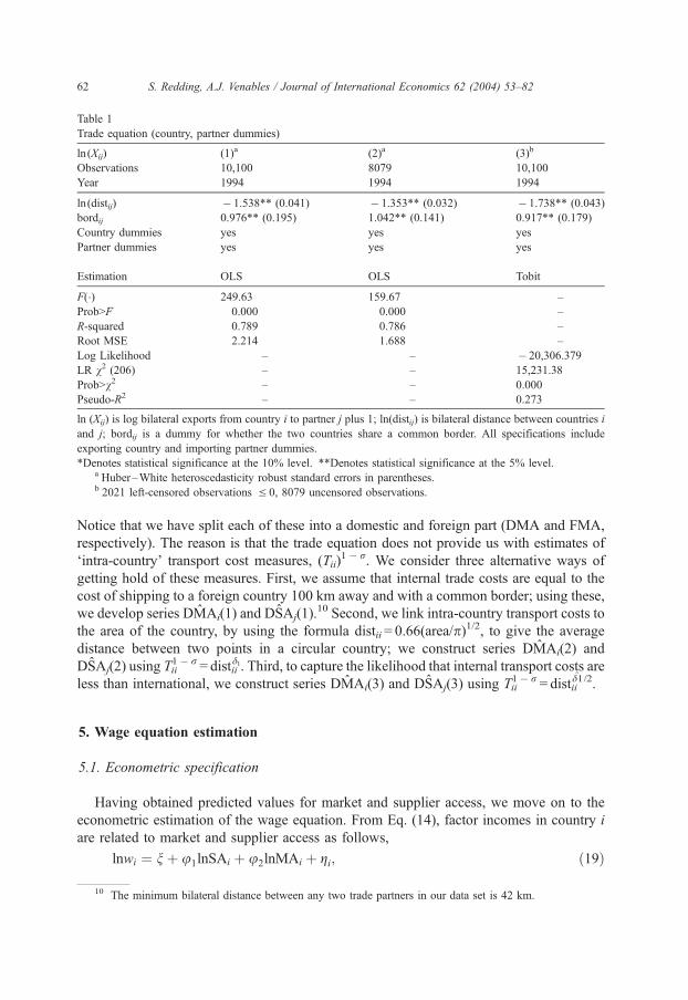
Table 1
Trade equation (country, partner dummies)
ln(Xij) (1)a (2)a (3)b
Observations 10,100 8079 10,100
Year 1994 1994 1994
ln(distij) � 1.538** (0.041) � 1.353** (0.032) � 1.738** (0.043)
bordij 0.976** (0.195) 1.042** (0.141) 0.917** (0.179)
Country dummies yes yes yes
Partner dummies yes yes yes
Estimation OLS OLS Tobit
F(�) 249.63 159.67 –
Prob>F 0.000 0.000 –
R-squared 0.789 0.786 –
Root MSE 2.214 1.688 –
Log Likelihood – – � 20,306.379
LR v2 (206) – – 15,231.38
Prob>v2 – – 0.000
Pseudo-R2 – – 0.273
ln (Xij) is log bilateral exports from country i to partner j plus 1; ln(distij) is bilateral distance between countries i
and j; bordij is a dummy for whether the two countries share a common border. All specifications include
exporting country and importing partner dummies.
*Denotes statistical significance at the 10% level. **Denotes statistical significance at the 5% level.a Huber–White heteroscedasticity robust standard errors in parentheses.b 2021 left-censored observations V 0, 8079 uncensored observations.
S. Redding, A.J. Venables / Journal of International Economics 62 (2004) 53–8262
Notice that we have split each of these into a domestic and foreign part (DMA and FMA,
respectively). The reason is that the trade equation does not provide us with estimates of
‘intra-country’ transport cost measures, (Tii)1� r. We consider three alternative ways of
getting hold of these measures. First, we assume that internal trade costs are equal to the
cost of shipping to a foreign country 100 km away and with a common border; using these,
we develop series DMAi(1) and DSAj(1).10 Second, we link intra-country transport costs to
the area of the country, by using the formula distii = 0.66(area/p)1/2, to give the average
distance between two points in a circular country; we construct series DMAi(2) and
DSAj(2) using Tii1� r = distii
dˆ1. Third, to capture the likelihood that internal transport costs are
less than international, we construct series DMAi(3) and DSAj(3) using Tii1� r = distii
d1/2.
5. Wage equation estimation
5.1. Econometric specification
Having obtained predicted values for market and supplier access, we move on to the
econometric estimation of the wage equation. From Eq. (14), factor incomes in country i
are related to market and supplier access as follows,
lnwi ¼ n þ u1lnSAi þ u2lnMAi þ gi; ð19Þ
10 The minimum bilateral distance between any two trade partners in our data set is 42 km.
S. Redding, A.J. Venables / Journal of International Economics 62 (2004) 53–82 63
and substituting predicted for actual values of market and supplier access,
lnwi ¼ f þ u1lnˆSAi þ u2lnMAi þ ei: ð20Þ
In our main estimation results, we take GDP per capita as a proxy for wi, the price of
immobile factors. GDP includes the income of all immobile factors and has the advantage
of being available for all 101 countries in our sample. We also estimate Eq. (20) using the
manufacturing wage per worker from the UNIDO Industrial Statistics Database, although
these data are only available for 85 countries.
The stochastic error in Eq. (19), gi, includes the prices of mobile factors of production,
ln (vi), and levels of technical efficiency, ln (ci). For those factors of production that are
perfectly mobile, ln (vi) = ln (vk) = ln (v) for all i, k, and the first term is captured in the
regression constant. To begin with, we consign cross-country differences in technology to
the residual and examine how much of the variation in cross-country per capita income can
be explained when only including market and supplier access and without resorting to
exogenous technology differences.11 This provides the basis for our first set of regression
estimates and will yield consistent parameter estimates if cross-country technology
differences are uncorrelated with the right-hand side variables.
Clearly, this assumption may not be satisfied, and our subsequent baseline specification
explicitly allows for this possibility while also controlling for the potential existence of
other shocks to the dependent variable that are correlated with measures of economic
geography. Drawing on the results of the cross-country growth literature, we capture cross-
country variation in technology by including a number of control variables thought to be
exogenous determinants of levels of technical efficiency. Our concern here is with
fundamental determinants of levels of per capita income (such as physical geography
and institutions) rather than proximate sources of income differences (such as human and
physical capital which are ultimately endogenous; see, for example, Hall and Jones, 1999).
To abstract from contemporaneous shocks that affect both left- and right-hand side
variables, we use trade equation estimates for 1994 to construct the predicted values for
market and supplier access. These are then used to explain the cross-country distribution of
manufacturing wages in 1996.12 There may be unmodelled (third) variables not included
in our list of controls that are persistent over time, that vary across countries, and that are
correlated with both manufacturing wages and market/supplier access. This is a particular
problem for domestic market/supply capacity; any third variable which affects domestic
market/supply capacity may also have a direct effect on wages. To control for this
possibility, we present estimation results with both total market/supplier access (as defined
in Eqs. (17) and (18)) and with only foreign market/supplier access (i.e., excluding all
domestic information).
11 Even in the absence of exogenous technology differences, measured TFP may vary substantially across
countries due to differences in the transport cost inclusive price of manufacturing inputs and output. A ‘true’
measure of TFP requires a multisector model with intermediate inputs, combined with disaggregated data on the
transport cost inclusive price of manufacturing goods.12 Since all data are in current price US$ the move from 1994 to 1996 $ prices is captured in the constant f of
the wage equation.
S. Redding, A.J. Venables / Journal of International Economics 62 (2004) 53–8264
However, this does not eliminate the possibility of unmodelled (third) variables
not included in our list of controls that are correlated with both foreign market/supplier
access and manufacturing wages. In order to address this possibility, we present two-stage
least squares estimates where we instrument market and supplier access with exogenous
geographical determinants. The instruments are distance from the three main markets and
sources of supply for manufactures around the world (the United States, Western Europe,
and Japan). This enables us to test an identifying assumption of the theoretical model—
namely, that after controlling for the exogenous determinants of technology, distance from
other countries matters for manufacturing wages through access to markets and sources of
supply. This assumption would be violated if there were unmodelled (third) variables not
captured in our list of controls that have an independent effect on manufacturing wages but
are correlated with distance from other countries (and hence, with market/supplier access).
We test the validity of this identifying assumption using a Sargan test of the model’s
overidentifying restrictions.
Since the predicted values for market and supplier access are generated from a prior
regression (the trade equation), the stochastic error in Eq. (20), ei, includes the trade
equation residuals. The presence of generated regressors (Pagan, 1984) means that, as in
two-stage least squares, the OLS standard errors are invalid. We employ bootstrap
techniques (Efron and Tibshirani, 1993) to obtain standard errors that explicitly take into
account the presence of generated regressors.13
Finally, predicted market and supplier access are, in practice, highly correlated.14
Therefore, we begin by regressing log GDP per capita on log market access and log
supplier access separately. In Section 6 of the paper, we include both measures and exploit
a theoretical restriction on the relative value of the estimated coefficients.
5.2. Economic geography and income per capita: preliminary estimates
Table 2 presents our first set of estimates of the wage equation where we examine the
unconditional relationship between GDP per capita and measures of economic geography.
Column (1) regresses log GDP per capita on log predicted foreign market access using
OLS. The estimated coefficient on foreign market access is positive and statistically
significant at the 5% level. Taking into account the presence of generated regressors raises
the standard error of the estimated coefficient, but this remains highly statistically
significant. When included on its own, foreign market access alone explains approxi-
mately 35% of the cross-country variation in GDP per capita. Our theory-based measure of
foreign market access dominates an ad hoc approach based on distance weighted GDP in
other countries from the traditional geography literature. If the specification in column (1)
13 Each bootstrap replication resamples over 10,000 country-partner observations in the data set, estimates
the first-stage trade regression, generates predicted values for market and supplier access, and estimates the
second-stage wage equation. The conventional number of bootstrap replications used to estimate a standard error
is 50–200 (Efron and Tibshirani, 1993). The standard errors reported in the paper are based on 200 bootstrap
replications.14 The correlation coefficient between our preferred measures of market and supplier access (MA(3) and
SA(3)) is 0.88.
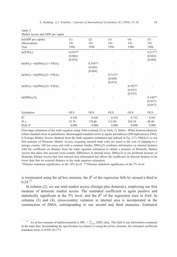
Table 2
Market access and GDP per capita
ln(GDP per capita) (1) (2) (3) (4) (5)
Observations 101 101 101 101 101
Year 1996 1996 1996 1996 1996
ln(FMAi) 0.476**
(0.066)
[0.076]
– – – 0.311**
(0.062)
[0.086]
ln(MAi) = ln(DMAi(1) + FMAi) – 0.558**
(0.042)
[0.064]
– – –
ln(MAi) = ln(DMAi(2) + FMAi) – – 0.512**
(0.048)
[0.072]
– –
ln(MAi) = ln(DMAi(3) + FMAi) – – – 0.395**
(0.023)
[0.035]
–
ln(DMAi(3)) – – – – 0.146**
(0.037)
[0.057]
Estimation OLS OLS OLS OLS OLS
R2 0.346 0.642 0.552 0.732 0.591
F(�) 52.76 174.46 112.09 294.39 48.90
Prob>F 0.000 0.000 0.000 0.000 0.000
First-stage estimation of the trade equation using Tobit (column (3) in Table 1). Huber–White heteroscedasticity
robust standard errors in parentheses. Bootstrapped standard errors in square parentheses (200 replications). FMAi
is Foreign Market Access obtained from the trade equation estimation and defined in Eq. (17); DMAi(1) is our
first measure of Domestic Market Access, assuming internal trade costs are equal to the cost of shipping to a
foreign country 100 km away and with a common border; DMAi(2) combines information on internal distance
with the coefficient on distance from the trade equation estimation to obtain a measure of Domestic Market
Access that takes into account cross-country differences in internal areas; DMAi(3) is our preferred measure of
Domestic Market Access that uses internal area information but allows the coefficient on internal distance to be
lower than that on external distance in the trade equation estimation.
*Denotes statistical significance at the 10% level. **Denotes statistical significance at the 5% level.
S. Redding, A.J. Venables / Journal of International Economics 62 (2004) 53–82 65
is reestimated using the ad hoc measure, the R2 of the regression falls by around a third to
0.24.15
In column (2), we use total market access (foreign plus domestic), employing our first
measure of domestic market access. The estimated coefficient is again positive and
statistically significant at the 5% level, and the R2 of the regression rises to 0.64. In
columns (3) and (4), cross-country variation in internal area is incorporated in the
construction of DMA, corresponding to our second and third measures. Estimated
15 An ad hoc measure of market potential is MPi ¼P
jp iGDPj=distij. This fails to use information contained
in the trade data. Reestimating the specification in column (1) using the ad hoc measure, the estimated coefficient
(standard error) is 0.958 (0.177).
S. Redding, A.J. Venables / Journal of International Economics 62 (2004) 53–8266
coefficients are positive and statistically significant at the 5% level, and with DMA(3)
included on its own, the model explains 73% of the cross-country variation in GDP per
capita. Finally, as a robustness test, column (5) enters log foreign and log domestic
market access (DMA(3)) as separate terms in the regression equation. Theory tells us
that this regression is misspecified, and we see that the R2 is lower than with the correct
specification (column (4)). However, both terms are positively signed and statistically
significant at the 5% level.
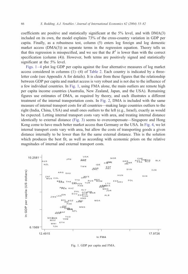
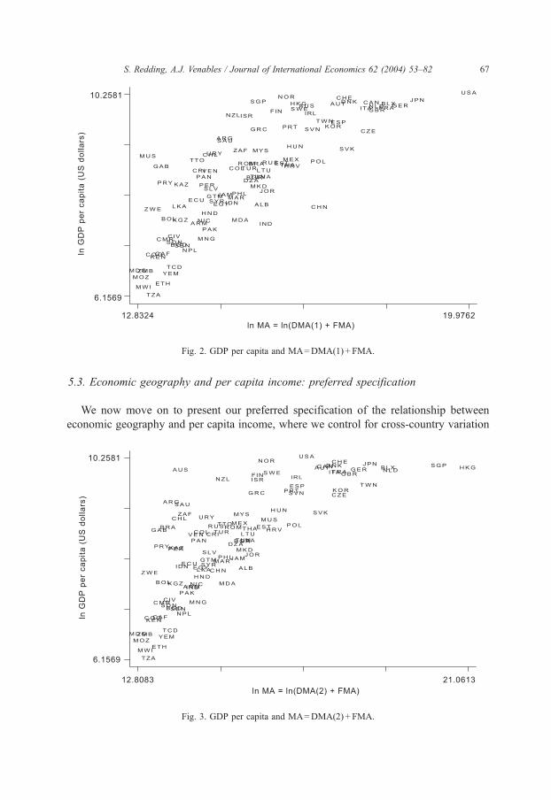
Figs. 1–4 plot log GDP per capita against the four alternative measures of log market
access considered in columns (1)–(4) of Table 2. Each country is indicated by a three-
letter code (see Appendix A for details). It is clear from these figures that the relationship
between GDP per capita and market access is very robust and is not due to the influence of
a few individual countries. In Fig. 1, using FMA alone, the main outliers are remote high
per capita income countries (Australia, New Zealand, Japan, and the USA). Remaining
figures use estimates of DMA, as required by theory, and each illustrates a different
treatment of the internal transportation costs. In Fig. 2, DMA is included with the same
measure of internal transport costs for all countries—making large countries outliers to the
right (India, China, USA) and small ones outliers to the left (e.g., Israel), exactly as would
be expected. Letting internal transport costs vary with area, and treating internal distance
identically to external distance (Fig. 3) seems to overcompensate—Singapore and Hong
Kong come to have much better market access than Germany or the USA. In Fig. 4, we let
internal transport costs vary with area, but allow the costs of transporting goods a given
distance internally to be lower than for the same external distance. This is the solution
which produces the best fit, as well as according with economic priors on the relative
magnitudes of internal and external transport costs.
Fig. 1. GDP per capita and FMA.
S. Redding, A.J. Venables / Journal of International Economics 62 (2004) 53–82 67
5.3. Economic geography and per capita income: preferred specification
We now move on to present our preferred specification of the relationship between
economic geography and per capita income, where we control for cross-country variation
Fig. 2. GDP per capita and MA=DMA(1) + FMA.
Fig. 3. GDP per capita and MA=DMA(2) + FMA.
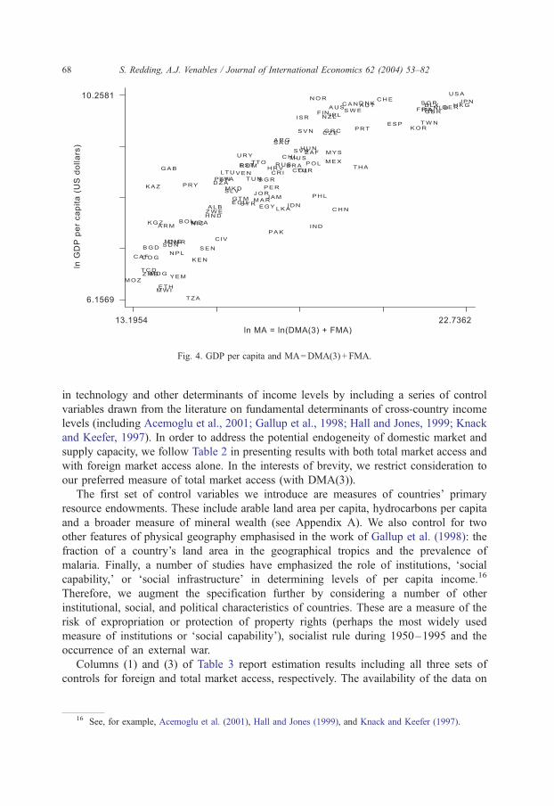
Fig. 4. GDP per capita and MA=DMA(3) + FMA.
S. Redding, A.J. Venables / Journal of International Economics 62 (2004) 53–8268
in technology and other determinants of income levels by including a series of control
variables drawn from the literature on fundamental determinants of cross-country income
levels (including Acemoglu et al., 2001; Gallup et al., 1998; Hall and Jones, 1999; Knack
and Keefer, 1997). In order to address the potential endogeneity of domestic market and
supply capacity, we follow Table 2 in presenting results with both total market access and
with foreign market access alone. In the interests of brevity, we restrict consideration to
our preferred measure of total market access (with DMA(3)).
The first set of control variables we introduce are measures of countries’ primary
resource endowments. These include arable land area per capita, hydrocarbons per capita
and a broader measure of mineral wealth (see Appendix A). We also control for two
other features of physical geography emphasised in the work of Gallup et al. (1998): the
fraction of a country’s land area in the geographical tropics and the prevalence of
malaria. Finally, a number of studies have emphasized the role of institutions, ‘social
capability,’ or ‘social infrastructure’ in determining levels of per capita income.16
Therefore, we augment the specification further by considering a number of other
institutional, social, and political characteristics of countries. These are a measure of the
risk of expropriation or protection of property rights (perhaps the most widely used
measure of institutions or ‘social capability’), socialist rule during 1950–1995 and the
occurrence of an external war.
Columns (1) and (3) of Table 3 report estimation results including all three sets of
controls for foreign and total market access, respectively. The availability of the data on
16 See, for example, Acemoglu et al. (2001), Hall and Jones (1999), and Knack and Keefer (1997).
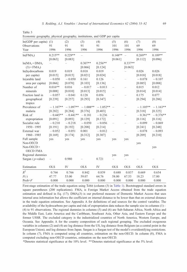
Table 3
Economic geography, physical geography, institutions, and GDP per capita
ln(GDP per capita) (1) (2) (3) (4) (5) (6) (7) (8)
Observations 91 91 91 91 101 101 69 69
Year 1996 1996 1996 1996 1996 1996 1996 1996
ln(FMAi) 0.215**
[0.063]
0.229**
[0.083]
– 0.148**
[0.061]
– 0.269**
[0.112]
0.189**
[0.096]
ln(MAi =DMAi
(3) + FMAi)
– – 0.307**
[0.066]
0.256**
[0.124]
0.337**
[0.063]
ln(hydrocarbons
per capita)
0.019
[0.015]
0.019
[0.015]
0.018
[0.021]
0.019
[0.024]
– – 0.026
[0.018]
0.026
[0.018]
ln(arable land
area per capita)
� 0.050
[0.066]
� 0.050
[0.070]
0.161
[0.103]
0.126
[0.136]
– – � 0.078
[0.085]
� 0.107
[0.088]
Number of
minerals
0.016**
[0.008]
0.016
[0.010]
� 0.017
[0.013]
� 0.013
[0.015]
– – 0.015
[0.014]
0.012
[0.014]
Fraction land in
geographical
tropics
� 0.057
[0.239]
� 0.041
[0.257]
0.128
[0.293]
0.056
[0.347]
– – 0.175
[0.294]
0.077
[0.286]
Prevalence of
malaria
� 1.107**
[0.282]
� 1.097**
[0.284]
� 1.008**
[0.376]
� 1.052**
[0.403]
– – � 1.105**
[0.318]
� 1.163**
[0.325]
Risk of
expropriation
� 0.445**
[0.091]
� 0.441**
[0.093]
� 0.181
[0.129]
� 0.236
[0.172]
– – � 0.361**
[0.116]
� 0.376**
[0.116]
Socialist rule
1950–1995
� 0.210
[0.191]
� 0.218
[0.192]
� 0.050
[0.208]
� 0.056
[0.214]
– – � 0.099
[0.241]
� 0.069
[0.248]
External war
1960–1985
� 0.052
[0.169]
� 0.051
[0.174]
0.001
[0.312]
� 0.012
[0.307]
– – � 0.078
[0.209]
� 0.093
[0.210]
Full sample yes yes yes yes yes yes
Non-OECD yes
Non-OECD+
OECD FMA
yes
Regional dummies yes yes
Sargan ( p-value) – 0.980 – 0.721 – – – –
Estimation OLS IV OLS IV OLS OLS OLS OLS
R2 0.766 0.766 0.842 0.839 0.688 0.837 0.669 0.654
F(�) 47.77 53.00 59.07 64.76 58.00 67.53 18.23 17.80
Prob>F 0.000 0.000 0.000 0.000 0.000 0.000 0.000 0.000
First-stage estimation of the trade equation using Tobit (column (3) in Table 1). Bootstrapped standard errors in
square parentheses (200 replications). FMAi is Foreign Market Access obtained from the trade equation
estimation and defined in Eq. (17); DMAi(3) is our preferred measure of Domestic Market Access that uses
internal area information but allows the coefficient on internal distance to be lower than that on external distance
in the trade equation estimation. See Appendix A for definitions of and sources for the control variables. The
availability of the hydrocarbons per capita and risk of expropriation data reduces the sample size in columns (1)–
(4) to 91 observations. The regional dummies in columns (5) and (6) are Sub-Saharan Africa, North Africa and
the Middle East, Latin America and the Caribbean, Southeast Asia, Other Asia, and Eastern Europe and the
former USSR. The excluded category is the industrialized countries of North America, Western Europe, and
Oceania. See Appendix A for the country composition of each regional grouping. The excluded exogenous
variables in columns (2) and (4) are log distance from the US, log distance from Belgium (as a central point in the
European Union), and log distance from Japan. Sargan is a Sargan test of the model’s overidentifying restrictions.
In column (7), FMA is computed using all countries, estimation on the non-OECD. In column (8), FMA is
computed excluding non-OECD countries, estimation on the non-OECD.
*Denotes statistical significance at the 10% level. **Denotes statistical significance at the 5% level.
S. Redding, A.J. Venables / Journal of International Economics 62 (2004) 53–82 69
S. Redding, A.J. Venables / Journal of International Economics 62 (2004) 53–8270
hydrocarbons per capita and the risk of expropriation reduces the sample to 91 countries.
In both cases, the estimated market access coefficient remains positively signed and highly
statistically significant. Among the control variables, the coefficients on the prevalence of
malaria and risk of expropriation are negatively signed and statistically significant at the
5% level. These findings are entirely consistent with the theoretical model presented above
if the effect of malaria and lack of protection of property rights is to reduce levels of
technical efficiency, as indeed is argued in the literature on cross-country income
differences. As an additional robustness test, we also reestimated the specification,
replacing the fraction of a country’s land area in the geographical tropics with Hall and
Jones’s (1999) measure of distance from the equator. Again, a very similar pattern of
results was observed.
In columns (2) and (4), we investigate the potential existence of other shocks to the
dependent variable that may be correlated with our measures of economic geography.
We instrument foreign and total market access with distance from the United States,
from Belgium (as a central point in the European Union), and from Japan. These capture
countries’ proximity to the three main markets and sources of supply for manufactured
goods. The instruments are highly statistically significant in the first-stage regression: for
both measures of market access, the p-value for an F-test of the null hypothesis that the
coefficients on the excluded exogenous variables are equal to zero is 0.00. In the
second-stage wage equation, we again find positive and highly statistically significant
effects of economic geography, with the IV estimate of the market access coefficients
close to those estimated using OLS.
We examine the validity of the instruments using a Sargan test of the model’s
overidentifying restrictions: for both measures of market access, we are unable to reject
the null hypothesis that the excluded exogenous variables are uncorrelated with the wage
equation residuals. These results provide evidence that the estimated market access effects
are not being driven by unmodelled (third) variables missing from our list of controls and
correlated with both market access and GDP per capita. They provide support for the
mechanisms emphasized by the theoretical model: namely, that after controlling for the
exogenous determinants of technology, distance from other countries matters for GDP per
capita through our measures of economic geography.
5.4. Robustness
Instead of seeking to model the fundamental determinants of levels of technical
efficiency, we also consider an alternative approach where replace the economic variables
with a full set of region dummies.17 The dummies control for all observed and unobserved
heterogeneity across regions, so parameters of interest are identified solely from variation
in market access within regions. Columns (5) and (6) of Table 3 report the results for
17 The regions are Sub-Saharan Africa; North Africa and the Middle East; Latin America and the Caribbean;
Southeast Asia; Other Asia; Eastern Europe and the former USSR; where the excluded category is the
industrialised countries of North America, Western Europe, and Oceania. See Appendix A for a list of the
countries included in these regions.
S. Redding, A.J. Venables / Journal of International Economics 62 (2004) 53–82 71
foreign and total market access, respectively. In each case, the estimated coefficients on all
dummy variables are negative, as is expected given the excluded category and the fact that
this is a regression for levels of per capita income. The market access coefficients remain
positive and highly statistically significant. Thus, even if we identify the relationship
between market access and per capita income using only variation within regions, we find
a positive and statistically significant effect.
One potential concern about the econometric results is that GDP per capita in one
country is being explained using measures of demand and supply capacity in other
countries (foreign market access) that are likely to be correlated with their GDP. Are the
results just picking up that rich countries tend to be located next to rich countries,
particularly within the OECD? Are our measures of transport costs (distance between
countries and the existence of a common border) really important for the results, or is
everything being driven by common shocks to GDP across countries? These concerns
have been addressed by the IV estimates in Table 3, where we have shown that distance
from the three centres of world economic activity both matters for income per capita and is
important because it affects foreign market access. However, to provide further evidence
that our results are due to the geography of access to markets and sources of supply, we
consider a number of additional robustness tests.
First, are the results being driven by the OECD? Column (7) of Table 3 reestimates the
baseline foreign market access specification for the sample of non-OECD countries,
including our full set of control variables.18 The coefficient on foreign market access
(defined as above) remains of a similar magnitude and is highly statistically significant.
Furthermore, Figs. 1–4 presented evidence of a positive relationship between GDP per
capita and market access that held at all levels of GDP per capita—for both rich and poor
countries.
Second, are the results being driven by the fact that, even outside the OECD, richer
countries tend to be located next to each other? In column (8) of Table 3, we again present
estimation results for the non-OECD, but this time, foreign market access is calculated only
using information on market capacity in OECD countries, together with distance and
common border information. Here, we examine the extent to which variation in income per
capita across non-OECD countries can be explained by differential access to OECDmarkets.
Again, we find a positive and statistically significant effect of foreign market access.
Third, are our measures of transport costs (distance between countries and the
existence of a common border) really important for the results, or is everything being
driven by common shocks to GDP across countries? As is clear from Eq. (13), market
access only varies across countries because countries have different transport cost
weights—these generate the spatial variation in market access that we use to identify
the parameters of interest. We demonstrate the importance of the transport cost weights
in two additional ways. First, by replacing a country’s true measures of distance and
the existence of a common border in the first-stage trade equation with randomly
18 Since the concern is about the industrialized OECD countries, we exclude 22 of the 23 original members
of the OECD (the missing country is Iceland which is not in our sample). The results are very similar if we instead
exclude all current OECD members.
S. Redding, A.J. Venables / Journal of International Economics 62 (2004) 53–8272
generated measures. Second, by replacing the distance and common border variables in
the first-stage trade equation with information on whether one country was a former
colony of another. These robustness tests are discussed further in the working paper
version of this paper (Redding and Venables, 2001). Each demonstrates that it is the
geography of countries’ locations relative to markets and sources of supply that is
driving our results.
Finally, as noted above, one of the advantages of using GDP information as the basis
for our left-hand side variable is that it includes the income of all immobile factors. As an
additional robustness test, we also considered a narrower definition of the income of
immobile factors based on the manufacturing wage per worker from the Unido Industrial
Statistics Database, available for a subsample of 85 countries. This yielded an extremely
similar pattern of estimation results. For example, reestimating our baseline foreign market
access specification (column (1) of Table 3) with the manufacturing wage per worker as
the left-hand side variable and our full set of controls yields an estimated coefficient
(bootstrapped standard error) of 0.239 (0.098). The corresponding estimated coefficient
(bootstrapped standard error) for our preferred measure of total market access (domestic
plus foreign, column (3) of Table 3) is 0.394 (0.109). Whether a narrow or broad definition
of the income of immobile factors is used, we find a strong relationship with measures of
economic geography.
6. Supplier access
6.1. Supplier access and intermediates goods prices
One of the key theoretical mechanisms by which location affects income per capita is
through the manufacturing price index, Gi=[SAi]1/(1� r). Countries which are remote from
sources of supply of manufactured goods incur greater transport costs, and have higher
values of the price index, Gi, reducing the wage that they can afford to pay. This provides
an independent and empirically verifiable prediction of the model. Since some cross-
country data are available on manufacturing prices, we now turn to examine this
theoretical mechanism.
Our empirical proxy for Gi is the relative price of machinery and equipment, a sector
whose output is used as an input in many other industries. The data on the relative price of
machinery and equipment are obtained from Phase V of the United Nations International
Comparisons (ICP) project (United Nations, 1994) that contains information on the price
of a large number of individual commodities in local currency units per dollar. Our
measure of the relative price of machinery and equipment is thus the PPP for machinery
and equipment divided by the PPP for GDP as a whole. Data are available for 46 countries
for the year 1985. The relative price of machinery and equipment is 1 in the United States
and reaches a maximum of 4.68 in Sri Lanka.
Table 4 presents the results of regressing the relative price of machinery and
equipment against our measure of supplier access, SAi. Column (1) considers foreign
supplier access, FSAi, alone, while column (2) introduces both domestic and foreign
supplier access using our third measure of supplier access. Column (3) presents the
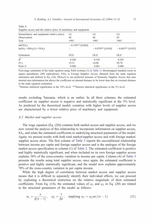
Table 4
Supplier access and the relative price of machinery and equipment
ln(machinery and equipment relative price) (1) (2) (3)
Observations 46 46 45
Year 1985 1985 1985
ln(FSAi) � 0.150** [0.060] – –
ln(SAi =DSAi(3) + FSAi) – � 0.070** [0.030] � 0.083** [0.025]
Estimation OLS OLS OLS
R2 0.260 0.192 0.283
F(�) 19.31 14.08 30.78
Prob>F 0.000 0.001 0.000
First-stage estimation of the trade equation using Tobit (column (3) in Table 1). Bootstrapped standard errors in
square parentheses (200 replications). FSAi is Foreign Supplier Access obtained from the trade equation
estimation and defined in Eq. (18). DSAi(3) is our preferred measure of Domestic Supplier Access that uses
internal area information but allows the coefficient on internal distance to be lower than that on external distance
in the trade equation estimation.
*Denotes statistical significance at the 10% level. **Denotes statistical significance at the 5% level.
S. Redding, A.J. Venables / Journal of International Economics 62 (2004) 53–82 73
results excluding Tanzania, which is an outlier. In all three columns, the estimated
coefficient on supplier access is negative and statistically significant at the 5% level.
As predicted by the theoretical model, countries with higher levels of supplier access
are characterised by a lower relative price of machinery and equipment.
6.2. Market and supplier access
The wage equation (Eq. (20)) contains both market access and supplier access, and we
now extend the analysis of this relationship to incorporate information on supplier access,
SAi, and relate the estimated coefficients to underlying structural parameters of the model.
Again, we present results with both total market/supplier access and with foreign market/
supplier access alone. The first column of Table 5 reports the unconditional relationship
between income per capita and foreign supplier access and is the analogue of the foreign
market access specification in column (1) of Table 2. The estimated coefficient is positive
and highly statistically significant, and when included on its own foreign supplier access
explains 38% of the cross-country variation in income per capita. Column (4) of Table 5
presents the results using total supplier access; once again, the estimated coefficient is
positive and highly statistically significant, and the model now explains approximately
70% of the cross-country variation in per capita income.
While the high degree of correlation between market access and supplier access
means that it is difficult to separately identify their individual effects, we can proceed
by exploiting a theoretical restriction on the relative magnitude of their estimated
coefficients. From Eq. (14), the estimated values of B1 and B2 in Eq. (20) are related
to the structural parameters of the model as follows:
u1 ¼a
bðr � 1Þ ; u2 ¼1
br; implying u1 ¼ u2ar=ðr � 1Þ ð21Þ
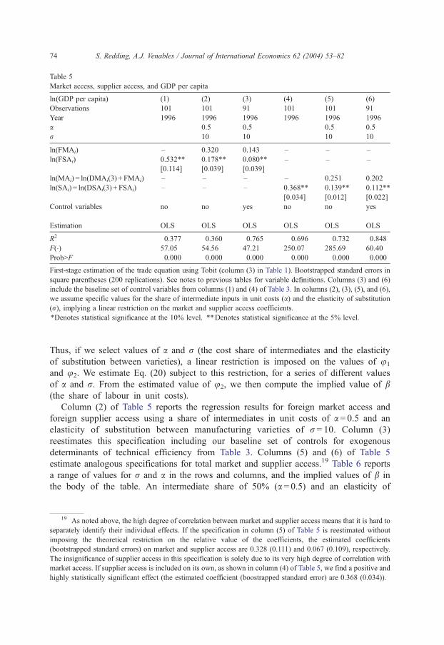
Table 5
Market access, supplier access, and GDP per capita
ln(GDP per capita) (1) (2) (3) (4) (5) (6)
Observations 101 101 91 101 101 91
Year 1996 1996 1996 1996 1996 1996
a 0.5 0.5 0.5 0.5
r 10 10 10 10
ln(FMAi) – 0.320 0.143 – – –
ln(FSAi) 0.532**
[0.114]
0.178**
[0.039]
0.080**
[0.039]
– – –
ln(MAi) = ln(DMAi(3) + FMAi) – – – – 0.251 0.202
ln(SAi) = ln(DSAi(3) + FSAi) – – – 0.368**
[0.034]
0.139**
[0.012]
0.112**
[0.022]
Control variables no no yes no no yes
Estimation OLS OLS OLS OLS OLS OLS
R2 0.377 0.360 0.765 0.696 0.732 0.848
F(�) 57.05 54.56 47.21 250.07 285.69 60.40
Prob>F 0.000 0.000 0.000 0.000 0.000 0.000
First-stage estimation of the trade equation using Tobit (column (3) in Table 1). Bootstrapped standard errors in
square parentheses (200 replications). See notes to previous tables for variable definitions. Columns (3) and (6)
include the baseline set of control variables from columns (1) and (4) of Table 3. In columns (2), (3), (5), and (6),
we assume specific values for the share of intermediate inputs in unit costs (a) and the elasticity of substitution
(r), implying a linear restriction on the market and supplier access coefficients.
*Denotes statistical significance at the 10% level. **Denotes statistical significance at the 5% level.
S. Redding, A.J. Venables / Journal of International Economics 62 (2004) 53–8274
Thus, if we select values of a and r (the cost share of intermediates and the elasticity
of substitution between varieties), a linear restriction is imposed on the values of u1
and u2. We estimate Eq. (20) subject to this restriction, for a series of different values
of a and r. From the estimated value of u2, we then compute the implied value of b(the share of labour in unit costs).
Column (2) of Table 5 reports the regression results for foreign market access and
foreign supplier access using a share of intermediates in unit costs of a= 0.5 and an
elasticity of substitution between manufacturing varieties of r = 10. Column (3)
reestimates this specification including our baseline set of controls for exogenous
determinants of technical efficiency from Table 3. Columns (5) and (6) of Table 5
estimate analogous specifications for total market and supplier access.19 Table 6 reports
a range of values for r and a in the rows and columns, and the implied values of b in
the body of the table. An intermediate share of 50% (a = 0.5) and an elasticity of
19 As noted above, the high degree of correlation between market and supplier access means that it is hard to
separately identify their individual effects. If the specification in column (5) of Table 5 is reestimated without
imposing the theoretical restriction on the relative value of the coefficients, the estimated coefficients
(bootstrapped standard errors) on market and supplier access are 0.328 (0.111) and 0.067 (0.109), respectively.
The insignificance of supplier access in this specification is solely due to its very high degree of correlation with
market access. If supplier access is included on its own, as shown in column (4) of Table 5, we find a positive and
highly statistically significant effect (the estimated coefficient (boostrapped standard error) are 0.368 (0.034)).
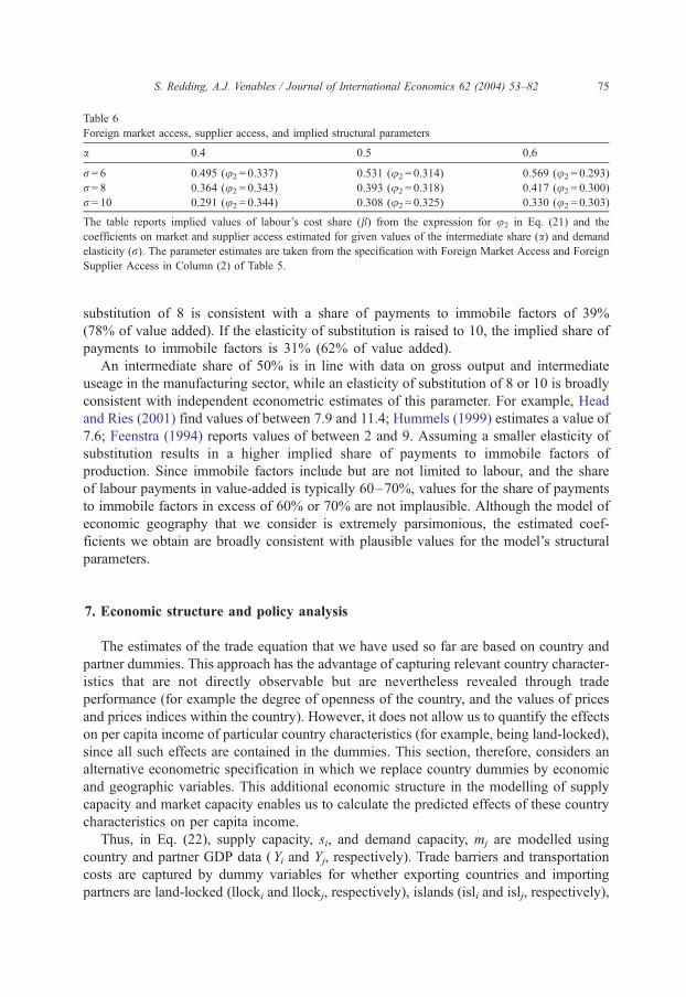
Table 6
Foreign market access, supplier access, and implied structural parameters
a 0.4 0.5 0.6
r= 6 0.495 (u2 = 0.337) 0.531 (u2 = 0.314) 0.569 (u2 = 0.293)
r= 8 0.364 (u2 = 0.343) 0.393 (u2 = 0.318) 0.417 (u2 = 0.300)
r= 10 0.291 (u2 = 0.344) 0.308 (u2 = 0.325) 0.330 (u2 = 0.303)
The table reports implied values of labour’s cost share (b) from the expression for u2 in Eq. (21) and the
coefficients on market and supplier access estimated for given values of the intermediate share (a) and demand
elasticity (r). The parameter estimates are taken from the specification with Foreign Market Access and Foreign
Supplier Access in Column (2) of Table 5.
S. Redding, A.J. Venables / Journal of International Economics 62 (2004) 53–82 75
substitution of 8 is consistent with a share of payments to immobile factors of 39%
(78% of value added). If the elasticity of substitution is raised to 10, the implied share of
payments to immobile factors is 31% (62% of value added).
An intermediate share of 50% is in line with data on gross output and intermediate
useage in the manufacturing sector, while an elasticity of substitution of 8 or 10 is broadly
consistent with independent econometric estimates of this parameter. For example, Head
and Ries (2001) find values of between 7.9 and 11.4; Hummels (1999) estimates a value of
7.6; Feenstra (1994) reports values of between 2 and 9. Assuming a smaller elasticity of
substitution results in a higher implied share of payments to immobile factors of
production. Since immobile factors include but are not limited to labour, and the share
of labour payments in value-added is typically 60–70%, values for the share of payments
to immobile factors in excess of 60% or 70% are not implausible. Although the model of
economic geography that we consider is extremely parsimonious, the estimated coef-
ficients we obtain are broadly consistent with plausible values for the model’s structural
parameters.
7. Economic structure and policy analysis
The estimates of the trade equation that we have used so far are based on country and
partner dummies. This approach has the advantage of capturing relevant country character-
istics that are not directly observable but are nevertheless revealed through trade
performance (for example the degree of openness of the country, and the values of prices
and prices indices within the country). However, it does not allow us to quantify the effects
on per capita income of particular country characteristics (for example, being land-locked),
since all such effects are contained in the dummies. This section, therefore, considers an
alternative econometric specification in which we replace country dummies by economic
and geographic variables. This additional economic structure in the modelling of supply
capacity and market capacity enables us to calculate the predicted effects of these country
characteristics on per capita income.
Thus, in Eq. (22), supply capacity, si, and demand capacity, mj are modelled using
country and partner GDP data (Yi and Yj, respectively). Trade barriers and transportation
costs are captured by dummy variables for whether exporting countries and importing
partners are land-locked (llocki and llockj, respectively), islands (isli and islj, respectively),
S. Redding, A.J. Venables / Journal of International Economics 62 (2004) 53–8276
and pursue open-trade policies (openi and openj, respectively).20 As before, the country-
partner pair specific elements of transportation costs are captured by distance between
capital cities (distij) and a dummy variable for whether or not an exporting country and
importing partner share a common border (bordij). The first-stage trade regression
therefore becomes
lnðXijÞ ¼ h þ llnðYiÞ þ klnðYjÞ þ d1lnðdistijÞ þ d2ðbordijÞ þ d3isli þ d4islj
þ d5llocki þ d6llockj þ d7openi þ d8openj þ uij: ð22Þ
This trade equation is again estimated using 1994 data and the Tobit estimator. All
variables are correctly signed according to economic priors and statistically significant at
the 5% level. The distance and land-locked variables have a negative effect on trade, while
the common border, island and Sachs and Warner (1995) openness variables have positive
effects. Predicted values of market access and supplier access are obtained from Eq. (22) in
an exactly analogous manner to before. Estimating the wage equation with both total
market/supplier access and foreign market/supplier access yields an extremely similar
pattern of results to before.21
We focus here on the effects of country characteristics on predicted income per capita.
The trade equation estimates are used to evaluate the effect of a particular economic
variable (e.g., whether a country is land-locked, or whether it pursues open-trade policies)
on market and supplier access. Combining this with the estimated coefficients from the
wage equation gives the effect of each variable on predicted income per capita. We present
predictions based on foreign market and supplier access (excluding domestic information),
assuming an intermediate share of a= 0.5 and an elasticity of substitution of r = 10 (shown
earlier to be consistent with plausible values for the share of labour in unit costs, b) andincluding our baseline set of control variables.22
Table 7 reports the results of undertaking such an analysis for five countries. Two of
these are islands, three of the countries are land-locked, and four are to some degree closed
on the Sachs and Warner (1995) definition of international openness. Changes in one
geographic or economic characteristic (such as whether a country is land-locked) have the
same proportional effect on foreign market and supplier access for all countries, and we
find that access to the coast raises predicted per capita income by 24%, while loss of island
status has a more modest effect, reducing predicted income by 7%. The effect of pursuing
open-trade policies is to raise predicted per capita income by around 25%, with the effect
now varying across countries because they differ according to their initial levels of
openness.
20 We employ the Sachs and Warner (1995) measure of international openness. This is based on tariff
barriers, non-tariff barriers, the black market exchange premium, the presence of a state monopoly on major
exports, and the existence of a socialist economic system.21 Full estimation results for the trade and wage equation are available from the authors on request.22 The use of different values for the intermediate share and elasticity of substitution has very small effects on
predictions. For example, an intermediate share of 0.5 and an elasticity of substitution of 5 raises the predicted
effect of gaining access to the coast from 24.03% to 24.08%.

Table 7
Economic magnitudes
Country Variable (%)
(1) (2) (3) (4) (5)
Access to
coast
Loss of island
status
Become
open
Distance
(Central Europe)
Distance
(50% closer to all partners)
Australia 7.34 27.06
Sri Lanka 7.34 20.66 67.40 27.06
Zimbabwe 24.03 27.65 79.74 27.06
Paraguay 24.03 25.28 58.29 27.06
Hungary 24.03 26.46 27.06
The table reports the predicted effect on GDP per capita of a change in the economic and geographical
characteristics that determine market and supplier access in the trade equation estimation (Eq. (22)). The
predictions are based on parameter estimates using Foreign Market Access and Foreign Supplier Access assuming
an intermediate share of a=0.5 and an elasticity of substitution of r=10, and including the baseline set of control
variables from column (1) of Table 3. The predicted effect of becoming open varies across countries because they
begin from different values for the Sachs and Warner (1995) openness index: 1 in Australia, 0.231 in Sri Lanka, 0
in Zimbabwe, 0.077 in Paraguay, and 0.038 in Hungary. To provide an indication of the advantages of a location
on the borders of Western Europe, column (4) reports the results of giving each country Hungary’s vector of
distances to all other countries. Column (5) reports the results of the hypothetical experiment of halving a
country’s distance from all of its trade partners.
S. Redding, A.J. Venables / Journal of International Economics 62 (2004) 53–82 77
To evaluate the quantitative importance of proximity to large markets and sources of
supply, column (4) of Table 7 undertakes the hypothetical experiment of moving three
developing countries located far from centres of world economic activity (Sri Lanka,
Zimbabwe, and Paraguay) to Central Europe.23 Gains vary from 80% for Zimbabwe to
58% for Paraguay. This emphasises the economic advantages conveyed on the transition
economies of Central and Eastern Europe by their location on the edge of high-income
Western Europe. Column (5) considers the effect of halving a country’s distance from all
of its trade partners. Once again, the gains are substantial, and the predicted increase in
income of 27% is of a similar magnitude to gaining a coastline or pursuing open-trade
policies. Increases in trade volumes are associated with these changes, so it is possible to
calculate the elasticity of income with respect to the volume of trade. On the basis of
Column (5), this elasticity is 0.23, a number comparable with the estimate of one-third
found by Frankel and Romer (1999). We stress, however, that the changes in both
income and trade are endogenous responses to the hypothetical reduction in distance.
The importance of geographical proximity is shown again in Table 8, which examines
the effect of having a common border. Common borders between Germany and the
Czech Republic and the United States and Mexico have substantial effects on predicted
income per capita in the smaller countries. Thus, removing the common border gives a
fall in predicted income per capita in the Czech Republic of 26%, and in Mexico of
27%. However, the effect of eliminating of a common border between low-income
developing countries who trade relatively little with one another, such as Zimbabwe and
Zambia, is small. This suggests that the gains from closer regional integration between
23 Specifically, we replace a country’s distance and common border vectors by those of Hungary.
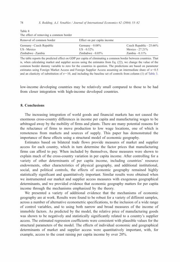
Table 8
The effect of removing a common border
Removal of common border Effect on per capita income
Germany–Czech Republic Germany –0.08% Czech Republic –25.66%
US–Mexico US –0.52% Mexico –27.21%
Zimbabwe–Zambia Zimbabwe –0.05% Zambia –0.11%
The table reports the predicted effect on GDP per capita of eliminating a common border between countries. That
is, when calculating market and supplier access using the estimates from Eq. (22), we change the value of the
common border dummy variable to zero for the countries in question. The predictions are based on parameter
estimates using Foreign Market Access and Foreign Supplier Access assuming an intermediate share of a=0.5and an elasticity of substitution of r=10, and including the baseline set of controls from column (1) of Table 3.
S. Redding, A.J. Venables / Journal of International Economics 62 (2004) 53–8278
low-income developing countries may be relatively small compared to those to be had
from closer integration with high-income developed countries.
8. Conclusions
The increasing integration of world goods and financial markets has not caused the
enormous cross-country differences in income per capita and manufacturing wages to be
arbitraged away by the mobility of firms and plants. There are many potential reasons for
the reluctance of firms to move production to low wage locations, one of which is
remoteness from markets and sources of supply. This paper has demonstrated the
importance of these effects using a structural model of economic geography.
Estimates based on bilateral trade flows provide measures of market and supplier
access for each country, which in turn determine the factor prices that manufacturing
firms can afford to pay. When included by themselves, these measures were shown to
explain much of the cross-country variation in per capita income. After controlling for a
variety of other determinants of per capita income, including countries’ resource
endowments, other characteristics of physical geography, and additional institutional,
social, and political controls, the effects of economic geography remained highly
statistically significant and quantitatively important. Similar results were obtained when
we instrumented our market and supplier access measures with exogenous geographical
determinants, and we provided evidence that economic geography matters for per capita
income through the mechanisms emphasized by the theory.
We presented a variety of additional evidence that the mechanisms of economic
geography are at work. Results were found to be robust for a variety of different samples,
across a number of alternative econometric specifications, to the inclusion of a wide range
of control variables, and to using both narrow and broad measures of the income of
immobile factors. As predicted by the model, the relative price of manufacturing goods
was shown to be negatively and statistically significantly related to a country’s supplier
access. The estimated regression coefficients were consistent with plausible values for the
structural parameters of the model. The effects of individual economic and geographical
determinants of market and supplier access were quantitatively important, with, for
example, access to the coast raising per capita income by over 20%.
S. Redding, A.J. Venables / Journal of International Economics 62 (2004) 53–82 79
Our results may seem rather pessimistic for developing countries, suggesting that even
if tariff and institutional obstacles to trade and investment are removed the penalty of
distance will continue to hold down the incomes of remote regions. However, it is
important to recall that our results are derived for a given location of production and
expenditure. As new markets and centres of manufacturing activity emerge, so the market
and supplier access of neighbouring countries improves. Our results point to the importance
of understanding the role of geography in shaping the evolution of the cross-country
distribution of income.
Acknowledgements
This paper is produced as part of the Globalization programme of the ESRC funded
Centre for Economic Performance at the LSE. Redding gratefully acknowledges financial
support from a Philip Leverhulme Prize. We are grateful to two anonymous referees,
Andrew Bernard, Tim Besley, Jonathan Eaton, Masahisa Fujita, Gordon Hanson, James
Harrigan, David Hummels, Sam Kortum, Edward Leamer, Tomoya Mori, Stephen Nickell,
Henry Overman, Steve Pischke, Dani Rodrik, Peter Schott, Jon Temple, Alan Winters, and
seminar participants at the CEPR European Research Workshop in International Trade
(Copenhagen), Empirical Issues in International Trade (Boulder), European Trade Study
Group (Glasgow), Bocconi University, Boston University, Hitotsubashi University, Kobe
University, Kyoto University, London School of Economics, New York Federal Reserve,
Osaka University, University of Texas, University of Bristol, University of Oxford,
University of Warwick, and World Bank for helpful comments. Thanks also to Alessandro
Nicita, Martin Stewart, and Mercedes Vera-Martin for research assistance, and to Charles
Jones, Phillip Parker, and Jeffrey Sachs for making their data available to us. The usual
disclaimer applies.
Appendix A
Bilateral Trade: data on bilateral trade flows are from the World Bank COMTRADE
database. This provides information for the 101 countries listed below during 1992–1996.
GDP per capita: data on current price (US dollars) GDP and on population are from
the World Bank and are available for the 101 countries listed below during 1992–1996.
Geographical variables: data on bilateral distance, internal area, arable land area,
existence of a common border, and whether a country is an island or land-locked are from
the World Bank. These data are also available for the 101 countries listed below.
Manufacturing wage per worker: data on number of employees and wages and
salaries (current price US dollars) in total manufacturing are from the UNIDO Industrial
Statistics Database. Information is available for 85 countries during 1992–1996.
Relative price of machinery and equipment: data on the price of machinery and
equipment and GDP in local currency units per US dollar are from Phase V of the United
Nations International Comparisons Project (United Nations, 1994). The data are available
for 46 countries and are for 1985.
S. Redding, A.J. Venables / Journal of International Economics 62 (2004) 53–8280
Number of Minerals: the total number of minerals of which a country has reserves
from the list of 44 main minerals compiled by Parker (1997).
Risk of Expropriation: extent of protection of property rights, measured on a scale
from 1 to 5, where a higher score indicates weaker protection of property rights. Source:
Holmes et al. (1997). These data are unavailable for Central African Republic, Guatemala,
Kazakhstan, Kyrgyz Republic, Madagascar, Macedonia, Mauritius, and Chad.
Physical Geography and Institutional, Social, and Political Characteristics: data on
hydrocarbons (deposits of petroleum and natural gas) per capita, fraction of land area in
the geographical tropics, prevalence of malaria, socialist rule, and the occurrence of an
external war are from Gallup et al. (1998). Information is available for all 101 countries in
our data set, except for the data on hydrocarbons per capita which are unavailable for
Moldova and Yemen. The data can be downloaded from http://www.cid.harvard.edu/
ciddata.ciddata.html.
International Openness: data on international openness are from Sachs and Warner
(1995) and are available for 98 countries. Information is unavailable for Panama, Saudi
Arabia, and Yemen (see http://www.cid.harvard.edu/ciddata.ciddata.html).
Sub-Saharan Africa: Central African Republic, Cote d’Ivoire, Cameroon, Congo
Republic, Ethiopia, Gabon, Kenya, Madagascar, Mozambique, Mauritius, Malawi, Sudan,
Senegal, Chad, Tanzania, South Africa, Zambia, and Zimbabwe.
North Africa and the Middle-East: Algeria, Egypt, Israel, Jordan, Morocco, Saudi
Arabia, Syria, Tunisia, and Yemen.
Latin America and the Caribbean: Argentina, Bolivia, Brazil, Chile, Colombia,
Costa Rica, Ecuador, Guatemala, Honduras, Jamaica, Mexico, Nicaragua, Panama, Peru,
Paraguay, El Salvador, Trinidad and Tobago, Uruguay, and Venezuela.
Southeast Asia: China, Hong Kong, Indonesia, Japan, Korea, Malaysia, Philippines,
Singapore, Thailand, and Taiwan.
Other Asia: Bangladesh, India, Sri Lanka, Mongolia, Nepal, and Pakistan.
Eastern Europe and the former USSR: Albania, Armenia, Bulgaria, Czech Republic,
Estonia, Croatia, Hungary, Kazakhstan, Kyrgyz Republic, Lithuania, Latvia, Moldova,
Macedonia, Poland, Romania, Russia, Slovak Republic, and Slovenia.
Country codes: Albania (ALB), Argentina (ARG), Armenia (ARM), Australia (AUS),
Austria (AUT), Bangladesh (BGD), Bulgaria (BGR), Belgium/Luxembourg (BLX),
Bolivia (BOL), Brazil (BRA), Central African Republic (CAF), Canada (CAN), Switzer-
land (CHE), Chile (CHL), China (CHN), Cote d’Ivoire (CIV), Cameroon (CMR), Congo
Republic (COG), Columbia (COL), Costa Rica (CRI), Czech Republic (CZE), Germany
(DEU), Denmark (DNK), Algeria (DZA), Ecuador (ECU), Egypt (EGY), Spain (ESP),
Estonia (EST), Ethiopia (ETH), Finland (FIN), France (FRA), Gabon (GAB), UK (GBR),
Greece (GRC), Guatemala (GTM), Hong Kong (HKG), Honduras (HND), Croatia (HRV),
Hungary (HUN), Indonesia (IDN), India (IND), Ireland (IRL), Israel (ISR), Italy (ITA),
Jamaica (JAM), Jordan (JOR), Japan (JPN), Kazakhstan (KAZ), Kenya (KEN), Kyrgyz
Republic (KGZ), South Korea (KOR), Sri Lanka (LKA), Lithuania (LTU), Latvia (LVA),
Morocco (MAR), Moldova (MDA), Madagascar (MDG), Mexico (MEX), Macedonia
(MKD), Mongolia (MNG), Mozambique (MOZ), Mauritius (MUS), Malawi (MWI),
Malaysia (MYS), Nicaragua (NIC), Netherlands (NLD), Norway (NOR), Nepal (NPL),
New Zealand (NZL), Pakistan (PAK), Panama (PAN), Peru (PER), Philippines (PHL),
S. Redding, A.J. Venables / Journal of International Economics 62 (2004) 53–82 81
Poland (POL), Portugal (PRT), Paraguay (PRY), Romania (ROM), Russia (RUS), Saudi
Arabia (SAU), Sudan (SDN), Senegal (SEN), Singapore (SGP), El Salvador (SLV),
Slovak Republic (SVK), Slovenia (SVN), Sweden (SWE), Syria (SYR), Chad (TCD),
Thailand (THA), Trinidad and Tobago (TTO), Tunisia (TUN), Turkey (TUR), Taiwan
(TWN), Tanzania (TZA), Uruguay (URY), United States of America (USA), Venezuela
(VEN), Yemen (YEM), South Africa (ZAF), Zambia (ZMB), and Zimbabwe (ZWE).
References
Acemoglu, D., Johnson, S., Robinson, J., 2001. The colonial origins of comparative development: an empirical
investigation. American Economic Review 91 (5), 1369–1401.
Anderson, J., van Wincoop, E., 2003. Gravity with gravitas: a solution to the border puzzle. American Economic
Review 93 (1), 170–192.
Combes, P., Lafourcade, M., 2001. Transport cost decline and regional inequalities: evidence from France. CEPR
Discussion Paper, vol. 2894.
Efron, B., Tibshirani, R., 1993. An introduction to the bootstrap. Monographs on Statistics and Applied Prob-
ability. Chapman & Hall, New York.
Feenstra, R., 1994. New product varieties and the measurement of international prices. American Economic
Review 84 (1), 157–177.
Frankel, J., Romer, D., 1999. Does trade cause growth? American Economic Review 89 (3), 379–399.
Fujita, M., Krugman, P., Venables, A.J., 1999. The Spatial Economy: Cities, Regions, and International Trade.
MIT Press, Cambridge, MA.
Gallup, J., Sachs, J., Mellinger, A., 1998. Geography and economic development. Proceedings of Annual World
Bank Conference on Development Economics. World Bank, Washington D.C., pp. 127–178.
Hall, R., Jones, C., 1999. Fundamental determinants of output per worker across countries. Quarterly Journal of
Economics 114 (1), 83–116.
Hanson, G., 1998. Market potential, increasing returns and geographic concentration. NBER Working Paper,
vol. 6429.
Harris, C., 1954. The market as a factor in the localization of industry in the United States. Annals of the
Association of American Geographers 64, 315–348.
Head, K., Ries, J., 2001. Increasing returns versus national product differentiation as an explanation for the
pattern of US–Canada trade. American Economic Review 91 (4), 858–876.
Holmes, K., Johnson, B., Kirkpatrick, M., 1997. 1996 Index of Economic Freedom. The Heritage Foundation and
The Wall Street Journal, Washington DC and New York.
Hummels, D., 1995. Global income patterns: does geography play a role? Chapter 2 of PhD Thesis, University of
Michigan.
Hummels, D., 1999. Towards a geography of trade costs. University of Chicago, mimeograph.
Knack, S., Keefer, P., 1997. Does social capital have an economic payoff? Quarterly Journal of Economics 112,
1251–1288.
Leamer, E., 1997. Access to Western markets and Eastern effort. In: Zecchini, S. (Ed.), Lessons from the
Economic Transition, Central and Eastern Europe in the 1990s. Kluwer Academic Publishing, Dordrecht,
pp. 503–526.
Limao, N., Venables, A.J., 2001. Infrastructure, geographical disadvantage, transport costs, and trade. World
Bank Economic Review 15, 451–479.
Overman, H.G., Redding, S., Venables, A.J., 2003. The economic geography of trade, production and income: a
survey of empirics. In: Kwan-Choi, E., Harrigan, J. (Eds.), Handbook of International Trade. Basil Blackwell,
Oxford, pp. 353–387.
Pagan, A., 1984. Econometric issues in the analysis of regressions with generated regressors. International
Economic Review 25 (1), 221–247.
Parker, P., 1997. National cultures of the world: a statistical reference. Cross-Cultural Statistical Encyclopedia of
the World, vol. 4. Greenwood Press, Westport CT.
S. Redding, A.J. Venables / Journal of International Economics 62 (2004) 53–8282
Radelet, S., Sachs, J., 1998. Shipping costs, manufactured exports and economic growth. Paper presented at the
American Economic Association Meetings, Chicago. Mimeograph.
Redding, S., Venables, A.J., 2001. Economic geography and international inequality. CEP Discussion Paper 495.
London School of Economics.
Sachs, J., Warner, A., 1995. Economic reform and the process of global integration. Brookings Papers on
Economic Activity (1), 1–95.
United Nations, A., 1994. World Comparisons of Real Gross Domestic Product and Purchasing Power, 1985:
Phase V of the International Comparisons Programme. United Nations, New York.