0

15/8/18

Economic Geography and Trade*

Anthony J. Venables

Dept of Economics

University of Oxford

Summary

Economic activity is unevenly distributed across space, both internationally and within

countries. What determines this spatial distribution, and how is it shaped by trade? Classical

trade theory gives the insights of comparative advantage and gains from trade, but is firmly

aspatial, modelling countries as points and trade (in goods and factors of production) as either

perfectly frictionless or impossible. Modern theory places this in a spatial context in which

geographical considerations influence the volume of trade between places. Gravity models

tell us that distance is important, with each doubling of distance between places halving the

volume of trade. Modelling the location decisions of firms gives a theory of location of

activity based on factor costs (as in classical theory), and also on proximity to markets,

proximity to suppliers, and the extent of competition in each market. It follows from this that

– if there is a high degree of mobility – firms and economic activity as a whole may tend to

cluster, providing an explanation of observed spatial unevenness. In some circumstances

falling trade barriers may trigger the deindustrialisation of some areas as activity clusters in

fewer places. In other circumstances falling barriers may enable activity to spread out,

reducing inequalities within and between countries. Research over the last several decades

has established the mechanisms that cause these changes and placed them in full general

equilibrium models of the economy. Empirical work has quantified many of the important

relationships. However, geography and trade remains an area where progress is needed to

develop robust tools that can be used to inform place-based policies (concerning trade,

transport, infrastructure and local economic development), particularly in view of the huge

expenditures that such policies incur.

Keywords: Economic geography, trade, globalisation, agglomeration, clustering.

JEL classification: F1, F2, F6, R1.

* Forthcoming, Oxford Research Encyclopedia of Economics and Finance

1

Introduction

Spatial unevenness is a striking characteristic of the world economy. Per capita income

levels vary across countries by a factor of more than a hundred to one: within countries

population and economic activity concentrate in cities that cover a small fraction of the

national land area: global activity in some sectors – finance, high-tech, film-making – is

concentrated in relatively few cities. Some of this is explained by physical geography but

most of it is the outcome of economic processes. Textbook economic principles offer no

explanation of this unevenness; under the standard assumptions of general equilibrium theory

economic activity will tend to smear more or less uniformly across space. A recent literature

combining insights from economic geography and from trade theory does offer an

explanation, showing how trade may create spatial structures which are highly uneven.

Relatively uniform distribution of activity may not be a (stable) equilibrium as clustering

occurs.

This paper reviews the theory and the implications that flow from it. The central question to

be addressed is: what determines the location of economic activity? The question can be

posed at different spatial levels: location across nations, across regions, cities, or within a

particular city. And it can be posed of different economic variables: the location of people or

the location of jobs, in aggregate or in different sectors. The answer is important because the

spatial distribution of income and prosperity follows from it. This paper focuses on the

international angle and on why some places are more attractive locations for production – and

hence offer higher wages and incomes – than others.

As usual in economics, the fundamental determinants are endowments, technology, and

preferences. At a point in space these are natural resources, stocks of labour and capital,

available technologies and institutions, and the preferences of inhabitants. Trade and

economic geography bring the extra ingredient of spatial interaction, determined by the

mobility of factors of production, technology, and the goods and services that they produce.

The spatial scale of mobility varies, with labour moving freely within a country but generally

not between countries; capital flows between countries but is often subject to regulation; the

mobility of goods and services spans the spectrum from instantaneous global transmission of

digital products to non-tradable supply of haircuts and restaurant meals. The impact of these

spatial interactions depends on the economic environment in which they occur. Ideas can

2

move quite freely but the absorptive capacity of a firm or country to employ them varies

widely. The effect of integrating separate national goods or service markets depends on

characteristics of the regions that are integrating, and of the sectors that are being integrated.

The tasks facing researchers in economic geography and trade are therefore twofold. (i) To

understand the form and extent of spatial interactions – what is mobile, what is immobile, and

why? (ii) To understand the implications of these interactions for the spatial distribution of

activity and prosperity, recognising the heterogeneity of types of interaction and of the

economic environments in which they occur.

Partial answers to these questions come from the classic models of international trade dating

back to Ricardo and the works of Heckscher and Ohlin. These models (at least in their

current textbook form, e.g. Krugman et al. 2015) concentrate on trade in final goods, trade

being driven by international differences in technology (Ricardo) or endowments (Heckscher-

Ohlin). These models give us the key insights of comparative advantage and the gains from

trade. However, they have no geography – countries are ‘points’ and mobility is either

assumed to be perfect (frictionless trade in goods) or impossible (factor assumed immobile).1

The economic environment of these models is one of constant returns to scale and perfect

competition. These assumptions limit the set of questions that can be addressed, and also

mean that the approach offers little insight into three predominant features of trade and

economic geography. One is that most international trade flows are curtailed sharply by

distance. The second is the presence of intra-industry trade – two-way trade flows in similar

products between similar economies. And the third is spatial unevenness in economic

activity.

Developments in economic geography and trade have gone a long way to fill these gaps. The

‘new’ trade theory of the 1980s adds imperfect competition and increasing returns, focusing

attention on the behaviour of firms. This provides a theory of intra-industry trade, and also a

framework in which to analyse the location decisions of firms. Building on this it became

apparent that sufficiently high levels of spatial interaction – or to put it crudely, sufficiently

many things being mobile – create the possibility that economic activity will tend to

concentrate in relatively few places. In some circumstances trade is a driver of convergence

between places, and in others causes divergence and creates spatial unevenness.

3

This paper provides a selective overview of this literature and the main results and insights

that come from it. The overview is non-technical, giving references to previously published

technical surveys. The next section of the paper deals with the geographical pattern of trade

flows; it is largely empirical, but establishes the point that geography matters for trade. The

following section turns to theory, outlining a basic model of location of ‘industry’.

Throughout the paper the term ‘industry’ is used to cover productive activities whose location

is not fixed by dependence on natural resources (agriculture or mining) or by servicing

geographically fixed assets (e.g. provision of utilities); it therefore covers manufacturing and

large parts of the service sector. Following this the paper discusses applications of the theory

and empirics, finally turning to directions for future research.

The Geography of Trade

The point of departure for studying economic geography and trade is to look at the economic

geography of trade. The overwhelming feature is that trade flows are sharply curtailed by

distance. Thus, the UK trades more with Ireland than it does with China, an economy fifty

times larger. Geography and spatial frictions evidently matter for trade and the tool for

researching them is the ‘gravity model’, first written down by Jan Tinbergen in 1962.

Stripped down to essentials, it says that the value of trade between two countries is

approximated by the relationship

jiijij ZZdFX ,, . (1)

Xij are the exports from i to j, dij are ‘between-country’ characteristics, in particular the

distance between the two countries, Zi are exporter country characteristics, and Zj importer

country features. A relationship of this type is consistent with a number of theoretical

underpinnings providing that there are some trade frictions between countries and some

reason for trade.2

There is good data on bilateral goods trade between most countries in the world so this

relationship can be econometrically estimated. The simplest form is to assume the

relationship is log-linear, use distance as the only between-country variable and GDP as the

exporter and importer country characteristics. A thorough exposition of these models, the

technical issues involved and the main results is contained in Head and Mayer (2014), on

which following paragraphs draw.

4

The coefficients on income are generally close to unity, and the coefficient on distance is

close to minus one.3 This implies that the effects of distance are large: trade volumes are

proportional to the reciprocal of distance so each doubling of distance halves the volume of

trade (conditional on GDP). The relationship is typically estimated on aggregate goods trade

and across a wide range of countries so coefficients are average effects. These mask a lot of

heterogeneity – trade in oil is quite different from trade in motor vehicle parts. Estimating

the relationship for service trade is hard as bilateral service trade data is not widely available,

although estimates suggest that the effect of distance is only slightly less for services than for

goods trade. There are some estimates of internet trade, giving estimates of the gravity

coefficient about 2/3rds that of corresponding trade flows (Lendle et al. 2016).

Many other variables have been added to the minimal version sketched above. Additional

between-country measures include contiguity (+, indicating more trade), common language

(+), colonial relationship (+), membership of a common regional integration agreement (+),

common currency (+). Further measures of exporter and importer country characteristics

include land area (-) and division of aggregate GDP into population and per capita GDP, both

positive and the latter larger than the former.

Finally, there is evidence that the absolute value of the distance coefficient has increased over

time, rising from around 0.95 in the 1970s to around 1.1 in recent studies (Disdier and Head,

2008). This seems surprising, particularly in view of popular writings on the death of

distance (e.g. Cairncross, 1997), but it should be borne in mind that this is a slope coefficient

and the intercept of the relationship was increasing through most of the period; trade was

increasing relative to GDP, but long-distance trade increased less rapidly than short-distance.

These findings all indicate substantial geographical trade frictions. What underpins them?

Numerous mechanisms can be posited although empirical study has not been successful in

establishing the relative importance of each. Transport costs are the most obvious. Research

suggests that the elasticity of transport costs with respect to distance is less than unity while

the elasticity of trade with respect to transport costs is greater than unity (absolute value),

these combining to give the trade/ distance coefficient of -1. Time in transit is important, and

has probably become more so with the rise of international production networks. The

importance of just-in-time delivery in these and other trades is put forward as one reason for

the increase in the absolute value of the distance coefficient through time. Perhaps the most

5

important factor, if hard to quantity, is a package of costs of doing business at a distance.

Firms and traders are likely to have better information about nearby markets than remote

ones; it is easier transacting in similar time zones; face-to-face contact is important for

building trust in relationships, and so on.

The Location of Activity: Theory

Geography matters for trade, and trade matters for shaping economic geography. To capture

this a theory of location of economic activity is needed. Classical trade theory offers a

theory, but as noted above, its assumptions proved too restrictive to provide insight into many

important phenomena. In particular, the rise in the volume of intra-industry trade that

occurred in the post-war period is not readily explained by models of trade under perfect

competition. This fact, together with the increasing returns revolution in economic theory

that took place in the 1980s, led to a change in the focus of trade theory with the ‘new trade

theory’.

There are several ingredients, of which the most important is the focus on firms. Firms are

modelled as having economies of scale (this giving them finite size and implying marginal

cost below average cost); as having some market power, so able to price above marginal cost;

and typically deriving this market power from product differentiation, modelled in the style

pioneered by Dixit and Stiglitz (1977). Production sectors are typically modelled as

monopolistically competitive, i.e. with the number of constituent firms determined by free

entry/ exit until a zero profit condition is satisfied. The approach provides a fertile

framework for addressing numerous issues. Intra-industry trade arises naturally as each firm

can make profit by selling its product in each market. Such trade is consistent with the

gravity relationship as, given likely price elasticities of demand for the products of particular

firms, quite small trade frictions have a large impact on trade volumes. The framework

enabled rich seams of work on foreign direct investment (Markusen, 2002) and on firm level

heterogeneity, the latter using micro-level datasets (Melitz and Redding, 2014).

The approach also provides a framework for analysing firms’ location decisions and hence

the economic geography of trade and production. The different forces at work can be

illustrated for a single industry in a simple reduced form framework. A single firm in country

i has sales volume in country j expressed as jiijij mcdfx ,, . Sales are a decreasing with

6

distance, dij, and with costs of production in country i, ci, since both of these increase the

price of goods supplied from i to j. However, they are an increasing function of the ‘market

capacity’ of country j market, denoted mj. Market capacity is the size of the country j market

(expenditure in the sector under study) combined (inversely) with a measure of market

crowdedness, i.e. the competitive pressure from other firms that supply this market.4

The total sales of a country i firm across all markets are j jiiji mcdfx ,, and, in models

of this type, each firm breaks-even if sales reach a particular level, x , making positive profits

if sales exceed this and losses if they are less. 5 The number of firms in country i is denoted

in , and the monopolistic competition setting means that there is entry of country i firms,

denoted 0 in , if profits are positive, and exit, 0 in , if firms are loss making, so

xmcdfxxnj jiijii ,, . (2)

Equilibrium is when the number of firms has adjusted such that 0 in for all i.

The mechanisms that bring about this equality are dependence of costs ci and market capacity

mj, on the number of firms, in .6 The remainder of this section outlines four forces that drive

this dependency and hence ensure that equation (2) is equal to zero.

Factor Costs

The first mechanism – and that akin to classical trade theory – is that factor prices and costs

of production in the country are increasing in the scale of operation of the industry, so ci is

increasing in ni. Thus, the scale of activity in country i, as represented by the number of

firms, ni, increases until wages and costs are bid up to the point where no further entry is

profitable. This obviously depends on the size, productivity, and elasticity of supply of

factors of production used in country i.

Market Size and Market Crowding

Entry of firms will not only bid up factor prices in the producing country, but also increase

supply and therefore reduce prices in markets to which they export. Thus, market capacity mj

is a decreasing function of the number of firms in each of the countries that export to country

j.7 If all countries are identical the solution is easy to see. The same number of firms

7

operates in each country, and the number is such that factor prices and output prices have

jointly adjusted to make equation (2) equal to zero.

What if countries are not symmetric? If one country is α% larger than another, one might

guess that it has α% more firms, and this would be correct if each country’s firms took the

same share of each market. But if there are trade frictions and gravity holds, then firms have

a larger share of their home market than of their export markets. The larger country must

then have more than α% of the world’s firms, as its firms have the largest share in the largest

market. This is sometimes referred to as the home market effect, and it means that large

centres (in different contexts large cities, regions or countries) are advantaged by the

geography of gravity. The advantage takes some combination of larger countries having

disproportionately more firms and, if factor prices are increasing in the number of firms, also

having higher wages and higher real incomes. Empirical support for this effect is discussed

later in this paper.8

Factor Mobility

A further mechanism comes into play if factors of production – labour in particular – is

mobile between places. The home market effect discussed in the previous paragraph suggests

that a large country might have higher wages and real incomes. With labour mobility, this

attracts immigrants, further enlarging the size of the market (tending to increase market

capacity, mi) and perhaps also mitigating increasing factor costs (reducing ci). If this effect

is strong enough then the right-hand side of equation (2) becomes an increasing function of

the number of firms ni, so that having more firms creates a force for attracting still more.

This mechanism is the driver of the ‘core-periphery’ model of Krugman (1991). The

simplest version of this model has two regions that are identical in their underlying structure

and parameters, and some workers and firms that are mobile between regions. Symmetry of

structure and parameters means that there is always a symmetric equilibrium with the same

number of firms in each region, but this may be unstable – if one region gets slightly larger it

will attract firms and migrants and become still larger. In addition to the unstable symmetric

equilibrium there are therefore two asymmetric equilibria, in which all firms have moved to

either one region or the other. The model provides no prediction as to which might occur, but

makes the fundamental point that spatial interactions can create divergence in economic

outcomes between places that have identical economic fundamentals.

8

Linkages, Intermediate Goods, and Clusters

The combination of the home market effect and labour mobility create the possibility that the

right-hand side of (2) is increasing in ni. Other mechanisms, perhaps more relevant in the

international context, can have the same effect. One such mechanism is the presence of

intermediate goods, produced under conditions of product differentiation and monopolistic

competition (Venables, 1996). More firms in a place mean a larger market for intermediate

goods (a backwards linkage creating a larger market capacity, mi for suppliers of

intermediates). This attracts firms that supply intermediate goods, and proximity of suppliers

to users brings a cost reduction (a forward linkage creating a lower ci) for firms using the

goods. This reinforces the attractiveness of the place for final goods production setting off

the process of cumulative causation and clustering of industry in one place.

This is one example of a wider set of agglomeration economies that are generated by close

and intense economic interaction and have the effect of raising productivity in affected areas

and activities. They arise through several different mechanisms.9 Thick labour markets

enable better matching of workers to firms’ skill requirements. Better communication

between firms and their customers and suppliers enables knowledge spillovers, better product

design and timely production. A larger local market enables development of a larger network

or more specialised suppliers. Fundamentally, larger and denser markets allow for both scale

and specialisation. A good example is given by specialist workers or suppliers. The larger

the market the more likely it is to be worthwhile for an individual to specialise and hone

skills in producing a particular good or service. The presence of highly specialised skills will

raise overall productivity. The specialist will be paid for the product or service supplied but,

depending on market conditions, is unlikely to capture the full benefit created.10 Since the

benefit is split between the supplier and her customers there is a positive externality. And

this creates a positive feedback – more firms will be attracted to the place to receive the

benefit, growing the market, further increasing the returns to specialisation, and so on. This

is the classic process of cluster formation.

These mechanisms have both a spatial and a sectoral range. They may be sector specific, tied

to particular labour skills, firm capabilities, or input-output linkage (in which case they are

sometimes referred to as ‘localisation’ or ‘Marshall-Romer’ economies) or may operate

across many sectors (in the regional economics literature referred to as ‘urbanisation’ or

9

‘Jacobs’ economies). They are developed rigorously in the literature, being given micro-

economic foundations and set in a full general equilibrium framework in which not only the

determinants but also the full implications of location choices are established.

To summarise, economic geography and trade gives a theory of industrial location

determined by four mechanisms:

i) Factor costs, in turn a function of endowments and technology.

ii) Market access; trade costs, proximity, market size and market crowding

iii) Supplier access and agglomeration; proximity to suppliers of intermediate goods and

other complementary activities or sources of technological spillovers.

iv) Factor mobility: the mobility of factors of production, feeding back to influence

endowments and market size.

The first of these is the subject of classic trade theory, and the second adds trade frictions and

gravity. Together they imply diminishing returns to expanding activity, and hence unique

and stable equilibria. The third and fourth are at the centre of economic geography. They

create positive feedbacks and hence the potential for multiple equilibria and the clustering of

economic activity.11

Issues and Applications

The approaches outlined in the preceding section have been applied to a number of issues,

three of which are outlined in this section, starting with international inequalities, turning to

emergent structure, and ending with trade and economic development.

Trade and International Inequalities

A central concern of much work in economic geography has been imbalance between

successful and lagging regions. This may be within countries or, in the international context,

shaping global inequalities and economic development. Central questions are: how does

openness to trade affect international inequalities? In what circumstances do some countries

benefit from trade while others lose, in relative or absolute terms?

The simplest economic geography framework for addressing this question is a world

containing two countries and, to address the question in its purest form, the countries are

10

assumed to have identical fundamentals.12 Each country has a single factor of production

(labour, which is internationally immobile), and may potentially have activity in two sectors.

One is perfectly competitive, operates under constant returns to scale and is freely traded.

The other is an industrial sector, monopolistically competitive as sketched in the previous

section. This sector also has the feature that its output is used both as final consumer goods

and as intermediates in the same sector. Thus, inputs to ‘industry’ are both labour and

industrial products; and the output of industry is partly for final consumption and partly

intermediate inputs for industry.13 What happens as the cost of trading industrial goods

between countries are reduced?

This is a model in which mechanisms (ii) and (iii) of the list above operate, but mechanisms

(i) and (iv) are switched off. This captures the ‘fundamental trade-off in spatial economics’,

between costs of mobility and various types of scale economies (Fujita and Thisse 2002).

Mechanism (ii) is a force for dispersion of activity; given that there are consumers in both

countries and trade costs, firms want to locate in both countries. Mechanism (iii) is a force

for concentration and clustering; firms want to be close to supplier firms and customer firms.

How does the balance change as trade barriers are reduced?

At prohibitively high trade costs industry must be located in both countries in order to meet

the demands of consumers so, if the countries have identical fundamentals the equilibrium

will be symmetric, with production equally divided and both economies identical. As trade

costs are reduced so there is intra-industry trade and consumers and producers (users of

intermediate goods) gain from importing foreign industrial varieties and from the potential

for exports. The symmetric outcome remains an equilibrium but there are two critical levels

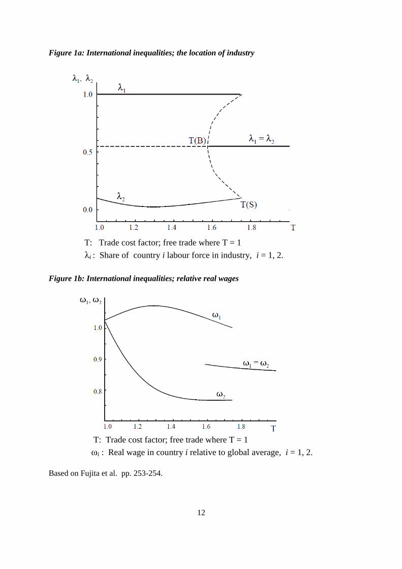
of trade costs at which bifurcation of equilibrium takes place. These are illustrated on Figure

1a, which has the share of industrial employment in each country’s labour force on the

vertical axis and trade frictions on the horizontal. At critical value T(S) two further equilibria

emerge, one with country 1 specialised in industry (λ1 = 1) and country 2 retaining a lower

level of industrial employment (1 > λ2 ≥ 0), the other symmetric (i.e. with country labels

reversed). The reason is that, as outlined above, intermediate goods create an agglomeration

force, with firms in an agglomeration benefitting from forward linkages (lots of suppliers in

the same place) and backwards linkages (lots of local intermediate demand for their output).

11

The second critical value is T(B), the point of symmetry breaking. At trade costs lower than

this the symmetric equilibrium is unstable (and therefore indicated by a dashed line). If one

country has just slightly more industry than the other then it is profitable for further firms to

move into this country, amplifying the difference between them. In the simplest model T(S)

> T(B) and in the interval between these values there are five equilibria, three of them stable

and two (the curved dashed lines) unstable.

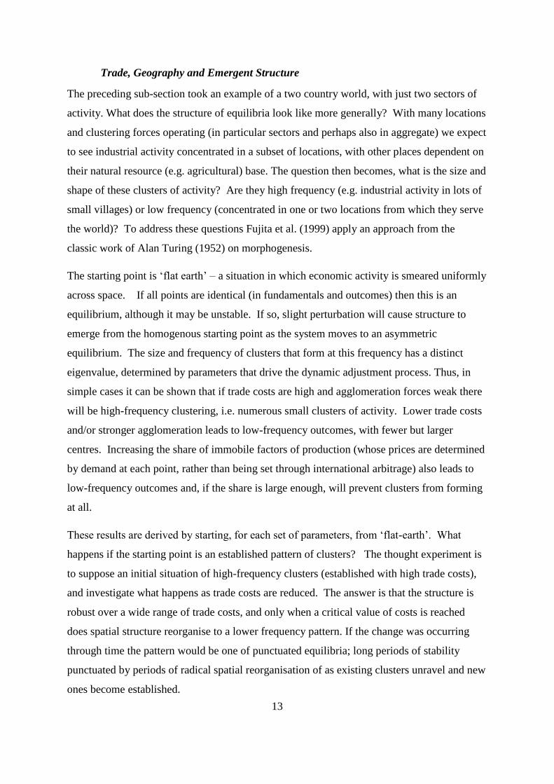
Figure 1b gives the corresponding real wages in each country, ωi, relative to world average

real wages (illustrated just for stable equilibria where country 1 has industry). Evidently,

clustering of industry in one place creates international inequalities. The divergence of

income levels reaches a maximum, beyond which further reductions in trade costs bring

convergence of incomes, although not of economic structure. The reason is that, in this

example, both the dispersion and concentration forces (mechanisms (ii) and (iii)) are assumed

to operate only via trade costs, so as these costs go to zero so too does their effect. In the

limit of perfectly free trade (T = 1) the location of industry becomes indeterminate, and all

prices and incomes are the same in both countries (factor price equalisation).

How is this picture altered if other locations mechanisms are brought into play? Other

agglomeration mechanisms (for example better labour market matching or skill development)

increase the likelihood of agglomeration and makes it less dependent on trade costs, T. Thus,

even with perfectly free trade, labour market forces might lead clusters to be persistent.

Migration (mechanism (iv)) further increases the likelihood of clustering of activity as it

tends to make large markets larger (the home market effect and core-periphery model).

Migration may also operate by creating larger pools of labour – particularly skilled labour –

in existing centres of activity. Pushing in the other direction are immobile factors, and the

fact that centres of activity will have relatively high prices of such factors. In the urban

context this is high land rents, and internationally it is high wages and labour costs.

The structure of equilibria outlined above is radically different from that of classical trade

theory, and provides alternative insights into the effects of trade. At its broadest, it gives

insight into the rise and fall of international inequalities, from the great divergence (the rise of

international inequalities following Northern Europe’s industrialisation and the

accompanying deindustrialisation of parts of Asia) through to the geographical spread of

industry that has emerged during the era of globalisation.

12

Figure 1a: International inequalities; the location of industry

Figure 1b: International inequalities; relative real wages

Based on Fujita et al. pp. 253-254.

T: Trade cost factor; free trade where T = 1

λi : Share of country i labour force in industry, i = 1, 2.

T: Trade cost factor; free trade where T = 1

ωi : Real wage in country i relative to global average, i = 1, 2.

13

Trade, Geography and Emergent Structure

The preceding sub-section took an example of a two country world, with just two sectors of

activity. What does the structure of equilibria look like more generally? With many locations

and clustering forces operating (in particular sectors and perhaps also in aggregate) we expect

to see industrial activity concentrated in a subset of locations, with other places dependent on

their natural resource (e.g. agricultural) base. The question then becomes, what is the size and

shape of these clusters of activity? Are they high frequency (e.g. industrial activity in lots of

small villages) or low frequency (concentrated in one or two locations from which they serve

the world)? To address these questions Fujita et al. (1999) apply an approach from the

classic work of Alan Turing (1952) on morphogenesis.

The starting point is ‘flat earth’ – a situation in which economic activity is smeared uniformly

across space. If all points are identical (in fundamentals and outcomes) then this is an

equilibrium, although it may be unstable. If so, slight perturbation will cause structure to

emerge from the homogenous starting point as the system moves to an asymmetric

equilibrium. The size and frequency of clusters that form at this frequency has a distinct

eigenvalue, determined by parameters that drive the dynamic adjustment process. Thus, in

simple cases it can be shown that if trade costs are high and agglomeration forces weak there

will be high-frequency clustering, i.e. numerous small clusters of activity. Lower trade costs

and/or stronger agglomeration leads to low-frequency outcomes, with fewer but larger

centres. Increasing the share of immobile factors of production (whose prices are determined

by demand at each point, rather than being set through international arbitrage) also leads to

low-frequency outcomes and, if the share is large enough, will prevent clusters from forming

at all.

These results are derived by starting, for each set of parameters, from ‘flat-earth’. What

happens if the starting point is an established pattern of clusters? The thought experiment is

to suppose an initial situation of high-frequency clusters (established with high trade costs),

and investigate what happens as trade costs are reduced. The answer is that the structure is

robust over a wide range of trade costs, and only when a critical value of costs is reached

does spatial structure reorganise to a lower frequency pattern. If the change was occurring

through time the pattern would be one of punctuated equilibria; long periods of stability

punctuated by periods of radical spatial reorganisation of as existing clusters unravel and new

ones become established.

14

The robustness of a given spatial structure derives from several forces. One is the rents of

agglomeration. An established centre has high productivity and a hence an advantage over

other places. In equilibrium the advantage is captured by immobile factors – land in the case

of cities, labour in the international context. Small changes may squeeze these rents, but not

to the point where it ceases to be profitable to operate. This argument is amplified by the fact

that capital – buildings, but also human capital in sector specific skills -- is sunk in existing

centres, so is earning quasi-rents. The other side of this coin is the difficulty of establishing

new activities in new places, this creating obstacles to economic development.

Economic Development and Coordination Failure

Agglomeration forces are generally driven by economies of scale which are external to

individual economic agents (firms or workers) but internal to a place which, depending on

context, may be a district within a city, a wider region, or a country as a whole. This

externality creates a ‘first-mover problem’ and means that it is hard to start an activity in a

new place. If a place has the activity then agglomeration benefits mean that productivity is

high enough for the place to be competitive (even at relatively high wages). If the place does

not have the activity then the productivity of a potential entrant is low, so entry is deterred.

Coordinated action by many firms could achieve scale, but coordination failure may mean

that the place remains trapped in a low-level equilibrium.

This problem is fundamental for the regeneration of areas of a city, for policy towards

lagging regions, and for structural transformation in developing economies. For example, a

developing economy may be accumulating factors of production and technology, and

acquiring a potential comparative advantage in new sectors. However, in the absence of

existing activity productivity is low, it is not profitable for any single firm to enter, and this

potential comparative advantage is not realised. This coordination failure means that

development of such sectors will commence later than is efficient and that there is scope for

policy intervention. This argument formed the basis of ‘big-push’ models of economic

development (Hirschman, 1958, Murphy and Shleifer 1989) and for policies that promote

linkages between related sectors (Myrdal 1957, Hausman and Hidalgo 2009).

For practical purposes, the sectoral scope of agglomeration effects is important. Trade

liberalisation and falling transport costs have enabled the development of global production

networks in which a particular country (or city) specialises in a narrow part of the production

15

process, sometimes referred to as ‘task specialisation’.14 Such narrowly defined tasks may

have an extreme factor intensity (e.g. be very unskilled labour intensive), so that factor cost

differentials are particularly important in location decisions. Furthermore, it is easier for

countries to achieve scale in production of narrow tasks than it is to get scale and productivity

across a whole sector or range of sectors. Thus, a development path has been to create jobs

through clusters of activity in sectors such as ready-made garments (employing 4 million

people in Bangladesh, clustered around Dhaka), electronic components or assembly.

However, global production networks have their own economic geography. They form

between countries which have both significant factor cost differences and proximity (i.e.

within East Asia and between the US and Mexico). And they are spatially uneven, as

agglomeration economies have concentrated them in particular places. Coordination failure

matters even at this fine task level, and has made it hard for new centres to become

established, as witnessed by the numerous special economic zones that have been created

around the world but which have failed to achieve this objective.

Empirical Studies

Agglomeration economies are a key mechanism in generating unevenness. There are many

studies of the effect of economic scale and density on productivity, often undertaken on city

level data, and the first raw finding is that the elasticity of productivity with respect to city

size is of the order of 0.05-0.1. Thus, a city of 5 million inhabitants typically has productivity

12-26% higher than a city of ½ million. This raw number has been refined in many

directions. 15 For example, the skill and occupational mix of the labour force varies across

cities, impacting on measured productivity. Controlling for observed measures of skill (e.g.

education) typically brings the elasticity down by about a quarter. This might only be part of

the story, as there may be sorting, meaning that people with higher innate ability (regardless

of education) are disproportionately drawn to cities. The only way to observe this is to track

individuals as they move in to cities or to cities of different sizes. Recent empirical work

doing this suggests that the pure agglomeration effect has elasticity of 0.02 – 0.04 (Combes

and Gobillon 2015). This is still a substantial number.16

Estimates can be produced by sector, and indicate that productivity effects are largest in high-

tech sectors and business services. Corresponding to this, sectoral clustering is apparent in

many sectors (ranging from financial services and films to the production of buttons).17 The

16

extent of clustering at the sectoral level has been demonstrated by authors including Ellison

and Glaeser (1997), who show that many US industries are much more clustered than would

be expected by randomness. This is linked to the home market effect by Davis and Weinstein

(2003). In a neo-classical model spatial variation in expenditure on a sector should be linked

with less than proportional variation in production, whereas in a geography model the home

market effect would cause the increase in production to be more than proportional. They find

the latter effect present in many manufacturing industries.

Finally: does geography matter for income differences? Effects are expected to show up in

the prices of immobile factors and, within countries, this is apparent in variations in the price

of land between rural and urban areas of different sizes. Internationally, several lines of

research have looked at the impact of geography on income. The impact of natural

geography is studied in a line of work following Sachs and Warner (2002), pointing to the

sometimes negative impact of natural resource and fossil fuel abundance on per capita

incomes. The impact of economic geography is studied by constructing various measures of

access to markets and to suppliers (measures derived from estimating gravity trade models)

and estimating their impact on income (Redding and Venables 2004, Head and Mayer 2011).

These measures explain a substantial proportion of cross-country variation in per capita

income, and estimated parameters are consistent with plausible values of model parameters.

Establishing that the relationship is causal is problematic, particularly as other variables such

as quality of institutions may be highly correlated with market access and income levels. In

the search to find solutions to this problem researchers have looked for natural experiments,

one notable one being the partition of Germany (Redding and Sturm 2008). West German

cities close to the border with the East experienced substantial population decline, attributed

by the authors to the loss of previous trading links and market access.18

Future Directions

Geography is now incorporated in economic models of international trade, although the focus

has been predominantly on trade costs and gravity rather than the richer story of firm

location, unevenness, and multiple equilibria. Firm location and spatial unevenness are

developed more fully in the literature on urban and regional economics where there is both

analytical and empirical work studying the location of activity and quantifying the

agglomeration forces that shape it.

17

These developments have laid the foundations for thinking about policy, but the research

literature is far from having a robust set of guidelines for formulation of spatial policy. Vast

resources are spent trying to promote the development of lagging regions – internationally,

within countries, and within cities. Much of this is done in the hope of achieving

transformational change (i.e. encouraging positive feedback mechanisms to come into play so

that an area will develop) but little is yet known about circumstances under which this is

more or less likely to occur.19 To take one example, China’s belt and road initiative is a

trillion dollar experiment in economic geography and trade; do we have the tools to think

through its likely effects? Developing such tools remains the challenge, and one route is

through the emerging literature on quantitative spatial economics in which economic

geography models are calibrated to urban or national data (Redding and Rossi-Hansburg

2017, Donaldson 2015). Effects of policy will always be context specific and, given

increasing returns and multiple equilibria, have an inherent uncertainty. Prediction may not

be possible, but quantitative tools firmly grounded in theory and data will provide a way of

illustrating scenarios of possible outcomes.

18

References

Allen, T. and C. Arkolakis (2014). ‘Trade and the topography of the spatial economy’, The

Quarterly Journal of Economics, 129 (3), 1085–1139.

Anderson, J. (2011). ‘The Gravity Model’, The Annual Review of Economics 3 (1), 133–160.

Armington, P. (1969) "A Theory of Demand for Products Distinguished by Place of

Production", International Monetary Fund Staff Papers, XVI 159-78

Baldwin, R.E., Forslid, R., Martin, P., Ottaviano, G. & Robert-Nicoud, F. (2003). Economic

Geography and Public Policy, Princeton University Press, Princeton NJ.

Baldwin, R. (2016). The great convergence; information technology and the new

globalization, Harvard University Press, Cambridge MA

Behrens, K., A.R. Lamorgese, G. Ottaviano, & T. Tabuchi, (2009). ‘Beyond the home market

effect: Market size and specialization in a multi-country world’, Journal of

International Economics, 79(2), pages 259-265.

Brakman, S., H. Garretsen & C. van Marrewijk (2001). An introduction to Geographical

Economics, Cambridge University Press, Cambridge UK

Cairncross, F., (1997) The Death of Distance: How the Communications Revolution will

change our Lives, London, U.K.: Orion Business Books.

Combes, P. & L. Gobillon (2015). ‘Empirics of agglomeration economies’, in: G. Duranton,

J. V. Henderson & W. Strange (eds.), Handbook of Regional and Urban Economics,

vol. 5, 247-348, North-Holland, Amsterdam.

Davis, D.R. & D.E. Weinstein (2003). ‘Market access, economic geography and comparative

advantage; an empirical test’, Journal of International Economics, 59; 1-23.

Disdier, A.C. & K. Head (2008). ‘The puzzling persistence of the distance effect on bilateral

trade’. The Review of Economics and statistics, 90(1), 37-48.

Dixit, A. K. & J. E. Stiglitz (1977), ‘Monopolistic competition and optimum product

diversity’, American Economic Review, 67:297-308

Donaldson, D. (2015) ‘The gains from market integration’, Annual Review of Economics, 7;

619-47.

Duranton, G. & D. Puga (2004). ‘Micro-foundations of urban agglomeration economies’, in:

J. V. Henderson & J. F. Thisse (eds.), Handbook of Regional and Urban Economics,

volume 4, chapter 48, pages 2063-2117, Elsevier.

Duranton, G. & A.J. Venables (2018). ‘Place-based policies for development’, World Bank

Policy Research Working paper 8410, CEPR discussion paper 12889.

Eaton, J. and S. Kortum (2002). ‘Technology, Geography and Trade’, Econometrica, 70(5)

1741-1779.

Fujita, M., P.R. Krugman & A.J. Venables, (1999). The Spatial Economy: Cities, Regions,

and International Trade. MIT Press, Cambridge, MA.

19

Fujita, M. & J.F. Thisse (2002) The Economics of Agglomeration, Cambridge University

Press, Cambridge

Grossman, G.M. and E. Rossi-Hansberg (2008). ‘Trading tasks: a simple theory of

offshoring’, American Economic Review, 98(5) 1978-97.

Hausmann, R. & C.A. Hidalgo (2009) ‘The building blocks of economic complexity’

Proceedings of the National Academy of Sciences, 106 (26), 10570-75

Head, K. & T. Mayer, (2004). ‘The empirics of agglomeration and trade’. Handbook of

regional and urban economics 4, 2609–2669.

Head, K. & T. Mayer, (2011). ‘Gravity, market potential and economic development’ Journal

of Economic Geography. 11 (2), 281-294.

Head, K., & T. Mayer, (2014), ‘Gravity Equations: Workhorse,Toolkit, and Cookbook’, in

Gopinath, G, E. Helpman and K. Rogoff (eds), Handbook of International Economics,

vol. 4, 131-195, Elsevier:

Head, K., T. Mayer & J. Ries (2009). ‘How remote is the offshoring threat?’. European

Economic Review, 53(1): 429-444.

Helpman, E. and P. Krugman (1985) Market Structure and Foreign Trade. Cambridge, MA:

MIT Press.

Hirschman, A.O. (1958) The Strategy of Economic Development, New Haven CT, Yale

University Press.

Kline, P., and E. Moretti. (2013). ‘Local economic development, agglomeration economies,

and the big push: 100 years of evidence from the Tennessee Valley Authority’.

Quarterly Journal of Economics 129(1): 275-331.

Krugman, P.R. (1991) ‘Increasing returns and economic geography’, Journal of Political

Economy, 99(3), 483-499.

Krugman, P. R. (1991b). Geography and trade. Cambridge (Mass.): MIT Press.

Krugman, P.R., M. Obstfeld & M. Melitz (2015) International Economics; theory and policy,

Pearson

Lendle, A., M. Olarreaga, S. Schropp & P.-L. Vézina, (2016) "There Goes Gravity: eBay

and the Death of Distance," Economic Journal, 126 (591), 406-441.

Markusen J. R. (2002) Multinational Firms and the Theory of International Trade,

Cambridge: MIT Press.

Marshall, A. (1920) Principles of Economics, London, Macmillan (8th edn.)

Melitz, M. & S.J. Redding (2014) ‘Heterogeneous Firms and Trade’ in Gopinath, G, E.

Helpman & K. Rogoff (eds), Handbook of International Economics, Vol. 4 Elsevier:

North Holland, 1-54, 2014.

Moretti, E. (2013) The New Geography of Jobs, Mariner Books, New York.

Murphy, K.M., A. Shleifer & R.W. Vishny (1989), ‘Income distribution, market size, and

industrialisation’, Quarterly Journal of Economics, 104: 537-64

20

Myrdal, G. (1957) ‘Economic Theory and under-developed regions’ London, Duckworth

Norman, V. & A.J. Venables (1995) ‘International trade, factor mobility and trade costs’

Economic Journal 105(433), 1488-1504.

Redding, S.J. & M. Turner (2015) "Transportation Costs and the Spatial Organization of

Economic Activity" in (eds) Gilles Duranton, J. Vernon Henderson and William

Strange, Handbook of Urban and Regional Economics, 1339-1398, 2015.

Redding, S.J, & E. Rossi-Hansburg (2017) ‘Quantitative Spatial Economics’ Annual Review

of Economics. 9 (1), 21-58.

Redding, S.J, & A.J. Venables (2004) ‘Economic Geography and International Inequality,’

Journal of International Economics. 62 (1), 53-82.

Rosenthal S. & W. Strange. (2004). ‘Evidence on the nature and sources of agglomeration

economies’ in V. Henderson & J-F. Thisse (eds) Handbook of Regional and Urban

Economics,vol 4, pp 2119-2171. North-Holland, Amsterdam

Sachs, J.D. & A.M. Warner (2001) ‘The curse of natural resources’, European Economic

Review, 45(4): 827-838

Tinbergen, J. (1962) Shaping the world economy; suggestions for an international economic

policy, New York, Twentieth Century Fund.

Turing, A. (1952) ‘The chemical basis of morphogenesis’ Philosophical Transactions of the

Royal Society of London, 237: 37-72.

Venables, A. J. (1996) ‘Equilibrium locations of vertically linked industries’, International

Economic Review, 37, 341-359.

Further Reading

Accessible introductions to the area are Krugman (1991b), Moretti (2013). A textbook

treatment is given by Brakman, et al. (2001). There are good surveys of a number of aspects

of the literature, including Donaldson (2015) , Duranton & Puga (2004), Head & Mayer,

(2004), (2015), Redding & Rossi-Hansburg (2017) . A comprehensive statement of early

development of the field is Fujita et al. (1999).

21

Notes 1 There are also distinct literatures on frictions due to trade policy and on the effects of factor

mobility. See Norman and Venables (1995) for a synthesis of trade frictions and factor mobility in a

Heckscher-Ohlin framework.

2 Trade can be generated by national level product differentiation (Armington 1969), Ricardian

productivity differences in a multi-commodity setting (Eaton and Kortum 2002), or factor

endowments with firm level product differentiation (Helpman and Krugman 1985).

3 Nineteenth century ‘social physics’ hypothesised that human interactions were analogous to

physical ones. Physical gravity operates in 3-dimensional space so distance has coefficient -2. The

surface of the earth is 2-dimensional, so the analogous gravity coefficient would be expected to be -1.

4 The terminology follows Redding and Venables (2004). The familiar concept of country i market

access is an inverse distance weighted sum of market capacities across countries j with which i trades,

market accessi = j ijj dm / . See also Anderson (2011) for links with the gravity model.

5 The benchmark model sketched here assumes that all firms in a particular country/ industry are

symmetric. If firms are heterogeneous, e.g. in their productivity levels, then the marginal firm breaks

even and firms with higher productivities make positive profits. For development of such models see

Melitz and Redding (2014).

6 In a particular sector of a closed economy there is just one equation and a single variable 1n . In a

multi-country context i, j are values of an index over the total number of countries so that equation (2)

is a simultaneous system determining the number of firms active in each country. Solution is subject

to the impossibility of a negative number of firms, so 0 in , 0in , complementary slack.

7 In the Dixit-Stiglitz framework the measure of market crowdedness is the price index of all varieties

sold in the country j market.

8 For generalisation of the home market effect to many countries and industries see Behrens et al.

(2009).

9 Discussion dates back to at least Alfred Marshall (Marshall 1920). For a modern survey see

Duranton and Puga (2004).

10 The supplier will capture the full benefit only if able to perfectly price discriminate. Otherwise, the

customer will also receive some consumer/ user surplus on the introduction of a new product. This

observation is central to the wide-range of economic models in which the number and variety of

goods and services offered is endogenous (following Dixit and Stiglitz 1977).

11 For an elegant synthesis of the tension between dispersion and agglomeration forces and an

application to intra-country unevenness see Allen and Arkolakis (2014).

12 This section draws on Venables (1996), see also Fujita et al. (1999).

13 In general this would be through a full input-output matrix. In this example it is aggregated to a

single sector using some of its own (differentiated) outputs as inputs.

14 See Grossman and Rossi-Hansburg (2008) and, for a wider view of global production networks,

Baldwin (2016).

15 See Rosenthal and Strange (2004) for a survey.

16 In some contexts, it may not be appropriate to impose all these controls. Suppose that someone

achieves high productivity by undertaking education to acquire a skill that is in demand only in large

22

cities. Then both the city and the education are necessary for attaining the productivity, and it would

be wrong to attribute it all to education.

17 The city of Qiaotou produces 60% of the world’s buttons and 200,000km of zippers per year.

18 There are substantial recent literatures re-evaluating the gains from trade and looking at the effects

of transport improvements. These are outside the scope of this paper, and are both surveyed in

Donaldson (2015).

19 An exception is the careful study of the Tennessee Valley Authority by Kline and Moretti (2013).

See Duranton and Venables (2018) for further discussion of issues and a review of some of this

literature.