Embed Size (px)
Citation preview
Information and Computation 219 (2012) 39–57
Contents lists available at SciVerse ScienceDirect
Information and Computation
www.elsevier.com/locate/yinco
Efficient algorithms for the conditional covering problem
Robert Benkoczi a, Binay Bhattacharya b,1, Yuzhuang Hu b, Chien-Hsin Lin c, Qiaosheng Shi b,Biing-Feng Wang c,∗,2
a Mathematics and Computer Science, University of Lethbridge, Lethbridge AB T1K3M4, Canadab School of Computing Science, Simon Fraser University, Burnaby, BC, V5A 1S6, Canadac Department of Computer Science, National Tsing Hua University, Hsinchu, 30043, Taiwan, ROC
a r t i c l e i n f o a b s t r a c t
Article history:Received 16 March 2011Revised 20 December 2011Available online 3 September 2012
Keywords:AlgorithmsGraphsCovering location problemsConditional coveringDynamic programming
We consider the conditional covering problem in an undirected network, in which eachvertex represents a demand point that must be covered by a facility as well as a potentialfacility site. Each facility can cover all vertices within a given coverage radius, except thevertex at which the facility is located. The objective is to locate facilities to cover allvertices such that the total facility location cost is minimized. In this paper, new upperbounds are proposed for the conditional covering problem on paths, cycles, extended stars,and trees. In particular, we provide an O (n log n)-time algorithm for paths, an O (n2 log n)-time algorithm for cycles, an O (n1.5 log n)-time algorithm for extended stars, and an O (n3)-time algorithm for trees. Our algorithms for paths, extended stars, and trees improve theprevious upper bounds from O (n2), O (n2), and O (n4), respectively.
© 2012 Elsevier Inc. All rights reserved.
1. Introduction
Over three decades, covering location problems on networks have received much attention from researchers in the fieldsof transportation and communication. One of the classical problems is the location set covering problem (for short, LSCP) [21].Given a set of demand points and a set of potential facility sites, the problem is to determine the minimum number offacility sites so that each given demand point is covered by at least one facility. The set of demand points and the set offacility sites may be identical, or partially overlapping or disjoint. Due to practical considerations, numerous extensions ofthe LSCP have been defined and studied [18]. A useful extension is the conditional covering problem (for short, CCP) [4,12].The CCP has the same objective as the LSCP but with an additional constraint: each selected facility site must be coveredby at least one other selected site. It is easy to motivate the inter-facility support imposed by the CCP in many practicalapplications, such as locating facilities in distribution systems, emergency systems, and communication systems [12]. Forexample, consider the deployment of distributors that have non-overlapping services regions. The inter-facility support isuseful in order to offset shortages of a distributor by a nearby distributor promptly.
The CCP was firstly introduced by Moon and Chaudhry [12]. They gave an integer linear programming model for theproblem and then approached its solution by linear relaxation and cutting plane techniques. Moon and Chaudhry’s com-putational results were disappointing. However, their study provided deep insight into the problem and stimulated furtherresearch on the CCP. Efficient heuristics algorithms for the CCP had been extensively studied in [3,4,9,11]. Moon and Pa-payanopoulos [13] studied the CCP on a tree, in which the set of vertices represents the set of demand points and the set of
* Corresponding author. Fax: +886 3 5723694.E-mail addresses: [email protected] (R. Benkoczi), [email protected] (B. Bhattacharya), [email protected] (Y. Hu), [email protected]
(C.-H. Lin), [email protected] (Q. Shi), [email protected] (B.-F. Wang).1 Research was partially supported by MITACS and NSERC.2 Research was supported by the National Science Council of the Republic of China under grant NSC-100-2221-E-007-070-MY3.
0890-5401/$ – see front matter © 2012 Elsevier Inc. All rights reserved.http://dx.doi.org/10.1016/j.ic.2012.08.003
40 R. Benkoczi et al. / Information and Computation 219 (2012) 39–57
all points on the edges represents the set of potential facility sites. They had a linear-time algorithm for the CCP on a tree.Lunday, Smith, and Goldberg [10] introduced a modified version of the CCP, which is defined as follows. Let G = (V , E) be agraph, where V is the vertex set and E is the edge set. The vertex set V represents the set of demand points as well as theset of potential facility sites. A facility located at a vertex i ∈ V incurs a non-negative cost ci and provides a non-negativecoverage radius Ri . Each edge e ∈ E is associated with a non-negative length. Let d(i, j) denote the length of a shortestpath in G from i to j, where i, j ∈ V . A vertex i ∈ V is covered by a vertex j ∈ V if i �= j and d(i, j) � R j . In other words,a facility located at a vertex covers all vertices within its coverage radius, except for the vertex at which it is located. Themodified version of the CCP seeks to minimize the sum of open-facility costs required to cover all vertices in G , i.e.,
min∑i∈V
cixi s.t.
xi ∈ {0,1} for i ∈ V ;for i ∈ V , ∃ j ∈ V ( j �= i) ∧ (x j = 1) ∧ (
d(i, j) � R j).
There are two differences between the modified version and the original CCP. First, in the original CCP, each demandpoint is specified with a distance constraint and a demand point is covered by a facility only if the facility is locatedwithin its distance constraint. Second, in the original CCP, the set of demand points and the set of potential facility sitesmay be different. This modified version arises in several military and security applications that are becoming increasinglyimportant [10].
Lunday, Smith, and Goldberg’s modified version is a natural variant of the CCP. Moon and Chaudhry’s integer linearprogramming model [12] as well as the heuristics algorithms in [3,4,9,11] are applicable to their modified version. Thismodified version is the focus of this paper. For convenience, in the remainder of this paper, this modified version is simplyreferred as the MCCP. The total dominating set problem, introduced by Cockayne, Dawes, and Hedetniemi [5], is a specialcase of the MCCP, in which all edge lengths, coverage radii, and costs are 1. The total dominating set problem is stronglyNP-hard [14]. Therefore, the MCCP is also strongly NP-hard. In several special cases, polynomial-time algorithms are knownfor the total dominating set problem and the MCCP. Let n = |V |. For the total dominating set problem, Pfaff, Laskar, andHedetniemi [15] had an O (n)-time algorithm for series-parallel graphs, Laskar et al. [8] had an O (n)-time algorithm fortrees, Bertossi and Gori [1] had an O (n log n)-time algorithm for interval graphs, and Chang [2] had an O (n log logn)-time algorithm for interval graphs with endpoints sorted. Lunday, Smith, and Goldberg [10] studied the MCCP on a path,motivated by some military applications. They gave an O (n2)-time algorithm for the special case that all coverage radii areuniform, and an O (n)-time algorithm for the special case that all coverage radii and all location costs are uniform. Later,Horne and Smith [6] gave an O (n2)-time algorithm for the MCCP on a path, with non-uniform coverage radii and locationcosts. In the same paper, using their path algorithm as a procedure, they also derived an O (n2)-time algorithm for the MCCPon an extended star, which is a rooted tree consisting of one or more paths, all incident to the root. Very recently, Sivan,Harini, and Rangan [20] found that Horne and Smith’s path algorithm has a bug and gave a correct O (n3)-time algorithm.Actually, as indicated in [19], the bug can be easily rectified without increasing the time complexity. For the MCCP on atree, Horne and Smith [7] had an O (n4)-time algorithm. For the MCCP on an interval graph, Sivan, Harini, and Rangan [20]had an O (n2)-time algorithm for the special case that all edge lengths and costs are uniform. Rana, Pal, and Pal [17] hadan O (n)-time algorithm for the special case that all edge lengths and costs are 1, and all coverage radii are the same andlarger than 1.
In this paper, efficient algorithms are proposed for the MCCP on paths, cycles, extended stars, and trees. In particular, weprovide an O (n log n)-time algorithm for paths, an O (n2 logn)-time algorithm for cycles, an O (n1.5 log n)-time algorithm forextended stars, and an O (n3)-time algorithm for trees. The proposed algorithms improve the previous upper bounds in [6,7]from O (n2), O (n2), and O (n4), respectively. Table 1 summarizes the above results on the MCCP.
The remainder of this paper is organized as follows. Section 2 presents our algorithm for paths and gives a simpleextension to cycles. Sections 3 and 4 present, respectively, our algorithms for extended stars and trees. Finally, Section 5concludes this paper.
2. Path networks
In this section, we study the MCCP on a path graph, in which the vertex set is V = {1,2, . . . ,n} and the edge set isE = {(1,2), (2,3), . . . , (n − 1,n)}. Horne and Smith [6] had an O (n2)-time algorithm for the MCCP on a path. As indicatedin [19], their algorithm has a small bug. In Section 2.1, we first present an O (n2)-time algorithm, which is a revision of thealgorithm in [6]. Then, in Section 2.2, we show how to modify the algorithm in Section 2.1 so as to solve the MCCP problemon a path in O (n log n) time. In Section 2.3, we give a simple extension of our path algorithm to cycles.
2.1. An O (n2)-time algorithm
For each i ∈ V , the lower reach of i is h(i) = min{ j | j ∈ V , d(i, j) � Ri}, and the upper reach of i is g(i) = max{ j | j ∈ V ,
d(i, j) � Ri}. A vertex i ∈ V dominates another vertex j ∈ V if [h( j), g( j)] ⊂ [h(i), g(i)]. For each i ∈ V , let D(i) be the setof vertices dominated by i. Let U be the sequence obtained by ordering the vertices in V by the following rule: a vertex j
R. Benkoczi et al. / Information and Computation 219 (2012) 39–57 41
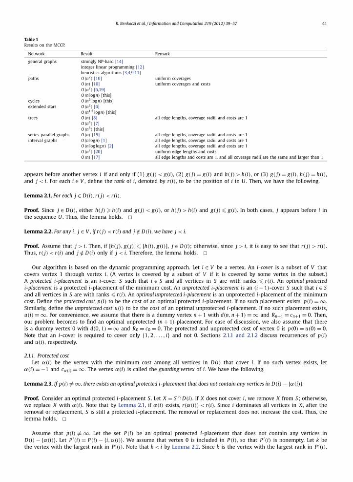
Table 1Results on the MCCP.
Network Result Remark
general graphs strongly NP-hard [14]integer linear programming [12]heuristics algorithms [3,4,9,11]
paths O (n2) [10] uniform coveragesO (n) [10] uniform coverages and costsO (n2) [6,19]O (n logn) [this]
cycles O (n2 log n) [this]extended stars O (n2) [6]
O (n1.5 logn) [this]trees O (n) [8] all edge lengths, coverage radii, and costs are 1
O (n4) [7]O (n3) [this]
series-parallel graphs O (n) [15] all edge lengths, coverage radii, and costs are 1interval graphs O (n logn) [1] all edge lengths, coverage radii, and costs are 1
O (n log logn) [2] all edge lengths, coverage radii, and costs are 1O (n2) [20] uniform edge lengths and costsO (n) [17] all edge lengths and costs are 1, and all coverage radii are the same and larger than 1
appears before another vertex i if and only if (1) g( j) < g(i), (2) g( j) = g(i) and h( j) > h(i), or (3) g( j) = g(i), h( j) = h(i),and j < i. For each i ∈ V , define the rank of i, denoted by r(i), to be the position of i in U . Then, we have the following.
Lemma 2.1. For each j ∈ D(i), r( j) < r(i).
Proof. Since j ∈ D(i), either h( j) � h(i) and g( j) < g(i), or h( j) > h(i) and g( j) � g(i). In both cases, j appears before i inthe sequence U . Thus, the lemma holds. �Lemma 2.2. For any i, j ∈ V , if r( j) < r(i) and j /∈ D(i), we have j < i.
Proof. Assume that j > i. Then, if [h( j), g( j)] ⊂ [h(i), g(i)], j ∈ D(i); otherwise, since j > i, it is easy to see that r( j) > r(i).Thus, r( j) < r(i) and j /∈ D(i) only if j < i. Therefore, the lemma holds. �
Our algorithm is based on the dynamic programming approach. Let i ∈ V be a vertex. An i-cover is a subset of V thatcovers vertex 1 through vertex i. (A vertex is covered by a subset of V if it is covered by some vertex in the subset.)A protected i-placement is an i-cover S such that i ∈ S and all vertices in S are with ranks � r(i). An optimal protectedi-placement is a protected i-placement of the minimum cost. An unprotected i-placement is an (i − 1)-cover S such that i ∈ Sand all vertices in S are with ranks � r(i). An optimal unprotected i-placement is an unprotected i-placement of the minimumcost. Define the protected cost p(i) to be the cost of an optimal protected i-placement. If no such placement exists, p(i) = ∞.Similarly, define the unprotected cost u(i) to be the cost of an optimal unprotected i-placement. If no such placement exists,u(i) = ∞. For convenience, we assume that there is a dummy vertex n + 1 with d(n,n + 1) = ∞ and Rn+1 = cn+1 = 0. Then,our problem becomes to find an optimal unprotected (n + 1)-placement. For ease of discussion, we also assume that thereis a dummy vertex 0 with d(0,1) = ∞ and R0 = c0 = 0. The protected and unprotected cost of vertex 0 is p(0) = u(0) = 0.Note that an i-cover is required to cover only {1,2, . . . , i} and not 0. Sections 2.1.1 and 2.1.2 discuss recurrences of p(i)and u(i), respectively.
2.1.1. Protected costLet α(i) be the vertex with the minimum cost among all vertices in D(i) that cover i. If no such vertex exists, let
α(i) = −1 and cα(i) = ∞. The vertex α(i) is called the guarding vertex of i. We have the following.
Lemma 2.3. If p(i) �= ∞, there exists an optimal protected i-placement that does not contain any vertices in D(i) − {α(i)}.
Proof. Consider an optimal protected i-placement S . Let X = S ∩ D(i). If X does not cover i, we remove X from S; otherwise,we replace X with α(i). Note that by Lemma 2.1, if α(i) exists, r(α(i)) < r(i). Since i dominates all vertices in X , after theremoval or replacement, S is still a protected i-placement. The removal or replacement does not increase the cost. Thus, thelemma holds. �
Assume that p(i) �= ∞. Let the set P (i) be an optimal protected i-placement that does not contain any vertices inD(i) − {α(i)}. Let P ′(i) = P (i) − {i,α(i)}. We assume that vertex 0 is included in P (i), so that P ′(i) is nonempty. Let k bethe vertex with the largest rank in P ′(i). Note that k < i by Lemma 2.2. Since k is the vertex with the largest rank in P ′(i),
42 R. Benkoczi et al. / Information and Computation 219 (2012) 39–57
no vertex in P ′(i) has an upper reach larger than g(k). Thus, P ′(i) covers i if and only if k covers i, from which we concludethat α(i) ∈ P (i) if k does not cover i. On the other hand, if k covers i, α(i) /∈ P (i); otherwise, we can remove α(i) to reducethe cost. Therefore, we have the following.
Lemma 2.4. k covers i if and only if α(i) /∈ P (i).
Lemma 2.5. {k, i} covers vertices k + 1,k + 2, . . . , i − 1.
Proof. No vertex in P ′(i) has an upper reach larger than g(k). Since α(i) ∈ D(i), the lower reach of α(i) is not smallerthan h(i). Thus, if a vertex between k and i is not covered by {k, i}, it is also not covered by P (i). Since P (i) covers allvertices between k and i, the lemma holds. �Lemma 2.6. P ′(i) covers vertices 1,2, . . . ,k − 1.
Proof. Since k < i and k /∈ D(i), we have h(k) � h(i). Thus, {i,α(i)} does not cover vertices 1,2, . . . ,h(k)− 1, from which weconclude that P ′(i) covers 1,2, . . . ,h(k) − 1. Moreover, since k ∈ P ′(i), P ′(i) also covers h(k),h(k) + 1, . . . ,k − 1. Therefore,the lemma holds. �
The following lemma describes the optimal substructure of P (i).
Lemma 2.7. If k is not covered by i, P ′(i) is an optimal protected k-placement; otherwise, P ′(i) is an optimal unprotected k-placement.
Proof. We only prove the case that k is not covered by i. The proof for the other case is similar. Assume that k is notcovered by i. By Lemma 2.6, P ′(i) covers 1,2, . . . ,k − 1. Since k is not covered by i, P ′(i) also covers k; otherwise P (i)is not an i-cover. The vertex with the largest rank in P ′(i) is k. Thus, P ′(i) is a protected k-placement. For any subsetS ⊆ V , define the cost of S to be c(S) = ∑
i∈S{ci}. Consider an optimal protected k-placement S . By Lemma 2.5, {k, i}covers k + 1,k + 2, . . . , i − 1. If k also covers i, S ∪ {i} is a protected i-placement; otherwise, by Lemma 2.4 α(i) ∈ P (i) andS ∪ {i,α(i)} is a protected i-placement. Therefore, by replacing P ′(i) with S , we can obtain from P (i) another protectedi-placement with cost c(P (i)) − c(P ′(i)) + c(S), from which we conclude that P ′(i) is an optimal protected k-placement;otherwise P (i) is also not an optimal protected i-placement. Therefore, the lemma holds. �
The set C(i) = {k | k ∈ V , r(k) < r(i), k /∈ D(i)} contains all possible candidates for k. We partition it into the followingsubsets:
K1(i) = {k | k ∈ C(i), g(k) � i, k � h(i)}, which contains the vertices that cover i and are covered by i;K2(i) = {k | k ∈ C(i), g(k) < i, k � h(i)}, which contains the vertices that do not cover i, but are covered by i;K3(i) = {k | k ∈ C(i), g(k) � i, k < h(i)}, which contains the vertices that cover i, but are not covered by i;K4(i) = {k | k ∈ C(i), g(k) < i, k < h(i), g(k) + 1 � h(i)}, which contains the vertices k such that k and i do not cover eachother, but {k, i} covers all vertices between k and i; andK5(i) = {k | k ∈ C(i), i > g(k), k < h(i), g(k) + 1 < h(i)}, which contains the vertices k such that k and i do not cover eachother, and {k, i} does not cover all vertices between k and i.
Based on Lemmas 2.4, 2.5, and 2.7, we proceed to derive a recurrence for p(i). The following cases are discussed.
Case 1: k ∈ K1(i). In this case, α(i) /∈ P (i) and P ′(i) is an optimal unprotected k-placement. Thus, p(i) = u(k) + ci .Case 2: k ∈ K2(i). In this case, α(i) ∈ P (i) and P ′(i) is an optimal unprotected k-placement. Thus, p(i) = u(k) + ci + cα(i) .Case 3: k ∈ K3(i). In this case, α(i) /∈ P (i) and P ′(i) is an optimal protected k-placement. Thus, p(i) = p(k) + ci .Case 4: k ∈ K4(i). In this case, α(i) ∈ P (i) and P ′(i) is an optimal protected k-placement. Thus, p(i) = p(k) + ci + cα(i) .Case 5: k ∈ K5(i). By Lemma 2.5, this case does not exist.Case 6: k does not exist. In this case, there does not exist any protected i-placement. Thus, p(i) = ∞.
For convenience, throughout this paper, we assume that the minimum of an empty set is ∞. Based on the abovediscussion, we obtain the following: for each i � 1,
(R1) p(i) = min{
mink∈K1(i)
u(k), mink∈K2(i)
u(k) + cα(i), mink∈K3(i)
p(k), mink∈K4(i)
p(k) + cα(i)
}+ ci .
2.1.2. Unprotected costAssume that u(i) �= ∞. Let U (i) be an optimal unprotected i-placement. Let U ′(i) = U (i) − {i}. Since i dominates all
vertices in D(i), U (i) does not contain any vertices in D(i). Let k be the vertex with the largest rank in U ′(i). Then, similarto Lemma 2.7, we can prove the following.
R. Benkoczi et al. / Information and Computation 219 (2012) 39–57 43
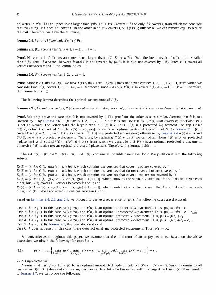
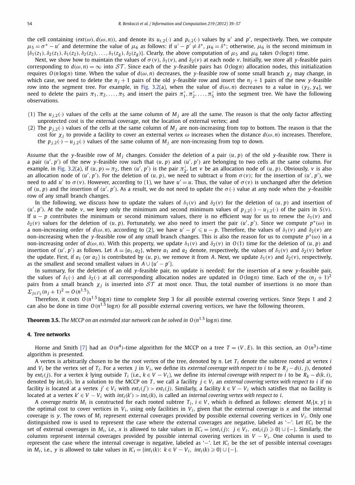
Fig. 2.1. An example.
Lemma 2.8. If k is not covered by i, U ′(i) is an optimal protected k-placement; otherwise, U ′(i) is an optimal unprotected k-placement.
Based on Lemma 2.8, we obtain the following: for each i � 1,
(R2) u(i) = min{
mink∈K1(i)∪K2(i)
u(k), mink∈K3(i)∪K4(i)
p(k)}
+ ci .
Fig. 2.1 gives an example of n = 5. Assume that p(i) and u(i) are computed for all i = 1,2, . . . ,5. Then, for the vertex 6,by definition, we have K1(6) = K2(6) = K3(6) = ∅ and K4(6) = {4,5}. Thus, p(6) = min{p(4), p(5)} + c6 + cα(6) = ∞, andu(6) = min{p(4), p(5)} + c6 = 4. In this example, {3, 4} is an optimal unprotected 6-placement.
As mentioned, our problem is to find an optimal unprotected (n + 1)-placement. Based on recurrences (R1) and (R2), itis easy to compute the value of u(n + 1) and then determine an optimal unprotected (n + 1)-placement in O (n2) time. Wehave the following.
Theorem 2.9. The MCCP on a path can be solved in O (n2) time.
2.2. An improved algorithm
In this section, we show how to modify the algorithm in Section 2.1, so as to solve the MCCP on a path in O (n log n)
time. According to recurrences (R1) and (R2), there are two difficulties in the computation of each p(i) and u(i). First, weneed to find cα(i) . Second, we need to determine the minimum values min{u(k) | k ∈ K1(i)}, min{u(k) | k ∈ K2(i)}, min{p(k) |k ∈ K3(i)}, and min{p(k) | k ∈ K4(i)}. In Section 2.2.1, we show that the finding of cα(i) can be avoided by slightly modifyingthe recurrences. In Section 2.2.2, we give further modifications to the recurrences, so that the minimum values required tocompute each p(i) and u(i) can be obtained efficiently by maintaining dynamic data structures for one-dimensional rangeminimum queries. Then, based upon the modified recurrences, we present an O (n log n)-time algorithm in Section 2.2.3.
2.2.1. Replacement of guarding verticesIn this section, we show that the finding of cα(i) can be avoided by slightly modifying (R1) and (R2). For ease of discus-
sion, we define a directed acyclic graph H corresponding to (R1) and (R2) as follows:
(1) the vertex set is V (H) = {s = u0 = p0, p1, u1, p2, u2, . . . , pn+1, un+1};(2) the edge set is E(H) = E1 ∪ E2 ∪ E3 ∪ E4 ∪ E5 ∪ E6, where E1 = {(uk, pi) | 1 � i � n + 1, k ∈ K1(i)}, E2 = {(uk, pi) | 1 �
i � n + 1, k ∈ K2(i)}, E3 = {(pk, pi) | 1 � i � n + 1, k ∈ K3(i)}, E4 = {(pk, pi) | 1 � i � n + 1, k ∈ K4(i)}, E5 = {(uk, ui) |1 � i � n + 1, k ∈ K1(i) ∪ K2(i)}, and E6 = {(pk, ui) | 1 � i � n + 1, k ∈ K3(i) ∪ K4(i)}; and
(3) all edges (uk, pi) ∈ E1, (pk, pi) ∈ E3, (uk, ui) ∈ E5, (pk, ui) ∈ E6 have length ci , and all edges (uk, pi) ∈ E2 and (pk, pi) ∈E4 have length ci + cα(i) .
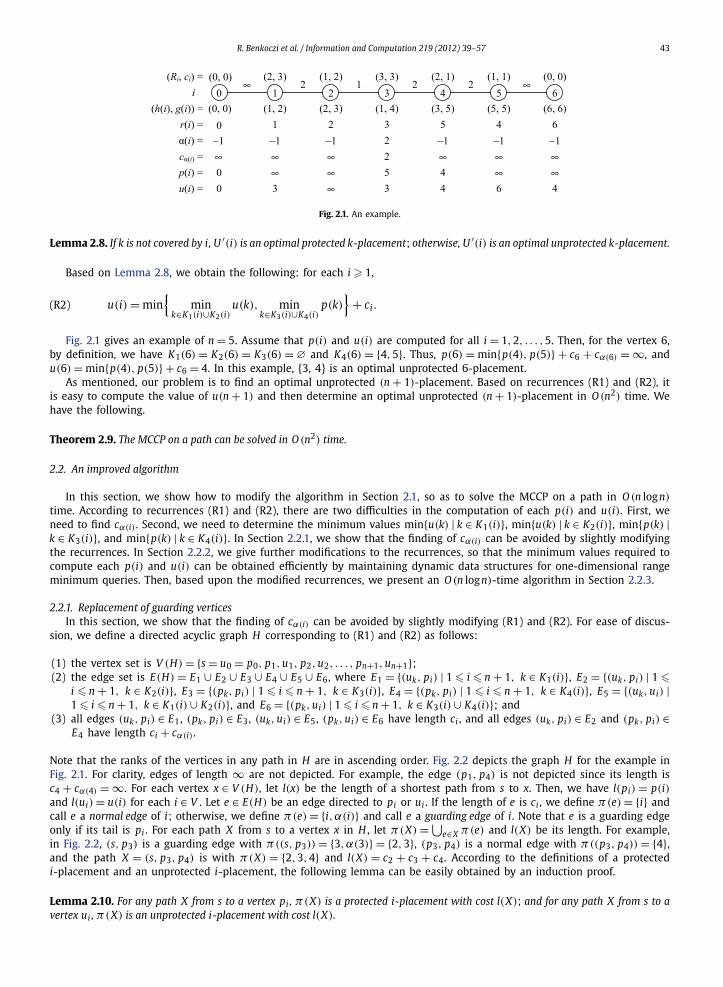
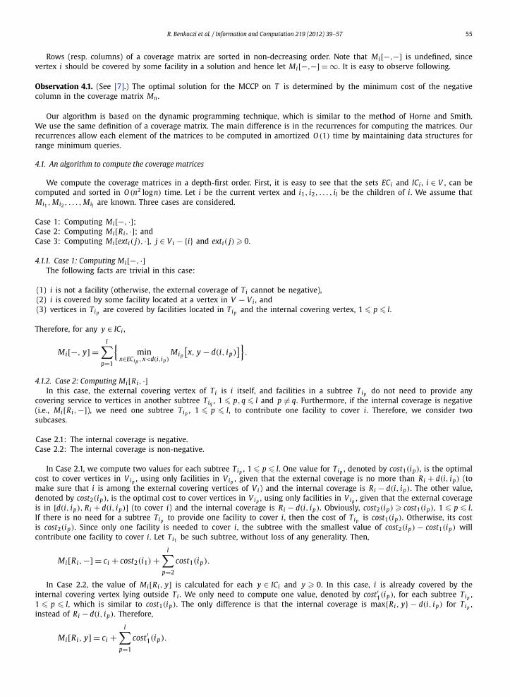
Note that the ranks of the vertices in any path in H are in ascending order. Fig. 2.2 depicts the graph H for the example inFig. 2.1. For clarity, edges of length ∞ are not depicted. For example, the edge (p1, p4) is not depicted since its length isc4 + cα(4) = ∞. For each vertex x ∈ V (H), let l(x) be the length of a shortest path from s to x. Then, we have l(pi) = p(i)and l(ui) = u(i) for each i ∈ V . Let e ∈ E(H) be an edge directed to pi or ui . If the length of e is ci , we define π(e) = {i} andcall e a normal edge of i; otherwise, we define π(e) = {i,α(i)} and call e a guarding edge of i. Note that e is a guarding edgeonly if its tail is pi . For each path X from s to a vertex x in H , let π(X) = ⋃
e∈X π(e) and l(X) be its length. For example,in Fig. 2.2, (s, p3) is a guarding edge with π((s, p3)) = {3,α(3)} = {2,3}, (p3, p4) is a normal edge with π((p3, p4)) = {4},and the path X = (s, p3, p4) is with π(X) = {2,3,4} and l(X) = c2 + c3 + c4. According to the definitions of a protectedi-placement and an unprotected i-placement, the following lemma can be easily obtained by an induction proof.
Lemma 2.10. For any path X from s to a vertex pi , π(X) is a protected i-placement with cost l(X); and for any path X from s to avertex ui , π(X) is an unprotected i-placement with cost l(X).
44 R. Benkoczi et al. / Information and Computation 219 (2012) 39–57
Fig. 2.2. The graph H . (Edges of length ∞ are omitted.)
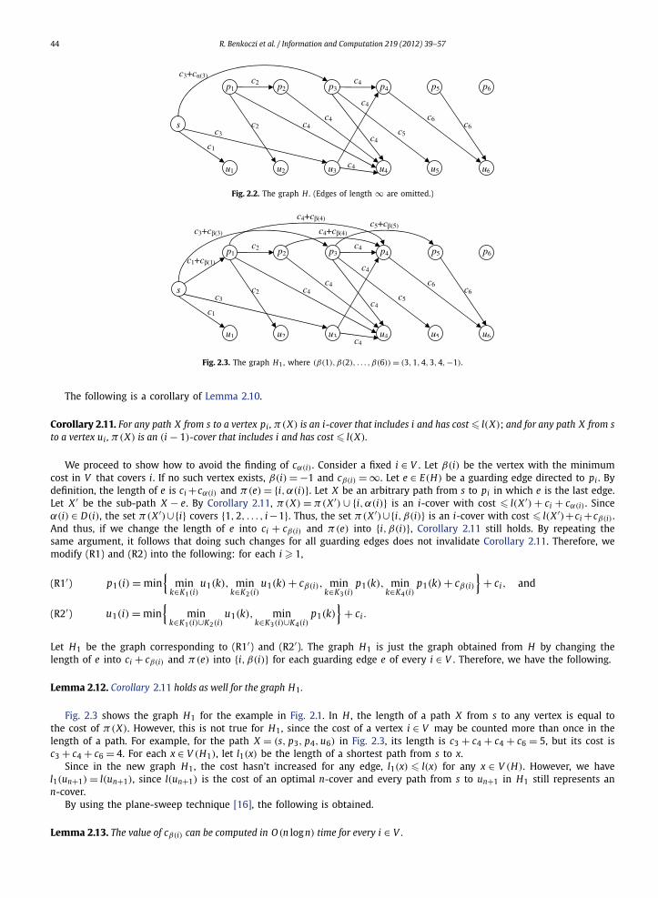
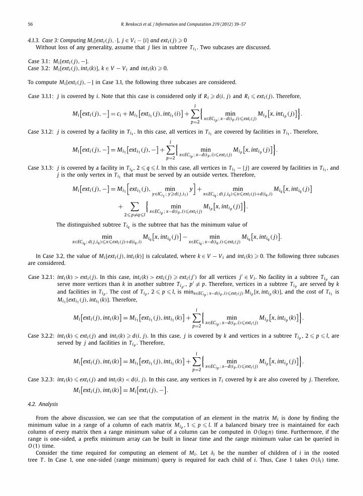
Fig. 2.3. The graph H1, where (β(1), β(2), . . . , β(6)) = (3,1,4,3,4,−1).
The following is a corollary of Lemma 2.10.
Corollary 2.11. For any path X from s to a vertex pi , π(X) is an i-cover that includes i and has cost � l(X); and for any path X from sto a vertex ui , π(X) is an (i − 1)-cover that includes i and has cost � l(X).
We proceed to show how to avoid the finding of cα(i) . Consider a fixed i ∈ V . Let β(i) be the vertex with the minimumcost in V that covers i. If no such vertex exists, β(i) = −1 and cβ(i) = ∞. Let e ∈ E(H) be a guarding edge directed to pi . Bydefinition, the length of e is ci +cα(i) and π(e) = {i,α(i)}. Let X be an arbitrary path from s to pi in which e is the last edge.Let X ′ be the sub-path X − e. By Corollary 2.11, π(X) = π(X ′) ∪ {i,α(i)} is an i-cover with cost � l(X ′) + ci + cα(i) . Sinceα(i) ∈ D(i), the set π(X ′)∪{i} covers {1,2, . . . , i −1}. Thus, the set π(X ′)∪{i, β(i)} is an i-cover with cost � l(X ′)+ci +cβ(i) .And thus, if we change the length of e into ci + cβ(i) and π(e) into {i, β(i)}, Corollary 2.11 still holds. By repeating thesame argument, it follows that doing such changes for all guarding edges does not invalidate Corollary 2.11. Therefore, wemodify (R1) and (R2) into the following: for each i � 1,
(R1′) p1(i) = min{
mink∈K1(i)
u1(k), mink∈K2(i)
u1(k) + cβ(i), mink∈K3(i)
p1(k), mink∈K4(i)
p1(k) + cβ(i)
}+ ci, and
(R2′) u1(i) = min{
mink∈K1(i)∪K2(i)
u1(k), mink∈K3(i)∪K4(i)
p1(k)}
+ ci .
Let H1 be the graph corresponding to (R1′) and (R2′). The graph H1 is just the graph obtained from H by changing thelength of e into ci + cβ(i) and π(e) into {i, β(i)} for each guarding edge e of every i ∈ V . Therefore, we have the following.
Lemma 2.12. Corollary 2.11 holds as well for the graph H1 .
Fig. 2.3 shows the graph H1 for the example in Fig. 2.1. In H , the length of a path X from s to any vertex is equal tothe cost of π(X). However, this is not true for H1, since the cost of a vertex i ∈ V may be counted more than once in thelength of a path. For example, for the path X = (s, p3, p4, u6) in Fig. 2.3, its length is c3 + c4 + c4 + c6 = 5, but its cost isc3 + c4 + c6 = 4. For each x ∈ V (H1), let l1(x) be the length of a shortest path from s to x.
Since in the new graph H1, the cost hasn’t increased for any edge, l1(x) � l(x) for any x ∈ V (H). However, we havel1(un+1) = l(un+1), since l(un+1) is the cost of an optimal n-cover and every path from s to un+1 in H1 still represents ann-cover.
By using the plane-sweep technique [16], the following is obtained.
Lemma 2.13. The value of cβ(i) can be computed in O (n log n) time for every i ∈ V .
R. Benkoczi et al. / Information and Computation 219 (2012) 39–57 45
Fig. 2.4. K ′1(i), K ′
2(i), K ′3(i), K ′
4(i).
Proof. By using a heap, Q , as a priority queue, all cβ(i) can be computed as follows. Initially, Q is empty. First, by sorting,we construct a non-decreasing sequence (w1, w2, . . . , w3n) that contains all h(i), i, and g(i), i = 1,2, . . . ,n. In the sequence,for each i ∈ V , all h(k) � i appear before i and all g(k)� i appear after i. Next, from left to right, we check each w j and dothe following: if w j is some lower reach h(i), insert ci into Q ; if w j is some upper reach g(i), delete ci from Q ; and if w jis some vertex i, we first delete ci from Q , then compute cβ(i) as the minimum cost in Q , and then insert ci back to Q .The time complexity is O (n log n). Thus, the lemma holds. �Remark 2.14. With some efforts, the value of cα(i) can also be computed in O (n log n) time for every i ∈ V . However, thecomputation is more complicated. In addition, our extended star algorithm in Section 3 uses the algorithm in this sectionas a procedure. The replacement of α(i) also makes the correctness proof of our extended star algorithm easier.
2.2.2. Modifications to the recurrencesIn this section, we give two modifications to recurrences (R1′) and (R2′). The first modification reduces the computation
of each p1(i) and u1(i) into two-dimensional range minimum queries. Then, the second modification further simplifiesthe queries, so that each p1(i) and u1(i) can be computed efficiently by maintaining dynamic data structures for one-dimensional range minimum queries.
We proceed to describe the first modification. By Lemma 2.2, for any k ∈ V , if r(k) < r(i) and k /∈ D(i), we have k < i.By relaxing the constraint that r(k) < r(i) and k /∈ D(i) by the constraint that k < i, we obtain from K1(i), K2(i), K3(i), andK4(i), respectively, the following subsets: K ′
1(i) = {k | k ∈ V , k < i, g(k) � i, k � h(i)}, K ′2(i) = {k | k ∈ V , k < i, g(k) < i,
k � h(i)}, K ′3(i) = {k | k ∈ V , k < i, g(k) � i, k < h(i)}, and K ′
4(i) = {k | k ∈ V , k < i, g(k) < i, k < h(i), g(k) + 1 � h(i)}.Then, by replacing K1, K2, K3, K4 with K ′
1, K ′2, K ′
3, K ′4, respectively, in (R1′) and (R2′), we obtain the following: for each
i � 1,
(R1′′) p2(i) = min{
mink∈K ′
1(i)u2(k), min
k∈K ′2(i)
u2(k) + cβ(i), mink∈K ′
3(i)p2(k), min
k∈K ′4(i)
p2(k) + cβ(i)
}+ ci, and
(R2′′) u2(i) = min{
mink∈K ′
1(i)∪K ′2(i)
u2(k), mink∈K ′
3(i)∪K ′4(i)
p2(k)}
+ ci .
The constraints on which a vertex k ∈ V is belonging to K ′1(i), K ′
2(i), K ′3(i), and K ′
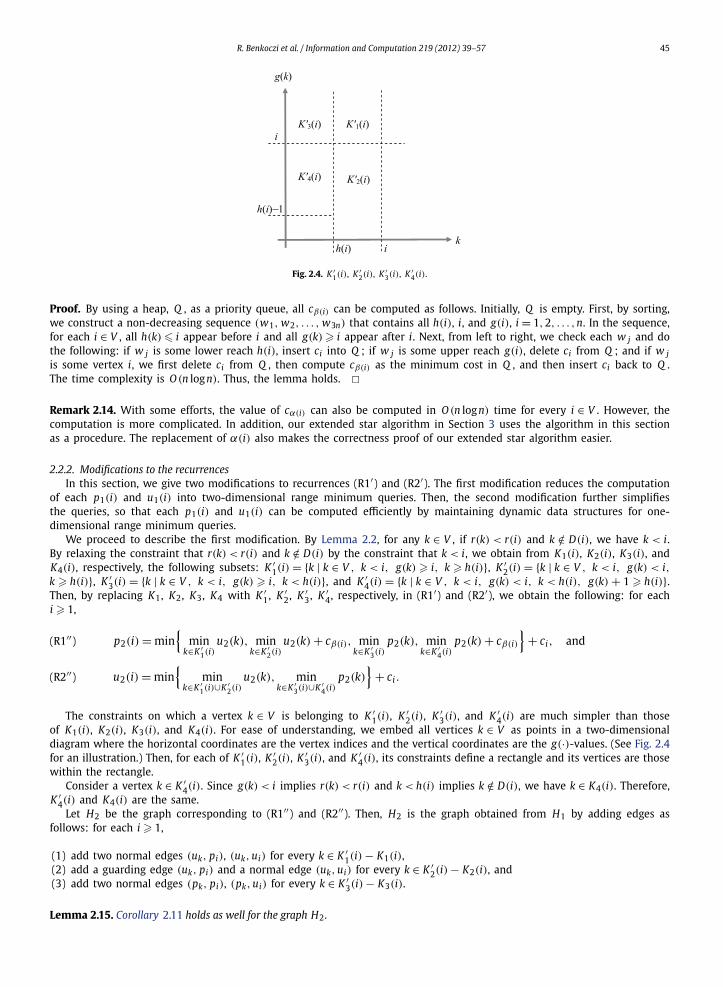
4(i) are much simpler than thoseof K1(i), K2(i), K3(i), and K4(i). For ease of understanding, we embed all vertices k ∈ V as points in a two-dimensionaldiagram where the horizontal coordinates are the vertex indices and the vertical coordinates are the g(·)-values. (See Fig. 2.4for an illustration.) Then, for each of K ′
1(i), K ′2(i), K ′
3(i), and K ′4(i), its constraints define a rectangle and its vertices are those
within the rectangle.Consider a vertex k ∈ K ′
4(i). Since g(k) < i implies r(k) < r(i) and k < h(i) implies k /∈ D(i), we have k ∈ K4(i). Therefore,K ′
4(i) and K4(i) are the same.Let H2 be the graph corresponding to (R1′′) and (R2′′). Then, H2 is the graph obtained from H1 by adding edges as
follows: for each i � 1,
(1) add two normal edges (uk, pi), (uk, ui) for every k ∈ K ′1(i) − K1(i),
(2) add a guarding edge (uk, pi) and a normal edge (uk, ui) for every k ∈ K ′2(i) − K2(i), and
(3) add two normal edges (pk, pi), (pk, ui) for every k ∈ K ′3(i) − K3(i).
Lemma 2.15. Corollary 2.11 holds as well for the graph H2 .
46 R. Benkoczi et al. / Information and Computation 219 (2012) 39–57
Fig. 2.5. K ′1(i), K ′
2(i), . . . , K ′8(i).
Proof. Consider the adding of edges in (1). Let uk be a vertex with k ∈ K ′1(i) − K1(i). Let X be any path from s to uk in H1.
By Corollary 2.11, π(X) is a (k − 1)-cover that includes k and has cost � l1(X). Since i and k cover each other, π(X) ∪ {i} isan i-cover (as well as an (i −1)-cover) that includes i and has cost � l1(X)+ci . Thus, we can add two normal edges (uk, pi),(uk, ui) in H1 without invalidating Corollary 2.11. By repeating the same argument, we conclude that after the adding of allthe edges in (1), Corollary 2.11 still holds. Similarly, the adding of edges in (2) and (3) does not invalidate Corollary 2.11.Therefore, the lemma holds. �
For each x ∈ V (H2), let l2(x) be the length of a shortest path from s to x. Since Corollary 2.11 holds for H2, l2(un+1) =l1(un+1) = l(un+1). We have the following.
Theorem 2.16. u2(n + 1) is the minimum cost of a cover of V .
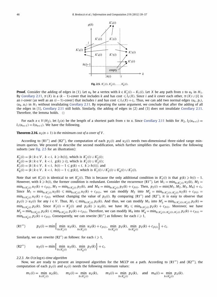
According to (R1′′) and (R2′′), the computation of each p2(i) and u2(i) needs two-dimensional three-sided range min-imum queries. We proceed to describe the second modification, which further simplifies the queries. Define the followingsubsets (see Fig. 2.5 for an illustration):
K ′5(i) = {k | k ∈ V , k < i, k � h(i)}, which is K ′
1(i) ∪ K ′2(i);
K ′6(i) = {k | k ∈ V , k < i, g(k) � i}, which is K ′
1(i) ∪ K ′3(i);
K ′7(i) = {k | k ∈ V , k < i, h(i) − 1 � g(k) < i, k � h(i)}; and
K ′8(i) = {k | k ∈ V , k < i, h(i) − 1 � g(k)}, which is K ′
1(i) ∪ K ′3(i) ∪ K ′
4(i) ∪ K ′7(i).
Note that set K ′7(i) is identical to set K ′
2(i). This is because the only additional condition in K ′7(i) is that g(k) � h(i) − 1.
However, with k � h(i), the former condition is redundant. Consider the recurrence (R1′′). Let M1 = mink∈K ′1(i) u2(k), M2 =
mink∈K ′2(i) u2(k) + cβ(i), M3 = mink∈K ′
3(i) p2(k), and M4 = mink∈K ′4(i) p2(k) + cβ(i) . Then, p2(i) = min{M1, M2, M3, M4} + ci .
Since M1 = mink∈K ′1(i) u2(k) � mink∈K ′
1(i) u2(k) + cβ(i) , we can modify M2 into M ′2 = mink∈K ′
1(i)∪K ′2(i) u2(k) + cβ(i) =
mink∈K ′5(i) u2(k) + cβ(i) without changing the value of p2(i). By comparing (R1′′) and (R2′′), it is easy to observe that
p2(i) � u2(i) for any i ∈ V . Thus, M1 � mink∈K ′1(i) p2(k). And thus, we can modify M3 into M ′
3 = mink∈K ′1(i)∪K ′
3(i) p2(k) =mink∈K ′
6(i) p2(k). Since K ′7(i) = K ′
2(i) and p2(k) � u2(k), we have M2 � mink∈K ′7(i) p2(k) + cβ(i) . Moreover, we have
M ′3 = mink∈K ′
6(i) p2(k) � mink∈K ′6(i) p2(k) + cβ(i) . Therefore, we can modify M4 into M ′
4 = mink∈K ′4(i)∪K ′
6(i)∪K ′7(i) p2(k) + cβ(i) =
mink∈K ′8(i) p2(k) + cβ(i) . Consequently, we can rewrite (R1′′) as follows: for each i � 1,
(R1′′′) p2(i) = min{
mink∈K ′
1(i)u2(k), min
k∈K ′5(i)
u2(k) + cβ(i), mink∈K ′
6(i)p2(k), min
k∈K ′8(i)
p2(k) + cβ(i)
}+ ci .
Similarly, we can rewrite (R2′′) as follows: for each i � 1,
(R2′′′) u2(i) = min{
mink∈K ′
5(i)u2(k), min
k∈K ′8(i)
p2(k)}
+ ci .
2.2.3. An O (n log n)-time algorithmNow, we are ready to present an improved algorithm for the MCCP on a path. According to (R1′′′) and (R2′′′), the
computation of each p2(i) and u2(i) needs the following minimum values:
m1(i) = mink∈K ′ (i)
u2(k), m2(i) = mink∈K ′ (i)
u2(k), m3(i) = mink∈K ′ (i)
p2(k), and m4(i) = mink∈K ′ (i)
p2(k).
1 5 6 8
R. Benkoczi et al. / Information and Computation 219 (2012) 39–57 47
To obtain these minimum values, three segment trees [16] T1, T2, T3, are maintained. The segment trees are used asdynamic data structures for (one-dimensional) range minimum queries. For ease of presentation, define the following threeoperations:
BuildTree(S): build a segment tree T on a given set S = {(k, xk, yk) | k ∈ V }, where xk and yk are, respectively, the key andvalue of vertex k;
RangeMin(T ,a,b): return the smallest value in {yk | a � xk � b, k ∈ V }; andUpdate(T ,k, y): change the value of yk into y.
Each of T1, T2, and T3 maintains a dynamic subset of vertices. The trees T1 and T2 are used, respectively, for the compu-tation of m1(i) and m2(i). Each vertex k in T1 and T2 has value u2(k). The tree T3 is used for the computation of m3(i)and m4(i). Each vertex k in T3 has value p2(k). In our implementation, the insertion of a vertex k is done by updatingits value into u2(k) or p2(k), and the deletion is done by updating its value into ∞. Initially, we create three empty treesT1 = BuildTree({(k,k,∞) | k ∈ V }), T2 = BuildTree({(k,k,∞) | k ∈ V }), and T3 = BuildTree({(k, g(k),∞) | k ∈ V }). Note that inT1 and T2, vertices are maintained in increasing order of k; while in T3, vertices are maintained in increasing order of g(k).In addition, we insert vertex 0 into T2 and T3 by Update(T2,0, u2(0)) and Update(T3,0, p2(0)). After the initialization, thesets of vertices stored in T1, T2, and T3 are, respectively, ∅, {0}, and {0}. Iteratively, our algorithm computes p2(i) and u2(i)for i = 1,2, . . . ,n + 1. In the course of the algorithm, the following invariant is maintained.
Invariant (I). At the beginning of the ith iteration, the sets of vertices stored in T1, T2, and T3 are, respectively, {k | k ∈ V ,
k < i, g(k) � i}, {k | k ∈ V , k < i}, and {k | k ∈ V , k < i}.
Note that according to the invariant (I), at the beginning of the ith iteration, the sets of three-tuples maintained in T1,T2, and T3 are, respectively, {(k,k, u2(k)) | k ∈ V , k < i, g(k) � i}, {(k,k, u2(k)) | k ∈ V , k < i}, and {(k, g(k), p2(k)) | k ∈ V ,
k < i}.With the invariant (I), it is easy to check that m1(i) = RangeMin(T1,h(i),n), m2(i) = RangeMin(T2,h(i),n), m3(i) =
RangeMin(T3, i,n), and m4(i) = RangeMin(T3,h(i) − 1,n). For i = 1, {k | k ∈ V , k < i, g(k) � i} = ∅, {k | k ∈ V , k < i} = {0},and {k | k ∈ V , k < i} = {0}. Thus, after the initialization of T1, T2, and T3, the invariant (I) is true for i = 1. At the ithiteration, 1 � i � n, we maintain the invariant for the next iteration as follows. First, we insert i into T1, T2, and T3 byUpdate(T1, i, u2(i)), Update(T2, i, u2(i)), and Update(T3, i, p2(i)). Clearly, after the insertions, the invariant of T2 and T3holds for i + 1. To maintain the invariant of T1 for i + 1, we need to further remove all vertices k with g(k) = i in it.Therefore, for each such k, we perform Update(T1,k,∞) to remove it.
Our algorithm is formally presented as follows.
Algorithm 2.1 (CONDITIONAL_COVERING_PATH).Input: a path graph with vertex set V = {1,2, . . . ,n} and edge set E = {(1,2), (2,3), . . . , (n − 1,n)}Output: the minimum cost of a cover of Vbegin
1 (c0, R0,d(0,1), g(0), p2(0), u2(0)) ← (0,0,∞, 0,0,0); (cn+1, Rn+1,d(n, (n + 1))) ← (0,0,∞)
2 compute h(i), g(i), and cβ(i) for each i, 1 � i � n3 T1 ← BuildTree({(k,k,∞) | 0 � k � n})4 T2 ← BuildTree({(k,k,∞) | 0 � k � n}); Update(T2,0, u2(0))
5 T3 ← BuildTree({(k, g(k),∞) | 0 � k � n}); Update(T3,0, p2(0))
6 for i ← 1 to n do7 begin8 m1 ← RangeMin(T1,h(i),n) //* m1 = mink∈K ′
1(i) u2(k)
9 m2 ← RangeMin(T2,h(i),n) //* m2 = mink∈K ′5(i) u2(k)
10 m3 ← RangeMin(T3, i,n) //* m3 = mink∈K ′6(i) p2(k)
11 m4 ← RangeMin(T3,h(i) − 1,n) //* m4 = mink∈K ′8(i) p2(k)
12 p2(i) ← min{m1,m2 + cβ(i),m3,m4 + cβ(i)} + ci13 u2(i) ← min{m2,m4} + ci14 Update(T1, i, u2(i)); Update(T2, i, u2(i)); Update(T3, i, p2(i)) //* insert i15 for each k with g(k) = i do Update(T1,k,∞) //* delete all k with g(k) = i16 end17 u2(n + 1) ← RangeMin(T3,n,n) //* since K ′
5(n + 1) = ∅ and cn+1 = 018 return (u2(n + 1))
end
The correctness of Algorithm 2.1 is ensured by Theorem 2.16, (R1′′′), (R2′′′), and the invariant (I). The time complexityis analyzed as follows. Line 1 takes O (1) time. By sorting, all h(i) and g(i) can be determined in O (n log n) time. ByLemma 2.13, all cβ(i) can be computed in O (n log n) time. Thus, Line 2 takes O (n log n) time. Each BuildTree operation needs
48 R. Benkoczi et al. / Information and Computation 219 (2012) 39–57
O (n log n) time, and each Update and RangeMin operation needs O (log n) time [16]. Thus, Lines 3–5 require O (n log n)
time. Consider the for-loop in Lines 6–16. At the ith iteration, we need to perform four RangeMin operations and qi + 3Update operations, where qi is the number of Update operations performed in Line 15. Each Update operation in Line 15corresponds to the deletion of a vertex k from T1. Each vertex k may be deleted from T1 at most once. Thus, (q1 + q2 +· · · + qn+1) � n. And therefore, the for-loop requires O (n log n) time in total. Line 17 takes O (log n) time. Consequently, thetime complexity of Algorithm 2.1 is O (n log n). Therefore, we have the following.
Theorem 2.17. The MCCP on a path can be solved in O (n log n) time.
2.3. An extension to cycles
A simple extension of our algorithm for a path network to a cycle (i.e., vertex 1 and n are linked by an edge) is brieflydescribed as follows.
Here a facility i of a solution is critical if there is no other facility k in the solution such that the set of vertices withinthe coverage of i is a proper subset of the set of vertices within the coverage of k. The algorithm is to consider each vertexas a critical facility in an optimal solution. When a vertex i is considered, we remove i from the cycle. Let L be the totallength of the cycle. We assume that Ri is not larger than L/2. In case this is not true, since all vertices are within thecoverage of i, we simply set Ri to be L/2. Let j and j′ be the two vertices adjacent to i in the cycle. Two similar casesabout k, that is opened to cover i, are considered: (i) the shortest path from k to i goes through j, and (ii) the shortestpath from k to i goes through j′ . It is sufficient to only consider (i). For (i), we let j′ designate the beginning of the pathobtained with removal of i and j designate the end of the path. Two imaginary vertices, say i′ and i′′ , are inserted at thebeginning of the path and one imaginary vertex, say i′′′ , is attached at the end of the path, where ci′ = ci′′ = ci′′′ = 0, Ri′ = 0,Ri′′ = Ri′′′ = Ri , d(i′, i′′) = 0, d(i′′, j′) = d(i, j′), and d( j, i′′′) = d( j, i). Note that since Ri � L/2, i′′ cannot cover i′′′ and thusi′′′ needs to be covered by another facility k. Obviously, the optimal cost for the cycle when i is opened as a critical facilityis equal to p2(i′′′) + ci . In this way, the MCCP on a cycle can be solved in O (n2 logn) time.
Theorem 2.18. The MCCP on a cycle can be solved in O (n2 logn) time.
3. Extended star networks
An extended star is a network in which three or more paths are connected by a single root vertex, which we la-bel n. Horne and Smith [6] had an O (n2)-time algorithm for the MCCP on an extended star G = (V , E). In this section,an O (n1.5 logn)-time algorithm is presented.
Let χ1,χ2, . . . ,χτ be the branches of the root vertex n, where τ is the number of branches in G . Each branch χ jcontains the set V j of vertices on the path from a leaf vertex j(1) to vertex j(n j), where n j is the number of vertices on thebranch χ j . Note that each j(n j) is adjacent to n. For each vertex i ∈ V , define the external coverage of i as ext(i) = Ri −d(i,n).This measure represents the amount of coverage which vertex i can provide into branches not containing i.
The following property is easy to obtain.
Observation 3.1. In any optimal solution, there exists a vertex i ∈ V such that ext(i) � 0 and no facility is located at a vertexi′ ∈ V with ext(i′) > ext(i).
Any vertex that satisfies these conditions is called an external covering vertex.
Case 1: n is an external covering vertex. In this case, if a vertex in V j is not covered by n, then it has to be covered byfacilities in V j , 1 � j � τ .
Case 2: ω �= n is an external covering vertex. Note that ext(ω) � 0. Assume that ω is on a branch χt , 1 � t � τ . In this case,vertices in Vt (possibly except ω) are covered by facilities in Vt ; and if a vertex in V j , 1 � j �= t � τ , is not coveredby ω, it has to be covered by facilities in V j .
Let p∗(ω) denote the optimal cost when ω is an external covering vertex. Then the optimal cost is minω∈V p∗(ω).
Pseudo vertices. We observe that if a vertex in a branch is not covered by facilities located in the branch, it has to becovered by the external covering vertex ω. Hence a pseudo vertex j(n+
j ) is introduced for each branch χ j to simulate the
external covering vertex ω located outside χ j . The pseudo vertex j(n+j ) is appended after vertex j(n j).
For each j, j = 1,2, . . . , τ , the open-facility cost c j(n+j ) of j(n+
j ) is set to zero. The coverage radius of j(n+j ) and the
distance d( j(n j), j(n+j )) are not fixed. They are respectively assigned to be Rω and d( j(n j),ω) in the original star graph,
when an external covering vertex ω is given. We consider each branch as a path. Let u j,2(ω) denote the value of u2(n+) and
j
R. Benkoczi et al. / Information and Computation 219 (2012) 39–57 49
p j,2(ω) denote the value of p2(n+j ) for a given external covering vertex ω. Then, u j,2(ω) + cω is the optimal cost to cover
all vertices in V j with facility ω and facilities in V j and p j,2(ω) + cω is the optimal cost to cover all vertices in V j ∪ {ω}with facility ω and facilities in V j .
In Section 3.1, for each branch χ j , 1 � j � τ , we first show how to modify Algorithm 2.1 such that the values of u j,2(ω)
and p j,2(ω) can be computed in O (n log n) time for all vertices ω ∈ V \V j . Then, in Sections 3.2 and 3.3, we present twomethods to efficiently compute the costs p∗(ω), ω ∈ V .
3.1. Computing u2(n+j ) and p2(n
+j ), 1 � j � τ
For all i, 1 � i � n j , we can compute the p2(·) and u2(·) values of vertices j(1), j(2), . . . , j(n j) in O (n j logn j) time byAlgorithm 2.1. However, two problems appear after j(n+
j ) is introduced in the path. Both of them stem from the following
fact: Computing u2(n+j ) and p2(n
+j ) for all possible values of ω, if naively done, will take O (n2 log n) time. To overcome
these problems, the majority of computation involved in finding u2(n+j ) and p2(n
+j ) must be performed without knowing
what ω is, i.e., the radius and distance details of j(n+j ).
The first problem is that, in Algorithm 2.1, we need to compute β-values of vertices for the computation of correspondingprotected costs. Without knowing the coverage of j(n+
j ), the β-values of vertices that can be covered by j(n+j ) cannot be
determined correctly. More specifically, since c j(n+j ) = 0, the β-values of these vertices should be zero. Actually, this problem
can be ignored since we only need the correct computation of u2(n+j ) and p2(n
+j ). In the following, we show that the
protected and unprotected costs needed for the computation of u2(n+j ) and p2(n
+j ) are all correctly computed.
Let p2(i) and u2(i) be the protected and unprotected costs of vertex j(i) on χ j , computed by Algorithm 2.1. Note that thiscomputation does not require knowledge of j(n+
j ). We denote by χ ′j the new path composed of χ j and some vertex j(n+
j );and let p′
2(i) and u′2(i) be the protected and unprotected costs of j(i) on χ ′
j . Let j(q + 1), j(q + 2), . . . , j(n j) be the vertices
covered by j(n+j ). With or without vertex j(n+
j ), the protected and unprotected costs of j(q + 1), j(q + 2), . . . , j(n j) might
be changed. However, since the protected and unprotected costs of j(1), j(2), . . . , j(q) on χ ′j are independent of j(n+
j ), wehave u′
2(i) = u2(i) and p′2(i) = p2(i) for 1 � i � q.
u2(n+j ): Let u∗ be the minimum unprotected cost of vertices j(q+1), j(q+2), . . . , j(n j) on χ ′
j . To compute u2(n+j ) correctly,
we only need to guarantee the correct computation of u∗ . Clearly, this computation does not depend on anyprotected or unprotected cost of a vertex j(i) with q + 1 � i � n j ; otherwise u∗ is not the minimum. Therefore, wecan correctly compute u2(n
+j ) using values of p2(1), p2(2), . . . , p2(n j) and u2(1), u2(2), . . . , u2(n j).
p2(n+j ): The compute p2(n
+j ), we find a vertex i in j(1), j(2), . . . , j(n j) to cover j(n+
j ) and use its protected cost if i � q orits unprotected cost if i � q + 1. Since p′
2(i) = p2(i) for 1 � i � q, we only need to consider the case i � q + 1. Inthis case, among vertices j(q + 1), j(q + 2), . . . , j(n j), we are looking for the best vertex, say k, to cover j(n+
j ) and
compute p2(n+j ) = u′
2(k). If u′2(k) depends on the protected or unprotected cost of a vertex j(k′) with 1 � k′ � q,
we have u′2(k) = u2(k) and thus p2(n
+j ) can be correctly computed. Assume that j(k) depends on the protected or
unprotected cost of a vertex j(k′) with q + 1 � k′ < k. In the following, we show that u′2(k) � u2(n
+j ) + cβ( j(n+
j )) .
First, consider the case that j(k) covers j(k′). In this case, u′2(k) = u′
2(k′)+ c j(k) . By definition, c j(k) � cβ( j(n+
j )) . Since
u′2(k
′) � u∗ � u2(n+j ), we obtain u′
2(k) � u′2(n
+j ) + cβ( j(n+
j )) . Note that p2(n+j ) � u2(n
+j ) + cβ( j(n+
j )) , since u′2(n
+j ) +
cβ( j(n+j )) corresponds to a feasible solution to p2(n
+j ). Thus, from u′
2(k) � u2(n+j ) + cβ( j(n+
j )) , we conclude that
p2(n+j ) = u2(n
+j ) + cβ( j(n+
j )) . The case that j(k) does not cover j(k′) is similar. Therefore, the correct computation
of u′2(k) is unnecessary.
The second problem that arises out of not knowing details about j(n+j ) is that we cannot directly use Algorithm 2.1 to
compute u2(n+j ) and p2(n
+j ), since the upper reach values of vertices j(1), j(2), . . . , j(n j) on χ j might be incorrect without
knowing the position of j(n+j ). In the following, we show a simple way to fix it.
For a vertex j(i), 1 � i � n+j = n j + 1, we define its lower cover h′
j(i) and upper cover g′j(i) as follows:
h′j(i) = d
(j(1), j(i)
) − R j(i); and
g′j(i) = d
(j(1), j(i)
) + R j(i).
(If we consider the vertices on χ j as a sequence of points on the real line, where each j(i) is located at position d( j(1), j(i)),then h′
j(i) and g′j(i) represent, respectively, the leftmost and rightmost points covered by j(i).) Note that the values of h′
j(·)and g′ (·) of a vertex are not affected by the position of j(n+). Accordingly, we redefine the subsets K ′ (·), K ′ (·), K ′ (·),
j j 1 5 6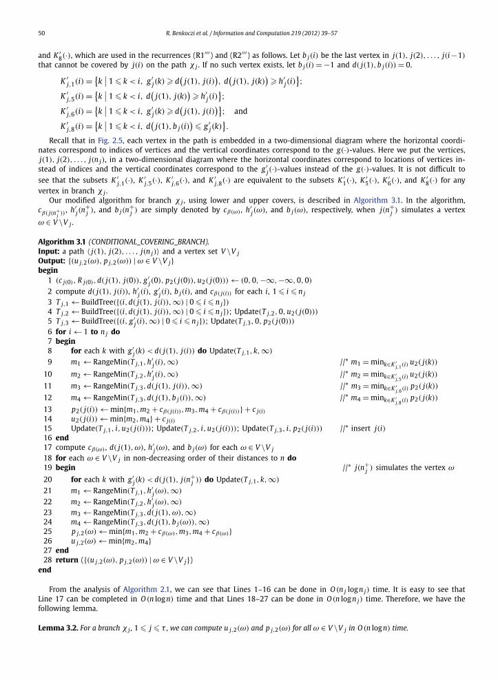
50 R. Benkoczi et al. / Information and Computation 219 (2012) 39–57
and K ′8(·), which are used in the recurrences (R1′′′) and (R2′′′) as follows. Let b j(i) be the last vertex in j(1), j(2), . . . , j(i−1)
that cannot be covered by j(i) on the path χ j . If no such vertex exists, let b j(i) = −1 and d( j(1),b j(i)) = 0.
K ′j,1(i) = {
k∣∣ 1 � k < i, g′
j(k) � d(
j(1), j(i)), d
(j(1), j(k)
)� h′
j(i)};
K ′j,5(i) = {
k∣∣ 1 � k < i, d
(j(1), j(k)
)� h′
j(i)};
K ′j,6(i) = {
k∣∣ 1 � k < i, g′
j(k) � d(
j(1), j(i))}; and
K ′j,8(i) = {
k∣∣ 1 � k < i, d
(j(1),b j(i)
)� g′
j(k)}.
Recall that in Fig. 2.5, each vertex in the path is embedded in a two-dimensional diagram where the horizontal coordi-nates correspond to indices of vertices and the vertical coordinates correspond to the g(·)-values. Here we put the vertices,j(1), j(2), . . . , j(n j), in a two-dimensional diagram where the horizontal coordinates correspond to locations of vertices in-stead of indices and the vertical coordinates correspond to the g′
j(·)-values instead of the g(·)-values. It is not difficult tosee that the subsets K ′
j,1(·), K ′j,5(·), K ′
j,6(·), and K ′j,8(·) are equivalent to the subsets K ′
1(·), K ′5(·), K ′
6(·), and K ′8(·) for any
vertex in branch χ j .Our modified algorithm for branch χ j , using lower and upper covers, is described in Algorithm 3.1. In the algorithm,
cβ( j(n+j )) , h′
j(n+j ), and b j(n
+j ) are simply denoted by cβ(ω) , h′
j(ω), and b j(ω), respectively, when j(n+j ) simulates a vertex
ω ∈ V \V j .
Algorithm 3.1 (CONDITIONAL_COVERING_BRANCH).Input: a path 〈 j(1), j(2), . . . , j(n j)〉 and a vertex set V \V jOutput: {(u j,2(ω), p j,2(ω)) | ω ∈ V \V j}begin
1 (c j(0), R j(0),d( j(1), j(0)), g′j(0), p2( j(0)), u2( j(0))) ← (0,0,−∞,−∞,0,0)
2 compute d( j(1), j(i)), h′j(i), g′
j(i), b j(i), and cβ( j(i)) for each i, 1 � i � n j
3 T j,1 ← BuildTree({(i,d( j(1), j(i)),∞) | 0 � i � n j})4 T j,2 ← BuildTree({(i,d( j(1), j(i)),∞) | 0 � i � n j}); Update(T j,2,0, u2( j(0)))
5 T j,3 ← BuildTree({(i, g′j(i),∞) | 0 � i � n j}); Update(T j,3,0, p2( j(0)))
6 for i ← 1 to n j do7 begin8 for each k with g′
j(k) < d( j(1), j(i)) do Update(T j,1,k,∞)
9 m1 ← RangeMin(T j,1,h′j(i),∞) //* m1 = mink∈K ′
j,1(i) u2( j(k))
10 m2 ← RangeMin(T j,2,h′j(i),∞) //* m2 = mink∈K ′
j,5(i) u2( j(k))
11 m3 ← RangeMin(T j,3,d( j(1), j(i)),∞) //* m3 = mink∈K ′j,6(i) p2( j(k))
12 m4 ← RangeMin(T j,3,d( j(1),b j(i)),∞) //* m4 = mink∈K ′j,8(i) p2( j(k))
13 p2( j(i)) ← min{m1,m2 + cβ( j(i)),m3,m4 + cβ( j(i))} + c j(i)14 u2( j(i)) ← min{m2,m4} + c j(i)15 Update(T j,1, i, u2( j(i))); Update(T j,2, i, u2( j(i))); Update(T j,3, i, p2( j(i))) //* insert j(i)16 end17 compute cβ(ω) , d( j(1),ω), h′
j(ω), and b j(ω) for each ω ∈ V \V j
18 for each ω ∈ V \V j in non-decreasing order of their distances to n do19 begin //* j(n+
j ) simulates the vertex ω
20 for each k with g′j(k) < d( j(1), j(n+
j )) do Update(T j,1,k,∞)
21 m1 ← RangeMin(T j,1,h′j(ω),∞)
22 m2 ← RangeMin(T j,2,h′j(ω),∞)
23 m3 ← RangeMin(T j,3,d( j(1),ω),∞)
24 m4 ← RangeMin(T j,3,d( j(1),b j(ω)),∞)
25 p j,2(ω) ← min{m1,m2 + cβ(ω),m3,m4 + cβ(ω)}26 u j,2(ω) ← min{m2,m4}27 end28 return ({(u j,2(ω), p j,2(ω)) | ω ∈ V \V j})
end
From the analysis of Algorithm 2.1, we can see that Lines 1–16 can be done in O (n j logn j) time. It is easy to see thatLine 17 can be completed in O (n log n) time and that Lines 18–27 can be done in O (n log n j) time. Therefore, we have thefollowing lemma.
Lemma 3.2. For a branch χ j , 1 � j � τ , we can compute u j,2(ω) and p j,2(ω) for all ω ∈ V \V j in O (n log n) time.
R. Benkoczi et al. / Information and Computation 219 (2012) 39–57 51
3.2. An O (nτ log n) algorithm
To meet the constraint of the MCCP, an external covering vertex itself must be covered by some other facility. Recall thatwe have two cases regarding the external covering vertex.
Case 1: n is an external covering vertex. In this case, one branch, say χk , is needed to contribute a facility to cover n.The cost of branch χk is then equal to pk,2(n). The cost of any other branch χ j , 1 � j �= k � τ , is equal to u j,2(n). Thus, thetotal cost is
cn + pk,2(n) − uk,2(n) +∑
1� j�τ
u j,2(n).
Clearly, the distinguished branch χk is the branch that has the minimum value of pk,2(n) − uk,2(n).
Case 2: ω �= n is an external covering vertex. Assume that the external covering vertex ω is located in a branch χt ,1 � t � τ . Note that ext(ω) � 0. We consider the following three subcases.
Case 2.1: ω is covered by n;Case 2.2: ω is covered by some facility in χt ; andCase 2.3: ω is covered by some facility in χk , 1 � k �= t � τ .
In Case 2.1, the cost of χt is u2(ω), the cost of χ j , 1 � j �= t � τ , is u j,2(ω), and the total cost is cn + u2(ω) +∑1� j �=t�τ u j,2(ω). In Case 2.2, the cost of χt is p2(ω), the cost of χ j , 1 � j �= t � τ , is u j,2(ω), and the total cost is
p2(ω) + ∑1� j �=t�τ u j,2(ω). In Case 2.3, the cost of χt is u2(ω), the cost of χk is pk,2(ω), and for each branch χ j , 1 � j � τ
and j �= t,k, its cost is u j,2(ω). Thus, the total cost in Case 2.3 is
u2(ω) + pk,2(ω) − uk,2(ω) +∑
1� j �=t�τ
u j,2(ω).
Therefore, the distinguished branch χk is the branch (except χt ) that has the minimum value of pk,2(ω) − uk,2(ω).Our first algorithm for computing the cost of p∗(ω) is presented as follows. For brevity, only the computation of p∗(ω)
for Case 2.3 is described. For each vertex ω ∈ V , we maintain three variables: x(ω), y(ω), and z(ω), which are used torecord, respectively, the values of u2(ω), min1�k �=t�τ {pk,2(ω)− uk,2(ω)}, and
∑1� j �=t�τ u j,2(ω), where t is the index of the
branch containing ω. Initially, set y(ω) = ∞ and z(ω) = 0. Next, we repeatedly perform Algorithm 3.1 on each branch χ j ,j = 1,2, . . . , τ , and do the following: for each v ∈ V j , store u2(v) into x(v); and for each ω ∈ V \V j , update y(ω) intomin{y(ω), p j,2(ω) − u j,2(ω)} and add u j,2(ω) into z(ω). Finally, we compute p∗(ω) = x(ω) + y(ω) + z(ω) each ω ∈ V .
By Lemma 3.2, the overall time complexity is O (nτ logn). Therefore, in O (nτ log n) time, we can compute the value ofminω∈V p∗(ω).
Theorem 3.3. The MCCP on an extended star can be solved in O (nτ logn) time, where τ is the number of branches in the extendedstar.
3.3. An O (n1.5 log n) algorithm
Our first algorithm for the MCCP on an extended star requires O (nτ logn) time. In the worst case, τ is O (n). Next, wepresent another algorithm which runs in O (n1.5 log n) time.
We separate the set of branches in G into two classes according to their sizes. If a branch contains at least n0.5 vertices,we call it a big branch, and the branch is called a small branch, otherwise. The number of big branches in G is no morethan n0.5. For all ω, the values p j,2(ω) and u j,2(ω) of all the big branches can be computed in O (n1.5 logn) time by usingthe result in Lemma 3.2.
In the following, we create a data structure to merge the information contained in all small branches, which can answera total cost (of these small branches) query in amortized O (n0.5 logn) time, for any given external covering vertex.
For brevity, we only consider Case 2, in which the external covering vertex ω is located in a branch χt , 1 � t � τ . Foreach branch χ j , 1 � j � τ , we first show that there are at most (n j + 1)2 possible different pairs of values of p j,2(ω)
and u j,2(ω) for all ω ∈ V \V j as follows. As demonstrated in Fig. 3.1(a), we draw horizontal and vertical lines throughn j points in the two-dimensional diagram for the branch χ j , in which each vertex j(i) ∈ V j is represented as the point(d( j(1), j(i)), g′
j( j(i))). This produces a mesh, denoted by M j , of at most (n j + 1)2 rectangular cells. We assume that eachcell is only associated with its upper boundary and right boundary.
It is not difficult to see that K ′j,1(n
+j ), K ′
j,5(n+j ), and K ′
j,6(n+j ) stay unchanged when (h′
j(n+j ),d( j(1),n+
j )) lies in a cell.
By definition, d( j(1),b j(n+j )) stays unchanged when (h′
j(n+j ),d( j(1),n+
j )) lies in a column. Therefore, K ′j,8(n
+j ) also stays
unchanged in a cell. It implies that there are at most (n j +1)2 possible pairs of values of p j,2(n+j ), u j,2(n
+j ). In our algorithm,
we pre-compute all these (n j + 1)2 possible pairs for all small branches χ j , 1 � j � τ .
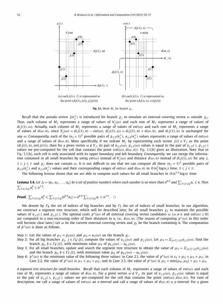
52 R. Benkoczi et al. / Information and Computation 219 (2012) 39–57
Fig. 3.1. Mesh M j for branch χ j .
Recall that the pseudo vertex j(n+j ) is introduced for branch χ j to simulate an external covering vertex ω outside χ j .
Thus, each column of M j represents a range of values of h′j(ω) and each row of M j represents a range of values of
d( j(1),ω). Actually, each column of M j represents a range of values of ext(ω) and each row of M j represents a rangeof values of d(ω,n), since h′
j(ω) = d( j(1),n) − ext(ω), d( j(1),ω) = d( j(1),n) + d(ω,n), and d( j(1),n) is unchanged for
any ω. Consequently, each of the (n j + 1)2 possible pairs of p j,2(n+j ), u j,2(n
+j ) values represents a range of values of ext(ω)
and a range of values of d(ω,n). More specifically, if we redraw M j by representing each vertex j(i) ∈ V j as the point(d( j(i),n), ext( j(i))), then for a given vertex ω /∈ V j , its pair of u j,2(ω), p j,2(ω) values is equal to the pair of u j,2(·), p j,2(·)values we pre-computed for the cell that contains the point (ext(ω),d(ω,n)). Fig. 3.1(b) gives an illustration. Note that inFig. 3.1(b), each cell is only associated with its upper boundary and left boundary. Consequently, we can merge the informa-tion contained in all small branches by using ext(ω) instead of h′
j(ω) and distance d(ω,n) instead of d( j(1),ω) for any j,
1 � j � τ and χ j does not contain ω. It is not difficult to see that we can compute all these (n j + 1)2 possible pairs ofp j,2(n
+j ) and u j,2(n
+j ) values and their corresponding ranges of ext(ω) and d(ω,n) in O (n2
j log n j) time, 1 � j � τ .
The following lemma shows that we are able to compute such values for all small branches in O (n1.5 log n) time.
Lemma 3.4. Let � = {a1,a2, . . . ,aq} be a set of positive numbers where each number is no more than n0.5 and∑
1�i�q ai � n. Then∑1�i�q a2
i � n1.5 .
Proof.∑
1�i�q a2i �
∑1�i�q{n0.5ai} = n0.5 ∑
1�i�q ai � n1.5. �We denote by ΓB the set of indices of big branches and by ΓS the set of indices of small branches. In our algorithm,
we construct a segment tree structure, which will be described later, for all small branches χ j to maintain the possiblevalues of u j,2(·) and p j,2(·). The optimal costs p∗(ω) of all external covering vertex candidates ω (ω �= n and ext(ω) � 0)are computed in a non-increasing order of their distances to n, i.e., d(ω,n). (The reason of computing p∗(ω) in this orderwill become clear later.) Let ω be the current external covering vertex and χt be the branch containing it. The computationof p∗(ω) is done as follows.
Step 1: Get the values of μ1 = p2(ω) and μ2 = u2(ω) on the branch χt .Step 2: For all big branches χ j , j ∈ ΓB\{t}, compute the values of u j,2(ω) and p j,2(ω). Let μ3 = Σ j∈Γ1\{t}u j,2(ω). Find the
branch χk , k ∈ ΓB\{t}, with minimum value μ4 of pk,2(ω) − uk,2(ω).Step 3: For all small branches, update and search the segment tree structure to obtain the value of μ5 = Σ j∈Γ2\{t}u j,2(ω)
and the branch χk , k ∈ ΓS\{t}, with minimum value μ6 of pk,2(ω) − uk,2(ω).Step 4: p∗(ω) is the minimum value of the following three values: in Case 2.1, the value of p∗(ω) is cn + μ2 + μ3 + μ5; in
Case 2.2, the value of p∗(ω) is μ1 + μ3 + μ5; and in Case 2.3, the value of p∗(ω) is μ2 + min{μ4,μ6} + μ3 + μ5.
A segment tree structure for small branches Recall that each column of M j represents a range of values of ext(ω) and eachrow of M j represents a range of values of d(ω,n). For a given vertex ω /∈ V j , its pair of u j,2(ω), p j,2(ω) values is equalto the pair of u j,2(·), p j,2(·) values we pre-computed for the cell that contains the point (ext(ω),d(ω,n)). For ease ofdescription, we call a range of values of ext(ω) an x-interval and call a range of values of d(ω,n) a y-interval. For a given
R. Benkoczi et al. / Information and Computation 219 (2012) 39–57 53
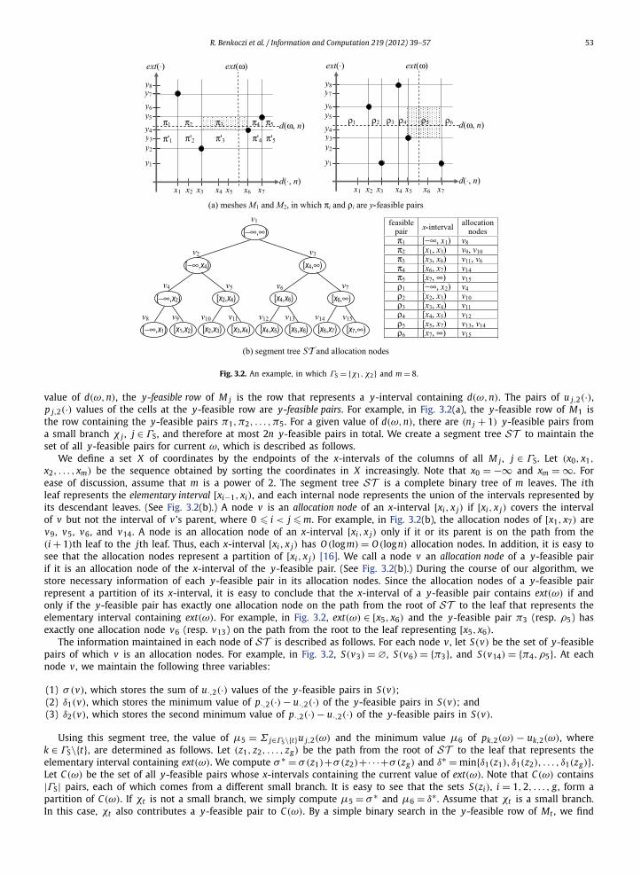
Fig. 3.2. An example, in which ΓS = {χ1,χ2} and m = 8.
value of d(ω,n), the y-feasible row of M j is the row that represents a y-interval containing d(ω,n). The pairs of u j,2(·),p j,2(·) values of the cells at the y-feasible row are y-feasible pairs. For example, in Fig. 3.2(a), the y-feasible row of M1 isthe row containing the y-feasible pairs π1,π2, . . . ,π5. For a given value of d(ω,n), there are (n j + 1) y-feasible pairs froma small branch χ j , j ∈ ΓS, and therefore at most 2n y-feasible pairs in total. We create a segment tree ST to maintain theset of all y-feasible pairs for current ω, which is described as follows.
We define a set X of coordinates by the endpoints of the x-intervals of the columns of all M j , j ∈ ΓS. Let (x0, x1,
x2, . . . , xm) be the sequence obtained by sorting the coordinates in X increasingly. Note that x0 = −∞ and xm = ∞. Forease of discussion, assume that m is a power of 2. The segment tree ST is a complete binary tree of m leaves. The ithleaf represents the elementary interval [xi−1, xi), and each internal node represents the union of the intervals represented byits descendant leaves. (See Fig. 3.2(b).) A node v is an allocation node of an x-interval [xi, x j) if [xi, x j) covers the intervalof v but not the interval of v ’s parent, where 0 � i < j � m. For example, in Fig. 3.2(b), the allocation nodes of [x1, x7) arev9, v5, v6, and v14. A node is an allocation node of an x-interval [xi, x j) only if it or its parent is on the path from the(i + 1)th leaf to the jth leaf. Thus, each x-interval [xi, x j) has O (log m) = O (log n) allocation nodes. In addition, it is easy tosee that the allocation nodes represent a partition of [xi, x j) [16]. We call a node v an allocation node of a y-feasible pairif it is an allocation node of the x-interval of the y-feasible pair. (See Fig. 3.2(b).) During the course of our algorithm, westore necessary information of each y-feasible pair in its allocation nodes. Since the allocation nodes of a y-feasible pairrepresent a partition of its x-interval, it is easy to conclude that the x-interval of a y-feasible pair contains ext(ω) if andonly if the y-feasible pair has exactly one allocation node on the path from the root of ST to the leaf that represents theelementary interval containing ext(ω). For example, in Fig. 3.2, ext(ω) ∈ [x5, x6) and the y-feasible pair π3 (resp. ρ5) hasexactly one allocation node v6 (resp. v13) on the path from the root to the leaf representing [x5, x6).
The information maintained in each node of ST is described as follows. For each node v , let S(v) be the set of y-feasiblepairs of which v is an allocation nodes. For example, in Fig. 3.2, S(v3) = ∅, S(v6) = {π3}, and S(v14) = {π4,ρ5}. At eachnode v , we maintain the following three variables:
(1) σ(v), which stores the sum of u·,2(·) values of the y-feasible pairs in S(v);(2) δ1(v), which stores the minimum value of p·,2(·) − u·,2(·) of the y-feasible pairs in S(v); and(3) δ2(v), which stores the second minimum value of p·,2(·) − u·,2(·) of the y-feasible pairs in S(v).
Using this segment tree, the value of μ5 = Σ j∈ΓS\{t}u j,2(ω) and the minimum value μ6 of pk,2(ω) − uk,2(ω), wherek ∈ ΓS\{t}, are determined as follows. Let (z1, z2, . . . , zg) be the path from the root of ST to the leaf that represents theelementary interval containing ext(ω). We compute σ ∗ = σ(z1)+σ(z2)+· · ·+σ(zg) and δ∗ = min{δ1(z1), δ1(z2), . . . , δ1(zg)}.Let C(ω) be the set of all y-feasible pairs whose x-intervals containing the current value of ext(ω). Note that C(ω) contains|ΓS| pairs, each of which comes from a different small branch. It is easy to see that the sets S(zi), i = 1,2, . . . , g , form apartition of C(ω). If χt is not a small branch, we simply compute μ5 = σ ∗ and μ6 = δ∗ . Assume that χt is a small branch.In this case, χt also contributes a y-feasible pair to C(ω). By a simple binary search in the y-feasible row of Mt , we find
54 R. Benkoczi et al. / Information and Computation 219 (2012) 39–57
the cell containing (ext(ω),d(ω,n)), and denote its ut,2(·) and pt,2(·) values by u′ and p′ , respectively. Then, we computeμ5 = σ ∗ − u′ and determine the value of μ6 as follows: if u′ − p′ �= δ∗ , μ6 = δ∗; otherwise, μ6 is the second minimum in{δ1(z1), δ2(z1), δ1(z2), δ2(z2), . . . , δ1(zg), δ2(zg)}. Clearly, the above computation of μ5 and μ6 takes O (log n) time.
Next, we show how to maintain the values of σ(v), δ1(v), and δ2(v) at each node v . Initially, we store all y-feasible pairscorresponding to d(ω,n) = ∞ into ST . Since each of the y-feasible pairs has O (log n) allocation nodes, this initializationrequires O (n log n) time. When the value of d(ω,n) decreases, the y-feasible row of some small branch χ j may change, inwhich case, we need to delete the n j + 1 pairs of the old y-feasible row and insert the n j + 1 pairs of the new y-feasiblerow into the segment tree. For example, in Fig. 3.2(a), when the value of d(ω,n) decreases to a value in (y2, y4], weneed to delete the pairs π1,π2, . . . ,π5 and insert the pairs π ′
1,π′2, . . . ,π
′5 into the segment tree. We have the following
observations.
(1) The u j,2(·) values of the cells at the same column of M j are all the same. The reason is that the only factor affectingunprotected cost is the external coverage, not the location of external vertex; and
(2) The p j,2(·) values of the cells at the same column of M j are non-increasing from top to bottom. The reason is that thecost for χ j to provide a facility to cover an external vertex ω increases when the distance d(ω,n) increases. Therefore,the p j,2(·) − u j,2(·) values of the same column of M j are non-increasing from top to down.
Assume that the y-feasible row of M j changes. Consider the deletion of a pair (u, p) of the old y-feasible row. There isa pair (u′, p′) of the new y-feasible row such that (u, p) and (u′, p′) are belonging to two cells at the same column. Forexample, in Fig. 3.2(a), if (u, p) = π2, then (u′, p′) is the pair π ′
2. Let v be an allocation node of (u, p). Obviously, v is alsoan allocation node of (u′, p′). For the deletion of (u, p), we need to subtract u from σ(v); for the insertion of (u′, p′), weneed to add u′ to σ(v). However, according to (1), we have u′ = u. Thus, the value of σ(v) is unchanged after the deletionof (u, p) and the insertion of (u′, p′). As a result, we do not need to update the σ(·) value at any node when the y-feasiblerow of any small branch changes.
In the following, we discuss how to update the values of δ1(v) and δ2(v) for the deletion of (u, p) and insertion of(u′, p′). At the node v , we keep only the minimum and second minimum values of p j,2(·) − u j,2(·) of the pairs in S(v).If u − p contributes the minimum or second minimum values, there is no efficient way for us to renew the δ1(v) andδ2(v) values for the deletion of (u, p). Fortunately, we also need to insert the pair (u′, p′). Since we compute p∗(ω) ina non-increasing order of d(ω,n), according to (2), we have u′ − p′ � u − p. Therefore, the values of δ1(v) and δ2(v) arenon-increasing when the y-feasible row of any small branch changes. This is also the reason for us to compute p∗(ω) in anon-increasing order of d(ω,n). With this property, we update δ1(v) and δ2(v) in O (1) time for the deletion of (u, p) andinsertion of (u′, p′) as follows. Let A = {a1,a2}, where a1 and a2 denote, respectively, the values of δ1(v) and δ2(v) beforethe update. First, if a1 (or a2) is contributed by (u, p), we remove it from A. Next, we update δ1(v) and δ2(v), respectively,as the smallest and second smallest values in A ∪ {u′ − p′}.
In summary, for the deletion of an old y-feasible pair, no update is needed; for the insertion of a new y-feasible pair,the values of δ1(·) and δ2(·) at all corresponding allocation nodes are updated in O (log n) time. Each of the (n j + 1)2
pairs from a small branch χ j is inserted into ST at most once. Thus, the total number of insertions is no more thanΣ j∈ΓS (n j + 1)2 = O (n1.5).
Therefore, it costs O (n1.5 log n) time to complete Step 3 for all possible external covering vertices. Since Steps 1 and 2can also be done in time O (n1.5 log n) for all possible external covering vertices, we have the following theorem.
Theorem 3.5. The MCCP on an extended star network can be solved in O (n1.5 log n) time.
4. Tree networks
Horne and Smith [7] had an O (n4)-time algorithm for the MCCP on a tree T = (V , E). In this section, an O (n3)-timealgorithm is presented.
A vertex is arbitrarily chosen to be the root vertex of the tree, denoted by n. Let Ti denote the subtree rooted at vertex iand V i be the vertex set of Ti . For a vertex j in V i , we define its external coverage with respect to i to be R j −d(i, j), denotedby exti( j). For a vertex k lying outside Ti (i.e., k ∈ V − V i), we define its internal coverage with respect to i to be Rk − d(k, i),denoted by inti(k). In a solution to the MCCP on T , we call a facility j ∈ V i an external covering vertex with respect to i if nofacility is located at a vertex j′ ∈ V i with exti( j′) > exti( j). Similarly, a facility k ∈ V − V i which satisfies that no facility islocated at a vertex k′ ∈ V − V i with inti(k′) > inti(k), is called an internal covering vertex with respect to i.
A coverage matrix Mi is constructed for each rooted subtree Ti , i ∈ V , which is defined as follows: element Mi[x, y] isthe optimal cost to cover vertices in V i , using only facilities in V i , given that the external coverage is x and the internalcoverage is y. The rows of Mi represent external coverages provided by possible external covering vertices in V i . Only onedistinguished row is used to represent the case where the external coverages are negative, labeled as ‘−’. Let ECi be theset of external coverages in Mi , i.e., x is allowed to take values in ECi = {exti( j): j ∈ V i, exti( j) � 0} ∪ {−}. Similarly, thecolumns represent internal coverages provided by possible internal covering vertices in V − V i . One column is used torepresent the case where the internal coverage is negative, labeled as ‘−’. Let ICi be the set of possible internal coveragesin Mi , i.e., y is allowed to take values in ICi = {inti(k): k ∈ V − V i, inti(k) � 0} ∪ {−}.
R. Benkoczi et al. / Information and Computation 219 (2012) 39–57 55
Rows (resp. columns) of a coverage matrix are sorted in non-decreasing order. Note that Mi[−,−] is undefined, sincevertex i should be covered by some facility in a solution and hence let Mi[−,−] = ∞. It is easy to observe following.
Observation 4.1. (See [7].) The optimal solution for the MCCP on T is determined by the minimum cost of the negativecolumn in the coverage matrix Mn .
Our algorithm is based on the dynamic programming technique, which is similar to the method of Horne and Smith.We use the same definition of a coverage matrix. The main difference is in the recurrences for computing the matrices. Ourrecurrences allow each element of the matrices to be computed in amortized O (1) time by maintaining data structures forrange minimum queries.
4.1. An algorithm to compute the coverage matrices
We compute the coverage matrices in a depth-first order. First, it is easy to see that the sets ECi and ICi , i ∈ V , can becomputed and sorted in O (n2 logn) time. Let i be the current vertex and i1, i2, . . . , il be the children of i. We assume thatMi1 , Mi2 , . . . , Mil are known. Three cases are considered.
Case 1: Computing Mi[−, ·];Case 2: Computing Mi[Ri, ·]; andCase 3: Computing Mi[exti( j), ·], j ∈ V i − {i} and exti( j)� 0.
4.1.1. Case 1: Computing Mi[−, ·]The following facts are trivial in this case:
(1) i is not a facility (otherwise, the external coverage of Ti cannot be negative),(2) i is covered by some facility located at a vertex in V − V i , and(3) vertices in Tip are covered by facilities located in Tip and the internal covering vertex, 1 � p � l.
Therefore, for any y ∈ ICi ,
Mi[−, y] =l∑
p=1
{min
x∈ECip , x<d(i,ip)Mip
[x, y − d(i, ip)
]}.
4.1.2. Case 2: Computing Mi[Ri, ·]In this case, the external covering vertex of Ti is i itself, and facilities in a subtree Tip do not need to provide any
covering service to vertices in another subtree Tiq , 1 � p,q � l and p �= q. Furthermore, if the internal coverage is negative(i.e., Mi[Ri,−]), we need one subtree Tip , 1 � p � l, to contribute one facility to cover i. Therefore, we consider twosubcases.
Case 2.1: The internal coverage is negative.Case 2.2: The internal coverage is non-negative.
In Case 2.1, we compute two values for each subtree Tip , 1 � p � l. One value for Tip , denoted by cost1(ip), is the optimalcost to cover vertices in V ip , using only facilities in V ip , given that the external coverage is no more than Ri + d(i, ip) (tomake sure that i is among the external covering vertices of V i) and the internal coverage is Ri − d(i, ip). The other value,denoted by cost2(ip), is the optimal cost to cover vertices in V ip , using only facilities in V ip , given that the external coverageis in [d(i, ip), Ri + d(i, ip)] (to cover i) and the internal coverage is Ri − d(i, ip). Obviously, cost2(ip) � cost1(ip), 1 � p � l.If there is no need for a subtree Tip to provide one facility to cover i, then the cost of Tip is cost1(ip). Otherwise, its costis cost2(ip). Since only one facility is needed to cover i, the subtree with the smallest value of cost2(ip) − cost1(ip) willcontribute one facility to cover i. Let Ti1 be such subtree, without loss of any generality. Then,
Mi[Ri,−] = ci + cost2(i1) +l∑
p=2
cost1(ip).
In Case 2.2, the value of Mi[Ri, y] is calculated for each y ∈ ICi and y � 0. In this case, i is already covered by theinternal covering vertex lying outside Ti . We only need to compute one value, denoted by cost′1(ip), for each subtree Tip ,1 � p � l, which is similar to cost1(ip). The only difference is that the internal coverage is max{Ri, y} − d(i, ip) for Tip ,instead of Ri − d(i, ip). Therefore,
Mi[Ri, y] = ci +l∑
cost′1(ip).
p=1
56 R. Benkoczi et al. / Information and Computation 219 (2012) 39–57
4.1.3. Case 3: Computing Mi[exti( j), ·], j ∈ V i − {i} and exti( j) � 0Without loss of any generality, assume that j lies in subtree Ti1 . Two subcases are discussed.
Case 3.1: Mi[exti( j),−].Case 3.2: Mi[exti( j), inti(k)], k ∈ V − V i and inti(k) � 0.
To compute Mi[exti( j),−] in Case 3.1, the following three subcases are considered.
Case 3.1.1: j is covered by i. Note that this case is considered only if Ri � d(i, j) and Ri � exti( j). Therefore,
Mi[exti( j),−] = ci + Mi1
[exti1( j), inti1(i)
] +l∑
p=2
{min
x∈ECip ; x−d(ip ,i)�exti( j)Mip
[x, intip ( j)
]}.
Case 3.1.2: j is covered by a facility in Ti1 . In this case, all vertices in Ti1 are covered by facilities in Ti1 . Therefore,
Mi[exti( j),−] = Mi1
[exti1( j),−] +
l∑p=2
{min
x∈ECip ; x−d(ip ,i)�exti( j)Mip
[x, intip ( j)
]}.
Case 3.1.3: j is covered by a facility in Tiq , 2 � q � l. In this case, all vertices in Ti1 −{ j} are covered by facilities in Ti1 , andj is the only vertex in Ti1 that must be served by an outside vertex. Therefore,
Mi[exti( j),−] = Mi1
[exti1( j), min
y∈ICi1 ; y�d( j,i1)y]+ min
x∈ECiq ;d( j,iq)�x�exti( j)+d(iq,i)Miq
[x, intiq ( j)
]
+∑
2�p �=q�l
{min
x∈ECip ; x−d(ip ,i)�exti( j)Mip
[x, intip ( j)
]}.
The distinguished subtree Tiq is the subtree that has the minimum value of
minx∈ECiq ;d( j,iq)�x�exti( j)+d(iq,i)
Miq
[x, intiq ( j)
] − minx∈ECiq ; x−d(iq,i)�exti( j)
Miq
[x, intiq ( j)
].
In Case 3.2, the value of Mi[exti( j), inti(k)] is calculated, where k ∈ V − V i and inti(k) � 0. The following three subcasesare considered.
Case 3.2.1: inti(k) > exti( j). In this case, inti(k) > exti( j) � exti( j′) for all vertices j′ ∈ V i . No facility in a subtree Tip canserve more vertices than k in another subtree Tip′ , p′ �= p. Therefore, vertices in a subtree Tip are served by kand facilities in Tip . The cost of Tip , 2 � p � l, is minx∈ECip ; x−d(ip ,i)�exti( j) Mip [x, intip (k)], and the cost of Ti1 isMi1 [exti1 ( j), inti1 (k)]. Therefore,
Mi[exti( j), inti(k)
] = Mi1
[exti1( j), inti1(k)
] +l∑
p=2
{min
x∈ECip ; x−d(ip ,i)�exti( j)Mip
[x, intip (k)
]}.
Case 3.2.2: inti(k) � exti( j) and inti(k) � d(i, j). In this case, j is covered by k and vertices in a subtree Tip , 2 � p � l, areserved by j and facilities in Tip . Therefore,
Mi[exti( j), inti(k)
] = Mi1
[exti1( j), inti1(k)
] +l∑
p=2
{min
x∈ECip ; x−d(ip ,i)�exti( j)Mip
[x, intip ( j)
]}.
Case 3.2.3: inti(k) � exti( j) and inti(k) < d(i, j). In this case, any vertices in Ti covered by k are also covered by j. Therefore,
Mi[exti( j), inti(k)
] = Mi[exti( j),−]
.
4.2. Analysis
From the above discussion, we can see that the computation of an element in the matrix Mi is done by finding theminimum value in a range of a column of each matrix Mip ,1 � p � l. If a balanced binary tree is maintained for eachcolumn of every matrix then a range minimum value of a column can be computed in O (log n) time. Furthermore, if therange is one-sided, a prefix minimum array can be built in linear time and the range minimum value can be queried inO (1) time.
Consider the time required for computing an element of Mi . Let δi be the number of children of i in the rootedtree T . In Case 1, one one-sided (range minimum) query is required for each child of i. Thus, Case 1 takes O (δi) time.
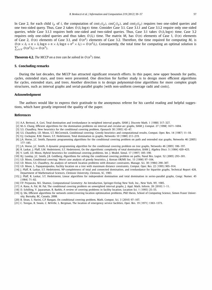
R. Benkoczi et al. / Information and Computation 219 (2012) 39–57 57
In Case 2, for each child ip of i, the computation of cost1(ip), cost′1(ip), and cost2(ip) requires two one-sided queries andone two-sided query. Thus, Case 2 takes O (δi logn) time. Consider Case 3.1. Case 3.1.1 and Case 3.1.2 require only one-sidedqueries, while Case 3.1.3 requires both one-sided and two-sided queries. Thus, Case 3.1 takes O (δi log n) time. Case 3.2requires only one-sided queries and thus takes O (δi) time. The matrix Mi has O (n) elements of Case 1, O (n) elementsof Case 2, O (n) elements of Case 3.1, and O (n2) elements of Case 3.2. Therefore, the time required for computing Mi isO (n × δi + n × δi logn + n × δi log n + n2 × δi) = O (n2δi). Consequently, the total time for computing an optimal solution is∑
i∈V O (n2δi) = O (n3).
Theorem 4.2. The MCCP on a tree can be solved in O (n3) time.
5. Concluding remarks
During the last decades, the MCCP has attracted significant research efforts. In this paper, new upper bounds for paths,cycles, extended stars, and trees were presented. One direction for further study is to design more efficient algorithmsfor cycles, extended stars, and trees. Another direction is to design polynomial-time algorithms for more complex graphstructures, such as interval graphs and serial-parallel graphs (with non-uniform coverage radii and costs).
Acknowledgment
The authors would like to express their gratitude to the anonymous referee for his careful reading and helpful sugges-tions, which have greatly improved the quality of the paper.
References
[1] A.A. Bertossi, A. Gori, Total domination and irredundance in weighted interval graphs, SIAM J. Discrete Math. 1 (1988) 317–327.[2] M.-S. Chang, Efficient algorithms for the domination problems on interval and circular-arc graphs, SIAM J. Comput. 27 (1998) 1671–1694.[3] S.S. Chaudhry, New heuristics for the conditional covering problem, Opsearch 30 (1993) 42–47.[4] S.S. Chaudhry, I.D. Moon, S.T. McCormick, Conditional covering: Greedy heuristics and computational results, Comput. Oper. Res. 14 (1987) 11–18.[5] E.J. Cockayne, R.M. Dawes, S.T. Hedetniemi, Total domination in graphs, Networks 10 (1980) 211–219.[6] J.A. Horne, J.C. Smith, Dynamic programming algorithms for the conditional covering problem on path and extended star graphs, Networks 46 (2005)
177–185.[7] J.A. Horne, J.C. Smith, A dynamic programming algorithm for the conditional covering problem on tree graphs, Networks 46 (2005) 186–197.[8] R. Laskar, J. Pfaff, S.M. Hedetniemi, S.T. Hedetniemi, On the algorithmic complexity of total domination, SIAM J. Algebra Discr. 5 (1984) 420–425.[9] V. Lotfi, I.D. Moon, Hybrid heuristics for conditional covering problems, Int. J. Model. Simul. 17 (1997) 185–190.
[10] B.J. Lunday, J.C. Smith, J.B. Goldberg, Algorithms for solving the conditional covering problem on paths, Naval Res. Logist. 52 (2005) 293–301.[11] I.D. Moon, Conditional covering: Worst case analysis of greedy heuristics, J. Korean OR/MS Soc. 15 (1990) 97–104.[12] I.D. Moon, S.S. Chaudhry, An analysis of network location problems with distance constraints, Manage. Sci. 30 (1984) 290–307.[13] I.D. Moon, L. Papayanopoulos, Facility location on a tree with maximum distance constraints, Comput. Oper. Res. 22 (1995) 905–914.[14] J. Pfaff, R. Laskar, S.T. Hedetniemi, NP-completeness of total and connected domination, and irredundance for bipartite graphs, Technical Report 428,
Department of Mathematical Sciences, Clemson University, Clemson, SC, 1983.[15] J. Pfaff, R. Laskar, S.T. Hedetniemi, Linear algorithms for independent domination and total domination in series-parallel graphs, Congr. Numer. 45
(1984) 71–82.[16] F.P. Preparata, M.I. Shamos, Computational Geometry: An Introduction, Springer-Verlag New York, Inc., New York, NY, 1985.[17] A. Rana, A. Pal, M. Pal, The conditional covering problem on unweighted interval graphs, J. Appl. Math. Inform. 28 (2010) 1–11.[18] D. Schilling, V. Jayaraman, R. Barkhi, A review of covering problems in facility location, Location Sci. 1 (1993) 25–55.[19] Q. Shi, Efficient algorithms for network center/covering location optimization problems, PhD thesis, School of Computing Science, Simon Fraser Univer-
sity, Burnaby, BC, Canada, 2008.[20] B. Sivan, S. Harini, C.P. Rangan, On conditional covering problem, Math. Comput. Sci. 3 (2010) 97–107.[21] C. Toregas, R. Swain, C. ReVelle, L. Bergman, The location of emergency service facilities, Oper. Res. 19 (1971) 1363–1373.