Embed Size (px)
Citation preview
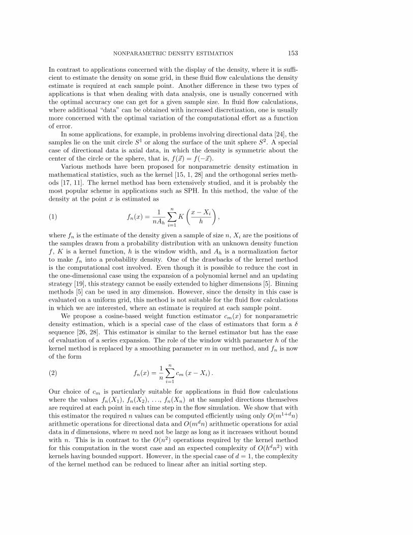
EFFICIENT NONPARAMETRIC DENSITY ESTIMATION ON THE
SPHERE WITH APPLICATIONS IN FLUID MECHANICS∗
OMER EGECIOGLU† AND ASHOK SRINIVASAN‡
SIAM J. SCI. COMPUT. c© 2000 Society for Industrial and Applied MathematicsVol. 22, No. 1, pp. 152–176
Abstract. The application of nonparametric probability density function estimation for thepurpose of data analysis is well established. More recently, such methods have been applied tofluid flow calculations since the density of the fluid plays a crucial role in determining the flow.Furthermore, when the calculations involve directional or axial data, the domain of interest falls onthe surface of the sphere. Accurate and fast estimation of probability density functions is crucial forthese calculations since the density estimation is performed at each iteration during the computation.In particular the values fn(X1), fn(X2), . . . , fn(Xn) of the density estimate at the sampled pointsXi are needed to evolve the system. Usual nonparametric estimators make use of kernel functions toconstruct fn. We propose a special sequence of weight functions for nonparametric density estimationthat is especially suitable for such applications. The resulting method has a computational advantageover kernel methods in certain situations and also parallelizes easily. Conditions for convergence turnout to be similar to those required for kernel-based methods. We also discuss experiments on differentdistributions and compare the computational efficiency of our method with kernel based estimators.
Key words. probability density, nonparametric estimation, fluid mechanics, convergence, kernelmethod, efficient algorithm
AMS subject classifications. 65U05, 62G05, 62G07, 65D15, 65Y20
PII. S1064827595290462
1. Introduction. Nonparametric density estimation is the problem of the es-timation of the values of a probability density function, given samples from the as-sociated distribution. No assumption is made about the type of the distributionfrom which the samples are drawn. This is in contrast to parametric estimationin which the density is assumed to come from a given family, and the parametersare then estimated by various statistical methods. Early contributors to the theoryof nonparametric estimation include Smirnov [21], Rosenblatt [16], Parzen [15], andChentsov [3]. Extensive descriptions of various approaches to nonparametric estima-tion along with a comprehensive bibliography can be found in books by Silverman[23] and Nadaraya [14]. More recent developments are presented in books by Scott[18] and Wand and Jones [27]. Results of the experimental comparison of some widelyused methods appear in [10, 25].
In addition to data analysis, an important application of nonparametric densityestimation is in computational fluid mechanics. When the flow calculations are per-formed in a Lagrangian framework, a set of points in space are evolved through timeusing the governing equations. In time, points that were initially close can move apart,leading to mesh distortion and numerical difficulties. Problems with mesh distortioncan be eliminated to a certain extent by the use of smoothed particle hydrodynamics(SPH) techniques [2, 13, 9, 12]. SPH treats the points being tracked as samples com-ing from an unknown probability distribution. These calculations often require thecomputation of the values of not only the unknown density, but its gradient as well.
∗Received by the editors August 16, 1995; accepted for publication (in revised form) August 3,1999; published electronically June 13, 2000.
http://www.siam.org/journals/sisc/22-1/29046.html†Department of Computer Science, University of California, Santa Barbara, CA 93106 (omer@cs.
ucsb.edu).‡Department of Mathematics, Indian Institute of Technology, Bombay, India (ashok@math.
iitb.ernet.in).
152
NONPARAMETRIC DENSITY ESTIMATION 153
In contrast to applications concerned with the display of the density, where it is suffi-cient to estimate the density on some grid, in these fluid flow calculations the densityestimate is required at each sample point. Another difference in these two types ofapplications is that when dealing with data analysis, one is usually concerned withthe optimal accuracy one can get for a given sample size. In fluid flow calculations,where additional “data” can be obtained with increased discretization, one is usuallymore concerned with the optimal variation of the computational effort as a functionof error.
In some applications, for example, in problems involving directional data [24], thesamples lie on the unit circle S1 or along the surface of the unit sphere S2. A specialcase of directional data is axial data, in which the density is symmetric about thecenter of the circle or the sphere, that is, f(�x) = f(−�x).
Various methods have been proposed for nonparametric density estimation inmathematical statistics, such as the kernel [15, 1, 28] and the orthogonal series meth-ods [17, 11]. The kernel method has been extensively studied, and it is probably themost popular scheme in applications such as SPH. In this method, the value of thedensity at the point x is estimated as
fn(x) =1
nAh
n∑
i=1
K
(
x−Xi
h
)
,(1)
where fn is the estimate of the density given a sample of size n, Xi are the positions ofthe samples drawn from a probability distribution with an unknown density functionf , K is a kernel function, h is the window width, and Ah is a normalization factorto make fn into a probability density. One of the drawbacks of the kernel methodis the computational cost involved. Even though it is possible to reduce the cost inthe one-dimensional case using the expansion of a polynomial kernel and an updatingstrategy [19], this strategy cannot be easily extended to higher dimensions [5]. Binningmethods [5] can be used in any dimension. However, since the density in this case isevaluated on a uniform grid, this method is not suitable for the fluid flow calculationsin which we are interested, where an estimate is required at each sample point.
We propose a cosine-based weight function estimator cm(x) for nonparametricdensity estimation, which is a special case of the class of estimators that form a δsequence [26, 28]. This estimator is similar to the kernel estimator but has the easeof evaluation of a series expansion. The role of the window width parameter h of thekernel method is replaced by a smoothing parameter m in our method, and fn is nowof the form
fn(x) =1
n
n∑
i=1
cm (x−Xi) .(2)
Our choice of cm is particularly suitable for applications in fluid flow calculationswhere the values fn(X1), fn(X2), . . ., fn(Xn) at the sampled directions themselvesare required at each point in each time step in the flow simulation. We show that withthis estimator the required n values can be computed efficiently using only O(m1+dn)arithmetic operations for directional data and O(mdn) arithmetic operations for axialdata in d dimensions, where m need not be large as long as it increases without boundwith n. This is in contrast to the O(n2) operations required by the kernel methodfor this computation in the worst case and an expected complexity of O(hdn2) withkernels having bounded support. However, in the special case of d = 1, the complexityof the kernel method can be reduced to linear after an initial sorting step.
154 OMER EGECIOGLU AND ASHOK SRINIVASAN
We derive conditions under which the sequence of estimated density functions fnconstructed in this fashion converge to the unknown density f , and experimentallyverify the accuracy and the efficiency of our method in practical test cases. Exper-iments and theoretical analyses also indicate how m should vary with n for optimalaccuracy.
The paper is organized as follows. In section 2 we define the weight functionestimator cm and give the conditions for the convergence of the mean integrated squareerror (MISE) when the sample space is S1 (Theorem 3). The conditions guaranteethat
∫
E(fn(x) − f(x))2dx → 0
as n → ∞. We also present corresponding results for S2. In section 3 schemes forefficient computation of these estimates on S1 and S2 are presented. In sections 4and 5, we describe experimental results with our estimator and compare it with thekernel method for some distributions encountered in practice. Our experiments implya net savings on the number of operations performed over kernel methods in certainsituations and also verify the formula found for the optimal choice of m. The resultsshow that the kernel method and our estimator perform well in different settings, andthus complement each other. The main conclusions are presented in section 6. Theappendix contains additional test results.
2. The cosine estimator and the convergence of MISE. In this section, wefirst mention some related work done on spherical data; then we define our estimatorand derive conditions for its convergence for directional data on the circle, and givecorresponding results for directional and axial data on the sphere and axial data onthe circle.
The kernel method for nonparametric density estimation for directional and axialdata is discussed in [6, 8]. While dealing with directional data, Fisher, Lewis, andEmbleton [6] recommend using the following kernel:
Wn(P, Pi) =
[
Cn
4π sinh(Cn)
]
exp[
Cn(xTXi)]
.(3)
For axial data they recommend the kernel
Wn(P, Pi) = A(Cn) exp[
Cn(xTXi)]
,(4)
where A(Cn) normalizes W to a probability density function, and Cn is the reciprocalof h used in the definition of kernel estimators. x and Xi are the Cartesian represen-tation of points P and Pi, respectively, and xTXi is the inner product of these twovectors. Wn(P, Pi) plays the role of K(x − Xi) of (1). Hall, Watson, and Cabrera[8] analyze estimators for directional data with the x − Xi term in (1) replaced by1 − xTXi. Observe that the term xTXi is the cosine of the angle between the pointsP and Pi, and therefore 1 − xTXi is a measure of the distance along the surfaceof the sphere between points P and Pi. Inner product plays a crucial role in theseestimators. We consider an estimator that can be written in terms of powers of theinner product, the power playing the role of the smoothing parameter. This enablesus to expand the estimator in a series and facilitates fast computation.
NONPARAMETRIC DENSITY ESTIMATION 155
/4π
/4)πc (x-
/4π c (x) /4)πc (x-
π π
O
O
c (x)32
32 32
(a) (b)
-
32
x
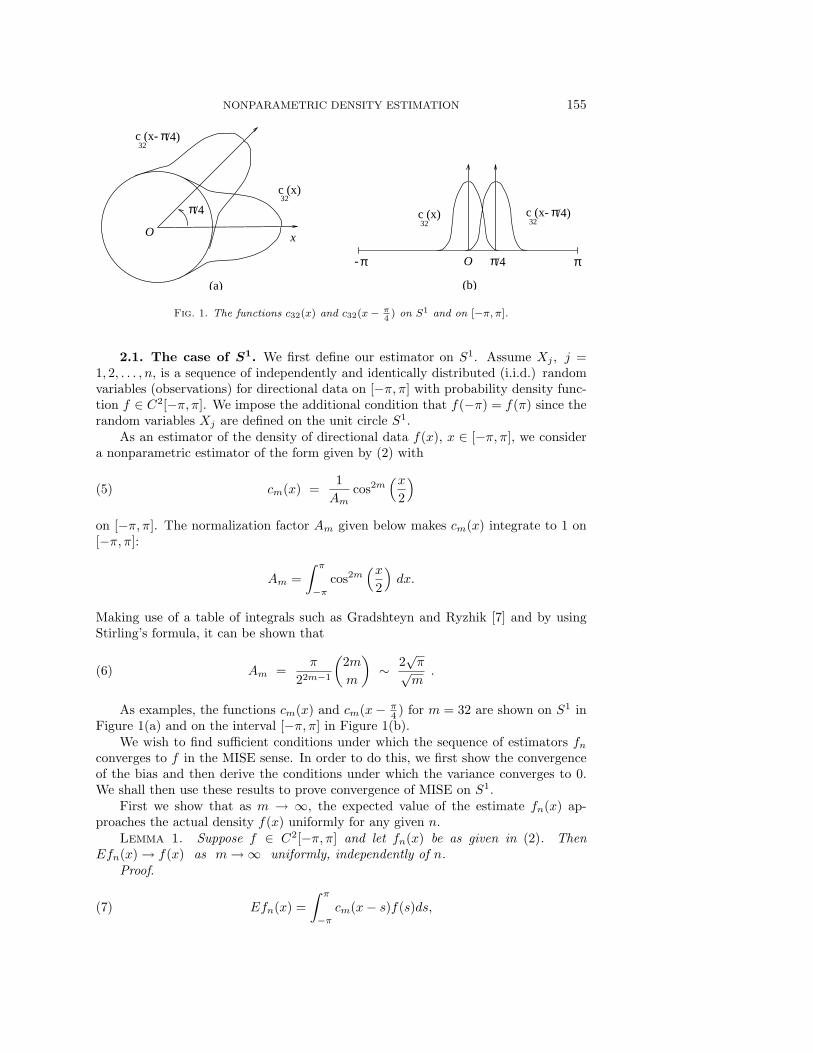
Fig. 1. The functions c32(x) and c32(x−π4) on S1 and on [−π, π].
2.1. The case of S1. We first define our estimator on S1. Assume Xj , j =
1, 2, . . . , n, is a sequence of independently and identically distributed (i.i.d.) randomvariables (observations) for directional data on [−π, π] with probability density func-tion f ∈ C2[−π, π]. We impose the additional condition that f(−π) = f(π) since therandom variables Xj are defined on the unit circle S1.
As an estimator of the density of directional data f(x), x ∈ [−π, π], we considera nonparametric estimator of the form given by (2) with
cm(x) =1
Amcos2m
(x
2
)
(5)
on [−π, π]. The normalization factor Am given below makes cm(x) integrate to 1 on[−π, π]:
Am =
∫ π
−π
cos2m(x
2
)
dx.
Making use of a table of integrals such as Gradshteyn and Ryzhik [7] and by usingStirling’s formula, it can be shown that
Am =π
22m−1
(
2m
m
)
∼ 2√π√m
.(6)
As examples, the functions cm(x) and cm(x− π4 ) for m = 32 are shown on S1 in
Figure 1(a) and on the interval [−π, π] in Figure 1(b).We wish to find sufficient conditions under which the sequence of estimators fn
converges to f in the MISE sense. In order to do this, we first show the convergenceof the bias and then derive the conditions under which the variance converges to 0.We shall then use these results to prove convergence of MISE on S1.
First we show that as m → ∞, the expected value of the estimate fn(x) ap-proaches the actual density f(x) uniformly for any given n.Lemma 1. Suppose f ∈ C2[−π, π] and let fn(x) be as given in (2). Then
Efn(x) → f(x) as m → ∞ uniformly, independently of n.
Proof.
Efn(x) =
∫ π
−π
cm(x− s)f(s)ds,(7)
156 OMER EGECIOGLU AND ASHOK SRINIVASAN
as shown in Silverman [20] and Whittle [29]. By a change of variable
∫ π
−π
cm(x− s)f(s)ds =
∫ x+π
x−π
cm(−y)f(x + y)dy =
∫ x+π
x−π
cm(y)f(x + y)dy(8)
since cm(y) = cm(−y). By using the periodicity of cm and f , along with (7), (8), andthe mean value theorem,
Efn(x) =
∫ π
−π
cm(y)f(x + y)dy =
∫ π
−π
cm(y)(f(x) + f ′(x)y + f ′′(ξx(y))y2/2)dy,
where ξx(y) is some point between x and y. Therefore
Efn(x) = f(x)
∫ π
−π
cm(y)dy +
∫ π
−π
cm(y)f ′(x)ydy +
∫ π
−π
cm(y)f ′′(ξx(y))y2/2dy.
From (6), the first integral evaluates to 1, and since ycm(y) is an odd function, thesecond integral evaluates to 0. Let 2M ′ = maxx∈[−π,π] |f ′′(x)|. We then have thefollowing estimate for the bias:
|Efn(x) − f(x)| ≤∣
∣
∣
∣
∫ π
−π
cm(y)f ′′(ξx(y))y2dy
∣
∣
∣
∣
≤ M ′
∫ π
−π
cm(y)y2dy = M ′
∫ π
−π
1
Amcos2m(y/2)y2dy.
For any δ such that 0 < δ ≤ π,
|Efn(x) − f(x)| ≤ M ′
∫
|y|<δ
1
Amcos2m(y/2)y2dy + M ′
∫
|y|≥δ
1
Amcos2m(y/2)y2dy
≤ M ′δ2
∫
|y|<δ
1
Amcos2m(y/2)dy +
2π3M ′
3
1
Amcos2m(δ/2)(9)
since cos y decreases as |y| increases on the interval under consideration. Furthermore,the integral in (9) is bounded above by 1. Therefore,
|Efn(x) − f(x)| ≤ M ′δ2 +2π3M ′
3
cos2m(δ/2)
Am
≤ M ′δ2 +2π3M ′
3
(
1 − δ2/8 + δ4/384)2m
Am(10)
= M ′δ2 +2π3M ′
3
(
1 − δ2(1 − δ2/48)/8)2m
Am.
In order to get a bound, we will choose δ as a function of m. If we take δ → 0
as m → ∞, then(
1 − δ2(1 − δ2/48)/8)2m → exp(−mδ2(1 − δ2/48)/4). Observe
that if mδ2 → ∞ as m → ∞, then this term decays exponentially. The secondexpression in (10) is the product of this term and 1/Am = O(
√m), and thus the
product approaches 0 since the exponential decay dominates. In order to get a goodbound on the first term of (10), we wish to choose δ satisfying the condition that
mδ2 → ∞ such that the δ2 is as small as possible. We can choose δ = 1/m12−ǫ,
where ǫ > 0 is arbitrarily small. Thus M ′/m is an asymptotic bound on the bias.Furthermore, the bound is independent of x; hence, the convergence is uniform.
NONPARAMETRIC DENSITY ESTIMATION 157
Lemma 2. Suppose f ∈ C2[−π, π] and let fn(x) be as given in (2). Then
var fn(x) → 0 uniformly as n → ∞, provided m → ∞ as n → ∞, and m = o(n2).Proof.
var fn(x) =1
n
∫ π
−π
cm(x− s)2f(s)ds− 1
n
{∫ π
−π
cm(x− s)f(s)ds
}2
as shown in Whittle [29]. As a consequence of Lemma 1, the second integral ap-proaches f(x) asymptotically, and hence, the second term approach 0 since f isbounded. It thus suffices to show the convergence of the first integral to 0.
Let M = maxx∈[−π,π] |f(x)|. As in Lemma 1, making a change of variable y =x− s and using periodicity as in (8), we get
1
n
∫ π
−π
cm(y)2f(x + y)dy ≤ MA2m
nA2m
→ M√8π
√m
n,
where the expression on the right-hand side is a consequence of the asymptotic ex-pression for Am in (6). Since m/n2 → 0 as n → ∞, the above integral converges to0. Since m is independent of x, the convergence is uniform. Therefore the variance offn(x) converges uniformly to 0 under the conditions of the lemma.
Note that the bound on the bias for the cosine method given by Lemma 1 is ofthe form
|Efn(x) − f(x)| ≤ 1
2max |f ′′(x)|/m,(11)
and the bound for the variance given by Lemma 2 is
var fn(x) ≤ 1√8π
max |f(x)|√m/n .(12)
Therefore, the role played by m for the cosine method is the same as h−2 of the kernelbased methods, where h is the window width of the kernel estimator. In other wordswhen m ∼ h−2, the bounds on the bias and the variance of the cosine estimator are inaccordance with the asymptotic behavior of the kernel method found in Silverman [23].Such similarity of rates of convergence is to be expected since the cosine estimator isessentially like the kernel estimator, though the forms of the functions differ. It will beshown later that the main advantage of the cosine estimator lies in its computationalefficiency.Theorem 3. Suppose f ∈ C2[−π, π] and fn(x) is as given in (2). If m → ∞ as
n → ∞, and m = o(n2), then
MISE =
∫ π
−π
E(fn(x) − f(x))2dx → 0
as n → ∞.
Proof.
∫
E(fn(x) − f(x))2dx =
∫
(Efn(x) − f(x))2dx +
∫
var fn(x)dx
as shown in Whittle [29]. From Lemmas 1 and 2, each of the integrals approaches 0.Hence, the MISE converges to 0.
158 OMER EGECIOGLU AND ASHOK SRINIVASAN
In fact, the MISE is of the form
MISE = O(1/m2) + O(√m/n),(13)
where the asymptotic bounds on the constants are as given in (11) and (12). However,as we shall explain later, the exact asymptotic constants are not all that importantfor practical computations.
Conditions for the convergence of the estimates and its derivatives on the realline instead of S1 can be found in [4]. Next we consider the case when the directionaldata lie along the surface of the unit sphere.
2.2. The case of S2. Let Xj , j = 1, 2, . . . , n, be a sequence of i.i.d. random
variables (observations) with values on the surface of the unit sphere S2 centered atthe origin in R
3. Suppose that the probability density function f(x) of the Xj hasbounded second derivatives. We consider a nonparametric estimator of the form
fn(x) =1
n
n∑
i=1
cm(x,Xi)(14)
for some m to be determined as a function of n. The cm are defined in this case asfollows. If αxX denotes the angle between points x and X, then
cm(x,X) =1
Amcos2m
(αxX
2
)
.(15)
The normalizing factor Am is given below:
Am =4π
m + 1.
Through a derivation along the lines of the case of the circle, the following theoremcan be proved for the convergence of the estimators.Theorem 4. Suppose f ∈ C2(S2) and let fn(x) be as given in (14). If m → ∞
as n → ∞ and m = o(n), then
MISE =
∫
E(fn(x) − f(x))2dx → 0.
Analogous to (13), the form of the MISE is found to be
MISE = O
(
1
m2
)
+ O(m
n
)
.(16)
From this expression for MISE we see that as in the case of S1, m ∼ h−2, where h isthe window width of the kernel estimator.
When dealing with axial data, we can consider the following axial estimator forspherical data:
cm(x,X) =1
A2mcos2m(αxX).
We can also define a corresponding estimator on the circle, where we take the cosineof the arc length between two points, instead of the cosine of half the arc length as inthe case of directional data. The relationship between the asymptotic MISE, m and n,is the same as in (13) and (16) for the cases of the circle and the sphere, respectively.
NONPARAMETRIC DENSITY ESTIMATION 159
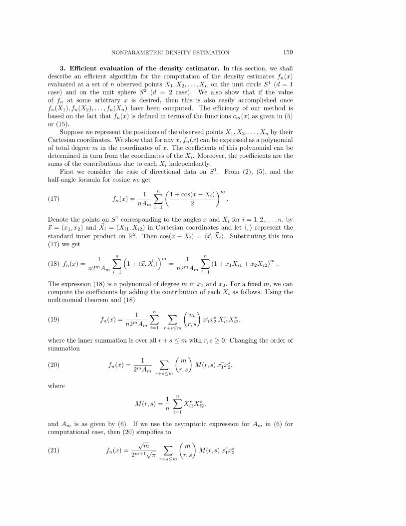
3. Efficient evaluation of the density estimator. In this section, we shalldescribe an efficient algorithm for the computation of the density estimates fn(x)evaluated at a set of n observed points X1, X2, . . . , Xn on the unit circle S1 (d = 1case) and on the unit sphere S2 (d = 2 case). We also show that if the valueof fn at some arbitrary x is desired, then this is also easily accomplished oncefn(X1), fn(X2), . . . , fn(Xn) have been computed. The efficiency of our method isbased on the fact that fn(x) is defined in terms of the functions cm(x) as given in (5)or (15).
Suppose we represent the positions of the observed points X1, X2, . . . , Xn by theirCartesian coordinates. We show that for any x, fn(x) can be expressed as a polynomialof total degree m in the coordinates of x. The coefficients of this polynomial can bedetermined in turn from the coordinates of the Xi. Moreover, the coefficients are thesums of the contributions due to each Xi independently.
First we consider the case of directional data on S1. From (2), (5), and thehalf-angle formula for cosine we get
fn(x) =1
nAm
n∑
i=1
(
1 + cos(x−Xi)
2
)m
.(17)
Denote the points on S1 corresponding to the angles x and Xi for i = 1, 2, . . . , n, by�x = (x1, x2) and �Xi = (Xi1, Xi2) in Cartesian coordinates and let 〈, 〉 represent the
standard inner product on R2. Then cos(x − Xi) = 〈�x, �Xi〉. Substituting this into
(17) we get
fn(x) =1
n2mAm
n∑
i=1
(
1 + 〈�x, �Xi〉)m
=1
n2mAm
n∑
i=1
(1 + x1Xi1 + x2Xi2)m.(18)
The expression (18) is a polynomial of degree m in x1 and x2. For a fixed m, we cancompute the coefficients by adding the contribution of each Xi as follows. Using themultinomial theorem and (18)
fn(x) =1
n2mAm
n∑
i=1
∑
r+s≤m
(
m
r, s
)
xr1x
s2 X
ri1X
si2,(19)
where the inner summation is over all r + s ≤ m with r, s ≥ 0. Changing the order ofsummation
fn(x) =1
2mAm
∑
r+s≤m
(
m
r, s
)
M(r, s) xr1x
s2,(20)
where
M(r, s) =1
n
n∑
i=1
Xri1X
si2,
and Am is as given by (6). If we use the asymptotic expression for Am in (6) forcomputational ease, then (20) simplifies to
fn(x) =
√m
2m+1√π
∑
r+s≤m
(
m
r, s
)
M(r, s) xr1x
s2(21)
160 OMER EGECIOGLU AND ASHOK SRINIVASAN
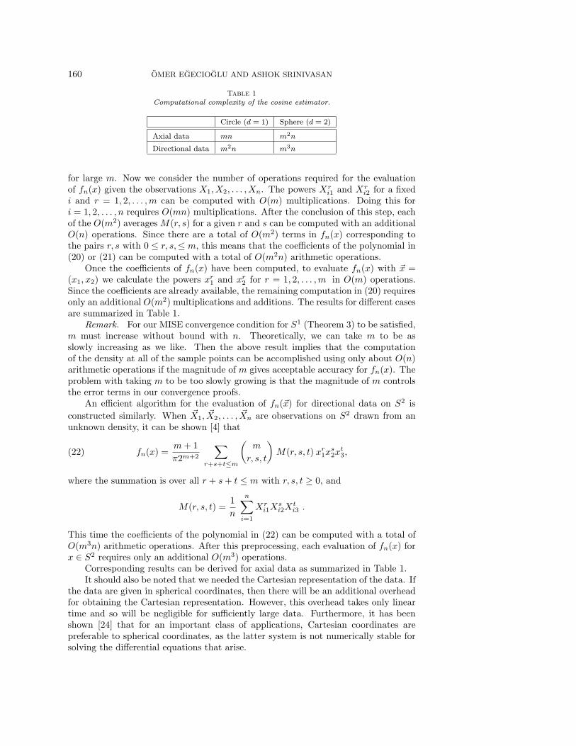
Table 1
Computational complexity of the cosine estimator.
Circle (d = 1) Sphere (d = 2)
Axial data mn m2n
Directional data m2n m3n
for large m. Now we consider the number of operations required for the evaluationof fn(x) given the observations X1, X2, . . . , Xn. The powers Xr
i1 and Xri2 for a fixed
i and r = 1, 2, . . . ,m can be computed with O(m) multiplications. Doing this fori = 1, 2, . . . , n requires O(mn) multiplications. After the conclusion of this step, eachof the O(m2) averages M(r, s) for a given r and s can be computed with an additionalO(n) operations. Since there are a total of O(m2) terms in fn(x) corresponding tothe pairs r, s with 0 ≤ r, s,≤ m, this means that the coefficients of the polynomial in(20) or (21) can be computed with a total of O(m2n) arithmetic operations.
Once the coefficients of fn(x) have been computed, to evaluate fn(x) with �x =(x1, x2) we calculate the powers xr
1 and xr2 for r = 1, 2, . . . ,m in O(m) operations.
Since the coefficients are already available, the remaining computation in (20) requiresonly an additional O(m2) multiplications and additions. The results for different casesare summarized in Table 1.
Remark. For our MISE convergence condition for S1 (Theorem 3) to be satisfied,m must increase without bound with n. Theoretically, we can take m to be asslowly increasing as we like. Then the above result implies that the computationof the density at all of the sample points can be accomplished using only about O(n)arithmetic operations if the magnitude of m gives acceptable accuracy for fn(x). Theproblem with taking m to be too slowly growing is that the magnitude of m controlsthe error terms in our convergence proofs.
An efficient algorithm for the evaluation of fn(�x) for directional data on S2 is
constructed similarly. When �X1, �X2, . . . , �Xn are observations on S2 drawn from anunknown density, it can be shown [4] that
fn(x) =m + 1
π2m+2
∑
r+s+t≤m
(
m
r, s, t
)
M(r, s, t) xr1x
s2x
t3,(22)
where the summation is over all r + s + t ≤ m with r, s, t ≥ 0, and
M(r, s, t) =1
n
n∑
i=1
Xri1X
si2X
ti3 .
This time the coefficients of the polynomial in (22) can be computed with a total ofO(m3n) arithmetic operations. After this preprocessing, each evaluation of fn(x) forx ∈ S2 requires only an additional O(m3) operations.
Corresponding results can be derived for axial data as summarized in Table 1.It should also be noted that we needed the Cartesian representation of the data. If
the data are given in spherical coordinates, then there will be an additional overheadfor obtaining the Cartesian representation. However, this overhead takes only lineartime and so will be negligible for sufficiently large data. Furthermore, it has beenshown [24] that for an important class of applications, Cartesian coordinates arepreferable to spherical coordinates, as the latter system is not numerically stable forsolving the differential equations that arise.
NONPARAMETRIC DENSITY ESTIMATION 161
In the subsequent parts of this section we shall compare the computational effi-ciency of our scheme with that of the kernel method.
3.1. Parallelization. One of the advantages of the computational strategy de-scribed above is the ease of parallelization. Parallelization is required in many fluidflow calculations due to the large sizes of the systems. The kernel method is some-what difficult to parallelize. If we use an efficient kernel implementation that performskernel evaluations only for those points which are within a cut-off distance h of thegiven sample, then an efficient implementation of the parallelization requires periodicload balancing and domain decomposition so that points that are close by remain onthe same processor, and so that each processor has roughly the same load in termsof the computational effort. Also, the communication pattern for the kernel methodis not very regular. In contrast, parallelization for the cosine estimator can easilybe accomplished by a global reduction operation, for which efficient implementationsare usually available. This method requires the same computational effort for eachpoint, and so the load is easily balanced by having the same number of points in eachprocessor. Domain decomposition does not play an important role in this scheme,since the points can be on any processor.
3.2. Theoretical comparison of the kernel and the cosine estimators.
Now we analyze the computational efficiency of the kernel and the cosine densityestimation methods. An important measure of the efficiency of the algorithms is notjust the convergence rate of the error with sample size n, but the relationship of thecomputational effort C required as a function of the error E. For the kernel estimator,we can write the asymptotic MISE E as
E = O
(
h4 +1
hdn
)
,(23)
where h is the smoothing parameter, d = 1, 2 is the dimension, and n is the samplesize. The computational effort required for this nonparametric density estimation canbe expressed as
C = O(hβnγ),(24)
where 0 ≤ β ≤ d and γ = 1 or 2 depending on the details of the algorithm used. Fora given sample size, (23) gives the optimal h as h ∼ n−1/(d+4). However, since theequation for the computational complexity also depends on h, we need to considerthe possibility that a value of h smaller than this optimal value may actually resultin a lower computational effort.
Let us consider a variation of h with n of the form
h = O(n−α), 1/(d + 4) ≤ α < 1/d .(25)
From (25), (24), and (23) we obtain
C = n−αβ+γ ⇒ n = C1
γ−βα ⇒ E = C−4αγ−βα + C
dα−1γ−βα .
For minimum error, the exponent of both the terms on the right should be the same,otherwise the error due to the higher term will dominate. This leads to α = 1/(d + 4)which is the same as the value of optimal α for a given n. If we let hoptn representthe optimal h minimizing the MISE for a given n, and hoptC represent the optimal
162 OMER EGECIOGLU AND ASHOK SRINIVASAN
h minimizing the computational effort as a function of the error, then the expressionderived above for α does not necessarily imply that hoptn = hoptC since the relationhoptn = khoptC would still satisfy the expression for α for some constant k. If k < 1,then we can choose a suboptimal value of h in order to improve the speed of thealgorithm.
The optimal variation of error with computational complexity using this value ofα is given by
C = Eβ4 −
(d+4)γ4 .
Let us now consider the cosine estimator. We can write the asymptotic MISE asfollows:
E = O
(
m−2 +md/2
n
)
where E is the MISE, m is the smoothing parameter, d is the dimension (d = 1 forthe circle and d = 2 for the sphere), and n is the sample size. The computationaleffort required for this estimator can be expressed as C = O(mξn), where ξ can bedetermined from Table 1. The expression for C above is the same as (24) with γ = 1,and β = −2ξ, recalling that m behaves as h−2. By an analysis similar to the previouscase we can show that the optimal variation of error with computational complexityis given by
C = E−(d/2+ξ)
2 −1.
As examples, for the cosine estimator on the circle (d = 1) with axial data (ξ = 1)and directional data (ξ = 2), the computational complexity and the error are relatedby C = E−1.75 and C = E−2.25, respectively.
The complexity of the kernel estimator is the same for axial and directional data.However, several different possibilities exist depending on how efficient the implemen-tation of the estimator is. If we consider estimators of the form given by (3) and (4),then we have d = 1, β = 0, γ = 2, and therefore
C = E−2.5.(26)
However, if we consider a kernel with bounded support, and use an efficient imple-mentation of the algorithm that computes the kernel only for those points that havea nonzero contribution, then the expected value of β is 1 and we get C = E−2.25
for data on the circle. Note that the worst case complexity remains as in (26). Forthe d = 1 case, we can consider an efficient algorithm using polynomial kernels andupdating [19], which uses a linear time after an initial O(n log n) sorting step. Inthis case β = 0, γ = 1, and C = E−1.25, which means that the kernel method has abetter asymptotic complexity than the cosine kernel. However there appears to be nonatural generalization of this update strategy to higher dimensions [5].
Results for the different cases can be determined in the manner demonstratedabove and are presented in Table 2. We wish to mention that the exact asymptoticconstants in Theorem 3 are not quite that important (compared with the exponenton E), since asymptotically the slowdown incurred by the cache misses dominates theoverall running time. We can expect that the simpler memory access pattern of ourestimator will make it advantageous over the kernel method in the asymptotic case.
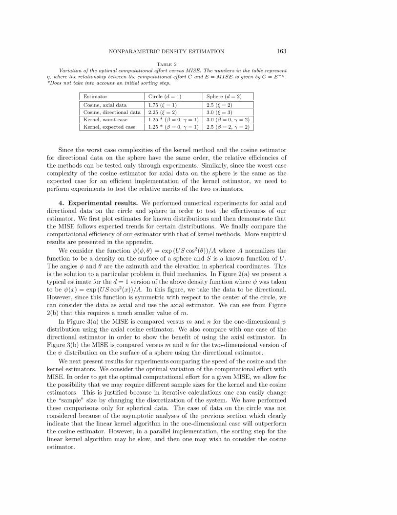
NONPARAMETRIC DENSITY ESTIMATION 163
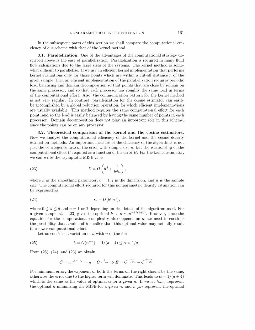
Table 2
Variation of the optimal computational effort versus MISE. The numbers in the table representη, where the relationship between the computational effort C and E = MISE is given by C = E−η.*Does not take into account an initial sorting step.
Estimator Circle (d = 1) Sphere (d = 2)
Cosine, axial data 1.75 (ξ = 1) 2.5 (ξ = 2)
Cosine, directional data 2.25 (ξ = 2) 3.0 (ξ = 3)
Kernel, worst case 1.25 * (β = 0, γ = 1) 3.0 (β = 0, γ = 2)
Kernel, expected case 1.25 * (β = 0, γ = 1) 2.5 (β = 2, γ = 2)
Since the worst case complexities of the kernel method and the cosine estimatorfor directional data on the sphere have the same order, the relative efficiencies ofthe methods can be tested only through experiments. Similarly, since the worst casecomplexity of the cosine estimator for axial data on the sphere is the same as theexpected case for an efficient implementation of the kernel estimator, we need toperform experiments to test the relative merits of the two estimators.
4. Experimental results. We performed numerical experiments for axial anddirectional data on the circle and sphere in order to test the effectiveness of ourestimator. We first plot estimates for known distributions and then demonstrate thatthe MISE follows expected trends for certain distributions. We finally compare thecomputational efficiency of our estimator with that of kernel methods. More empiricalresults are presented in the appendix.
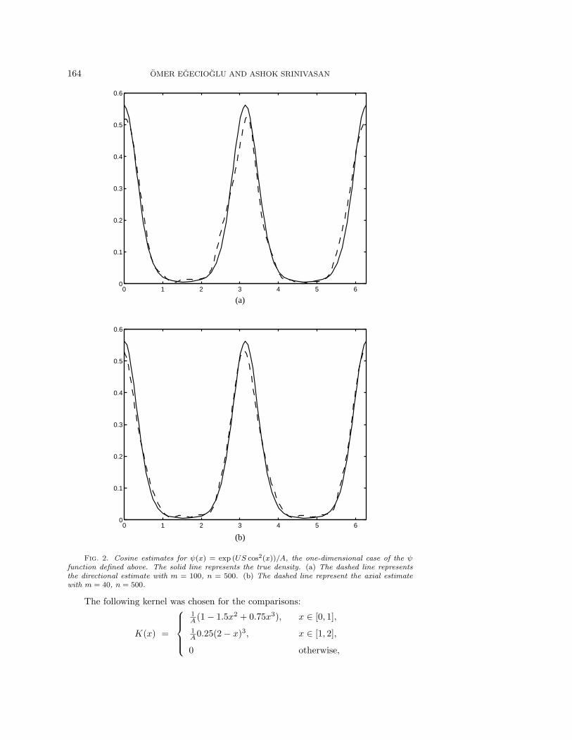
We consider the function ψ(φ, θ) = exp (US cos2(θ))/A where A normalizes thefunction to be a density on the surface of a sphere and S is a known function of U .The angles φ and θ are the azimuth and the elevation in spherical coordinates. Thisis the solution to a particular problem in fluid mechanics. In Figure 2(a) we present atypical estimate for the d = 1 version of the above density function where ψ was takento be ψ(x) = exp (US cos2(x))/A. In this figure, we take the data to be directional.However, since this function is symmetric with respect to the center of the circle, wecan consider the data as axial and use the axial estimator. We can see from Figure2(b) that this requires a much smaller value of m.
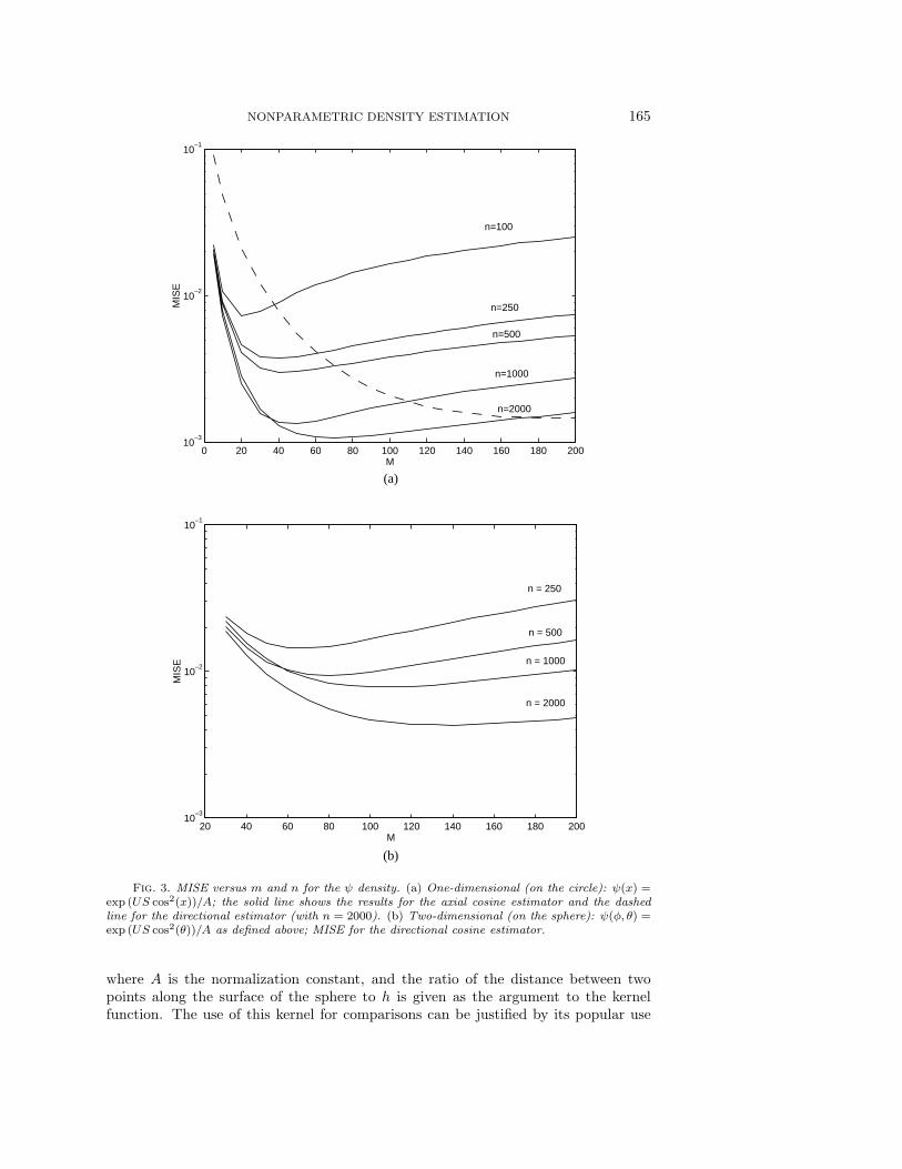
In Figure 3(a) the MISE is compared versus m and n for the one-dimensional ψdistribution using the axial cosine estimator. We also compare with one case of thedirectional estimator in order to show the benefit of using the axial estimator. InFigure 3(b) the MISE is compared versus m and n for the two-dimensional version ofthe ψ distribution on the surface of a sphere using the directional estimator.
We next present results for experiments comparing the speed of the cosine and thekernel estimators. We consider the optimal variation of the computational effort withMISE. In order to get the optimal computational effort for a given MISE, we allow forthe possibility that we may require different sample sizes for the kernel and the cosineestimators. This is justified because in iterative calculations one can easily changethe “sample” size by changing the discretization of the system. We have performedthese comparisons only for spherical data. The case of data on the circle was notconsidered because of the asymptotic analyses of the previous section which clearlyindicate that the linear kernel algorithm in the one-dimensional case will outperformthe cosine estimator. However, in a parallel implementation, the sorting step for thelinear kernel algorithm may be slow, and then one may wish to consider the cosineestimator.
164 OMER EGECIOGLU AND ASHOK SRINIVASAN
0 1 2 3 4 5 60
0.1
0.2
0.3
0.4
0.5
0.6
0 1 2 3
(a)
(b)
4 5 60
0.1
0.2
0.3
0.4
0.5
0.6
Fig. 2. Cosine estimates for ψ(x) = exp (US cos2(x))/A, the one-dimensional case of the ψfunction defined above. The solid line represents the true density. (a) The dashed line representsthe directional estimate with m = 100, n = 500. (b) The dashed line represent the axial estimatewith m = 40, n = 500.
The following kernel was chosen for the comparisons:
K(x) =
1A (1 − 1.5x2 + 0.75x3), x ∈ [0, 1],
1A0.25(2 − x)3, x ∈ [1, 2],
0 otherwise,
NONPARAMETRIC DENSITY ESTIMATION 165
20 40 60 80 100 120 140 160 180 20010
–3
10–2
10–1
M
MIS
E
n = 250
n = 500
n = 1000
n = 2000
0 20 40 60 80 100 120 140 160 180 20010
–3
10–2
10–1
M
(a)
(b)
MIS
E
n=100
n=250
n=500
n=1000
n=2000
Fig. 3. MISE versus m and n for the ψ density. (a) One-dimensional (on the circle): ψ(x) =exp (US cos2(x))/A; the solid line shows the results for the axial cosine estimator and the dashedline for the directional estimator (with n = 2000). (b) Two-dimensional (on the sphere): ψ(φ, θ) =exp (US cos2(θ))/A as defined above; MISE for the directional cosine estimator.
where A is the normalization constant, and the ratio of the distance between twopoints along the surface of the sphere to h is given as the argument to the kernelfunction. The use of this kernel for comparisons can be justified by its popular use
166 OMER EGECIOGLU AND ASHOK SRINIVASAN
0.005 0.01 0.015 0.020
0.2
0.4
0.6
0.8
1
1.2
1.4
1.6
1.8
2
MISE
Tim
e
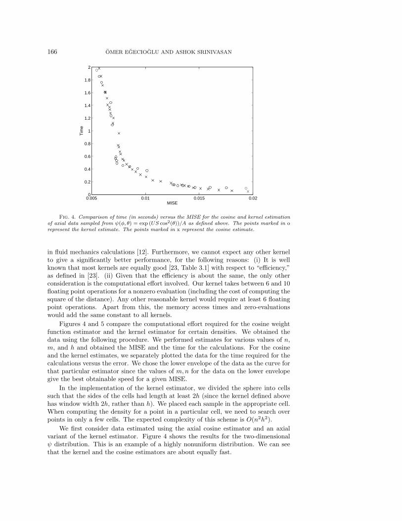
Fig. 4. Comparison of time (in seconds) versus the MISE for the cosine and kernel estimationof axial data sampled from ψ(φ, θ) = exp (US cos2(θ))/A as defined above. The points marked in orepresent the kernel estimate. The points marked in x represent the cosine estimate.
in fluid mechanics calculations [12]. Furthermore, we cannot expect any other kernelto give a significantly better performance, for the following reasons: (i) It is wellknown that most kernels are equally good [23, Table 3.1] with respect to “efficiency,”as defined in [23]. (ii) Given that the efficiency is about the same, the only otherconsideration is the computational effort involved. Our kernel takes between 6 and 10floating point operations for a nonzero evaluation (including the cost of computing thesquare of the distance). Any other reasonable kernel would require at least 6 floatingpoint operations. Apart from this, the memory access times and zero-evaluationswould add the same constant to all kernels.
Figures 4 and 5 compare the computational effort required for the cosine weightfunction estimator and the kernel estimator for certain densities. We obtained thedata using the following procedure. We performed estimates for various values of n,m, and h and obtained the MISE and the time for the calculations. For the cosineand the kernel estimates, we separately plotted the data for the time required for thecalculations versus the error. We chose the lower envelope of the data as the curve forthat particular estimator since the values of m,n for the data on the lower envelopegive the best obtainable speed for a given MISE.
In the implementation of the kernel estimator, we divided the sphere into cellssuch that the sides of the cells had length at least 2h (since the kernel defined abovehas window width 2h, rather than h). We placed each sample in the appropriate cell.When computing the density for a point in a particular cell, we need to search overpoints in only a few cells. The expected complexity of this scheme is O(n2h2).
We first consider data estimated using the axial cosine estimator and an axialvariant of the kernel estimator. Figure 4 shows the results for the two-dimensionalψ distribution. This is an example of a highly nonuniform distribution. We can seethat the kernel and the cosine estimators are about equally fast.
NONPARAMETRIC DENSITY ESTIMATION 167
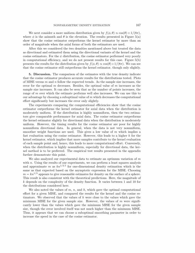
We next consider a more uniform distribution given by f(φ, θ) ∝ cos(θ) + 1/(8π),where φ is the azimuth and θ is the elevation. The results presented in Figure 5(a)show that the cosine estimator outperforms the kernel estimator by more than anorder of magnitude when the axial forms of both the estimators are used.
After this we considered the two densities mentioned above but treated the dataas directional and estimated them using the directional variants of the kernel and thecosine estimators. For the ψ distribution, the cosine estimator performed very poorlyin computational efficiency, and we do not present results for this case. Figure 5(b)presents the results for the distribution given by f(φ, θ) ∝ cos(θ)+1/(8π). We can seethat the cosine estimator still outperforms the kernel estimator, though only slightly.
5. Discussion. The comparison of the estimates with the true density indicatethat the cosine estimator produces accurate results for the distributions tested. Plotsof MISE versus m and n follow the expected trends. As the sample size increases, theerror for the optimal m decreases. Besides, the optimal value of m increases as thesample size increases. It can also be seen that as the number of points increases, therange of m over which the estimate performs well also increases. We can use this toour advantage by choosing a suboptimal value of m which decreases the computationaleffort significantly but increases the error only slightly.
The experiments comparing the computational efficiencies show that the cosineestimator outperforms the kernel estimator for axial data when the distribution ismoderately uniform. If the distribution is highly nonuniform, then the two estima-tors give comparable performance for axial data. The cosine estimator outperformsthe kernel estimator slightly for directional data when the distribution is moderatelyuniform. However, the timing results for the cosine estimator are poor for highlynonuniform directional data. In general, when the data is not very nonuniform,smoother weight functions are used. This gives a low value of m which implies afast evaluation using the cosine estimator. However, this leads to a higher h for thekernel estimator, which implies that more samples contribute to the kernel evaluationof each sample point and, hence, this leads to more computational effort. Conversely,when the distribution is highly nonuniform, especially for directional data, the ker-nel method is to be preferred. The empirical test results presented in the appendixfurther demonstrate this point.
We also analyzed our experimental data to estimate an optimum variation of mwith n. Using the results of our experiments, we can perform a least squares analysisand approximate m as kn1/2.5 for one-dimensional density estimation which is thesame as that expected based on the asymptotic expression for the MISE. Choosingm = kn1/3 appears to give reasonable estimates for density on the surface of a sphere.This result is also consistent with the theoretical predictions. Here, the magnitude ofk depends on the complexity of the density function. It varies between 1 and 10 forthe distributions considered here.
We also noted the values of m, n, and h, which gave the optimal computationaleffort for a given MISE, and compared the results for the kernel and the cosine es-timators. We observed that the values of h were close to the values which gave theminimum MISE for the given sample size. However, the values of m were signifi-cantly lower than the values which gave the minimum MISE for the given samplesize, though the error involved itself was not much higher than the minimum MISE.Thus, it appears that we can choose a suboptimal smoothing parameter in order toincrease the speed in the case of the cosine estimator.
168 OMER EGECIOGLU AND ASHOK SRINIVASAN
0.5 1 1.5 2 2.5 3 3.5 4 4.5 5
x 103
0
0.5
1
1.5
2
2.5
3
3.5
4
4.5
5
MISE
(b)
(a)
Tim
e
0.6 0.8 1 1.2 1.4 1.6 1.8 2
x 103
0
0.5
1
1.5
2
2.5
3
3.5
4
4.5
5
MISE
Tim
e
Fig. 5. Plot of time (in seconds) versus the MISE for the cosine and the kernel estimation ofdata sampled from f(φ, θ) ∝ cos(θ) + 1/(8π). The points marked in o represent the kernel estimate.The points marked in x represent the cosine estimate. (a) Data treated as axial. (b) Data treatedas directional.
NONPARAMETRIC DENSITY ESTIMATION 169
–2 –1.5 –1 –0.5 0 0.5 1 1.5 2–0.1
0
0.1
0.2
0.3
0.4
0.5
0.6
0.7
Elevation
Den
sity
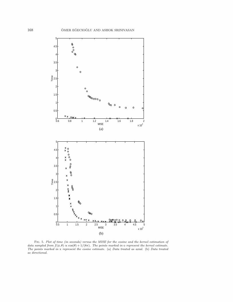
Fig. 6. Plot of density functions g(φ; s) = k cosh (s sinφ) for different values of s, where φ isthe elevation. The solid line denotes s = 8.0, the dashed line s = 4.0, the dash-dotted line s = 2.0,and the dotted line s = 0.0.
6. Conclusions. In this paper, we have described a weight function estimatorfor nonparametric estimation of probability density functions based on cosines, andwe provided conditions under which the estimate and its derivatives converge to theactual functions. We have developed a scheme for the efficient computation of thedensity and presented experimental results to check the performance of the estimatorfor practical problems. These results are particularly relevant to certain fluid mechan-ics calculations and, in general, to situations where the sample size can be controlled,for example, though refinement of the discretization. We have also given an empir-ical formula for choosing the weight function exponent parameter of the estimator.Our experimental results suggest that the cosine estimator outperforms the kernelestimator for both directional and axial data that are moderately uniform. It givesperformance comparable to the kernel estimator for highly nonuniform axial data,while the kernel method is preferable for highly nonuniform directional data. Thereis potential for further theoretical study of our estimator.
Appendix. Further test results. We present more test results in this sectionin order to study the relative efficiencies of the cosine and the kernel techniques, asthe density function is varied systematically from being relatively uniform to beingsharply peaked on the unit sphere.
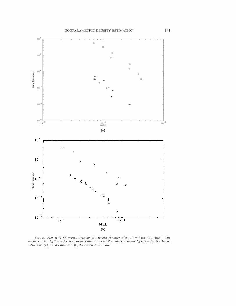
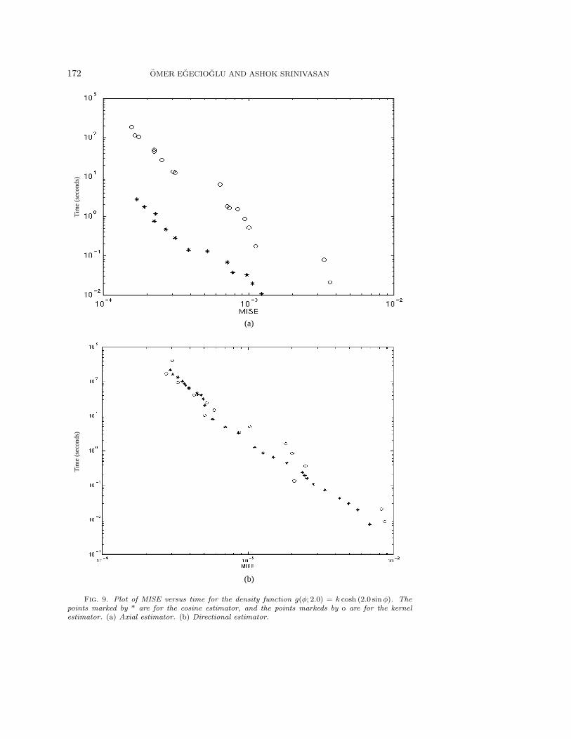
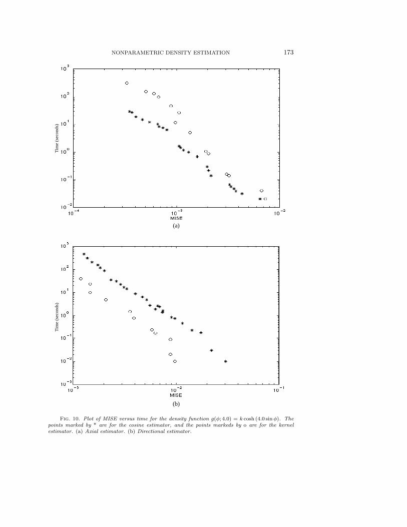
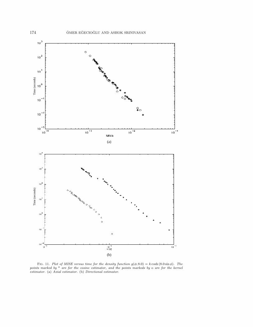
For these tests, we chose density functions g(φ; s) = k cosh (s sinφ), where s is aconstant that governs the sharpness of the density function, φ is the elevation, andk = s/(4π sinh s) normalizes this to a probability density function. Figure 6 showsthe density as a function of the elevation alone for different values of the parameter s.This function is symmetric about the center of the sphere, and thus we can use theaxial estimators, as in section 4. We can also ignore our knowledge of this symmetryand use the general directional estimators.
170 OMER EGECIOGLU AND ASHOK SRINIVASAN
(a)
(b)
Tim
e (s
econ
ds)
Tim
e (s
econ
ds)
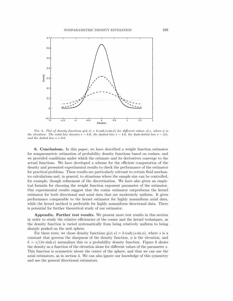
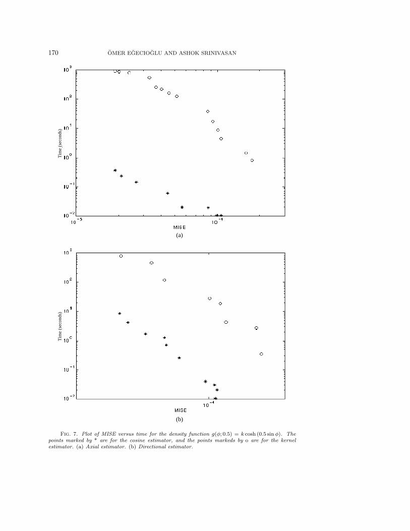
Fig. 7. Plot of MISE versus time for the density function g(φ; 0.5) = k cosh (0.5 sinφ). Thepoints marked by * are for the cosine estimator, and the points markeds by o are for the kernelestimator. (a) Axial estimator. (b) Directional estimator.
NONPARAMETRIC DENSITY ESTIMATION 171
(a)
(b)
Tim
e (s
econ
ds)
Tim
e (s
econ
ds)
Fig. 8. Plot of MISE versus time for the density function g(φ; 1.0) = k cosh (1.0 sinφ). Thepoints marked by * are for the cosine estimator, and the points markeds by o are for the kernelestimator. (a) Axial estimator. (b) Directional estimator.
172 OMER EGECIOGLU AND ASHOK SRINIVASAN
(a)
(b)
Tim
e (s
econ
ds)
Tim
e (s
econ
ds)
Fig. 9. Plot of MISE versus time for the density function g(φ; 2.0) = k cosh (2.0 sinφ). Thepoints marked by * are for the cosine estimator, and the points markeds by o are for the kernelestimator. (a) Axial estimator. (b) Directional estimator.
NONPARAMETRIC DENSITY ESTIMATION 173
(a)
(b)
Tim
e (s
econ
ds)
Tim
e (s
econ
ds)
Fig. 10. Plot of MISE versus time for the density function g(φ; 4.0) = k cosh (4.0 sinφ). Thepoints marked by * are for the cosine estimator, and the points markeds by o are for the kernelestimator. (a) Axial estimator. (b) Directional estimator.
174 OMER EGECIOGLU AND ASHOK SRINIVASANT
ime
(sec
onds
)
(a)
(b)
Tim
e (s
econ
ds)
Fig. 11. Plot of MISE versus time for the density function g(φ; 8.0) = k cosh (8.0 sinφ). Thepoints marked by * are for the cosine estimator, and the points markeds by o are for the kernelestimator. (a) Axial estimator. (b) Directional estimator.
NONPARAMETRIC DENSITY ESTIMATION 175
We present the results of the experiments as plots of time versus MISE for thekernel estimator versus the cosine estimator, for both axial and directional data. Thekernel estimator is the one used in the empirical tests in section 4. The tests wereperformed on an Intel Celeron 300MHz processor with 64 MB memory. The C codewas compiled with the gcc compiler at optimization level −O3.
We can see from Figures 7, 8, 9, 10, and 11 that when the density functionis not very sharp, the cosine estimator outperforms the kernel estimator for bothaxial and directional data. As the density becomes sharper, the kernel method startsoutperforming the cosine estimator for directional data, though the latter is stillbetter for axial data. When the density becomes extremely sharp, the kernel methodbecomes better for both types of data, though for axial data the two methods are stillcomparable to a certain extent in terms of speed. These results follow the theoreticallypredicted trends and demonstrate that these two methods complement each other fordifferent types of data.
Appendix. We thank the referees for their detailed comments and advice, espe-cially for directing our attention to the current literature.
REFERENCES
[1] P. J. Bickel and M. Rosenblatt, On some global measures of the deviations of densityfunction estimates, Ann. Stat., 1 (1973), pp. 1071–1095.
[2] C. Chaubal, O. Egecioglu, G. Leal, and A. Srinivasan, Smoothed particle hydrodynamicstechniques for the solution of kinetic theory problems. Part 1: Method, J. Non-NewtonianFluid Mech., 70 (1997), pp. 125–154.
[3] N. N. Chentsov, Estimation of unknown probability density based on observations, Dokl. Akad.Nauk SSSR, 147 (1962), pp. 45–48 (in Russian).
[4] O. Egecioglu and A. Srinivasan, Efficient Nonparametric Estimation of Probability DensityFunctions, Technical Report TRCS95-21, University of California at Santa Barbara, 1995.
[5] J. Fan and J. S. Marron, Fast implementations of nonparametric curve estimators, J. Com-put. Graph. Statist., 3 (1994), pp. 35–56.
[6] N. I. Fisher, T. Lewis, and B. J. J. Embleton, Statistical Analysis of Spherical Data, Cam-bridge University Press, Cambridge, 1993.
[7] I. S. Gradshteyn and I. M. Ryzhik, Table of Integrals, Series, and Products, Academic Press,New York, London, 1980, pp. 374.
[8] P. Hall, G. S. Watson, and J. Cabrera, Kernel density estimation with spherical data,Biometrika, 74 (1987), pp. 751–762.
[9] L. Hernquist and N. Katz, TREESPH: A unification of SPH with the hierarchical treemethod, Astrophys. J. Suppl., 70 (1989), pp. 419–446.
[10] J. Hwang, Non-parametric multivariate density estimation: A comparative study, IEEE Trans.Signal Process., 42 (1994), pp. 2795–2810.
[11] R. Kronmal and M. Tarter, The estimation of probability densities and cumulatives byFourier series methods, Amer. Statist., (1968), pp. 925–952.
[12] J. J. Monaghan and J. C. Lattanzio A refined particle method for astrophysical problems,Astron. Astrophys., 149 (1985), pp. 135–143.
[13] J. J. Monaghan, Smoothed particle hydrodynamics, Annu. Rev. Astron. Astrophys., 30 (1992),pp. 543–574.
[14] E. A. Nadaraya, Non-parametric Estimation of Probability Densities and Regression Curves,Mathematics and Applications (Soviet Series)1, Kluwer Academic Publishers, Boston,1989.
[15] E. Parzen, On estimation of a probability density function and mode, Ann. Math. Statist., 33(1962), pp. 1065–1076.
[16] M. Rosenblatt, Remarks on some non-parametric estimates of a density function, Ann. Math.Statist., 27 (1956), pp. 832–837.
[17] S. C. Schwartz, Estimation of probability density by an orthogonal series, Ann. Math. Statist.,38 (1967), pp. 1261–1265.
[18] D. W. Scott, Multivariate Density Estimation, John Wiley, New York, 1992.
176 OMER EGECIOGLU AND ASHOK SRINIVASAN
[19] B. Seifert, M. Brockmann, J. Engel, and T. Gasser, Fast algorithms for nonparametriccurve estimation, J. Comput. Graph. Statist., 3 (1994), pp. 192–213.
[20] B. W. Silverman, Kernel density estimation using the fast Fourier transform, Appl. Statist.,31 (1982), pp. 93–99.
[21] N. V. Smirnov, On the approximation of probability densities of random variables, ScholarlyNotes of Moscow State Polytechnical Institute, 16 (1951), pp. 69–96 (in Russian).
[22] G. D. Smith, Numerical Solution of Partial Differential Equations: Finite Difference Methods,Oxford University Press, London, 1978.
[23] B. W. Silverman, Density Estimation for Statistics and Data Analysis, Chapman and Hall,London, 1986.
[24] A. Szeri and L. G. Leal, A new computational method for the solution of flow problems ofmicrostructured fluids. Part 2. Inhomogeneous shear flow of a suspension, J. Fluid Mech.,262 (1994), pp. 171–204.
[25] R. Vio, G. Fasano, M. Lazzarin, and O. Lessi, Probability density estimation in astronomy,Astron. Astrophys., 289 (1994), pp. 640–648.
[26] G. Walter and J. Blum, Probability density estimation using delta sequences, Ann. Statist.,7 (1979), pp. 328–340.
[27] M. P. Wand and M. C. Jones, Kernel Smoothing, Chapman and Hall, London, 1995.[28] G. S. Watson and M. R. Leadbetter, On the estimation of the probability density, I, Ann.
Math. Statist., 34 (1963), pp. 480–491.[29] P. Whittle, On the smoothing of probability density functions, J. Roy. Statist. Soc. Ser. B, 20
(1958), pp. 334–343.