AGILE: elastic distributed resource scalingfor Infrastructure-as-a-Service

Hiep Nguyen, Zhiming Shen, Xiaohui GuNorth Carolina State University

{hcnguye3,zshen5}@ncsu.edu, gu@csc.ncsu.edu

Sethuraman SubbiahNetApp Inc.

sethu.subbiah@netapp.com

John WilkesGoogle Inc.

johnwilkes@google.com

Abstract

Dynamically adjusting the number of virtual machines(VMs) assigned to a cloud application to keep up withload changes and interference from other uses typicallyrequires detailed application knowledge and an ability toknow the future, neither of which are readily availableto infrastructure service providers or application owners.The result is that systems need to be over-provisioned(costly), or risk missing their performance Service LevelObjectives (SLOs) and have to pay penalties (alsocostly). AGILE deals with both issues: it uses waveletsto provide a medium-term resource demand predictionwith enough lead time to start up new application serverinstances before performance falls short, and it usesdynamic VM cloning to reduce application startup times.Tests using RUBiS and Google cluster traces show thatAGILE can predict varying resource demands over themedium-term with up to 3.42× better true positive rateand 0.34× the false positive rate than existing schemes.Given a target SLO violation rate, AGILE can efficientlyhandle dynamic application workloads, reducing bothpenalties and user dissatisfaction.

1 Introduction

Elastic resource provisioning is one of the most attractivefeatures provided by Infrastructure as a Service (IaaS)clouds [2]. Unfortunately, deciding when to get moreresources, and how many to get, is hard in the face ofdynamically-changingapplication workloads and servicelevel objectives (SLOs) that need to be met. Existingcommercial IaaS clouds such as Amazon EC2 [2] de-pend on the user to specify the conditions for addingor removing servers. However, workload changes andinterference from other co-located applications make thisdifficult.

Previous work [19, 39] has proposed prediction-drivenresource scaling schemes for adjusting how many re-

Host

VM +

application

VM controller

Linux + KVM

Resource

pressure

modeling

AGILE slaveResource

demand

predictionResource

monitoring

Server addition/

removal

AGILE master

Server pool

prediction

Server pool scaling

manager

Figure 1: The overall structure of the AGILE system. TheAGILE slave continuously monitors the resource usage ofdifferent servers running inside local VMs. The AGILE mastercollects the monitor data to predict future resource demands.The AGILE master maintains a dynamic resource pressuremodel for each application using online profiling. We use theterm server poolto refer to the set of application VMs thatprovide the same replicated service. Based on the resourcedemand prediction result and the resource pressure model,the AGILE master invokes the server pool manager to add orremove servers.

sources to give to an application within a single host.But distributed resource scaling (e.g., adding or remov-ing servers) is more difficult because of the latenciesinvolved. For example, the mean instantiation latencyin Amazon EC2 is around 2 minutes [8], and it may thentake a while for the new server instance to warm up: inour experiments, it takes another 2 minutes for a Cassan-dra server [4] to reach its maximum throughput. Thus,it is insufficient to apply previous short-term (i.e., lessthan a minute) prediction techniques to the distributedresource scaling system.

In this paper, we present our solution: AGILE, apractical elastic distributed resource scaling system forIaaS cloud infrastructures. Figure 1 shows its overallstructure. AGILE provides medium-term resource de-mand predictions for achieving enough time to scale upthe server pool before the application SLO is affected bythe increasing workload. AGILE leverages pre-copy live

1

cloning to replicate running VMs to achieve immediateperformance scale up. In contrast to previous resourcedemand prediction schemes [19, 18], AGILE can achievesufficient lead time without sacrificing prediction accu-racy or requiring a periodic application workload.

AGILE uses online profiling and polynomial curvefitting to provide a black-box performance model of theapplication’s SLO violation rate for a given resourcepressure (i.e., ratio of the total resource demand to thetotal resource allocation for the server pool). This modelis updated dynamically to adapt to environment changessuch as workload mix variations, physical hardwarechanges, or interference from other users. This allowsAGILE to derive the proper resource pressure to maintainto meet the application’s SLO target.

By combining the medium-term resource demand pre-diction with the black-box performance model, AGILEcan predict whether an application will enter the overloadstate and how many new servers should be added to avoidthis.

ContributionsWe make the following contributions in this paper.

• We present a wavelet-based resource demand pre-diction algorithm that achieves higher prediction ac-curacy than previous schemes when looking aheadfor up to 2 minutes: the time it takes for AGILE toclone a VM.

• We describe a resource pressure model that candetermine the amount of resources required to keepan application’s SLO violation rate below a target(e.g., 5%).

• We show how these predictions can be used to cloneVMs proactively before overloads occur, and howdynamic memory-copy rates can minimize the costof cloning while still completing the copy in time.

We have implemented AGILE on top of the KVMvirtualization platform [27]. We conducted extensiveexperiments using the RUBiS multi-tier online auctionbenchmark, the Cassandra key-value store system, andresource usage traces collected on a Google cluster [20].Our results show that AGILE’s wavelet-based resourcedemand predictor can achieve up to 3.42× better truepositive rate and 0.34× the false positive rate thanprevious schemes on predicting overload states for realworkload patterns. AGILE can efficiently handle chang-ing application workloads while meeting target SLO vi-olation rates. The dynamic copy-rate scheme completesthe cloning before the application enters the overloadstate with minimum disturbance to the running system.AGILE is light-weight: its slave modules impose lessthan 1% CPU overhead.

0 5 10 15 20 25 30 35 40 45153045

Synthesize

Predicted CPU demand traceTraining CPU demand trace

Detail signal (scale 1)

Decompose

0 16 32 4824273033

Approximation signal (scale 4)0 16 32 48

-303

Detail signal (scale 4)0 8 16 24 32 40 48

-303

Detail signal (scale 3)0 4 8 12 16 20 24 28 32 36 40 44 48

-303

Time (s)

Detail signal (scale 2)0 2 4 6 8 10 12 14 16 18 20 22 24 26 28 30 32 34 36 38 40 42 44 46 48

-505

Training Predicted

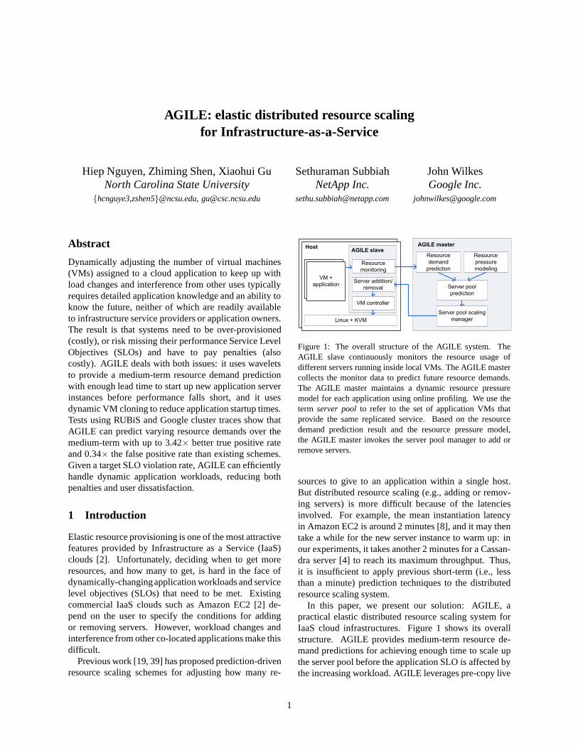
Figure 2: Wavelet decomposition of an Apache web serverCPU demand under a real web server workload from theClarkNet web server [24]. The original signal is decomposedinto four detailed signals from scale 1 to 4 and one approxi-mation signal using Haar wavelets. At each scale, the dottedline shows the predicted signal for the next future 16 secondsat time t = 32 second.

2 AGILE system design

In this section, we first describe our medium-term re-source demand prediction scheme. By “medium-term”,we mean up to 2 minutes (i.e., 60 sampling intervalsgiven a 2-second sampling interval). We then introduceour online resource pressure modeling system for map-ping SLO requirements to proper resource allocation.Next, we describe the dynamic server pool scaling mech-anism using live VM cloning.

2.1 Medium-Term Resource demand pre-diction using Wavelets

AGILE provides online resource demand predictionusing a sliding windowD (e.g., D = 6000 seconds)of recent resource usage data. AGILE does not re-quire advance application profiling or white-box/grey-box application modeling. Instead, it employswavelettransforms[1] to make its medium-term predictions: ateach sampling instantt, predicting the resource demandover the prediction window of lengthW (e.g.,W = 120

2

seconds). The basic idea is to first decompose theoriginal resource demand time series into a set of waveletbased signals. We then perform predictions for eachdecomposed signal separately. Finally, we synthesize thefuture resource demand by adding up all the individualsignal predictions. Figure 2 illustrates our wavelet-based prediction results for an Apache web server’s CPUdemand trace.

Wavelet transforms decompose a signal into a set ofwavelets at increasing scales. Wavelets at higher scaleshave larger duration, representing the original signal atcoarser granularities. Each scalei corresponds to awavelet duration ofLi seconds, typicallyLi = 2i . Forexample, in Figure 2, each wavelet at scale 1 covers 21

seconds while each wavelet at scale 4 covers 24 = 16seconds. After removing all the lower scale signalscalleddetailed signalsfrom the original signal, we obtaina smoothed version of the original signal called theapproximation signal. For example, in Figure 2, theoriginal CPU demand signal is decomposed into fourdetailed signals from scale 1 to 4, and one approximationsignal. Then the prediction of the original signal issynthesized by adding up the predictions of these decom-posed signals.

Wavelet transforms can use different basis functionssuch as the Haar and Daubechies wavelets [1]. Incontrast, Fourier transforms [6] can only use the sinusoidas the basis function, which only works well for cyclicresource demand traces. Thus, wavelet transforms haveadvantages over Fourier transforms in analyzing acyclicpatterns.

The scale signali is a series of independent non-overlapping chunks of time, each with duration of 2i

(e.g., the time intervals [0-8), [8-16)). We need to predictW/2i values to construct the scalei signal in the look-ahead windowW as adding one value will increase thelength of the scalei signal by 2i .

Since each wavelet in the higher scale signal has alarger duration, we have fewer values to predict forhigher scale signals given the same look-ahead window.Thus, it is easier to achieve accurate predictions forhigher scale signals as fewer prediction iterations areneeded. For example, in Figure 2, suppose the look-ahead window is 16 seconds, we only need to predict 1value for the approximation signal but we need to predict8 values for the scale 1 detail signal.

Wavelet transforms have two key configuration pa-rameters: 1) the wavelet function to use, and 2) thenumber of scales. AGILE dynamically configures thesetwo parameters in order to minimize the predictionerror. Since the approximation signal has fewer values topredict, we want to maximize the similarity between theapproximation signal and the original signal. For eachsliding windowD, AGILE selects the wavelet function

60 70 80 900

10

20

30

40

Resource pressure model Sample data for building the model Real data observed in experiments

Resource pressure (%)

SLO

vio

latio

n ra

te (%

)

60 70 80 900

10

20

30

40 Database tier

SLO

vio

latio

n ra

te (%

)

Resource pressure (%)

Web server tier

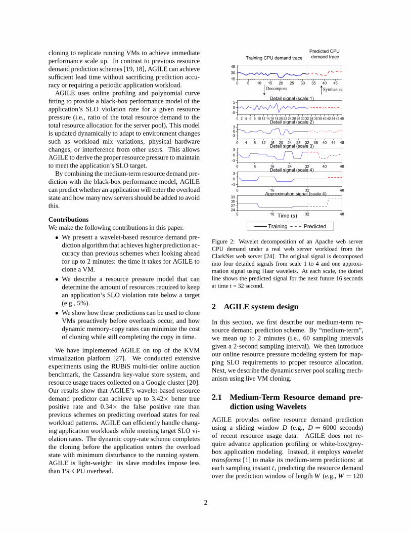
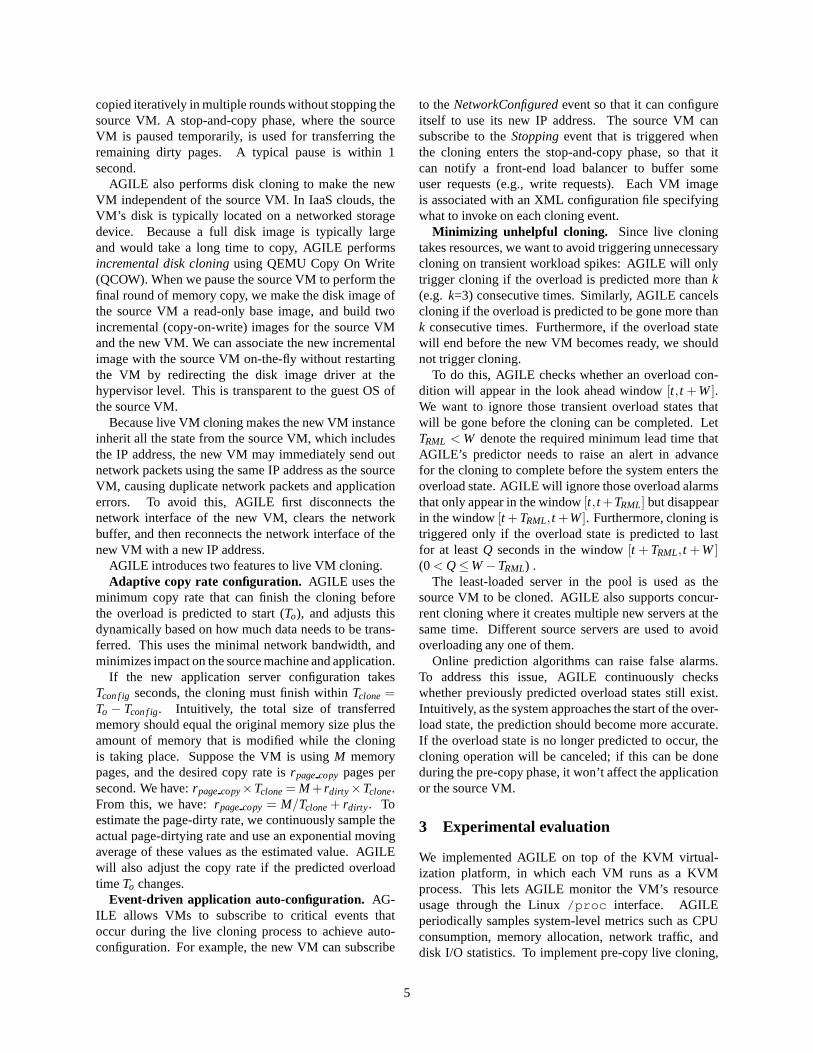
Figure 3: Dynamically derived CPU resource pressure modelsmapping from the resource pressure level to the SLO violationrate using online profiling for RUBiS web server and databaseserver. The profiling time for constructing one resource pres-sure model is about 10 to 20 minutes.

that results in the smallest Euclidean distance betweenthe approximation signal and the original signal. Then,AGILE sets the number of values to be predicted for theapproximation signal to 1. It does this by choosing thenumber of scales for the wavelet transforms. Given alook-ahead windowW, letU denote the number of scales(e.g., scale of the approximation signal). Then, we haveW/2U = 1, orU = ⌈log2(W)⌉. For example, in Figure 2,the look-ahead window is 16 seconds, so AGILE sets themaximum scale toU = ⌈log2(16)⌉= 4.

We can use different prediction algorithms for predict-ing wavelet values at different scales. In our current pro-totype, we use a simple Markov model based predictionscheme presented in [19].

2.2 Online resource pressure modeling

AGILE needs to pick an appropriate resource allocationto meet the application’s SLO. One way to do this wouldbe to predict the input workload [21] and infer the futureresource usage by constructing a model that can mapinput workload (e.g., request rate, request type mix) intothe resource requirements to meet an SLO. However,this approach often requires significant knowledge of theapplication, which is often unavailable in IaaS cloudsand might be privacy sensitive, and building an accurateworkload-to-resource demand model is nontrivial [22].

Instead, AGILE predicts an application’s resourceusage, and then uses an application-agnosticresourcepressuremodel to map the application’s SLO violationrate target (e.g.,< 5%) into a maximum resource pres-sure to maintain. Resource pressure is the ratio ofresource usage to allocation. Note that it is necessary toallocate a little more resources than predicted in order toaccommodate transient workload spikes and leave someheadroom for the application to demonstrate a need for

3

more resources [39, 33, 31]. We use online profilingto derive a resource pressure model for each applicationtier. For example, Figure 3 shows the relationship be-tween CPU resource pressure and the SLO violation ratefor the two tiers in RUBiS, and the model that AGILEfits to the data. If the user requires the SLO violation rateto be no more than 5%, the resource pressure of the webserver tier should be kept below 78% and the resourcepressure of the database tier below 77%.

The resource pressure model is application specific,and may change at runtime due to variations in theworkload mix. For example, in RUBiS, a workloadwith more write requests may require more CPU thanthe workload with more browse requests. To deal withboth issues, AGILE generates the model dynamically atruntime with an application-agnostic scheme that usesonline profiling and curve fitting.

The first step in building a new mapping functionis to collect a few pairs of resource pressure and SLOviolation rates by adjusting the application’s resourceallocation (and hence resource pressure) using the Linuxcgroups interface. If the application consists of multi-ple tiers, the profiling is performed tier by tier; when onetier is being profiled, the other tiers are allocated suffi-cient resources to make sure that they are not bottlenecks.If the application’s SLO is affected by multiple types ofresources (e.g., CPU, memory), we profile each type ofresource separately while allocating sufficient amountsof all the other resource types. We average the resourcepressures of all the servers in the profiled tier and pairthe mean resource pressure with the SLO violation ratecollected during a profiling interval (e.g., 1 minute).

AGILE fits the profiling data against a set of polyno-mials with different orders (from 2 to 16 in our experi-ment) and selects the best fitting curve using the least-square error. We set the maximum order to 16 to avoidoverfitting. At runtime, AGILE continuously monitorsthe current resource pressure and SLO violation rate, andupdates the resource pressure model with the new data. Ifthe mapping function changes significantly (e.g., due tovariations in the workload mix), and the approximationerror exceeds a pre-defined threshold (e.g., 5%), AGILEreplaces the current model with a new one. Since weneed to adjust the resource allocation gradually and waitfor the application to become stable to get a good model,it takes about 10 to 20 minutes for AGILE to derive a newresource pressure model from scratch using the onlineprofiling scheme. To avoid frequent model retraining,AGILE maintains a set of models and dynamically se-lects the best model for the current workload. Thisis useful for applications that have distinct phases ofoperation. A new model is built and added only if theapproximation errors of all current models exceed thethreshold.

0 50 100 150 2000

1000

2000

3000

Thro

ughp

ut (o

ps/s

ec)

Time (s)

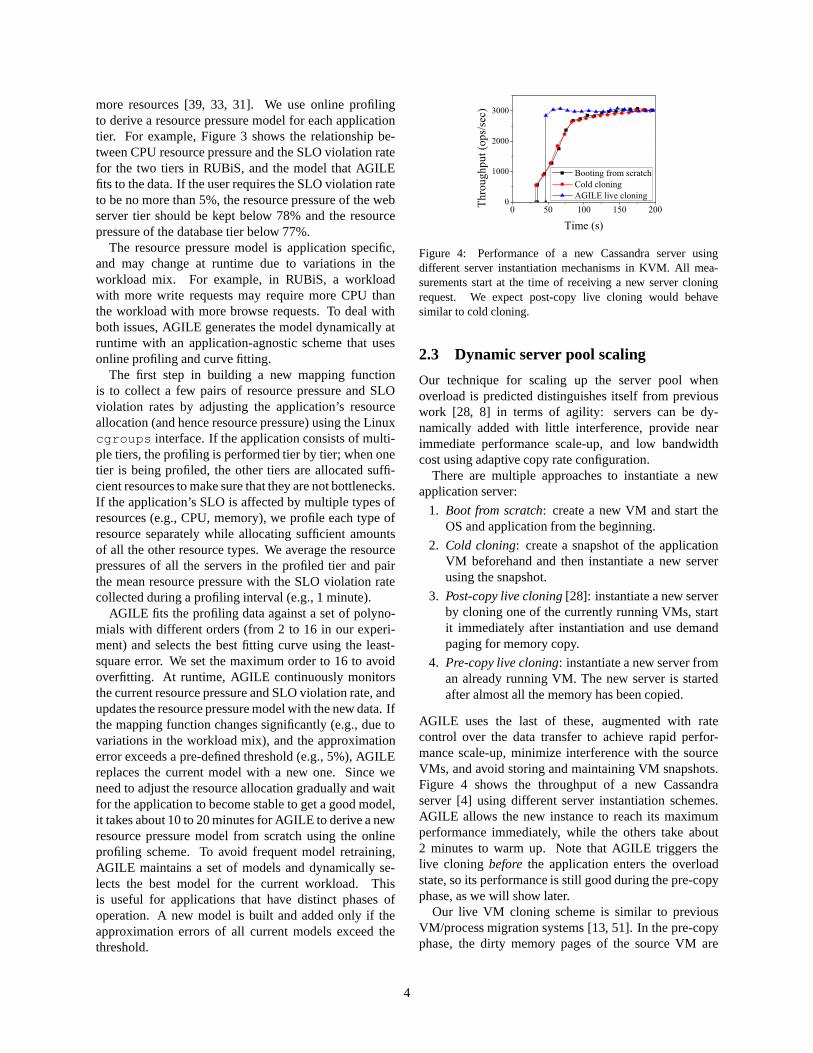
Booting from scratch Cold cloning AGILE live cloning

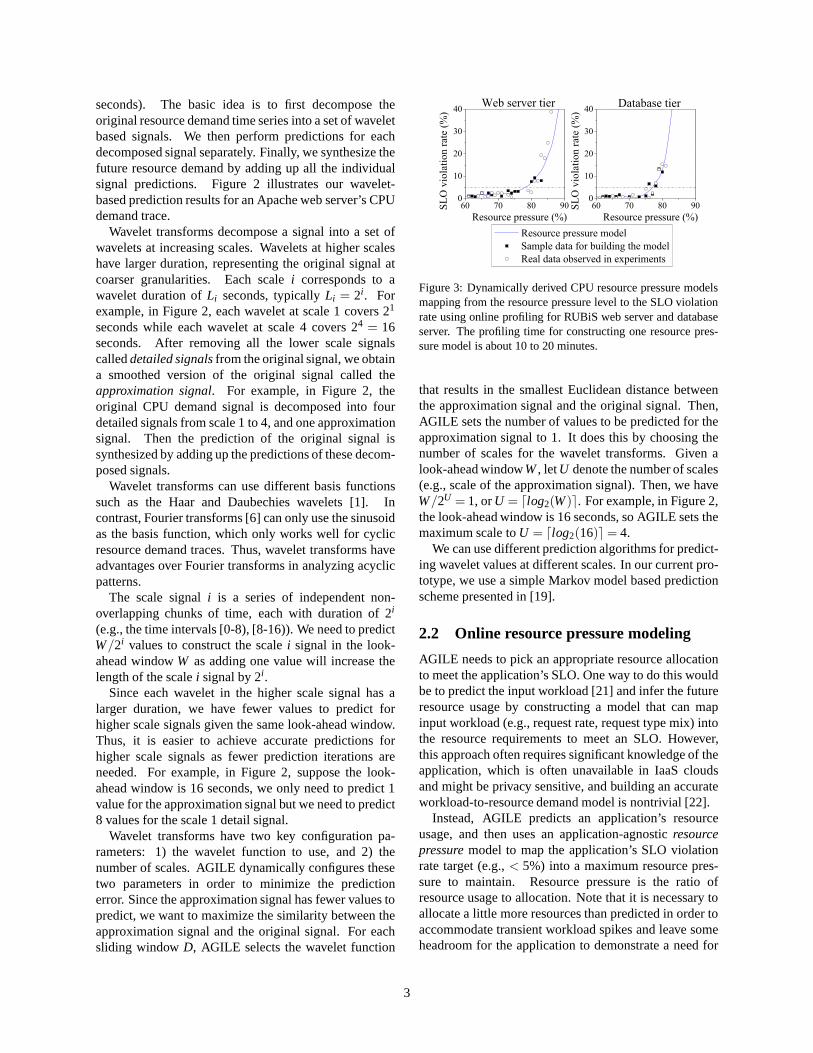
Figure 4: Performance of a new Cassandra server usingdifferent server instantiation mechanisms in KVM. All mea-surements start at the time of receiving a new server cloningrequest. We expect post-copy live cloning would behavesimilar to cold cloning.

2.3 Dynamic server pool scaling

Our technique for scaling up the server pool whenoverload is predicted distinguishes itself from previouswork [28, 8] in terms of agility: servers can be dy-namically added with little interference, provide nearimmediate performance scale-up, and low bandwidthcost using adaptive copy rate configuration.

There are multiple approaches to instantiate a newapplication server:

1. Boot from scratch: create a new VM and start theOS and application from the beginning.

2. Cold cloning: create a snapshot of the applicationVM beforehand and then instantiate a new serverusing the snapshot.

3. Post-copy live cloning[28]: instantiate a new serverby cloning one of the currently running VMs, startit immediately after instantiation and use demandpaging for memory copy.

4. Pre-copy live cloning: instantiate a new server froman already running VM. The new server is startedafter almost all the memory has been copied.

AGILE uses the last of these, augmented with ratecontrol over the data transfer to achieve rapid perfor-mance scale-up, minimize interference with the sourceVMs, and avoid storing and maintaining VM snapshots.Figure 4 shows the throughput of a new Cassandraserver [4] using different server instantiation schemes.AGILE allows the new instance to reach its maximumperformance immediately, while the others take about2 minutes to warm up. Note that AGILE triggers thelive cloning before the application enters the overloadstate, so its performance is still good during the pre-copyphase, as we will show later.

Our live VM cloning scheme is similar to previousVM/process migration systems [13, 51]. In the pre-copyphase, the dirty memory pages of the source VM are

4

copied iteratively in multiple rounds without stopping thesource VM. A stop-and-copy phase, where the sourceVM is paused temporarily, is used for transferring theremaining dirty pages. A typical pause is within 1second.

AGILE also performs disk cloning to make the newVM independent of the source VM. In IaaS clouds, theVM’s disk is typically located on a networked storagedevice. Because a full disk image is typically largeand would take a long time to copy, AGILE performsincremental disk cloningusing QEMU Copy On Write(QCOW). When we pause the source VM to perform thefinal round of memory copy, we make the disk image ofthe source VM a read-only base image, and build twoincremental (copy-on-write) images for the source VMand the new VM. We can associate the new incrementalimage with the source VM on-the-fly without restartingthe VM by redirecting the disk image driver at thehypervisor level. This is transparent to the guest OS ofthe source VM.

Because live VM cloning makes the new VM instanceinherit all the state from the source VM, which includesthe IP address, the new VM may immediately send outnetwork packets using the same IP address as the sourceVM, causing duplicate network packets and applicationerrors. To avoid this, AGILE first disconnects thenetwork interface of the new VM, clears the networkbuffer, and then reconnects the network interface of thenew VM with a new IP address.

AGILE introduces two features to live VM cloning.Adaptive copy rate configuration. AGILE uses the

minimum copy rate that can finish the cloning beforethe overload is predicted to start (To), and adjusts thisdynamically based on how much data needs to be trans-ferred. This uses the minimal network bandwidth, andminimizes impact on the source machine and application.

If the new application server configuration takesTcon f ig seconds, the cloning must finish withinTclone =To − Tcon f ig. Intuitively, the total size of transferredmemory should equal the original memory size plus theamount of memory that is modified while the cloningis taking place. Suppose the VM is usingM memorypages, and the desired copy rate isrpagecopy pages persecond. We have:rpagecopy×Tclone= M + rdirty ×Tclone.From this, we have:rpagecopy = M/Tclone+ rdirty. Toestimate the page-dirty rate, we continuously sample theactual page-dirtying rate and use an exponential movingaverage of these values as the estimated value. AGILEwill also adjust the copy rate if the predicted overloadtimeTo changes.

Event-driven application auto-configuration. AG-ILE allows VMs to subscribe to critical events thatoccur during the live cloning process to achieve auto-configuration. For example, the new VM can subscribe

to theNetworkConfiguredevent so that it can configureitself to use its new IP address. The source VM cansubscribe to theStoppingevent that is triggered whenthe cloning enters the stop-and-copy phase, so that itcan notify a front-end load balancer to buffer someuser requests (e.g., write requests). Each VM imageis associated with an XML configuration file specifyingwhat to invoke on each cloning event.

Minimizing unhelpful cloning. Since live cloningtakes resources, we want to avoid triggering unnecessarycloning on transient workload spikes: AGILE will onlytrigger cloning if the overload is predicted more thank(e.g. k=3) consecutive times. Similarly, AGILE cancelscloning if the overload is predicted to be gone more thank consecutive times. Furthermore, if the overload statewill end before the new VM becomes ready, we shouldnot trigger cloning.

To do this, AGILE checks whether an overload con-dition will appear in the look ahead window[t,t +W].We want to ignore those transient overload states thatwill be gone before the cloning can be completed. LetTRML < W denote the required minimum lead time thatAGILE’s predictor needs to raise an alert in advancefor the cloning to complete before the system enters theoverload state. AGILE will ignore those overload alarmsthat only appear in the window[t,t +TRML] but disappearin the window[t +TRML,t +W]. Furthermore, cloning istriggered only if the overload state is predicted to lastfor at leastQ seconds in the window[t + TRML,t +W](0 < Q≤W−TRML) .

The least-loaded server in the pool is used as thesource VM to be cloned. AGILE also supports concur-rent cloning where it creates multiple new servers at thesame time. Different source servers are used to avoidoverloading any one of them.

Online prediction algorithms can raise false alarms.To address this issue, AGILE continuously checkswhether previously predicted overload states still exist.Intuitively, as the system approaches the start of the over-load state, the prediction should become more accurate.If the overload state is no longer predicted to occur, thecloning operation will be canceled; if this can be doneduring the pre-copy phase, it won’t affect the applicationor the source VM.

3 Experimental evaluation

We implemented AGILE on top of the KVM virtual-ization platform, in which each VM runs as a KVMprocess. This lets AGILE monitor the VM’s resourceusage through the Linux/proc interface. AGILEperiodically samples system-level metrics such as CPUconsumption, memory allocation, network traffic, anddisk I/O statistics. To implement pre-copy live cloning,

5

we modified KVM to add a new KVM hypervisor mod-ule and an interface in theKVM monitor that supportsstarting, stopping a clone, and adjusting the memorycopy rate. AGILE controls the resources allocated toapplication VMs through the Linuxcgroups interface.

We evaluated our KVM implementation of AGILEusing the RUBiS online auction benchmark (PHP ver-sion) [38] and the Apache Cassandra key-value store0.6.13 [4]. We also tested our prediction algorithm usingGoogle cluster data [20]. This section describes ourexperiments and results.

3.1 Experiment methodology

Our experiments were conducted on a cloud testbed inour lab with 10 nodes. Each cloud node has a quad-core Xeon 2.53GHz processor, 8GiB memory and 1Gbpsnetwork bandwidth, and runs 64 bit CentOS 6.2 withKVM 0.12.1.2. Each guest VM runs 64 bit CentOS 5.2with one virtual CPU core and 2GiB memory. This setupis enough to host our test benchmarks at their maximumworkload.

Our experiments on RUBiS focus on the CPU re-source, as that appears to be the bottleneck in oursetup since all the RUBiS components have low memoryconsumption. To evaluate AGILE under workloadswith realistic time variations, we used one day of per-minute workload intensity observed in 4 different realworld web traces [24] to modulate the request rate ofthe RUBiS benchmark: (1) World Cup 98 web servertrace starting at 1998-05-05:00.00; (2) NASA web servertrace beginning at 1995-07-01:00.00; (3) EPA web servertrace starting at 1995-08-29:23.53; and (4) ClarkNet webserver trace beginning at 1995-08-28:00.00. These tracesrepresent realistic load variations over time observedfrom well-known web sites. The resource usage iscollected every 2 seconds. We perform fine-grainedsampling for precise resource usage prediction and ef-fective scaling [43]. Although the request rate is changedevery minute, the resource usage may still change fasterbecause different types of requests are generated.

At each sampling instantt, the resource demandprediction module uses a sliding window of sizeD ofrecent resource usage (i.e., fromt −D to t) and predictsfuture resource demands in the look-ahead windowW(i.e., from t to t +W). We repeat each experiment 6times.

We also tested our prediction algorithm using realsystem resource usage data collected on a Googlecluster [20] to evaluate its accuracy on predictingmachine overloads. To do this, we extracted CPUand memory usage traces from 100 machines randomlyselected from the Google cluster data. We then aggregatethe resource usages of all the tasks running on a given

Parameter RUBiS Google dataInput data window (D) 6000 seconds 250 hoursLook-ahead window (W) 120 seconds 5 hoursSampling interval (Ts) 2 seconds 5 minutesTotal trace length one day 29 daysOverload duration threshold (Q) 20 seconds 25 minutesResponse time SLO 100 ms NA

Table 1: Summary of parameter values used in our experiments.

machine to get the usage for that machine. Thesetraces represent various realistic workload patterns. Thesampling interval in the Google cluster is 5 minutes andthe trace lasts 29 days.

Table 1 shows the parameter values used in ourexperiments. We also performed comparisons underdifferent threshold values by varyingD,W, andQ, whichshow similar trends. Note that we used consistentlylarger D, W, and Q values for the Google trace databecause the sampling interval of the Google data (5minutes) is significantly larger than what we used in theRUBiS experiments (2 seconds).

To evaluate the accuracy of our wavelet-basedprediction scheme, we compare it against the bestalternatives we could find: PRESS [19] and auto-regression [9]. These have been shown to achievehigher accuracy and lower overheads than otheralternatives. We calculate the overload-predictionaccuracy as follows. The predictor is deemed toraise a valid overload alarm if the overload state(e.g., when the resource pressure is bigger than theoverload threshold) is predicted earlier than the requiredminimum lead time (TRML). Otherwise, we call theprediction a false negative. Note that we only considerthose overload states that last at leastQ seconds(Section 2.3). Moreover, we require that the predictionmodel accurately estimates when the overload will start,so we compare the predicted alarm time with the trueoverload start time to calculate aprediction time error. Ifthe absolute prediction time error is small (i.e.,≤ 3 ·Ts),we say the predictor raises a correct alarm. Otherwise,we say the predictor raises a false alarm.

We use the standard metrics,true positive rate(AT)and false positive rate(AF ), given in equation 1.Ptrue, Pfalse, Ntrue, and Nfalse denote the number oftrue positives, false positives, true negatives, and falsenegatives, respectively.

AT =Ptrue

Ptrue+Nf alse, AF =

Pf alse

Pf alse+Ntrue(1)

A service provider can either rely on the applicationitself or an external tool [5] to tell whether the applicationSLO is being violated. In our experiments, we adoptedthe latter approach. With the RUBiS benchmark, the

6

WorldCup NASA EPA ClarkNet0

25

50

75

100

True

pos

itive

rate

(%)

Wavelet-60 Wavelet-100 PRESS-60 PRESS-100 AutoRegression-60 AutoRegression-100

(a)

WorldCup NASA EPA ClarkNet0

10

20

30

40

50

Fals

e po

sitiv

e ra

te (%

)

Wavelet-60 Wavelet-100 PRESS-60 PRESS-100 AutoRegression-60 AutoRegression-100

(b)

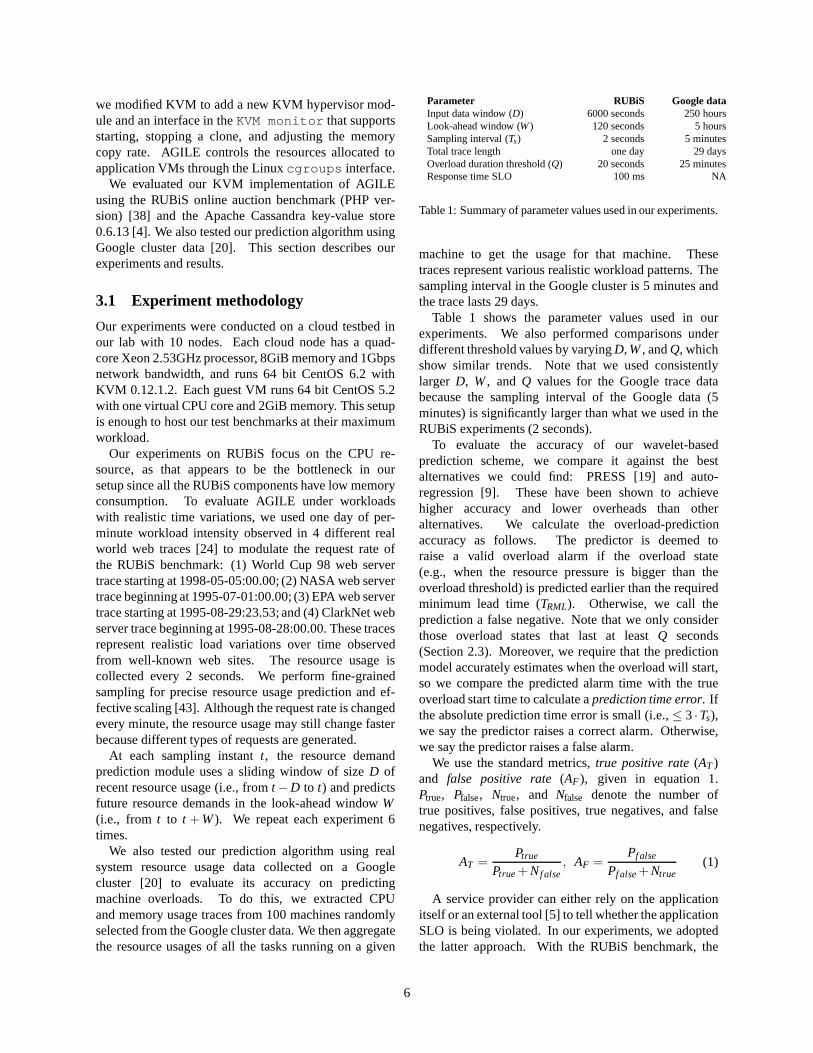
Figure 5: CPU demand prediction accuracy comparison forRUBiS web server driven by one-day request traces of differentreal web servers withTRML = 60 and 100 seconds.

workload generator tracks the response time of the HTTPrequests it makes. The SLO violation rate is the fractionof requests that have response time larger than a pre-defined SLO threshold. In our experiments, this was100ms, the 99th percentile of observed response timesfor a run with no resource constraints. We conduct ourRUBiS experiments on both the Apache web server tierand the MySQL database tier.

For comparison, we also implemented a set ofalternative resource provisioning schemes:

• No scaling: A non-elastic resource provisioningscheme that cannot change the size of the serverpool, which is fixed at 1 server as this is sufficientfor the average resource demand.

• Reactive: This scheme triggers live VM cloningwhen it observes that the application has becomeoverloaded. It uses a fixed memory-copy rate, andfor a fair comparison, we set this to the average copyrate used by AGILE so that both schemes incur asimilar network cost for cloning.

• PRESS: Instead of using the wavelet-basedprediction algorithm, PRESS uses a Markov+FFTresource demand prediction algorithm [19] topredict future overload state and triggers livecloning when an overload state is predicted tooccur. PRESS uses the same false alarm filtering

1 10 100 10000

20

40

60

80

100

Wavelet-60 PRESS-60 AutoRegression-60

Absolute prediction time error (s) [log10

]Cum

ulat

ive

dist

ribut

ion

func

tion

(%)

0

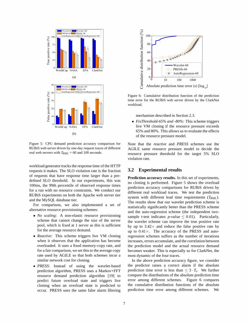
Figure 6: Cumulative distribution function of the predictiontime error for the RUBiS web server driven by the ClarkNetworkload.

mechanism described in Section 2.3.

• FixThreshold-65% and -80%: This scheme triggerslive VM cloning if the resource pressure exceeds65% and 80%. This allows us to evaluate the effectsof the resource pressure model.

Note that thereactive and PRESSschemes use theAGILE same resource pressure model to decide theresource pressure threshold for the target 5% SLOviolation rate.

3.2 Experimental results

Prediction accuracy results.In this set of experiments,no cloning is performed. Figure 5 shows the overloadprediction accuracy comparisons for RUBiS driven bydifferent real workload traces. We test the predictionsystem with different lead time requirements (TRML).The results show that our wavelet prediction scheme isstatistically significantly better than the PRESS schemeand the auto-regression scheme (the independent two-sample t-test indicatesp-value≤ 0.01). Particularly,the wavelet scheme can improve the true positive rateby up to 3.42× and reduce the false positive rate byup to 0.41×. The accuracy of the PRESS and auto-regression schemes suffers as the number of iterationsincreases, errors accumulate, and the correlation betweenthe prediction model and the actual resource demandbecomes weaker. This is especially so for ClarkNet, themost dynamic of the four traces.

In the above prediction accuracy figure, we considerthe predictor raises a correct alarm if the absoluteprediction time error is less than≤ 3 · Ts. We furthercompare the distributions of the absolute prediction timeerror among different schemes. Figure 6 comparesthe cumulative distribution functions of the absoluteprediction time error among different schemes. We

7

Wavelet-100

Wavelet-150

PRESS-100

PRESS-150

AutoRegression-100

AutoRegression-150

0

20

40

60

80

100

True

pos

itive

rate

(%)

(a)

Wavelet-100

Wavelet-150

PRESS-100

PRESS-150

AutoRegression-100

AutoRegression-150

0

20

40

60

Fals

e po

sitiv

e ra

te (%

)

(b)

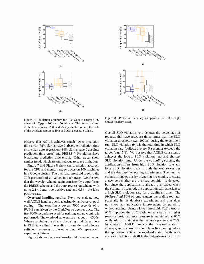
Figure 7: Prediction accuracy for 100 Google cluster CPUtraces withTRML = 100 and 150 minutes. The bottom and topof the box represent 25th and 75th percentile values, the endsof the whiskers represent 10th and 90th percentile values.

observe that AGILE achieves much lower predictiontime error (78% alarms have 0 absolute prediction timeerror) than auto-regression (34% alarms have 0 absoluteprediction time error) and PRESS (46% alarms have0 absolute prediction time error). Other traces showsimilar trend, which are omitted due to space limitation.

Figure 7 and Figure 8 show the prediction accuracyfor the CPU and memory usage traces on 100 machinesin a Google cluster. The overload threshold is set to the70th percentile of all values in each trace. We observethat the wavelet scheme again consistently outperformsthe PRESS scheme and the auto-regression scheme withup to 2.1× better true positive rate and 0.34× the falsepositive rate.

Overload handling results. Next, we evaluate howwell AGILE handles overload using dynamic server poolscaling. The experiment covers 7000 seconds of aRUBiS run driven by the ClarkNet web server trace. Thefirst 6000 seconds are used for training and no cloning isperformed. The overload state starts at about t = 6500s.When examining the effects of scaling on different tiersin RUBiS, we limit the scaling to one tier and allocatesufficient resources to the other tier. We repeat eachexperiment 3 times.

Figure 9 shows the overall results of different schemes.

Wavelet-100

Wavelet-150

PRESS-100

PRESS-150

AutoRegression-100

AutoRegression-150

0

20

40

60

80

100

True

pos

itive

rate

(%)

(a)

Wavelet-100

Wavelet-150

PRESS-100

PRESS-150

AutoRegression-100

AutoRegression-150

0

20

40

60

80

Fals

e po

sitiv

e ra

te (%

)

(b)

Figure 8: Prediction accuracy comparison for 100 Googlecluster memory traces.

Overall SLO violationrate denotes the percentage ofrequests that have response times larger than the SLOviolation threshold (e.g., 100ms) during the experimentrun. SLO violationtime is the total time in which SLOviolation rate (collected every 5 seconds) exceeds thetarget (e.g., 5%). We observe that AGILE consistentlyachieves the lowest SLO violation rate and shortestSLO violation time. Under theno scalingscheme, theapplication suffers from high SLO violation rate andlong SLO violation time in both the web server tierand the database tier scaling experiments. Thereactivescheme mitigates this by triggering live cloning to createa new server after the overload condition is detected,but since the application is already overloaded whenthe scaling is triggered, the application still experiencesa high SLO violation rate for a significant time. TheFixThreshold-80%scheme triggers the scaling too late,especially in the database experiment and thus doesnot show any noticeable improvement compared towithout scaling. Using a lower threshold,FixThreshold-65% improves the SLO violation rate but at a higherresource cost: resource pressure is maintained at 65%while AGILE maintains the resource pressure at 75%.In contrast, AGILE predicts the overload state inadvance, and successfully completes live cloning beforethe application enters the overload state. With moreaccurate predictions, AGILE also outperforms PRESS by

8

0

5

10

15

20O

vera

ll SL

O v

iola

tion

rate

(%)

No scaling Reactive PRESS AGILE FixThreshold-65% FixThreshold-80%

0

50

100

150

200 4024185035302727.2

Ove

rall

SLO

vio

latio

n tim

e (s

)

DatabaseWebserver

DatabaseWebserver

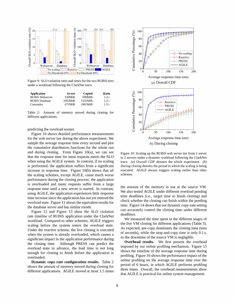
Figure 9: SLO violation rates and times for the two RUBiS tiersunder a workload following the ClarkNet trace.

Application In use Copied RatioRUBiS Webserver 530MiB 690MiB 1.3×RUBiS Database 1092MiB 1331MiB 1.2×Cassandra 671MiB 1001MiB 1.5×

Table 2: Amount of memory moved during cloning fordifferent applications.

predicting the overload sooner.Figure 10 shows detailed performance measurements

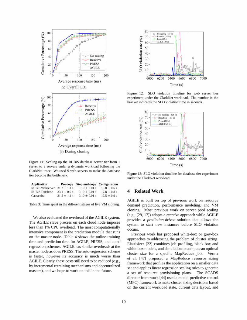
for the web server tier during the above experiment. Wesample the average response time every second and plotthe cumulative distribution functions for the whole runand during cloning. From Figure 10(a), we can seethat the response time for most requests meets the SLOwhen using the AGILE system. In contrast, if no scalingis performed, the application suffers from a significantincrease in response time. Figure 10(b) shows that allthe scaling schemes, except AGILE, cause much worseperformance during the cloning process: the applicationis overloaded and many requests suffer from a largeresponse time until a new server is started. In contrast,using AGILE, the application experiences little responsetime increase since the application has not yet entered theoverload state. Figure 11 shows the equivalent results forthe database server and has similar trends.

Figure 12 and Figure 13 show the SLO violationrate timeline of RUBiS application under the ClarkNetworkload. Compared to other schemes, AGILE triggersscaling before the system enters the overload state.Under the reactive scheme, the live cloning is executedwhen the system is already overloaded, which causes asignificant impact to the application performance duringthe cloning time. Although PRESS can predict theoverload state in advance, the lead time is not longenough for cloning to finish before the application isoverloaded.

Dynamic copy-rate configuration results. Table 2shows the amount of memory moved during cloning fordifferent applications. AGILE moved at most 1.5 times

0 50 100 150 2000

20

40

60

80

100

No scaling Reactive PRESS AGILE

Average response time (ms)

Cum

ulat

ive

Perc

enta

ge (%

)

(a) Overall CDF

0 50 100 150 2000

20

40

60

80

100

Reactive PRESS AGILE

Average response time (ms)Cu

mul

ativ

e Pe

rcen

tage

(%)

(b) During cloning

Figure 10: Scaling up the RUBiS web server tier from 1 serverto 2 servers under a dynamic workload following the ClarkNettrace. (a) Overall CDF denotes the whole experiment.(b)During cloningdenotes the period in which the scaling is beingexecuted. AGILE always triggers scaling earlier than otherschemes.

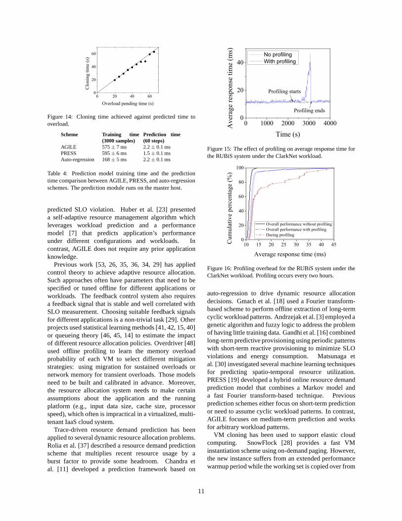
the amount of the memory in use at the source VM.We also tested AGILE under different overload pendingtime deadlines (i.e., target time to finish cloning) andcheck whether the cloning can finish within the pendingtime. Figure 14 shows that our dynamic copy-rate settingcan accurately control the cloning time under differentdeadlines.

We measured the time spent in the different stages ofthe live VM cloning for different applications (Table 3).As expected, pre-copy dominates the cloning time (tensof seconds), while the stop-and-copy time is only 0.1 s,so the downtime of the source VM is negligible.

Overhead results. We first present the overheadimposed by our online profiling mechanism. Figure 15shows the timeline of the average response time duringprofiling. Figure 16 shows the performance impact of theonline profiling on the average response time over theperiod of 6 hours, in which AGILE performs profilingthree times. Overall, the overhead measurements showthat AGILE is practical for online system management.

9

0 50 100 150 2000

20

40

60

80

100

No scaling Reactive PRESS AGILE

Average response time (ms)

Cum

ulat

ive

Perc

enta

ge (%

)

(a) Overall CDF

0 50 100 150 2000

20

40

60

80

100

Reactive PRESS AGILE

Average response time (ms)

Cum

ulat

ive

Perc

enta

ge (%

)

(b) During cloning

Figure 11: Scaling up the RUBiS database server tier from 1server to 2 servers under a dynamic workload following theClarkNet trace. We used 9 web servers to make the databasetier become the bottleneck.

Application Pre-copy Stop-and-copy ConfigurationRUBiS Webserver 31.2± 1.1 s 0.10± 0.01 s 16.8± 0.6 sRUBiS Database 33.1± 0.9 s 0.10± 0.01 s 17.8± 0.8 sCassandra 31.5± 1.1 s 0.10± 0.01 s 17.5± 0.9 s

Table 3: Time spent in the different stages of live VM cloning.

We also evaluated the overhead of the AGILE system.The AGILE slave process on each cloud node imposesless than 1% CPU overhead. The most computationallyintensive component is the prediction module that runson the master node. Table 4 shows the online trainingtime and prediction time for AGILE, PRESS, and auto-regression schemes. AGILE has similar overheads at themaster node as does PRESS. The auto-regression schemeis faster, however its accuracy is much worse thanAGILE. Clearly, these costs still need to be reduced (e.g.,by incremental retraining mechanisms and decentralizedmasters), and we hope to work on this in the future.

6000 6200 6400 6600 6800 70000

1020304050607080

No scaling (455 s) Reactive (120 s) Press (85 s) AGILE (40 s)

Time (s)

SLO

vio

latio

n ra

te (%

)

Figure 12: SLO violation timeline for web server tierexperiment under the ClarkNet workload. The number in thebracket indicates the SLO violation time in seconds.

6000 6200 6400 6600 6800 700001020304050607080

No scaling (425 s) Reactive (110 s) Press (80 s) AGILE (25 s)

Time (s)

SLO

vio

latio

n ra

te (%

)

Figure 13: SLO violation timeline for database tier experimentunder the ClarkNet workload.

4 Related Work

AGILE is built on top of previous work on resourcedemand prediction, performance modeling, and VMcloning. Most previous work on server pool scaling(e.g., [29, 17]) adopts areactiveapproach while AGILEprovides aprediction-drivensolution that allows thesystem to start new instances before SLO violationoccurs.

Previous work has proposed white-box or grey-boxapproaches to addressing the problem of cluster sizing.Elastisizer [22] combines job profiling, black-box andwhite-box models, and simulation to compute an optimalcluster size for a specific MapReduce job. Vermaet al. [47] proposed a MapReduce resource sizingframework that profiles the application on a smaller dataset and applies linear regression scaling rules to generatea set of resource provisioning plans. The SCADSdirector framework [44] used a model-predictive control(MPC) framework to make cluster sizing decisions basedon the current workload state, current data layout, and

10

0 20 40 600

20

40

60

Clo

ning

tim

e (s

)

Overload pending time (s)

Figure 14: Cloning time achieved against predicted time tooverload.

Scheme Training time(3000 samples)

Prediction time(60 steps)

AGILE 575± 7 ms 2.2± 0.1 msPRESS 595± 6 ms 1.5± 0.1 msAuto-regression 168± 5 ms 2.2± 0.1 ms

Table 4: Prediction model training time and the predictiontime comparison between AGILE, PRESS, and auto-regressionschemes. The prediction module runs on the master host.

predicted SLO violation. Huber et al. [23] presenteda self-adaptive resource management algorithm whichleverages workload prediction and a performancemodel [7] that predicts application’s performanceunder different configurations and workloads. Incontrast, AGILE does not require any prior applicationknowledge.

Previous work [53, 26, 35, 36, 34, 29] has appliedcontrol theory to achieve adaptive resource allocation.Such approaches often have parameters that need to bespecified or tuned offline for different applications orworkloads. The feedback control system also requiresa feedback signal that is stable and well correlated withSLO measurement. Choosing suitable feedback signalsfor different applications is a non-trivial task [29]. Otherprojects used statistical learning methods [41, 42, 15, 40]or queueing theory [46, 45, 14] to estimate the impactof different resource allocation policies. Overdriver [48]used offline profiling to learn the memory overloadprobability of each VM to select different mitigationstrategies: using migration for sustained overloads ornetwork memory for transient overloads. Those modelsneed to be built and calibrated in advance. Moreover,the resource allocation system needs to make certainassumptions about the application and the runningplatform (e.g., input data size, cache size, processorspeed), which often is impractical in a virtualized, multi-tenant IaaS cloud system.

Trace-driven resource demand prediction has beenapplied to several dynamic resource allocation problems.Rolia et al. [37] described a resource demand predictionscheme that multiplies recent resource usage by aburst factor to provide some headroom. Chandra etal. [11] developed a prediction framework based on

0 1000 2000 3000 40000

20

40

Profiling starts

No profiling With profiling

Time (s)

Ave

rage

resp

onse

tim

e (m

s)

Profiling ends

Figure 15: The effect of profiling on average response time forthe RUBiS system under the ClarkNet workload.

10 15 20 25 30 35 40 450

20

40

60

80

100

Overall performance without profiling Overall performance with profiling During profiling

Average response time (ms)

Cum

ulat

ive

perc

enta

ge (%

)

Figure 16: Profiling overhead for the RUBiS system under theClarkNet workload. Profiling occurs every two hours.

auto-regression to drive dynamic resource allocationdecisions. Gmach et al. [18] used a Fourier transform-based scheme to perform offline extraction of long-termcyclic workload patterns. Andrzejak et al. [3] employed agenetic algorithm and fuzzy logic to address the problemof having little training data. Gandhi et al. [16] combinedlong-term predictive provisioning using periodic patternswith short-term reactive provisioning to minimize SLOviolations and energy consumption. Matsunaga etal. [30] investigated several machine learning techniquesfor predicting spatio-temporal resource utilization.PRESS [19] developed a hybrid online resource demandprediction model that combines a Markov model anda fast Fourier transform-based technique. Previousprediction schemes either focus on short-term predictionor need to assume cyclic workload patterns. In contrast,AGILE focuses on medium-term prediction and worksfor arbitrary workload patterns.

VM cloning has been used to support elastic cloudcomputing. SnowFlock [28] provides a fast VMinstantiation scheme using on-demand paging. However,the new instance suffers from an extended performancewarmup period while the working set is copied over from

11

the origin. Kaleidoscope [8] uses fractional VM cloningwith VM state coloring to prefetch semantically-relatedregions. Although our current prototype uses full pre-copy, AGILE could readily work with fractional pre-copy too: prediction-driven live cloning and dynamiccopy rate adjustment can be applied to both cases.Fractional pre-copy could be especially useful if theoverload duration is predicted to be short. Dolly [10]proposed a proactive database provisioning scheme thatcreates a new database instance in advance from a diskimage snapshot and replays the transaction log to bringthe new instance to the latest state. However, Dolly didnot provide any performance predictions, and the newinstance created from an image snapshot may need somewarmup time. In contrast, the new instance created byAGILE can reach its peak performance immediately afterstart.

Local resource scaling (e.g., [39]) or live VMmigration [13, 50, 49, 25] can also relieve local, per-server application overloads, but distributed resourcescaling will be needed if the workload exceeds themaximum capacity of any single server. Althoughprevious work [39, 50] has used overload predictionto proactively trigger local resource scaling or liveVM migration, AGILE addresses the specific challengesof using predictions in distributed resource scaling.Compared to local resource scaling and migration,cloning requires longer lead time and is more sensitiveto prediction accuracy, since we need to pay the costof maintaining extra servers. AGILE provides medium-term predictions to tackle this challenge.

5 Future Work

Although AGILE showed its practicality and efficiencyin experiments, there are several limitations which weplan to address in our future work.

AGILE currently derives resource pressure modelsfor just CPU. Our future work will extend the resourcepressure model to consider other resources such asmemory, network bandwidth, and disk I/O. There aretwo ways to build a multi-resource model. We can buildone resource pressure model for each resource separatelyor build a single resource pressure model incorporatingall of them. We plan to explore both approaches andcompare them.

AGILE currently uses resource capping (a Linuxcgroups feature) to achieve performance isolationamong different VMs [39]. Although we observed thatthe resource capping scheme works well for commonbottleneck resources such as CPU and memory, theremay still exist interference among co-located VMs [52].We need to take such interference into account to buildmore precise resource pressure models and achieve more

accurate overload predictions.Our resource pressure model profiling can be triggered

either periodically or by workload mix changes. Tomake AGILE more intelligent, we plan to incorporateworkload change detection mechanism [32, 12] inAGILE. Upon detecting a workload change, AGILEstarts a new profiling phase to build a new resourcepressure model for the current workload type.

6 Conclusion

AGILE is an application-agnostic, prediction-driven,distributed resource scaling system for IaaS clouds.It uses wavelets to provide medium-term performancepredictions; it provides an automatically-determinedmodel of how an application’s performance relates tothe resources it has available; and it implements a wayof cloning VMs that minimizes application startup time.Together, these allow AGILE to predict performanceproblems far enough in advance that they can be avoided.

To minimize the impact of cloning a VM, AGILEcopies memory at a rate that completes the clone justbefore the new VM is needed. AGILE performscontinuous prediction validation to detect false alarmsand cancels unnecessary cloning.

We implemented AGILE on top of the KVMvirtualization platform, and conducted experimentsunder a number of time-varying application loadsderived from real-life web workload traces and realresource usage traces. Our results show that AGILE cansignificantly reduce SLO violations when compared toexisting resource scaling schemes. Finally, AGILE islightweight, which makes it practical for IaaS clouds.

7 Acknowledgement

This work was sponsored in part by NSF CNS0915567grant, NSF CNS0915861 grant, NSF CAREER AwardCNS1149445, U.S. Army Research Office (ARO) undergrant W911NF-10-1-0273, IBM Faculty Awards andGoogle Research Awards. Any opinions expressed inthis paper are those of the authors and do not necessarilyreflect the views of NSF, ARO, or U.S. Government.

References

[1] N. A. Ali and R. H. Paul.Multiresolution signaldecomposition. Academic Press, 2000.

[2] Amazon Elastic Compute Cloud.http://aws.amazon.com/ec2/.

[3] A. Andrzejak, S. Graupner, and S. Plantikow. Predictingresource demand in dynamic utility computingenvironments. InAutonomic and Autonomous Systems,2006.

12

[4] Apache Cassandra Database.http://cassandra.apache.org/.

[5] M. Ben-Yehuda, D. Breitgand, M. Factor, H. Kolodner,V. Kravtsov, and D. Pelleg. NAP: a building block forremediating performance bottlenecks via black boxnetwork analysis. InICAC, 2009.

[6] E. Brigham and R. Morrow. The fast Fourier transform.IEEE Spectrum, 1967.

[7] F. Brosig, N. Huber, and S. Kounev. Automatedextraction of architecture-level performance models ofdistributed component-based systems. InAutomatedSoftware Engineering, 2011.

[8] R. Bryant, A. Tumanov, O. Irzak, A. Scannell, K. Joshi,M. Hiltunen, A. Lagar-Cavilla, and E. de Lara.Kaleidoscope: cloud micro-elasticity via VM statecoloring. InEuroSys, 2011.

[9] E. S. Buneci and D. A. Reed. Analysis of applicationheartbeats: Learning structural and temporal features intime series data for identification of performanceproblems. InSupercomputing, 2008.

[10] E. Cecchet, R. Singh, U. Sharma, and P. Shenoy. Dolly:virtualization-driven database provisioning for the cloud.In VEE, 2011.

[11] A. Chandra, W. Gong, and P. Shenoy. Dynamic resourceallocation for shared data centers using onlinemeasurements. InIWQoS, 2003.

[12] L. Cherkasova, K. Ozonat, N. Mi, J. Symons, andE. Smirni. Anomaly? application change? or workloadchange? towards automated detection of applicationperformance anomaly and change. InDependableSystems and Networks, 2008.

[13] C. Clark, K. Fraser, S. Hand, J. G. Hansen, E. Jul,C. Limpach, I. Pratt, and A. Warfield. Live migration ofvirtual machines. InNSDI, 2005.

[14] R. P. Doyle, J. S. Chase, O. M. Asad, W. Jin, and A. M.Vahdat. Model-based resource provisioning in a webservice utility. InUSENIX Symposium on InternetTechnologies and Systems, 2003.

[15] A. Ganapathi, H. Kuno, U. Dayal, J. L. Wiener, A. Fox,M. Jordan, and D. Patterson. Predicting multiple metricsfor queries: better decisions enabled by machinelearning. InInternational Conference on DataEngineering, 2009.

[16] A. Gandhi, Y. Chen, D. Gmach, M. Arlitt, andM. Marwah. Minimizing data center sla violations andpower consumption via hybrid resource provisioning. InGreen Computing Conference and Workshops, 2011.

[17] A. Gandhi, M. Harchol-Balter, R. Raghunathan, andM. Kozuch. Autoscale: Dynamic, robust capacitymanagement for multi-tier data centers. InTransactionson Computer Systems, 2012.

[18] D. Gmach, J. Rolia, L. Cherkasova, and A. Kemper.Capacity management and demand prediction for nextgeneration data centers. InInternational Conference onWeb Services, 2007.

[19] Z. Gong, X. Gu, and J. Wilkes. PRESS: PRedictiveElastic ReSource Scaling for cloud systems. InInternational Conference on Network and ServiceManagement, 2010.

[20] Google cluster-usage traces: format + scheme(2011.11.08 external).http://goo.gl/5uJri.

[21] N. R. Herbst, N. Huber, S. Kounev, and E. Amrehn.Self-adaptive workload classification and forecasting forproactive resource provisioning. InInternationalConference on Performance Engineering, 2013.

[22] H. Herodotou, F. Dong, and S. Babu. No one (cluster)size fits all: automatic cluster sizing for data-intensiveanalytics. InSoCC, 2011.

[23] N. Huber, F. Brosig, and S. Kounev. Model-basedself-adaptive resource allocation in virtualizedenvironments. InSoftware Engineering for Adaptive andSelf-Managing Systems, 2011.

[24] The IRCache Project.http://www.ircache.net/.

[25] C. Isci, J. Liu, B. Abali, J. Kephart, and J. Kouloheris.Improving server utilization using fast virtual machinemigration. InIBM Journal of Research andDevelopment, 2011.

[26] E. Kalyvianaki, T. Charalambous, and S. Hand.Self-adaptive and self-configured CPU resourceprovisioning for virtualized servers using Kalman filters.In ICAC, 2009.

[27] A. Kivity, Y. Kamay, D. Laor, U. Lublin, and A. Liguori.kvm: the linux virtual machine monitor. InLinuxSymposium, 2007.

[28] H. A. Lagar-Cavilla, J. A. Whitney, A. M. Scannell,P. Patchin, S. M. Rumble, E. de Lara, M. Brudno, andM. Satyanarayanan. SnowFlock: rapid virtual machinecloning for cloud computing. InEuroSys, 2009.

[29] H. C. Lim, S. Babu, and J. S. Chase. Automated controlfor elastic storage. InICAC, 2010.

[30] A. Matsunaga and J. Fortes. On the use of machinelearning to predict the time and resources consumed byapplications. InCluster, Cloud and Grid Computing,2010.

[31] A. Neogi, V. R. Somisetty, and C. Nero. Optimizing thecloud infrastructure: tool design and a case study.International IBM Cloud Academy Conference, 2012.

[32] H. Nguyen, Z. Shen, Y. Tan, and X. Gu. FChain: Towardblack-box online fault localization for cloud systems. InICDCS, 2013.

[33] Oracle. Best practices for database consolidation inprivate clouds, 2012.http://www.oracle.com/technetwork/database/focus-areas/database-cloud/database-cons-best-practices-1561461.pdf.

[34] P. Padala, K.-Y. Hou, K. G. Shin, X. Zhu, M. Uysal,Z. Wang, S. Singhal, and A. Merchant. Automated

13

control of multiple virtualized resources. InEuroSys,2009.

[35] P. Padala, K. G. Shin, X. Zhu, M. Uysal, Z. Wang,S. Singhal, A. Merchant, and K. Salem. Adaptive controlof virtualized resources in utility computingenvironments. InEuroSys, 2007.

[36] S. Parekh, N. Gandhi, J. Hellerstein, D. Tilbury,T. Jayram, and J. Bigus. Using control theory to achieveservice level objectives in performance management. InReal-Time Systems, 2002.

[37] J. Rolia, L. Cherkasova, M. Arlitt, and V. Machiraju.Supporting application quality of service in sharedresource pools.Communications of the ACM, 2006.

[38] RUBiS Online Auction System.http://rubis.ow2.org/.

[39] Z. Shen, S. Subbiah, X. Gu, and J. Wilkes. CloudScale:elastic resource scaling for multi-tenant cloud systems.In SoCC, 2011.

[40] P. Shivam, S. Babu, and J. Chase. Active and acceleratedlearning of cost models for optimizing scientificapplications. InVLDB, 2006.

[41] P. Shivam, S. Babu, and J. S. Chase. Learningapplication models for utility resource planning. InICAC, 2006.

[42] C. Stewart, T. Kelly, A. Zhang, and K. Shen. A dollarfrom 15 cents: cross-platform management for internetservices. InUSENIX ATC, 2008.

[43] Y. Tan, V. Venkatesh, and X. Gu. Resilientself-compressive monitoring for large-scale hostinginfrastructures. InTPDS, 2012.

[44] B. Trushkowsky, P. Bodı́k, A. Fox, M. J. Franklin, M. I.Jordan, and D. A. Patterson. The SCADS director:scaling a distributed storage system under stringentperformance requirements. InFAST, 2011.

[45] B. Urgaonkar and A. Chandra. Dynamic provisioning ofmulti-tier internet applications. InICAC, 2005.

[46] B. Urgaonkar, G. Pacifici, P. Shenoy, M. Spreitzer, andA. Tantawi. An analytical model for multi-tier internetservices and its applications. InSIGMETRICS, 2005.

[47] A. Verma, L. Cherkasova, and R. Campbell. Resourceprovisioning framework for MapReduce jobs withperformance goals. InMiddleware, 2011.

[48] D. Williams, H. Jamjoom, Y. Liu, and H. Weatherspoon.Overdriver: Handling memory overload in anoversubscribed cloud. InVEE, 2011.

[49] D. Williams, H. Jamjoom, and H. Weatherspoon. TheXen-Blanket: virtualize once, run everywhere. InEurosys, 2012.

[50] T. Wood, P. J. Shenoy, A. Venkataramani, and M. S.Yousif. Black-box and gray-box strategies for virtualmachine migration. InNSDI, 2007.

[51] E. Zayas. Attacking the process migration bottleneck.InSOSP, 1987.

[52] X. Zhang, E. Tune, R. Hagmann, R. J. V. Gokhale, andJ. Wilkes. Cpi2: Cpu performance isolation for sharedcompute clusters. InEurosys, 2013.

[53] X. Zhu, D. Young, B. J. Watson, Z. Wang, J. Rolia,S. Singhal, B. McKee, C. Hyser, D. Gmach, R. Gardner,T. Christian, and L. Cherkasova. 1000 Islands:integrated capacity and workload management for thenext generation data center. InICAC, 2008.

14