Elasticity of Demand and SupplyChapter 4

LIPSEY & CHRYSTAL

ECONOMICS 12e

Introduction

• The demand and supply analysis helps us to understand the direction in which price and quantity would change in response to shifts in demand or supply.

• What economists would like to know is ‘what will happen to demand/supply when price changes?’

Learning Outcomes

• Here we extend our understanding of supply and demand and consider the following:

• How the sensitivity of quantity demanded to a change in price is measured by the elasticity of demand and what factors influence it.

• How elasticity is measured at a point or over a range.• How income elasticity is measured and how it varies with

different types of goods.• How elasticity of supply is measured and what it tells us

about conditions of production.• Some of the difficulties that arise in trying to estimate

various elasticities from sales data.

Price elasticity of demand

• Demand elasticity is measured by a ratio: the percentage change in quantity demanded divided by the percentage change in price that brought it about.

• For normal, negatively sloped demand curves, elasticity is negative, but the relative size of two elasticities is usually assessed by comparing their absolute values.

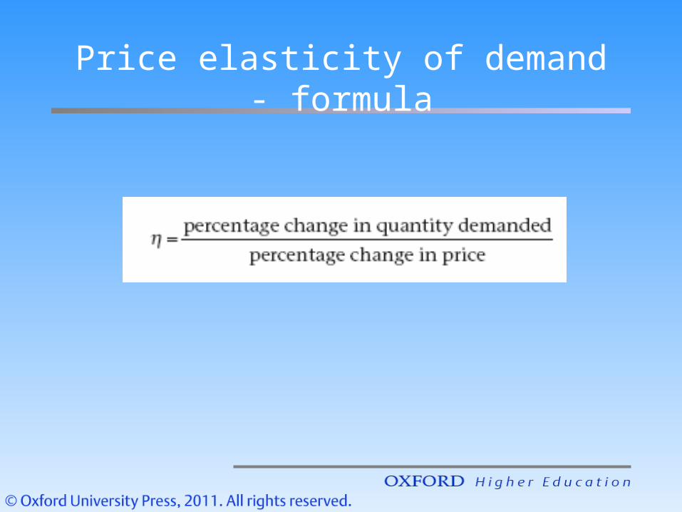
Price elasticity of demand - formula

Calculation of Two Demand Elasticities

Good A

Quantity

Price

Good B

Quantity

Price

100

£1

200

£5

95

£1.10

140

£6

Original New % Change Elasticity

-5%

-10%

-30%

20%

-5%/10% = -0.5%

-30%/20%=-1.5%

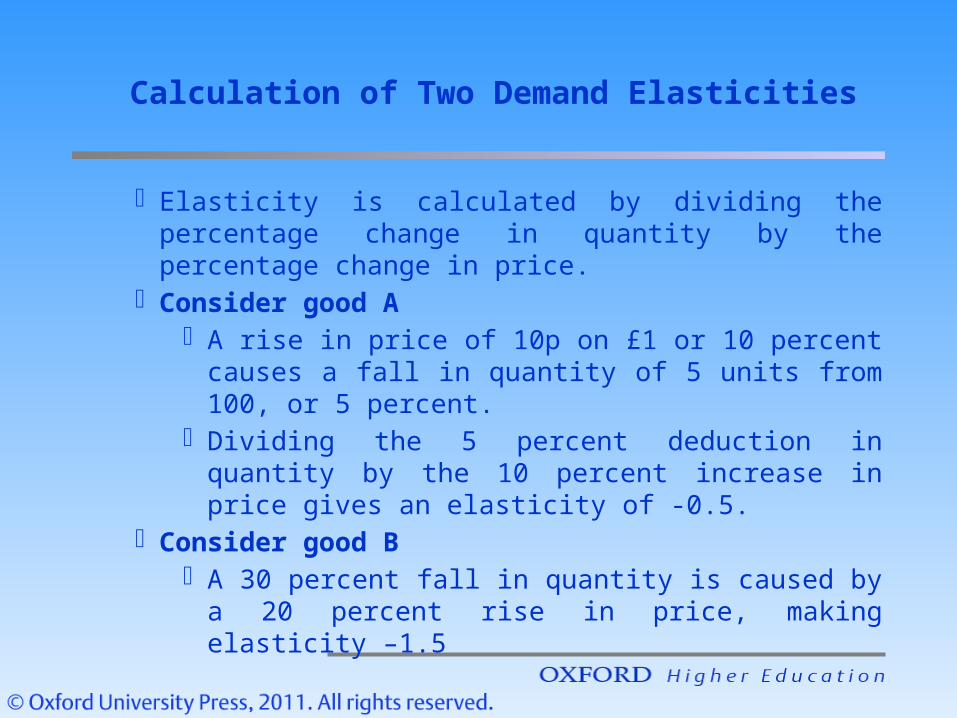
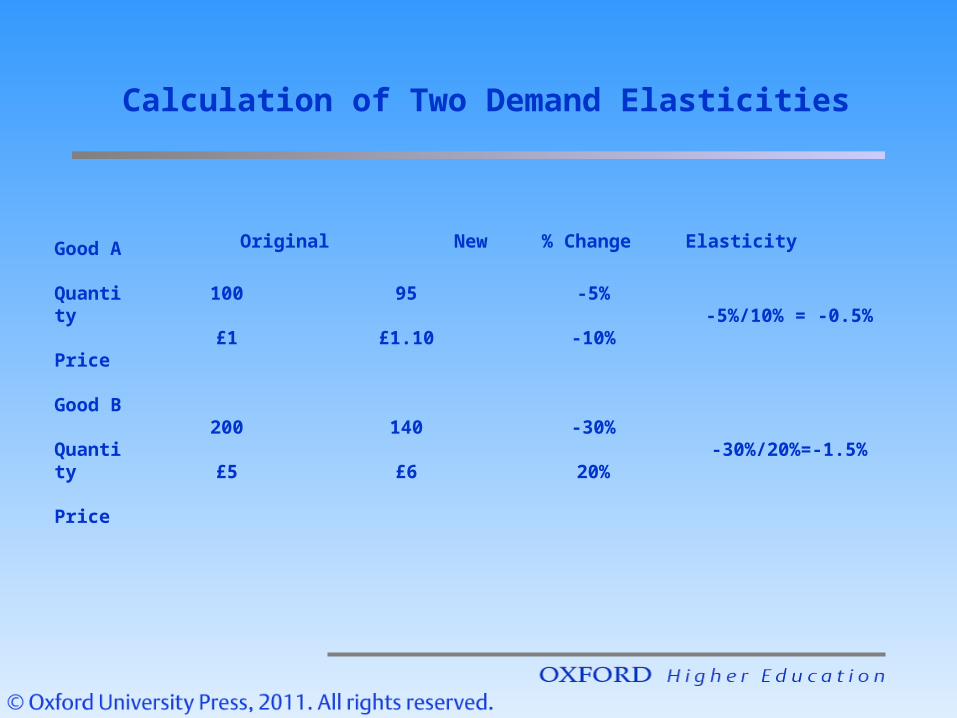
· Elasticity is calculated by dividing the percentage change in quantity by the percentage change in price.

· Consider good A· A rise in price of 10p on £1 or 10 percent causes a fall in

quantity of 5 units from 100, or 5 percent.· Dividing the 5 percent deduction in quantity by the 10

percent increase in price gives an elasticity of -0.5.· Consider good B

· A 30 percent fall in quantity is caused by a 20 percent rise in price, making elasticity –1.5

Calculation of Two Demand Elasticities

Interpreting price elasticity

• The value of price elasticity of demand ranges from zero to minus infinity.

• In this section, however, we concentrate on absolute values, and so ask by how much the absolute value exceeds zero.

• Elasticity is zero if quantity demanded is unchanged when price changes, namely when quantity demanded does not respond to a price change.

• As long as there is some positive response of quantity demanded to a change in price, the absolute value of elasticity will exceed zero. The greater the response, the larger the elasticity.

• Demand is said to be ‘elastic’

• Whenever this value is less than one, however, the percentage change in quantity is less than the percentage change in price and demand is said to be inelastic.

• When elasticity is equal to one, the two percentage changes are then equal to each other.

• This is called unit elasticity.

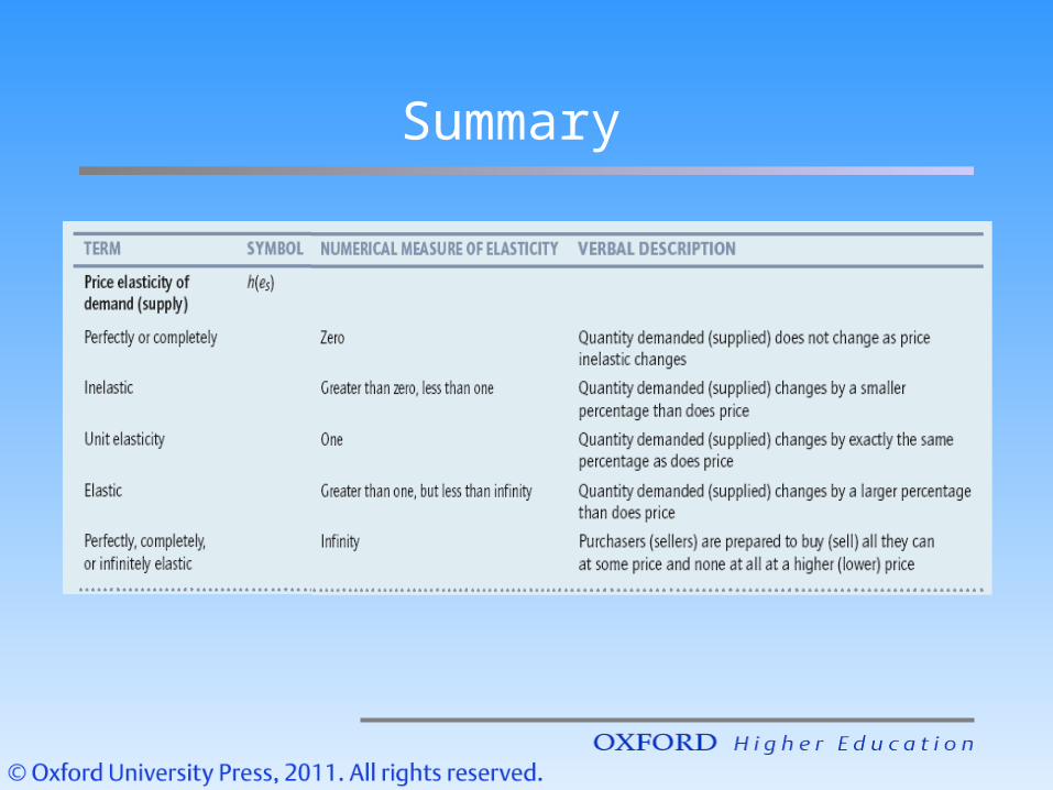
Summary

Note!

– 1. When elasticity of demand exceeds unity (demand is elastic), a fall in price increases total spending on the good and a rise in price reduces it.

– 2. When elasticity is less than unity (demand is inelastic), a fall in price reduces total spending on the good and a rise in price increases it.

– 3. When elasticity of demand is unity, a rise or a fall in price leaves total spending on the good unaffected.

What determines elasticity of demand?

• The main determinant of elasticity is the availability of substitutes.

• Closeness of substitutes—and thus measured elasticity —depends both on how the product is defined and on the time period under consideration.

Note!

A product with close substitutes tends to have an elastic demand; one with no close

substitutes tends to have an inelastic demand.

Quantity

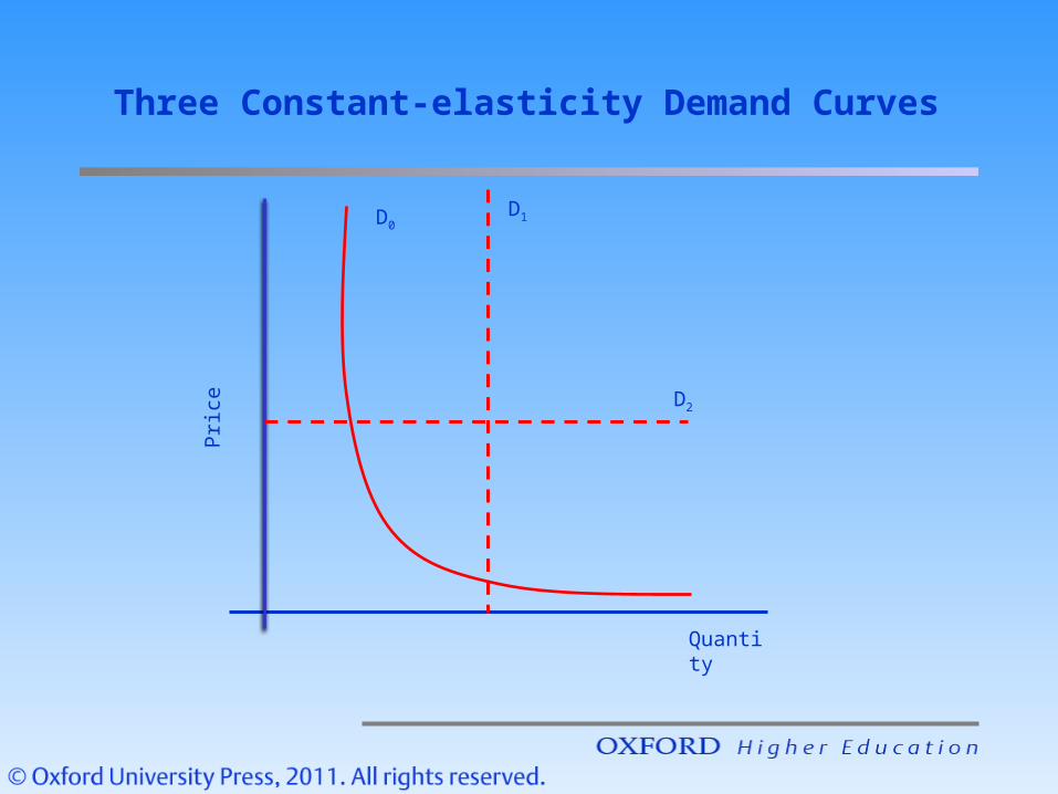
Three Constant-elasticity Demand Curves

Pri

c eD0

D1

D2

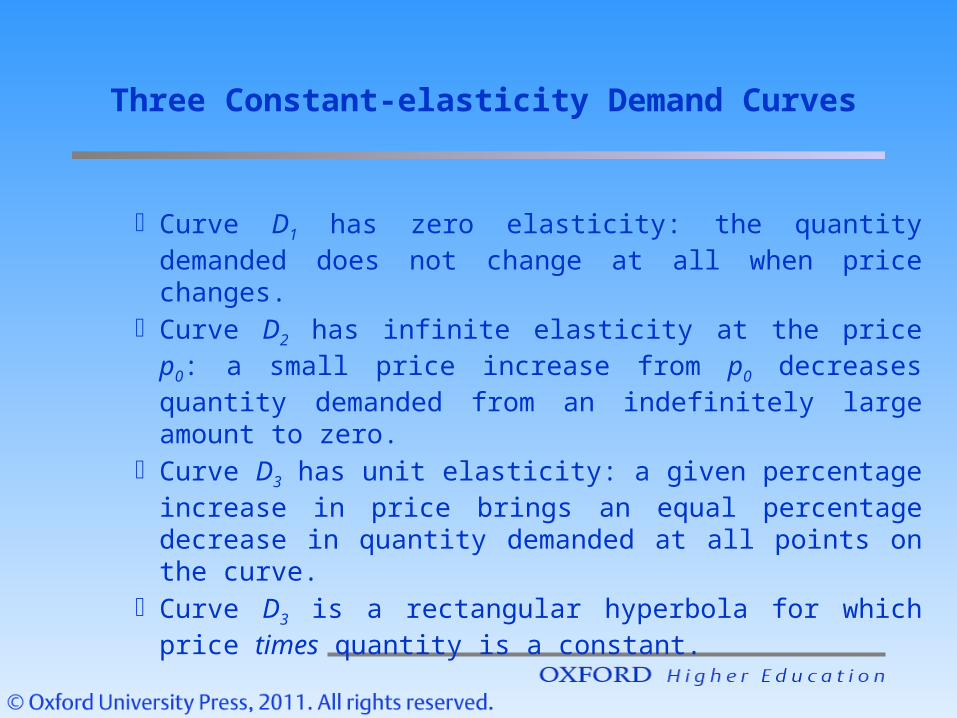
· Curve D1 has zero elasticity: the quantity demanded does not change at all when price changes.

· Curve D2 has infinite elasticity at the price p0: a small price increase from p0 decreases quantity demanded from an indefinitely large amount to zero.

· Curve D3 has unit elasticity: a given percentage increase in price brings an equal percentage decrease in quantity demanded at all points on the curve.

· Curve D3 is a rectangular hyperbola for which price times quantity is a constant.

Three Constant-elasticity Demand Curves

q

p

q

pA

B

D

Pri

ce

Quantity0

Elasticity on a Linear Demand Curve

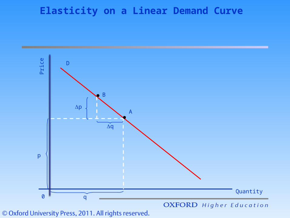
· Starting at point A and moving to point B, the ratio p/q is the slope of the line.

· Its reciprocal q/p is the first term in the percentage definition of elasticity.

· The second term in the definition is p/q, which is the ratio of the coordinates of point A.

· Since the slope p/q is constant, it is clear that the elasticity along the curve varies with the ratio p/q.

· This ratio is zero where the curve intersects the quantity axis and ‘infinity’ where it intersects the price axis.

Elasticity on a Linear Demand Curve

q

p

p1

p2A

Ds

Pri

ce

Quantity

0

Df

p

Two Intersecting Demand Curves

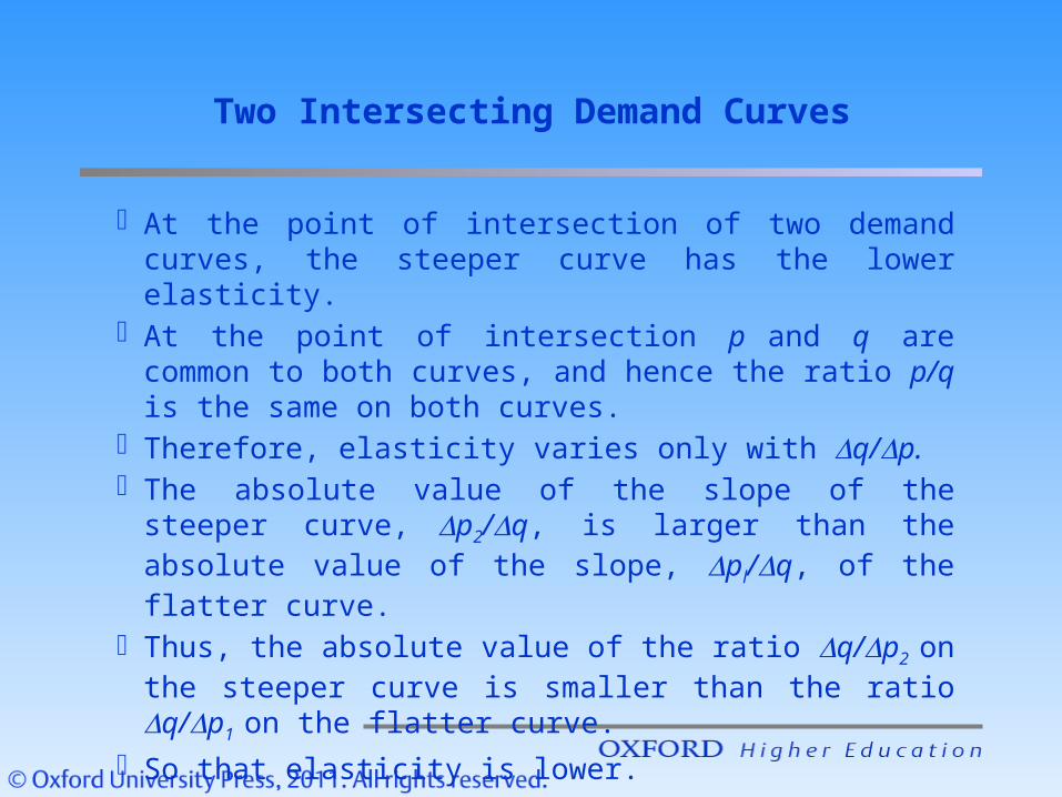
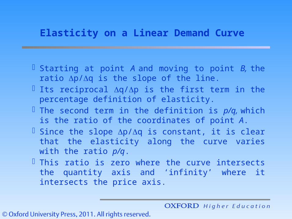
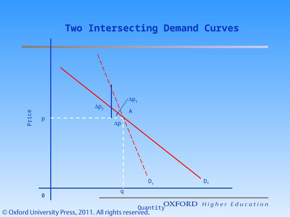
· At the point of intersection of two demand curves, the steeper curve has the lower elasticity.

· At the point of intersection p and q are common to both curves, and hence the ratio p/q is the same on both curves.

· Therefore, elasticity varies only with q/p. · The absolute value of the slope of the steeper curve, p2/q, is

larger than the absolute value of the slope, pl/q, of the flatter curve.

· Thus, the absolute value of the ratio q/p2 on the steeper curve is smaller than the ratio q/p1 on the flatter curve.

· So that elasticity is lower.

Two Intersecting Demand Curves

q

p

D

E

A

B

Pri

ce

Quantity0

C

Demand

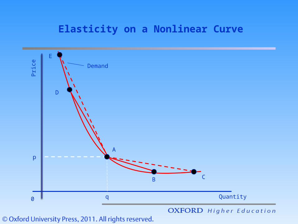
Elasticity on a Nonlinear Curve

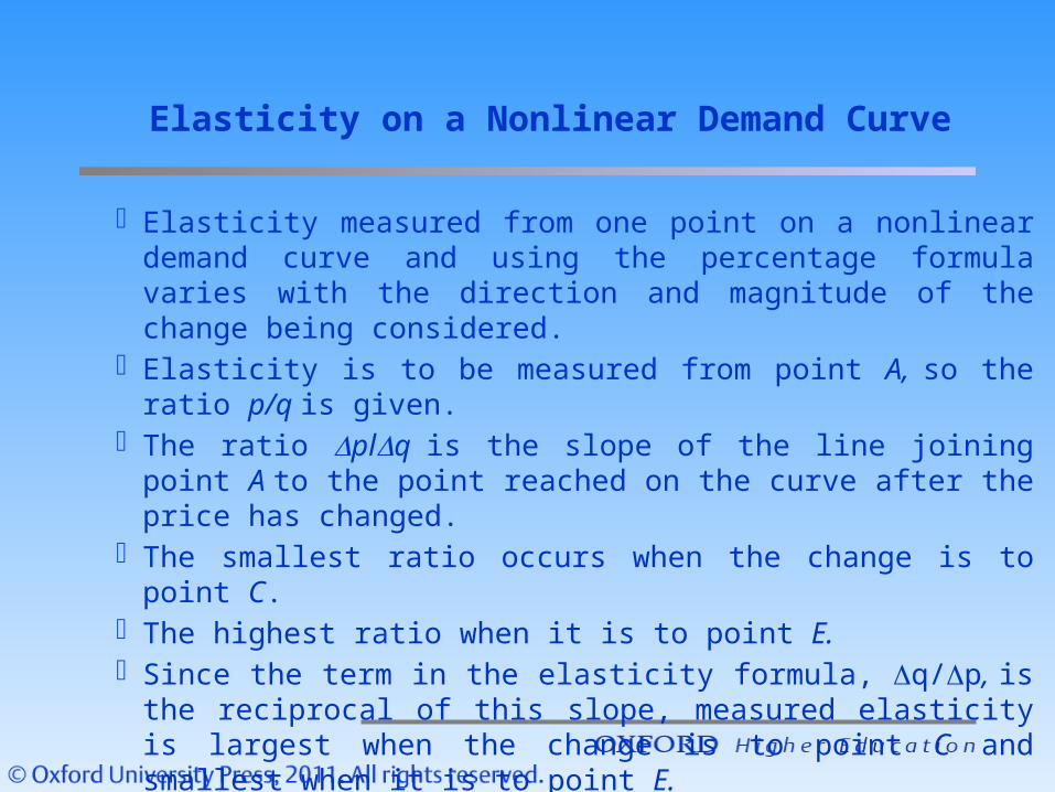
· Elasticity measured from one point on a nonlinear demand curve and using the percentage formula varies with the direction and magnitude of the change being considered.

· Elasticity is to be measured from point A, so the ratio p/q is given.· The ratio plq is the slope of the line joining point A to the point

reached on the curve after the price has changed.· The smallest ratio occurs when the change is to point C.· The highest ratio when it is to point E.· Since the term in the elasticity formula, q/p, is the reciprocal of this

slope, measured elasticity is largest when the change is to point C and smallest when it is to point E.

Elasticity on a Nonlinear Demand Curve

q

p

D

a

b”

Pri

ce

Quantity0

b’

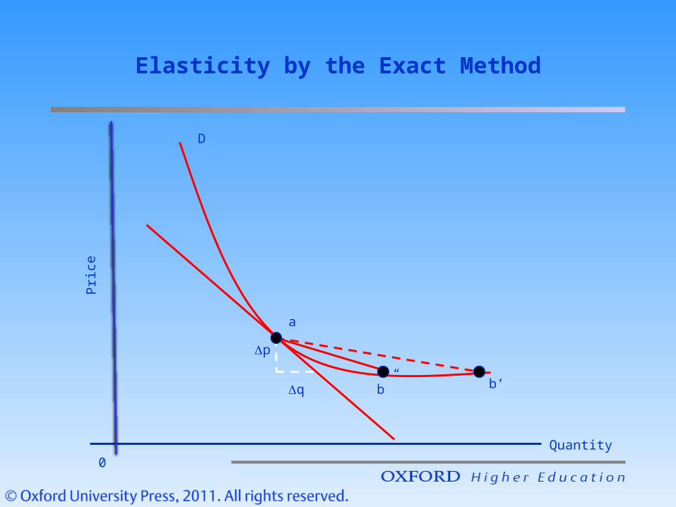
Elasticity by the Exact Method

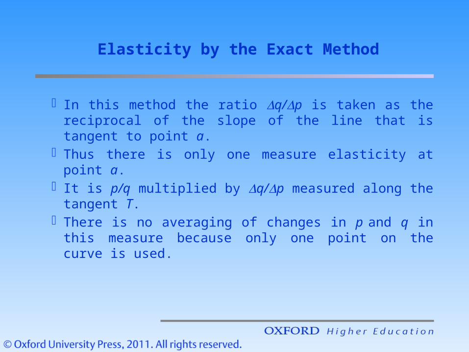
· In this method the ratio q/p is taken as the reciprocal of the slope of the line that is tangent to point a.

· Thus there is only one measure elasticity at point a. · It is p/q multiplied by q/p measured along the tangent T. · There is no averaging of changes in p and q in this measure

because only one point on the curve is used.

Elasticity by the Exact Method

p2

p1

p0

q2 q0q’1q1q’2

E2E’2

E1E’1

E0

Dl

DsoDs1Ds2

Quantity

Pri

ce

Short-run and Long-run Demand Curves

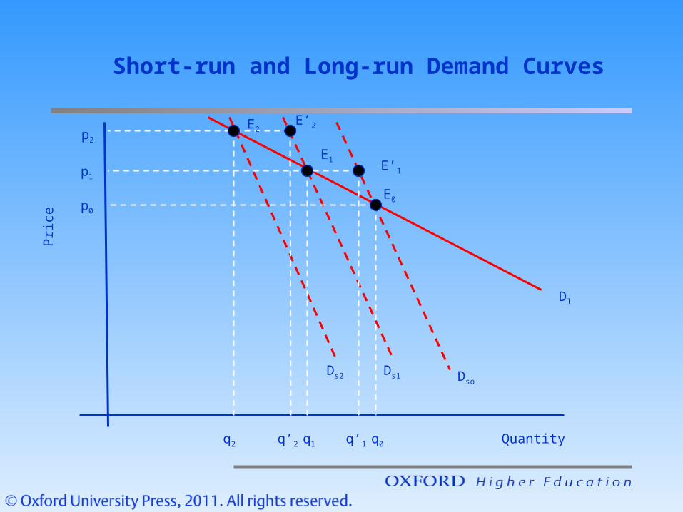
· DL is the long-run demand curve showing the quantity that will be bought after consumers become fully adjusted to each given price.

· Through each point on DL there is a short-run demand curve.

· It shows the quantities that will be bought at each price when consumers are fully adjusted to the price at which that particular short-run curve intersects the long-run curve.

· So at every other point on the short-run curve consumers are not fully adjusted to the price they face, possibly because they have an inappropriate stock of durable goods.

Short-run and Long-run Demand Curves

· For example, when consumers are fully adjusted to price p0 they are at point E0 consuming q0.

· Short-run variations in price then move them along the short-run demand curve DS0.

· Similarly, when they are fully adjusted to price p1, they are at E1 and short-run price variations move them along DS1.

· The line DS2 shows short-run variations in demand when consumers are fully adjusted to price p2.

Short-run and Long-run Demand Curves

Qua

ntit

y

Income0

The Relation Between Quantity Demanded and Income

Qua

ntit

y

y2y10

Zero income elasticity

qm

Income

The Relation Between Quantity Demanded and Income

Qua

ntit

y

Income y2y10

Positive income elasticity

Zero income elasticity

qm

The Relation Between Quantity Demanded and Income

Qua

ntit

y

Incomey2y10

Positive income elasticity

Zero income elasticity Negative income elasticity

[inferior good]

qm

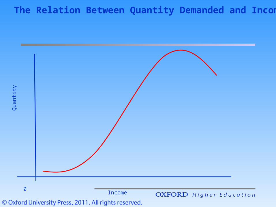
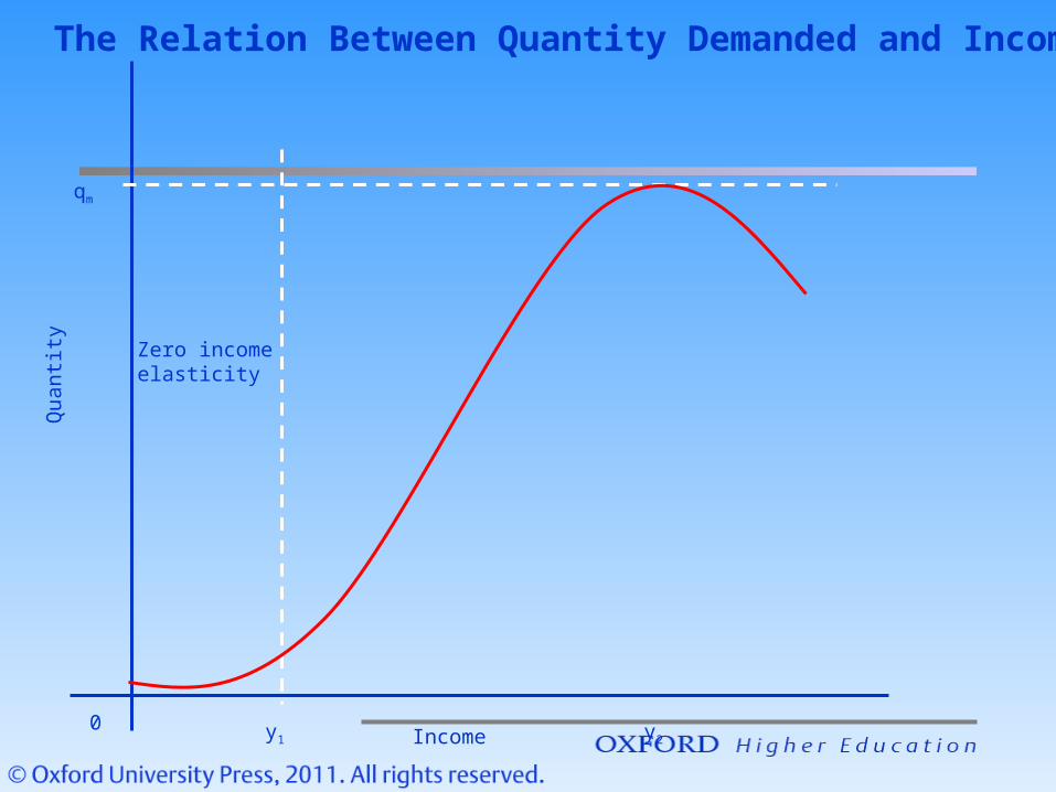
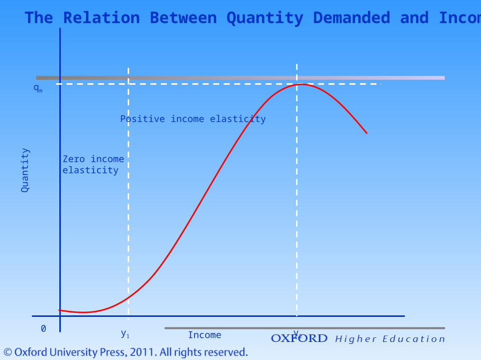
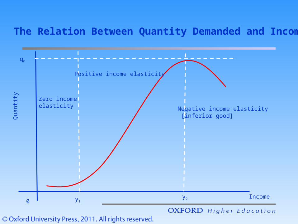
The Relation Between Quantity Demanded and Income

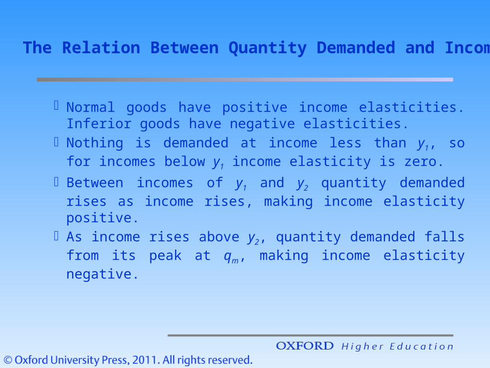
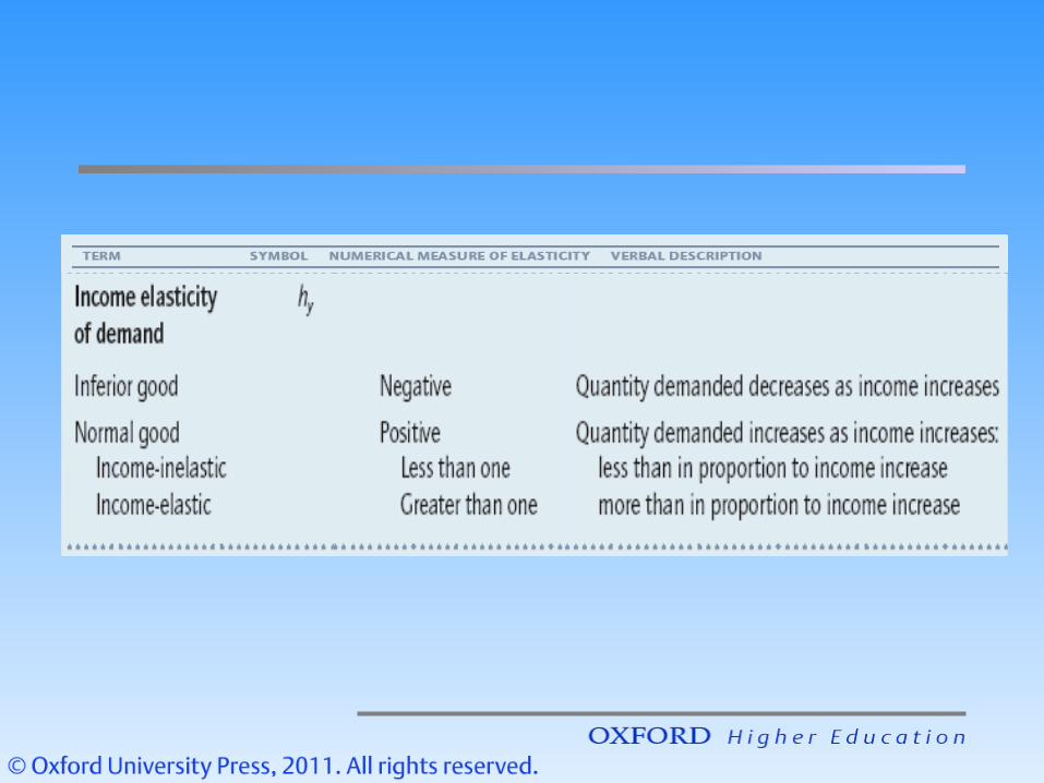
· Normal goods have positive income elasticities. Inferior goods have negative elasticities.

· Nothing is demanded at income less than y1, so for incomes below y1 income elasticity is zero.

· Between incomes of y1 and y2 quantity demanded rises as income rises, making income elasticity positive.

· As income rises above y2, quantity demanded falls from its peak at qm, making income elasticity negative.

The Relation Between Quantity Demanded and Income

Supply elasticity

• We have seen that elasticity of demand measures the response of quantity demanded to changes in any of the variables that affect it.

• Similarly, elasticity of supply measures the response of quantity supplied to changes in any of the variables that influence it.

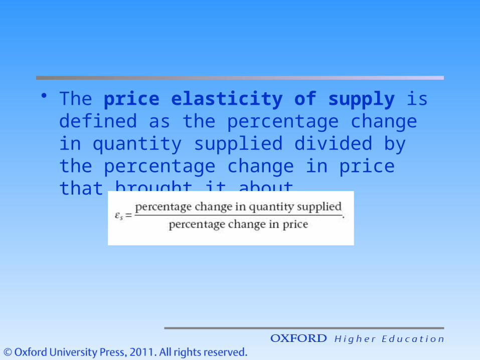
• The price elasticity of supply is defined as the percentage change in quantity supplied divided by the percentage change in price that brought it about.

S1

S2

S3q1

p1

Pri

ce

Pri

ce

Quantity

Quantity

Quantity

Pri

ce

[iii]. Unit Elasticity

[ii]. Infinite Elasticity[i]. Zero Elasticity

Three Constant-elasticity Supply Curves

p

pq

Other demand elasticities

• The concept of demand elasticity can be broadened to measure the response to changes in any of the variables that influence demand.– Income elasticity of demand– Cross elasticity of demand

Income elasticity

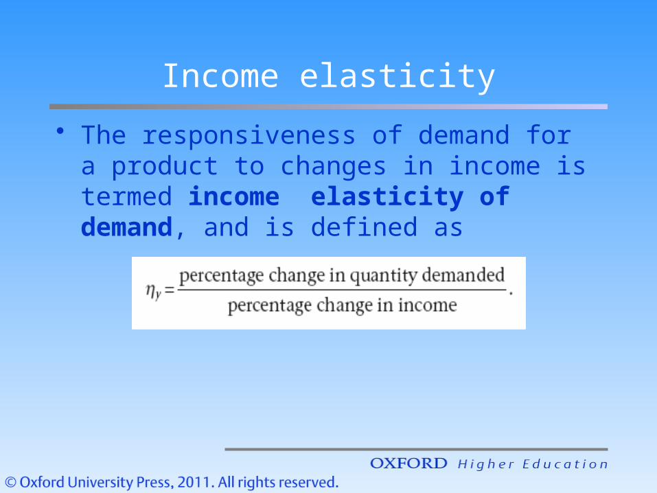
• The responsiveness of demand for a product to changes in income is termed income elasticity of demand, and is defined as

• If the resulting percentage change in quantity demanded is larger than the percentage increase in income, hy will exceed unity.

• The product’s demand is then said to be income-elastic. If the percentage change in quantity demanded is smaller than the percentage change in income, hy will be less than unity.

• The product’s demand is then said to be income-inelastic.

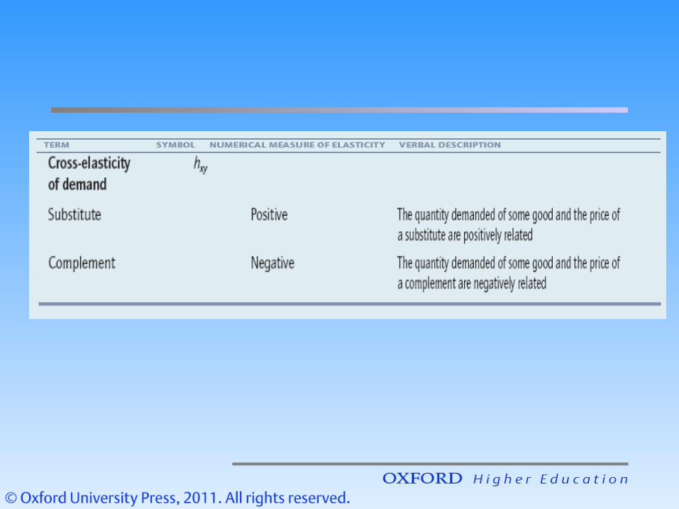
Cross-elasticity

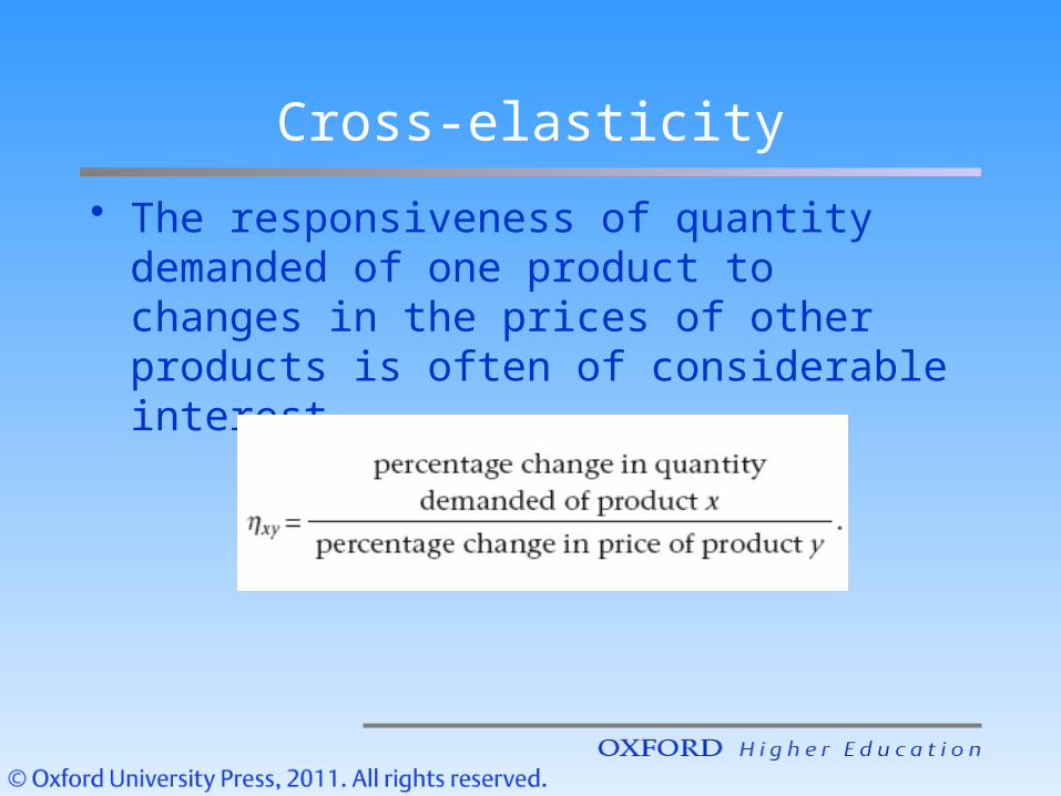
• The responsiveness of quantity demanded of one product to changes in the prices of other products is often of considerable interest.

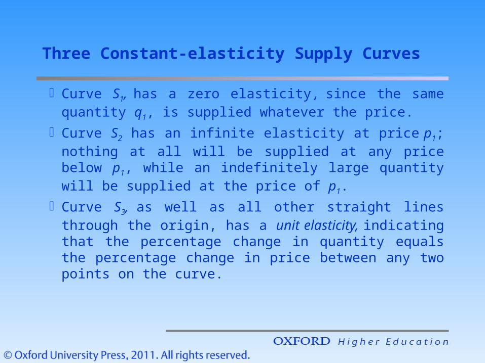
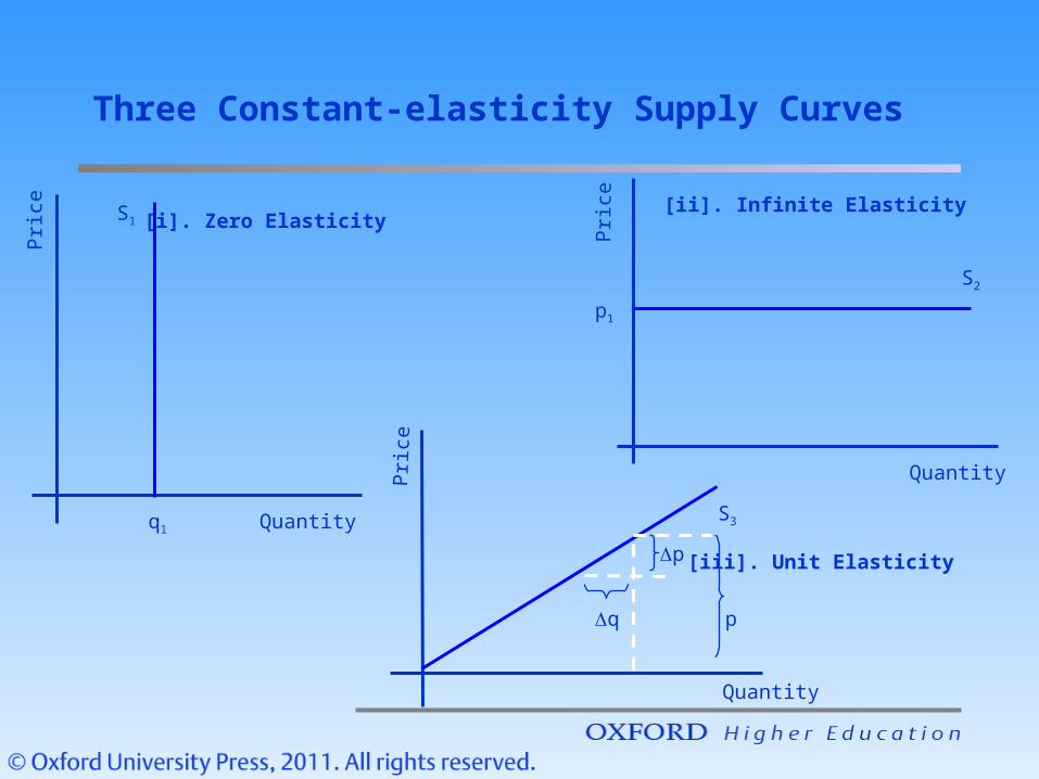
· Curve S1, has a zero elasticity, since the same quantity q1, is supplied whatever the price.

· Curve S2 has an infinite elasticity at price p1; nothing at all will be supplied at any price below p1, while an indefinitely large quantity will be supplied at the price of p1.

· Curve S3, as well as all other straight lines through the origin, has a unit elasticity, indicating that the percentage change in quantity equals the percentage change in price between any two points on the curve.

Three Constant-elasticity Supply Curves

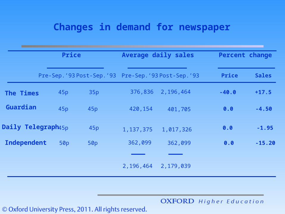
Changes in demand for newspaper

50p

2,179,039

Price Average daily sales Percent change

Pre-Sep.’93 Post-Sep.’93 Price Sales

The Times

Guardian

35p

45p

45p

420,154

362,099

2,196,464

Pre-Sep.’93 Post-Sep.’93

Daily Telegraph

Independent 50p

45p

45p

45p

-15.20

+17.5

-4.50

-1.95

0.0

-40.0

0.0

0.0

376,836 2,196,464

1,137,375 1,017,326

401,705

362,099