Elasticity of rigid networks

Macromolecules Volume 24, Number 24 November 25, 1991

0 Copyright 1991 by the American Chemical Society

Elasticity of Rigid Networks

J. L. Jones’*+ and R. C. Ball

Cauendish Laboratory, Cambridge CB3 OHE, U.K.

Received March 7, 1991; Revised Manuscript Received June 25, 1991

ABSTRACT The elasticity of a network with rigid-rodlike chains is investigated, within a Cayley tree model for the local structure. The length scale down to which the deformations are affine with the bulk is found by renormalization methods, computing the force constants for a chain to translate and rotate relative to the rest of the network. The analysis shows that there is a critical coordination number, corresponding to a second-order phase transition in the elasticity: below this the network rigidity is governed by rod bending alone, and above it is dominated by stretching. The elastic modulus and Poisson’s ratio for this network are also evaluated.

1. Introduction Interest in the properties of rigid networks has arisen

from many sources. A rigid network is one in which the constituent chains have very little flexibility, in contrast to say conventional polymer chains, which are very flexible and so have many different configurations giving rise to properties which are governed by entropy. Two broad classes of materials which can be described as rigid networks are as follows. The synthesis of polymer networks which have very rigid chains as their basic constituents and rigid cross-links have been achieved by Aharoni’ and measurements made of their elastic properties. Silica gels213 have also been interpreted as rigid macromolecular networks. Another class of materials which should display some degree of rigidity are biopoly- mer networks: gels with semirigid chains and physical, temporary cross-link points as discussed in ref 4.

In the work which is presented here, chains are taken to be rigid in the sense that thermal fluctuations in their conformation are small compared to their size and that they are rigidly joined at junction points. The work of deformation, and hence the elastic moduli, is then dominated by molecular elasticity: they are typically tem- perature independent and loosely termed enthalpic. In this regime conventional models for classical flexible and/ or freely hinged networks which rely on the large config- urational entropy are no longer applicable.

The model which we present here treats the network elements as straight rods when undeformed. The rods are then allowed to bend, stretch, translate, and rotate under deformation. The deformation of a single element

+ Present address: Department of Materials Science, Northwestern University, Evanston, IL 60208.

0024-9291/91/2224-6369$02.50/0

is modeled by the case of a rod bending and stretching. We first give the equations describing the deformation of a rod attached to rigid anchors and then separately look a t the case of a rod with flexible anchors modeling its coupling to the background for “affine” deformation in a network. The network structure is modeled as a simply Cayley tree of such elements in order to simplify the calculations.

The Cayley tree provides a convenient way of calculating the elastic constants at different length scales, which is useful for the renormalization process which we perform. Most real networks are expected to have much more complex structures than that of a Cayley tree, and therefore the theory may be limited in its description of these systems. However, it is possible to synthesize some “starburst” polymers which, at least to a certain radius, have quite a well-defined structure which is essentially that of a Cayley tree. If this model is to be tested as a description for real networks, then networks composed of starburst clusters may provide a starting point for investigations.

We are interested in the values of the anchor force constants which govern how easily the network elements can undergo translations and rotations relative to the mean and hence how resistant the whole network is to deformation. From the single-rod equations we derive recursion relations between the force constants a t consecutive levels of the Cayley tree. Fixed points of these govern the network elasticity; their stability-how rapidly they are approached-is interpreted as a measure of how close to affine the local deformation will be.

Previous models of the elastic properties of networks with rigid chains and rigid elements can be found in Kan- tor and Webman,6 Brown: Jones and Marques? and Doi and Kuzuu.8 These all rely on assigning an energetic elastic energy term to the chains and calculating the scaling of

0 1991 American Chemical Society

6370 Jones and Ball

a)

-Macromolecules, Vol. 24, No. 24, 1991

ances for bend and twist are equal, these simplify to

GI

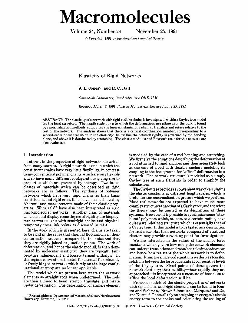
Figure 1. (a) A rod which is rigidly clamped a t the left-hand end. The deformation caused by the applied force and couple F, and G, a t the right-hand end are X, and 6,. (b) A rod with flexible anchors. The left-hand end of the rod is now allowed to translate and rotate and has a translation XI and rotation 61. The motion is resisted by a force Fl = -klX1 and a couple GI = -m161 which reflect the forces and couples which the rest of the network exerts on the end of the rod.

the elastic modulus with the concentration of polymer in the system. Entropic models have been used by Edwards? BOG, Edwards, and Vilgis,"J and Thorpe and Phillips" for networks where the constituent elements are rigid but where the cross-links are freely hinging. Also models by Doi and Kuzuu8 have been used to describe the case where there is not a fixed number of cross-links.

In the elastic behavior of a network, a central issue is at what length scale, if any, the local elastic constants of the network accurately describe that of a bulk sample of material. The crudest assumption to use in any model for networks is that the deformation is affine down to a length scale of the order of one rod length; i.e., the elastic constants which apply to the movement of a single rod with flexible anchors are the same as for a network of such rods. However, we are able to show that this may not be a very accurate approximation, and we investigate which length scale may be taken as the mesh size for the system. Renor- malizing the force constants show that this depends on the value of the functionality z , the spatial dimension d , and how much the rod is allowed to stretch as well as to bend.

In light of these results, the aims of the later sections of this paper will be to calculate the stress in a deformed network and hence its modulus and Poisson's ratio. The initial sections of this paper will deal with rods which are only allowed to bend, and the more general case where both stretch and bend are considered will be addressed in the later sections.

2. Single-Rod Equations We first consider the deformation of a single rod,

clamped by a rigid anchor at one end and with a force F, and a couple G, applied at the other end as in Figure la. The amount of deformation which the right-hand end of the rod undergoes may be described in terms of the displacement X, and the angle of rotation 6, of the end of the rod. If the rod can only bend and twist, then 6, and X, are related to the force and the couple by the well- known bend equations for a rod: when the local compli-

s2G, A t s3P.F, x,=se, A t---- 27 63'

S S2

Y 27 6, = -G, + -t A F,

where P is a tensor defined by

P-F, = (t A F,) A t (3) Here y is the bend rigidity constant, s is the length of the chain, and t is the direction of the tangent vector along the rod before any displacement occurs. We now want to consider the case of a single rod deforming where the ends of the rod are attached to flexible anchors (Figure lb), with the eventual aim of modeling a rod anchored by the rest of the network. I t will be assumed that the force- displacement law is a simple linear one which can be split into a restoring force and a restoring couple. For example, at the left-hand end of the rod then Fl = -KIXI and the couple is G I = -M181. Once we have the equations relating X, and 6, to the force constants a t the other end, KI and MI, then a self-consistent calculation will be performed in order to determine the force constants for a network made up of such rods. The equations giving the two displace- ments, angular and translational, i.e., for Xr and 8, for the case of flexible anchors, are

s2G, A t s3P-F, (4)

Fr K, 27 67

x,=-++e, A t----

We can define new variables which are dimensionless so that we eliminate y and s from the equations. Since there is only one length scale s, this sets the scale for all lengths, y / s for all torques, and y/s2 for all forces, and we scale all the other variables in terms of them; Le., ml = s M I / ~ , k1= s3Kl/y, = Xr/S, g, = sGr/Y and f, = s2F,/y. The angle 8, is dimensionless and is not changed. The new versions of (4) and (5 ) with dimensionless variables are

and (6) can be rewritten so that the displacement Xr is expressed in terms of f, and g, only as follows:

The quantities ml and kl are the force constants which mechanically couple one end of the rod to the rest of the network and clearly represent an average or mean-field effect. Deformation of rods locally may be quite different from the overall strain in the network, as is seen in the extreme case of an inextensible rod initially aligned along a principle axis in pure extension. Such cases clearly show up in turn as anomalies in the true local values of ml and kl felt by the neighboring rods and hence in their deformation also, and so on. Such effects may blow up at large scales, and just how far they do propagate is explored in the next sections, together with limiting average values

Macromolecules, Vol. 24, No. 24, 1991

of the force constants from which we will subsequently calculate the macroscopic elastic constants.

3. Renormalization of the Force Constants, To Determine Their Values at Different Length Scales of the Network

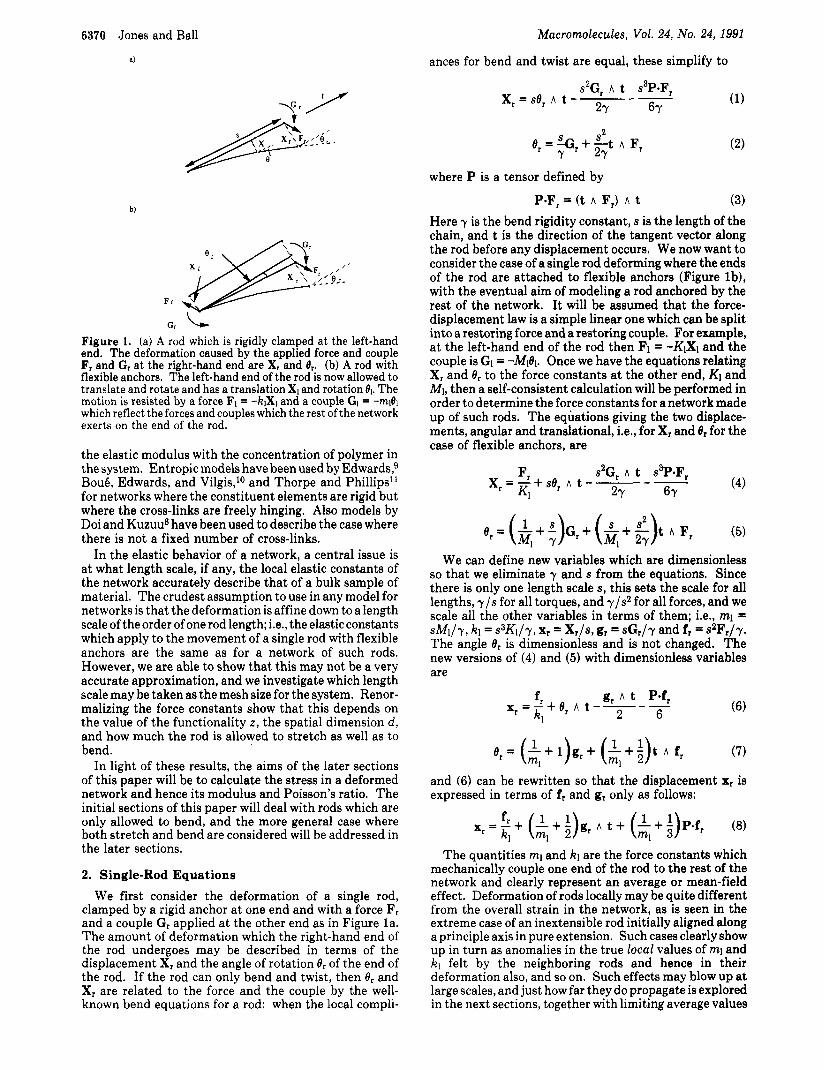
We can renormalize the forces and couples by expressing the values a t one branch point in terms of the values at branch points a t the next level down the tree and derive a value for kl and ml a t every step n. Referring to Figure 2, the calculation is as follows. The total force at a branch point V will be the sum of the forces a t the ends of the z rods, joining at V, and will be zero at equilibrium. Similarly for the total couple a t V we must add together the couples acting at the ends of all z rods and equate them to zero. I t is therefore straightforward to determine any one of the f% at V if the other z - 1 forces are known. In particular, we want to find the force on the left-hand end of a rod which is part of the next generation in the Cayley tree structure which is f( and so

Elasticity of Rigid Networks 6371

1

and similarly

gi' = -cg,'" 1

(10)

f{ and g( are the force and the couple on the left-hand end of a rod of the next generation of the Cayley tree. The couples a t different ends of a rod are related by gl + gr + t A f, = 0. A t a junction the displacement and the rotation for each rod are the same, although the force and the couple which each contributes will be different. We can therefore write xr and 8, in terms of any of the i rods' equations as follows

These equations can be inverted to give the fr") and g P in terms of the e,, x,, and t(i). Therefore

where

We now wish to find actual expressions for the force and couple in (9) and (10) and to set up recursion relations for them. This requires the substitution of (13) and (14) into (9) and (10). The sum is performed over all the ( z - 1) rods going into the junction. From the above expressions it can be seen that f,(i) and g,(i) both contain a t(i)

Figure 2. Renormalization of the forces. The figure shows parta of two of the layers of the Cayley tree. The forces which are applied to the ends of the first generation of rods are f+, f?, ft, etc. There must be forces frl, ft , and f,3 acting at the right-hand end of the rods, Le., at V where fp) = -f,c'). For equilibrium of the forces at V it must follow that f{ = -xf$) where f{ is the force which acta on the left-hand end of the rod VY.

dependence. The force is Cifr(i) and so will be a function of all the t(')s of the rods coming into that junction and will be a fairly complicated expression.

At this point we introduce a simplifying assumption, and we say that the sum of the ( z - 1) forces a t V is approximately ( z - 1) times the value of the force at V averaged over all possible t(i) directions, so that

This is effectively assuming that there are a sufficiently large number of rods entering each junction point that their effect may be considered isotropic. In section 7 a closer look is taken at this assumption by measuring the spread in the values of 121 and ml around the average values and it is shown to be a fairly good approximation. We can treat the g,(i)s in exactly the same way. The average force and couple are found by averaging over all possible t%. The averaging is performed in three dimensions and is assumed to be isotropic. We are interested in the average force rather than the average displacement since at the junction all the rods share a common displacement. By finding the average force and couple we are finding ( fr) = - ( k , ) x , and likewise (g,) = -(m,)&. These are related to the constants for the next layer by f{ = - (z - 1) ( f r ) = -k{x{ and g{ = -(z - 1) ( gr) = -m{8{. The averaged values of the force constants a t V, Le., after one step, are

m,' = - (z - l ) ( m r ) = ( z - 1) 1 + - (

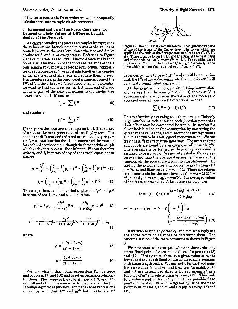
If we wish to find any other kln and mf, we simply use the above recursion relations to determine them. The renormalization of the force constants is shown in Figure 3.

We now want to investigate whether there exist any stable fixed points for the coupled set of equations (18) and (19). If they exist, then, a t a given value of n, the force constants reach fixed values which remain constant with larger length scales. We may solve for the fixed point force constants k* and m* and then test for stability. k* and m* are determined directly by expressing k* as a function of m* and substituting back into (19). This leads to a cubic equation for m*, giving three possible fixed points. The stability is investigated by using the fixed point solutions for kl and ml and simply iterating (18) and (19).

6372 Jones and Ball Macromolecules, Vol. 24, No. 24, 1991

We can now treat the x, and 8, equations in the same way as before. The inverted form of ( 2 2 ) is

k~ m (

Figure 3. (a) Renormalization of the force constants kl and ml. The diagram shows the renormalization scheme. The structure on the left with the force constants kl and ml acting at the ends of the two rods as shown can be represented as a single rod with the renormalized force constants k{ and mi acting at its end. (b) Two steps in the renormalization of the force constants are shown.

Performing the above gives three classes of results which are distinguished by different regions of z. Solving for the fixed point leads to

(20) from which it can be seen that a finite fixed point only exists for 2 < z C 4 . The case z = 2 gives a fixed point with zero modulus, and for z I 4 it is necessary to allow some stretching of the rods as well as bending in order to arrive at finite values.

k*P* = 3 ( 2 - z ) / ( z - 4)

4. Force Constants for Rods Which Can Stretch and Shear

We can next consider the effect of allowing the rods to stretch and to shear. We assign to eachrod a finite modulus for stretching which we denote by KII. In addition the rods have a shear modulus KI. The effect of these extra degrees of freedom can easily be incorporated into the above equations. To (4) we must add the contributions to the displacement, from both the stretching and shearing of the rod. Therefore, we can rewrite (4) as

and the equation for 8, is unchanged. The above equation can again be expressed in reduced variables as before if in addition we use kll = Kils3/y and k l = Kls3/y. Rewriting (21) in this way gives

Further investigation of these expressions shows that the value of k l has a negligible effect on the values of k* and m*, since any deformation which is required perpen- dicular to the rod axis can be accommodated by bending more easily than by shearing. Therefore in all that follows we set k l = m and neglect its effect.

where

and the equation for gr(i) is as it was in section 3 , i.e., is given by (14). Equation 23 can then be averaged over all possible values of t(i) to obtain an expression for the force constant k f .

The expressions for k f and mi therefore become

m,' = -(z - l)(m,) = ( z - 1) 1 + - ( $x

the expression for mf being the same as for the bending only case.

5. Results for the Fixed Points In this section we shall discuss how the fixed point varies

ford = 3 dimensions as a function of z for different values of kll. The results fall into three distinct regions.

(i) ( z - 1) < 3. Finite stable fixed points in kl and ml exist, for all values of kll. In this region the deformation is dominated by bending. For kll= 0) (25 ) and ( 2 6 ) reduce to (18) and (19). Even for the infinite kll case, finite fixed points in the force constants exist, showing that the deformation is dominated by bending.

If z = 2 , both force constants kl and ml tend to a fixed point a t zero. For z = 2 the network is connected as a line. Consequently each iteration step simply adds a length s to the length of the system without introducing any additional branching of the rods. The amount of bending deformation of a rod for a given force scales with s3, its length cubed. I t is consistent therefore that, as thenumber of iterations is increased, then the force constants for effectively linear chains should decrease toward zero.

(ii) ( z - 1) = 3. Finite stable fixed points only exist if the rods are allowed to stretch as well as bend.

Without stretch (infinite k l l ) kl tends toward infinity linearly with the number of iterations: if (18) is rewritten for large kl, but retaining terms to first order in l/& we obtain

k,' = k , + 2 / P ( 2 7 ) and for large values of kl, then ml and P are constant.

When stretch is included, a finite fixed point does exist and the value can be extracted from ( 2 5 ) and (26 ) . We focus our attention on rods of a large axial ratio for which PklI - (s /w)2 >> 1, where s and w are the respective rod length and diameter and @ is bounded by 1/12 < p < 113. If also klP >> 1, (25) may be rewritten as

k,' = - (' - "( 1 - f + F) (1 - 6) ( 2 8 ) P


Growth o! k for 2=4


Growth of k for 2=5

O 1 ' I ' , ' , ' ,

0 y,,,,,,.,.I 20 40 60 80 100

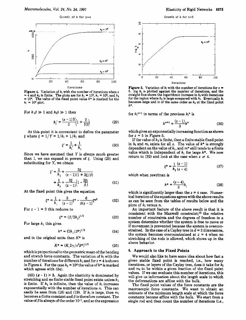
Iterations Figure 4. Variation of kl with the number of iterations when z = 4 and kI is finite. The plots are for k , = lo2, kll = lo3, and kll = 104. The value of the fixed point value k* is marked for the k,l = 104 plot.

For kllp >> 1 and k@ >> 1 then

At this point it is convenient to define the parameter 5 where f = 1/Y = l / k l + f/kll and

1 1 r = q + q (30)

Since we have assumed that Y is always much greater than 1, we can expand in powers of 5. Using (29) and substituting for Y, we obtain

A t the fixed point this gives the equation

For z - 1 = 3 this reduces to

5* = ( P / 2 q ' 2 (33)

k* = (2kl,/P*)'/2 (34)

K* = ( ~ ~ ~ 2 ~ / ~ 3 p ) 1 / 2 (35)

For large K I I this gives

and in the original units then K* is

which is proportional to the geometric mean of the bending and stretch force constants. The variation of kl with the number of iterations for different kll and for z = 4 is shown in Figure 4. For the case kll = lo4 the value of k* is marked which agrees with (34).

(iii) (z - 1) > 3. Again the elasticity is dominated by stretching and no finite stable fixed point exists unless kll is finite. If kll is infinite, then the value of kl increases exponentially with the number of iterations n. This can easily be seen from (18) and (19). If kl is large, then ml becomes a finite constant and P is therefore constant. The value of P is always of the order lO-l, and so the expression

01 ' I ' I ' 1 ' I ' I 0 20 40 60 80 100

Iterations

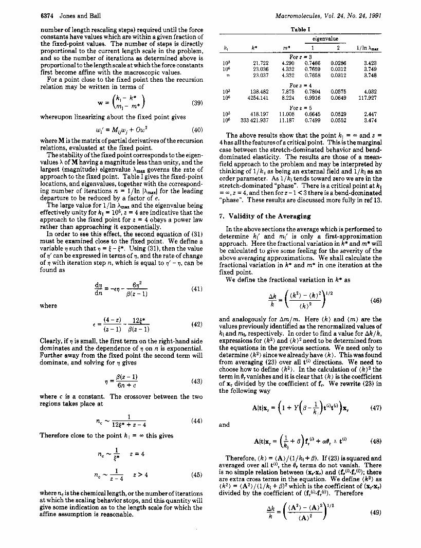
Figure 5. Variation of kl with the number of iterations for z = 5. log kl is plotted against the number of iterations, and the straight line shows the logarithmic increase in kl with iterations for the region where kl is large compared with kl. Eventually kl becomes large and is of the same order as kl at the fixed point k*.

for kp+l in terms of the previous kin is

which gives an exponentially increasing function as shown for z = 5 in Figure 5.

If the value of kll is finite, then a finite stable fixed point in kl and ml exists for all z. The value of k* is strongly dependent on the value of kll, and m* still tends to a finite value which is independent of kll for large k*. We now return to (32) and look at the case when z # 4.

which when rewritten is

(37)

which is significantly larger than the z = 4 case. Numer- ical iteration of the equations agrees with the above results as can be seen from the tables of results below and the plots of kl versus n.

An important feature of the above result is that it is consistent with the Maxwell constraint;12 the relative number of constraints and the degrees of freedom in a system determine whether the system is free to move or if movement is prevented because the system is overconstrained. In the case of a Cayley tree in d = 3 dimensions, the system becomes overconstrained a t z = 4 when no stretching of the rods is allowed, which shows up in the above behavior.

6. Approach to the Fixed Points We would also like to have some idea about how fast a

given stable fixed point is reached, Le., how many iterations, or layers of the Cayley tree, does it take for kl and ml to be within a given fraction of the fixed point values. If we can evaluate this number of iterations, this will give u5 information about the length scale to which the deformations are affine with the bulk.

The fixed point values of the force constants are the macroscopic force constants. We want to obtain an estimate of the minimum length scale a t which the force constants become affine with the bulk. We start from a single rod and then count the number of iterations (i.e.,

6374 Jones and Ball

number of length rescaling steps) required until the force constants have values which are within a given fraction of the fixed-point values. The number of steps is directly proportional to the current length scale in the problem, and so the number of iterations as determined above is proportional to the length scale at which the force constants first become affine with the macroscopic values.

For a point close to the fixed point then the recursion relation may be written in terms of


w = (4- k* ) m,- m* (39)

whereupon linearizing about the fixed point gives

w/ = Mijwj + Ow2 (40) where M is the matrix of partial derivatives of the recursion relations, evaluated a t the fixed point.

The stability of the fixed point corresponds to the eigenvalues A of M having a magnitude less than unity, and the largest (magnitude) eigenvalue A,, governs the rate of approach to the fixed point. Table I gives the fixed-point locations, and eigenvalues, together with the corresponding number of iterations n = l / ln lAmaxl for the leading departure to be reduced by a factor of e .

The large value for l / ln A,, and the eigenvalue being effectively unity for kl l = lo6, z = 4 are indicative that the approach to the fixed point for z = 4 obeys a power law rather than approaching it exponentially.

In order to see this effect, the second equation of (31) must be examined close to the fixed point. We define a variable q such that q = f - f * . Using (31), then the value of q' can be expressed in terms of q, and the rate of change of q with iteration step n, which is equal to q' - q, can be found as

where

(41)

Clearly, if q is small, the first term on the right-hand side dominates and the dependence of q on n is exponential. Further away from the fixed point the second term will dominate, and solving for q gives

P(z - 1) q=- 6n + c (43)

where c is a constant. The crossover between the two regions takes place a t

1 nc - 12€* + z - 4

Therefore close to the point kll = 03 this gives

(44)

(45)

where n, is the chemical length, or the number of iterations at which the scaling behavior stops, and this quantity will give some indication as to the length scale for which the affine assumption is reasonable.

Table I eigenvalue

k I1 k* m* 1 2 l / ln A,

F o r z = 3 103 21.722 4.290 0.7466 0.0286 3.423 106 23.036 4.332 0.7659 0.0312 3.749

m 23.037 4.332 0.7658 0.0312 3.748

Forr = 4 103 138.482 7.875 0.7804 0.0575 4.032 106 4254.141 8.224 0.9916 0.0649 117.927

FOrZ=5 103 418.197 11.008 0.6645 0.0529 2.447 lo6 333 421.937 11.187 0.7499 0.0552 3.474

The above results show that the point kll = m and z = 4 has all the features of a critical point. This is the marginal case between the stretch-dominated behavior and bend- dominated elasticity. The results are those of a mean- field approach to the problem and may be interpreted by thinking of l /k, l as being an external field and l/kl as an order parameter. As l/kl tends toward zero we are in the stretch-dominated "phase". There is a critical point a t kll = m , z = 4, and then for z - 1 < 3 there is a bend-dominated "phase". These results are discussed more fully in ref 13.

7. Validity of the Averaging

In the above sections the average which is performed to determine k( and m i is only a first-approximation approach. Here the fractional variation in k* and m* will be calculated to give some feeling for the severity of the above averaging approximations. We shall calculate the fractional variation in k* and m* in one iteration at the fixed point.

We define the fractional variation in k* as

and analogously for Am/m. Here (k ) and (m) are the values previously identified as the renormalized values of k1 and mi, respectively. In order to find a value for Aklk, expressions for ( k2) and ( k)2 need to be determined from the equations in the previous sections. We need only to determine ( k2) since we already have (k) . This was found from averaging (23) over all t(') directions. We need to choose how to define (k'). In the calculation of (k)' the term in 8, vanishes and it is clear that (k ) is the coefficient of Xr divided by the coefficient off,. We rewrite (23) in the following way

A{tJxr = ( 1 + Y(P-:)t"'t"')x, (47)

and

Therefore, ( k ) = ( A ) / ( l / k l + P ) . If(23) issquaredand averaged over all t(i), the 8, terms do not vanish. There is no simple relation between (Xr-Xr) and (fr'i).fr'i)); there are extra cross terms in the equation. We define ( k 2 ) as ( k 2 ) = (A2)/(1/k1 + p)2 which is the coefficient of (Xr'X,) divided by the coefficient of (f>).f>)). Therefore

(49)


Table I1 z scaling of modulus Am*/m* Ak*/k*


bend dominated 3 E - nyls 0.44 0.71 marginal CBBB 4 E - n(yklp)1/2 0.48 1.41 stretch dominated 5 E - nklp2 0.47 1.41

and

B' p a) Initial position of the rod b) Two halves are deformed affmely

giving

The same approach can be used to find Am/m. Re- ferring back to (14), this may be rewritten in the form

where

B(t)8, = g,(i) + (53)

and

(54)

Again we have to choose how to define ( m2). Equation 14 is squared and averaged over all possible Ns. The value of ( m2) is defined as the coefficient of 8,4, divided by the coefficient of g,Ci)-g,(i). Performing these steps gives

2 (B') - (B)' = 59'

Am*

(55)

(56)

(57)

where

(58)

The actual size of these fractional variations will depend on the values of z and kll, and important selected cases are given in Table 11.

Table I1 contains values of the fluctuations in the renormalized parameters under one iteration at the fixed point calculated in the text, in the limit of large kll. The values above are for k, = IOs, and n is the number density of rods.

8. Stress in a Rigid Network In this section we calculate the network stress, by

considering the stress on a single rod in the bulk, including in the calculation the fact that the deformation of the single rod is not affine with the bulk. The general formula for the network stress is

m*(l + B*k*) k*a*'(l + m*)

U =

(59)

F(i) is the force transmitted down the rod and t(') its

c) The ends of the two halves of the rod have forces and couples applied so that the ends are brought into contact agarn.

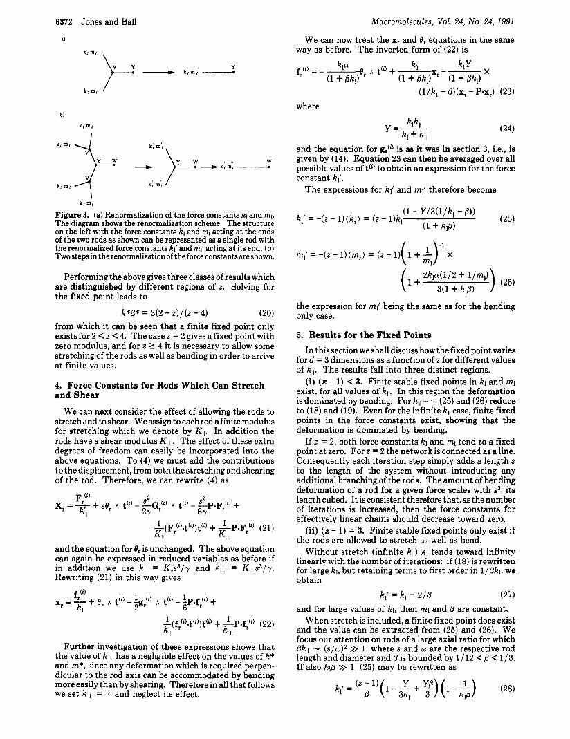
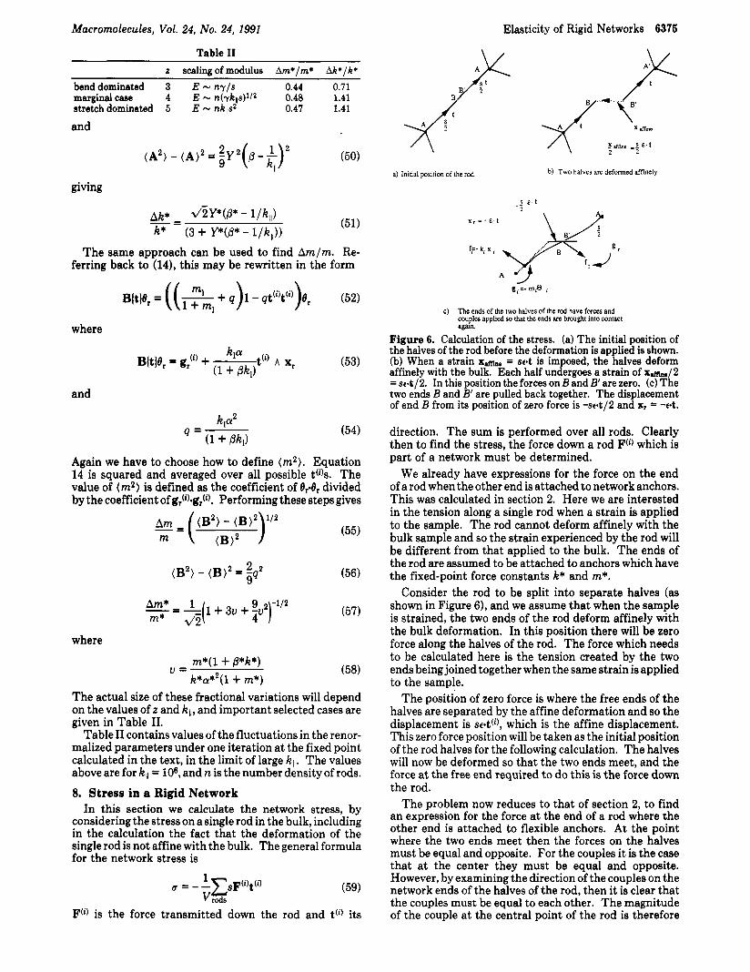
Figure 6. Calculation of the stress. (a) The initial position of the halves of the rod before the deformation is applied is shown. (b) When a strain xam. = set is imposed, the halves deform affinely with the bulk. Each half undergoes a strain of x a e / 2 = st.t/2. In this position the forces on B and B' are zero. (c) The two ends B and B' are pulled back together. The displacement of end B from ita position of zero force is -st.t/2 and xr = -et.

direction. The sum is performed over all rods. Clearly then to find the stress, the force down a rod F(') which is part of a network must be determined.

We already have expressions for the force on the end of a rod when the other end is attached to network anchors. This was calculated in section 2. Here we are interested in the tension along a single rod when a strain is applied to the sample. The rod cannot deform affinely with the bulk sample and so the strain experienced by the rod will be different from that applied to the bulk. The ends of the rod are assumed to be attached to anchors which have the fixed-point force constants k* and m*.

Consider the rod to be split into separate halves (as shown in Figure 6), and we assume that when the sample is strained, the two ends of the rod deform affinely with the bulk deformation. In this position there will be zero force along the halves of the rod. The force which needs to be calculated here is the tension created by the two ends being joined together when the same strain is applied to the sample.

The position of zero force is where the free ends of the halves are separated by the affine deformation and so the displacement is stet('), which is the affine displacement. This zero force position will be taken as the initial position of the rod halves for the following calculation. The halves will now be deformed so that the two ends meet, and the force at the free end required to do this is the force down the rod.

The problem now reduces to that of section 2, to find an expression for the force a t the end of a rod where the other end is attached to flexible anchors. At the point where the two ends meet then the forces on the halves must be equal and opposite. For the couples it is the case that a t the center they must be equal and opposite. However, by examining the direction of the couples on the network ends of the halves of the rod, then it is clear that the couples must be equal to each other. The magnitude of the couple a t the central point of the rod is therefore

6376 Jones and Ball

zero. If we set g,(i) = 0, the equation for Or becomes

\ ky L 10'

-


(60)

Using this to substitute for Or A t(') in (22) and setting gr(i) = 0, then

which can be inverted to express the force for a given displacement x,. Inversion of x, gives the following expression for fr

fr = Y(x, - DP-x,) (62) where

(63)

We focus on (62) and (63) for the force on the half rod AB since the equation for the other half is identical except for a change of sign; we have ml = m*, kl = k*, and s/2xr is equal to -1/2xaffine, since xr is dimensionless. The value of xaffine is sc.t(') where c is a uniaxial strain applied to the sample. This gives

The stress is therefore found by summing over all rods in a given volume V and is given by (59). If the above sum is written as the number of rods multiplied by the average value of f r W i ) , then

giving

u = %:((5 - 3D)c + D1 Tr (c)) (68)

where Y tends to a fixed point Y * determined by the way that kl approaches k* which is given in section 5 and Table I; n is the number density of rods, s is their length, and y is their bending compliance (per unit length).

9. Poisson's Ratio

elastic medium is The standard form for the stress in a (linear) isotropic

with E equal to the Young's modulus for the system and v the Poisson's ratio. Comparing this with our equation (68) gives the following result for the Poisson's ratio.

u = D*/(5 - D*) (70)

We can investigate what the maximum and the minimum

Poissons ratio c3 01 , 1

1 2 , l , , i 0 2 4 6 8 10

7.

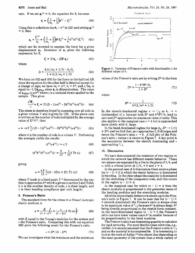
Figure 7. Variation of Poisson's ratio with functionality z for different values of k , , .

values of the Poisson's ratio are by writing D* in the form

1 - k*B*/kl, D* = 1 + B *

where

( 7 2 )

In the stretch-dominated regime u - 1 / 4 as kll - m

independent of z , because both B* and k*B*/kll tend to zero and D* approaches its maximum value of unity. This also applies to the marginal case z = 4 but is approached more slowly with kll large.

In the bend-dominated regime for large kll, D* - 1/(1 + B*) and we find that, as z approaches 2 , B diverges and hence the Poisson's ratio v - 0. A full plot of the Pois- son's ratio u versus z is shown in Figure 7. A key point is the association between the stretch dominating and u approaching l / 4 .

10. Discussion We have demonstrated the existence of two regions in

which the network has different elastic behavior. These two phases are separated by a line in the plane of l / k l l and z , with a critical point a t l/kll = 0 and z = 4.

In the general case of d dimensions there exists a phase for ( z - 1) C d in which the elastic behavior is dominated by bending. In the other phase the elasticity is dominated by the stretching of the component rods, and this occurs in the region (z - 1) > d.

In the marginal case for which ( z - 1) = d then the elastic modulus is proportional to the geometric mean of the bending modulus and the stretching modulus.

All of the above elastic behavior is shown up in the Pois- son's ratio in Figure 7. It can be seen that for ( z - 1) > 3 (stretch dominated) the Poisson's ratio is always close to its maximum value of l / 4 because k* is always large, k* being directly proportional to the stretch force constant. In the bend-dominated region ( z - 1) < 3 the Poisson's ratio can have lower values since k* is smaller because of its proportionality to the bend modulus.

The Poisson's ratio is an interesting quantity to calculate for rigid networks. For most flexible chain networks, e.g., rubber, it is usually assumed that the Poisson's ratio is ' / z and so the material is incompressible. It is interesting to look at the work of Ashby,14 who shows that depending on the exact geometry of the system then a whole variety of

1 k*(l/m* + 1/3)

B* =


different Poisson's ratios can be obtained for cellular structures whose elements deform by bending only. Also in ref 15, Morris shows that the Poisson's ratio depends on the geometry considered. In both refs 14 and 15 the results rely on the basic structure being a hexagonal arrangement of cells. For a Cayley tree we find that the Poisson's ratio varies between 0 and 0.25 and depends strongly on the values of z and k,,.

The three-dimensional results are particularly interesting since most of the networks which have been synthesized h p e functionalities of 3 or 4 since the cross- links consist of carbon atoms.

In real networks of course the actual structure is very much different from that used here for the model, and in practice the bonds can usually stretch as well as bend. For a general network structure it may be the case that the same kind of behavior is displayed as for the Cayley tree model, although the precise value of z a t which the crossover occurs may be determined by the structure considered.

ACayley tree network, however, is a useful starting point when modeling network structures and may be particularly relevant to the study of the properties of networks which


grow as "starburst" clusters. I t would be interesting to see if networks of functionality 3 and 4 can be distinguished experimentally in line with our theory.

References and Notes (1) Aharoni, S. M.; Edwards, S. F. Macromolecules 1989,22,3361. (2) Shaefer, D. W.; Keefer, K. D. Phys. Reo. Lett. 1986,56,2199. (3) Dumas, J.; Baza, S.; Serughetti, J. J. Mater. Sci. Lett. 1986,5,

478. (4) Clark, A. H.; Ross-Murphy, S. B. Adoances in Polymer Science;

Springer-Verlag: Berlin and Heidelberg, 1987; p 83. (5) Kantor, Y.; Webman, I. Phys. Reu. Lett. 1984,52, 1891. (6) Brown, W. D. Ph.D. Thesis, Physics, Cambridge, 1986. (7) Jones, J. L.; Marques, C. M. J. Phys. (Fr.) 1990,51,1113-1127. (8) Doi, M.; Kuzuu, N. Y. J . Polym. Sci., Polym. Phys. Ed. 1980,

(9) Edwards, S. F. J. Phys. (Fr.) 1988, 49, 1673. (10) Bou6, F.; Edwards, S. F.; Vilgis, T. A. J . Phys. (Fr.) 1988, 49,

(11) Thorpe, M. F.; Phillips, J. C. Solid State Commun. 1985,53,

(12) Maxwell, J. C. Trans. R. SOC. Edinburgh 1870, 26. (13) Ball, R. C.; Jones, J. L., in preparation. (14) Ashby, M. F.; Gibson, L. J. Cellular Solids, Structure and

Properties; Pergamon Press: Oxford, U.K., 1988. (15) Morris, M. I. Ph.D. Thesis, Physics, Cambridge, 1987.

18, 409-419.

1635-1645.

699 and references therein.

Documents

Elasticity of rigid networks