Electric Power Systems – Laboratory Exercise 1 Voltage ... · Electric Power Systems – Laboratory Exercise 1 Voltage and Fault Currents ... is represented by a series impedance

EIEN15 Electric Power Systems Lab 1

OS/rev4. 2016 1(20) 2016-09-16

Electric Power Systems – Laboratory Exercise 1

Voltage and Fault Currents in Power System Networks

Two different issues are studied in this laboratory exercise. First, the voltage profile over transmission and distribution lines is investigated. The attention is focused on the dependency of voltage on active and reactive power transmission as a function of the X/R ratio of a line. The impact of distributed generation and reactive compensation on the voltage profile is also investigated. Second, single-line-to-ground faults in distribution networks are investigated. Common grounding practices for distribution networks in Europe and some basic principles of ground fault protection are considered. Section I in this manual reviews the necessary theory to solve this lab exercise, Section II includes several preparatory exercises, which must be made before you come to the lab. The experimental part is described in Section III.

Section I: Theory

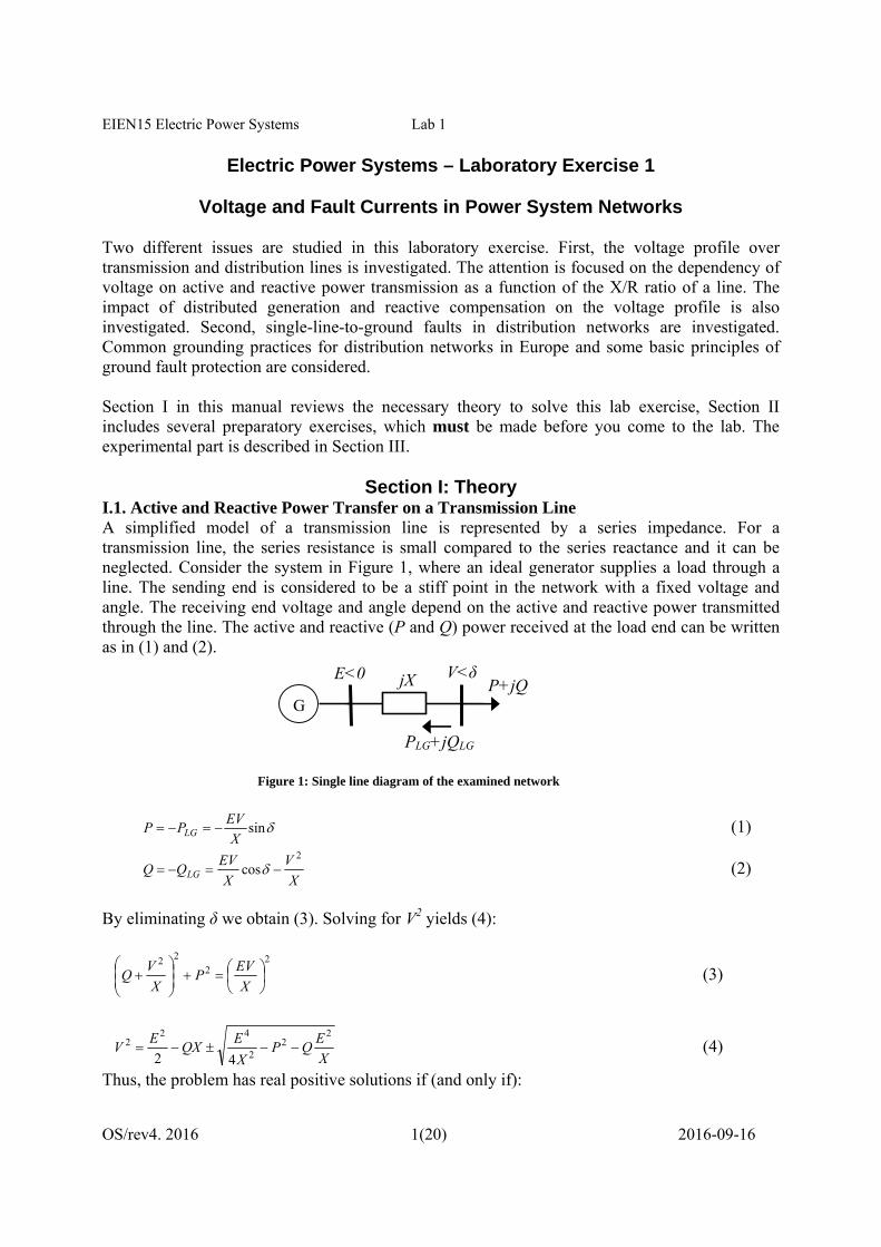
I.1. Active and Reactive Power Transfer on a Transmission Line A simplified model of a transmission line is represented by a series impedance. For a transmission line, the series resistance is small compared to the series reactance and it can be neglected. Consider the system in Figure 1, where an ideal generator supplies a load through a line. The sending end is considered to be a stiff point in the network with a fixed voltage and angle. The receiving end voltage and angle depend on the active and reactive power transmitted through the line. The active and reactive (P and Q) power received at the load end can be written as in (1) and (2).

Figure 1: Single line diagram of the examined network

sinX

EVPP LG (1)

X

V

X

EVQQ LG

2

cos (2)

By eliminating δ we obtain (3). Solving for V2 yields (4):

22

22

X

EVP

X

VQ (3)

X

EQP

X

EQX

EV

22

2

422

42 (4)

Thus, the problem has real positive solutions if (and only if):

G

E<0 V<δ jX P+jQ

PLG+jQLG


OS/rev4. 2016 2(20) 2016-09-16

2

422

4X

E

X

EQP (5)

The expression (5) can be normalized by using the short-circuit power Ssc= E2/X, and the inequality (6) is then obtained.

2

2

2

SC

SCS

QSP (6)

By setting Q = 0 in (6), we get the maximum active power that can be received at the load end:

2maxSCS

P

In a similar way, we set P = 0 in (6) and get the maximum active power, notation Pmax, that can be received at the load end. We find that

4maxSCS

Q

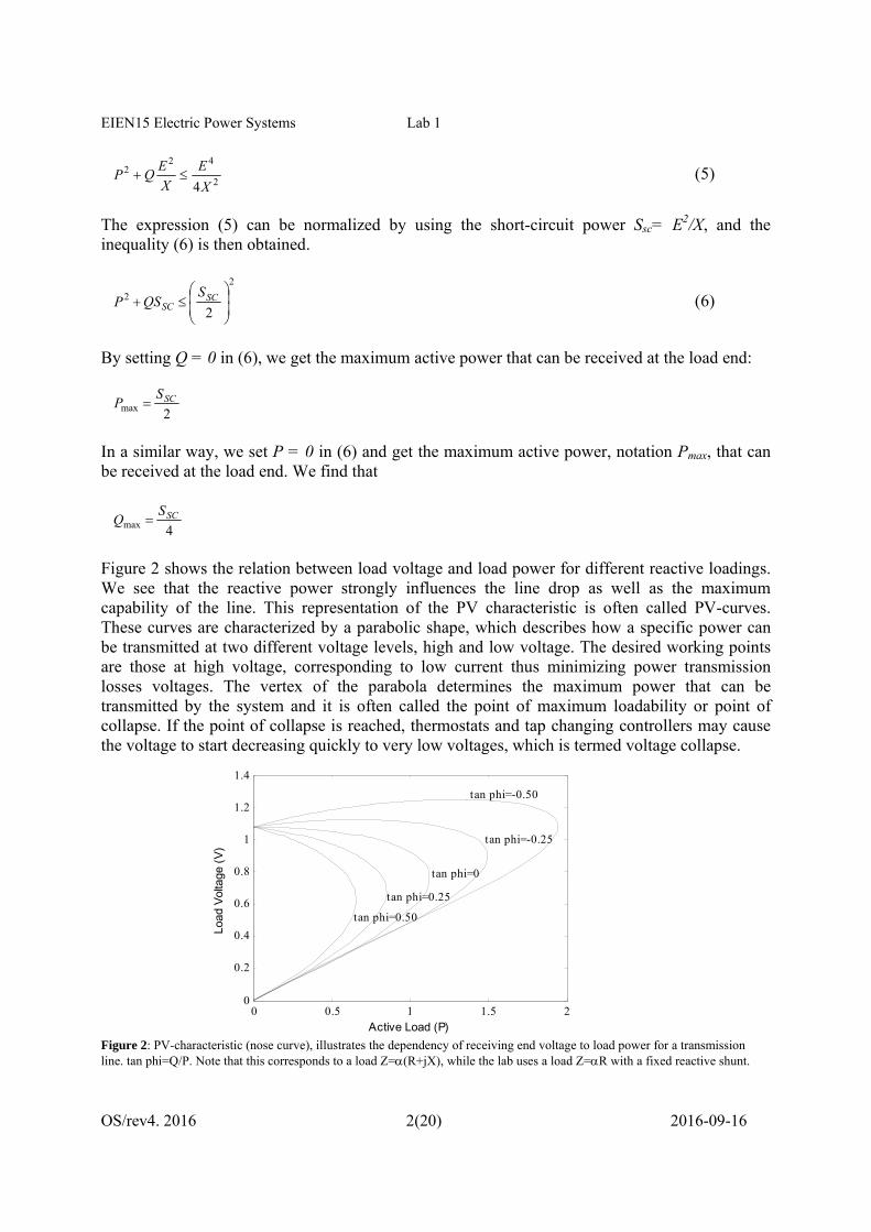
Figure 2 shows the relation between load voltage and load power for different reactive loadings. We see that the reactive power strongly influences the line drop as well as the maximum capability of the line. This representation of the PV characteristic is often called PV-curves. These curves are characterized by a parabolic shape, which describes how a specific power can be transmitted at two different voltage levels, high and low voltage. The desired working points are those at high voltage, corresponding to low current thus minimizing power transmission losses voltages. The vertex of the parabola determines the maximum power that can be transmitted by the system and it is often called the point of maximum loadability or point of collapse. If the point of collapse is reached, thermostats and tap changing controllers may cause the voltage to start decreasing quickly to very low voltages, which is termed voltage collapse.

0 0.5 1 1.5 20

0.2

0.4

0.6

0.8

1

1.2

1.4

Load

Vol

tage

(V

)

Active Load (P)

tan phi=0.50

tan phi=0.25

tan phi=0

tan phi=-0.25

tan phi=-0.50

Figure 2: PV-characteristic (nose curve), illustrates the dependency of receiving end voltage to load power for a transmission line. tan phi=Q/P. Note that this corresponds to a load Z=(R+jX), while the lab uses a load Z=R with a fixed reactive shunt.


OS/rev4. 2016 3(20) 2016-09-16

I.2. Reactive Power Compensation Consider the standard pi-link (e.g. Glover-Sarma-Overbye fig. 5.3) representation of a lossless transmission line terminated by a resistive load (R). The reactive power losses absorbed and the reactive power generated by the line are given by equations (7) and (8) respectively.

2LIQloss (7) 2CVQgen (8)

Note that Equation 8 is exactly true only if the line has a flat voltage profile, i.e. the voltage is V all along the line. This is true if generation and absorption of line reactive power are in balance:

C

L

I

VRCVLI 0

22 (9)

R=R0 is called the characteristic impedance, and the corresponding active power transported P0=V2/R0, is called natural loading or surge impedance loading (SIL). In a line operating at natural loading there is no reactive power transport whatsoever, and this is therefore its most economical operating point. In reality, power system lines are however frequently operated quite a bit above their natural loading, whereas cables (with their high capacitance) are operated below their natural loading. The purpose of reactive power compensation is to reduce the amount of reactive power transported over the lines, and thereby also reducing active losses. There are several alternatives:

Series capacitance, lowers the line series reactance and increases the natural loading; Shunt reactance, lowers the line shunt capacitance and lowers the natural loading; Shunt capacitance, increases the shunt line capacitance and increases the natural loading.

Series reactance is not used for line compensation. It is used instead to limit short-circuit currents if they are excessive. The approximate amount of shunt compensation needed to adjust the voltage at a bus is calculated from (10), the sensitivity of the bus voltage to injection of (positive or negative) reactive power: Describe the system behind the bus using a Thévenin equivalent as in Figure 1.

112

cos

X

V

X

E

V

Q

Q

V (10)

The equivalent system is unloaded and therefore δ=0 and E=V=1. Since the p.u. short-circuit capacity is SSC=1/X, the expression can be simplified:

.).(

1.).(

211

upSupX

E

X

X

V

X

E

V

Q

Q

V

SC

(11)

Increasing the voltage by 0.01 p.u, requires connecting a reactive load of –0.01·SSC p.u., i.e. a capacitor bank rated 1% of the short-circuit capacity.


OS/rev4. 2016 4(20) 2016-09-16

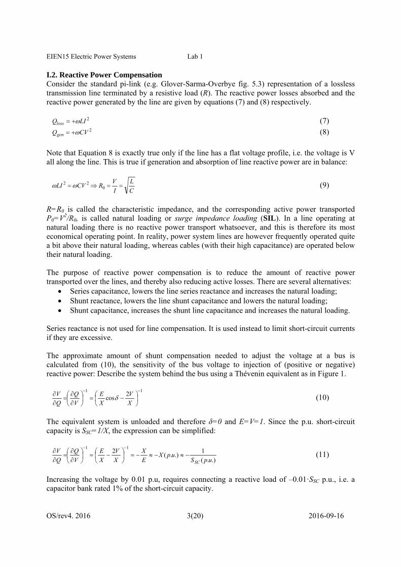
I.3. Voltage Profile in Distribution Lines In section I.1 the series resistance of the transmission line has been neglected. This is reasonable, since for a transmission line the series resistance per km is typically an order of magnitude smaller than the series inductive reactance per km. This fact no longer holds for a distribution line, for which the series resistance and the series inductive reactance are of the same order of magnitude. The series resistance must be included in the model of a distribution line, as shown in Figure 3.

Figure 3: Single line diagram of the examined network with a distribution line

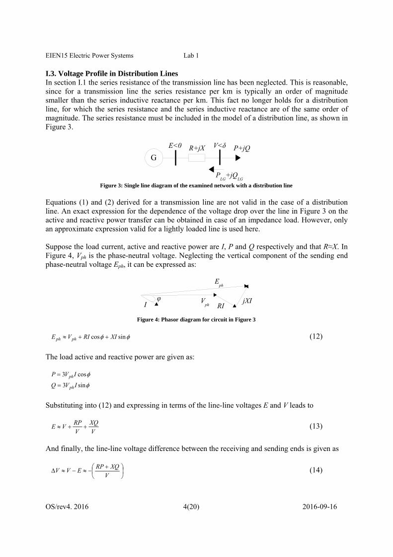
Equations (1) and (2) derived for a transmission line are not valid in the case of a distribution line. An exact expression for the dependence of the voltage drop over the line in Figure 3 on the active and reactive power transfer can be obtained in case of an impedance load. However, only an approximate expression valid for a lightly loaded line is used here. Suppose the load current, active and reactive power are I, P and Q respectively and that R≈X. In Figure 4, Vph is the phase-neutral voltage. Neglecting the vertical component of the sending end phase-neutral voltage Eph, it can be expressed as:

Figure 4: Phasor diagram for circuit in Figure 3

sincos XIRIVE phph (12)

The load active and reactive power are given as:

cos3 IVP ph sin3 IVQ ph

Substituting into (12) and expressing in terms of the line-line voltages E and V leads to

V

XQ

V

RPVE (13)

And finally, the line-line voltage difference between the receiving and sending ends is given as

V

XQRPEVV (14)


OS/rev4. 2016 5(20) 2016-09-16

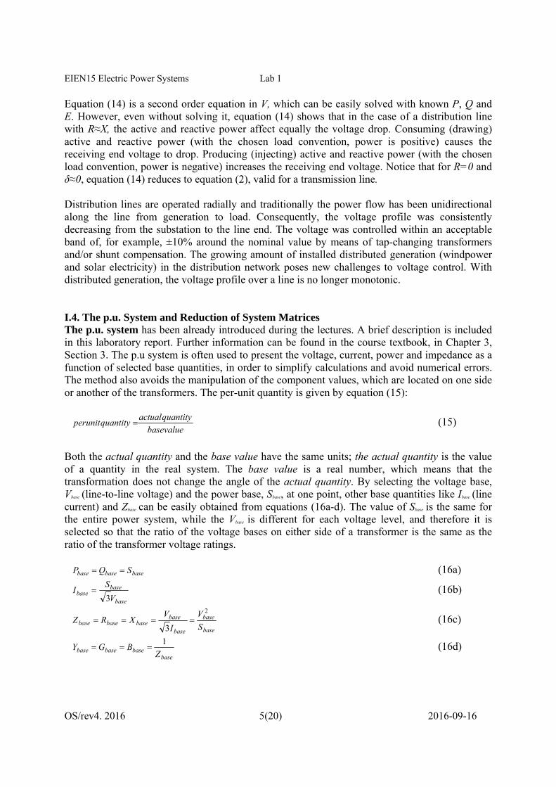
Equation (14) is a second order equation in V, which can be easily solved with known P, Q and E. However, even without solving it, equation (14) shows that in the case of a distribution line with R≈X, the active and reactive power affect equally the voltage drop. Consuming (drawing) active and reactive power (with the chosen load convention, power is positive) causes the receiving end voltage to drop. Producing (injecting) active and reactive power (with the chosen load convention, power is negative) increases the receiving end voltage. Notice that for R=0 and δ≈0, equation (14) reduces to equation (2), valid for a transmission line. Distribution lines are operated radially and traditionally the power flow has been unidirectional along the line from generation to load. Consequently, the voltage profile was consistently decreasing from the substation to the line end. The voltage was controlled within an acceptable band of, for example, ±10% around the nominal value by means of tap-changing transformers and/or shunt compensation. The growing amount of installed distributed generation (windpower and solar electricity) in the distribution network poses new challenges to voltage control. With distributed generation, the voltage profile over a line is no longer monotonic. I.4. The p.u. System and Reduction of System Matrices The p.u. system has been already introduced during the lectures. A brief description is included in this laboratory report. Further information can be found in the course textbook, in Chapter 3, Section 3. The p.u system is often used to present the voltage, current, power and impedance as a function of selected base quantities, in order to simplify calculations and avoid numerical errors. The method also avoids the manipulation of the component values, which are located on one side or another of the transformers. The per-unit quantity is given by equation (15):

valuebase

quantityactualquantityunitper (15)

Both the actual quantity and the base value have the same units; the actual quantity is the value of a quantity in the real system. The base value is a real number, which means that the transformation does not change the angle of the actual quantity. By selecting the voltage base, Vbase (line-to-line voltage) and the power base, Sbase, at one point, other base quantities like Ibase (line current) and Zbase can be easily obtained from equations (16a-d). The value of Sbase is the same for the entire power system, while the Vbase is different for each voltage level, and therefore it is selected so that the ratio of the voltage bases on either side of a transformer is the same as the ratio of the transformer voltage ratings.

basebasebase SQP (16a)

base

basebase

V

SI

3 (16b)

base

base

base

basebasebasebase S

V

I

VXRZ

2

3 (16c)

basebasebasebase Z

BGY1

(16d)


OS/rev4. 2016 6(20) 2016-09-16

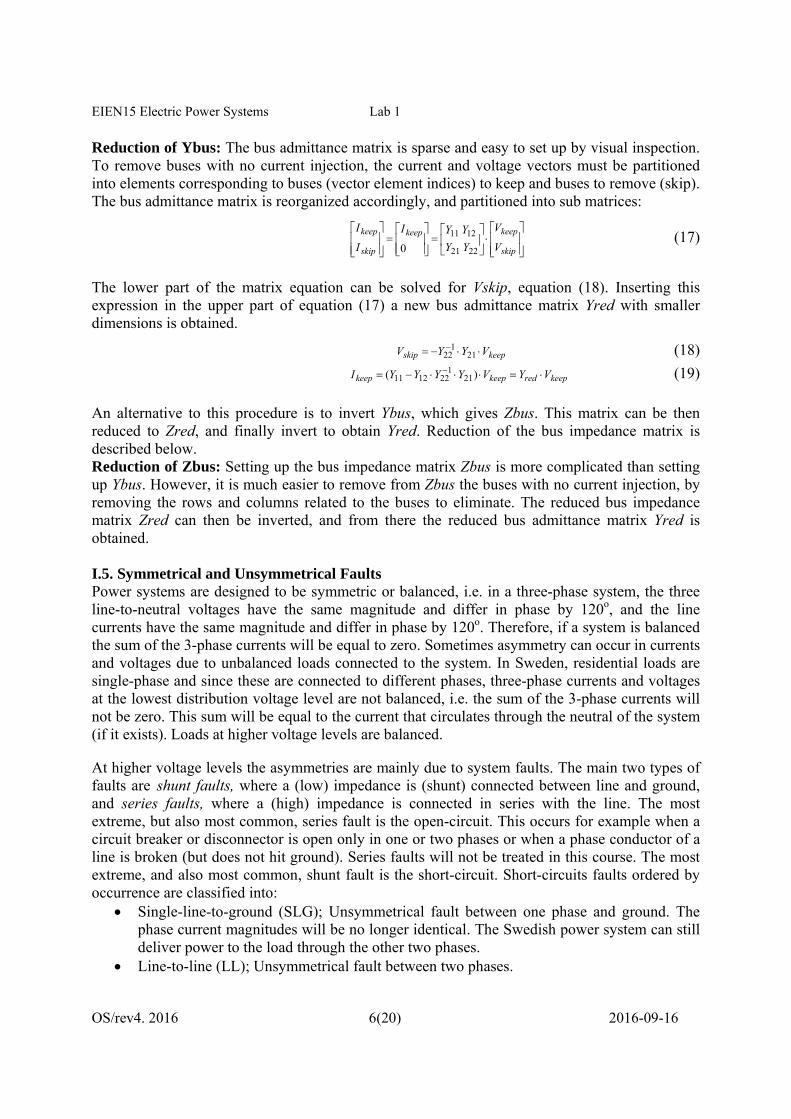
Reduction of Ybus: The bus admittance matrix is sparse and easy to set up by visual inspection. To remove buses with no current injection, the current and voltage vectors must be partitioned into elements corresponding to buses (vector element indices) to keep and buses to remove (skip). The bus admittance matrix is reorganized accordingly, and partitioned into sub matrices:

skip

keepkeep

skip

keep

V

V

YY

YYI

I

I

2221

1211

0 (17)

The lower part of the matrix equation can be solved for Vskip, equation (18). Inserting this expression in the upper part of equation (17) a new bus admittance matrix Yred with smaller dimensions is obtained.

keepskip VYYV 21

122 (18)

keepredkeepkeep VYVYYYYI )( 211

221211 (19)

An alternative to this procedure is to invert Ybus, which gives Zbus. This matrix can be then reduced to Zred, and finally invert to obtain Yred. Reduction of the bus impedance matrix is described below. Reduction of Zbus: Setting up the bus impedance matrix Zbus is more complicated than setting up Ybus. However, it is much easier to remove from Zbus the buses with no current injection, by removing the rows and columns related to the buses to eliminate. The reduced bus impedance matrix Zred can then be inverted, and from there the reduced bus admittance matrix Yred is obtained. I.5. Symmetrical and Unsymmetrical Faults Power systems are designed to be symmetric or balanced, i.e. in a three-phase system, the three line-to-neutral voltages have the same magnitude and differ in phase by 120o, and the line currents have the same magnitude and differ in phase by 120o. Therefore, if a system is balanced the sum of the 3-phase currents will be equal to zero. Sometimes asymmetry can occur in currents and voltages due to unbalanced loads connected to the system. In Sweden, residential loads are single-phase and since these are connected to different phases, three-phase currents and voltages at the lowest distribution voltage level are not balanced, i.e. the sum of the 3-phase currents will not be zero. This sum will be equal to the current that circulates through the neutral of the system (if it exists). Loads at higher voltage levels are balanced.

At higher voltage levels the asymmetries are mainly due to system faults. The main two types of faults are shunt faults, where a (low) impedance is (shunt) connected between line and ground, and series faults, where a (high) impedance is connected in series with the line. The most extreme, but also most common, series fault is the open-circuit. This occurs for example when a circuit breaker or disconnector is open only in one or two phases or when a phase conductor of a line is broken (but does not hit ground). Series faults will not be treated in this course. The most extreme, and also most common, shunt fault is the short-circuit. Short-circuits faults ordered by occurrence are classified into:

Single-line-to-ground (SLG); Unsymmetrical fault between one phase and ground. The phase current magnitudes will be no longer identical. The Swedish power system can still deliver power to the load through the other two phases.

Line-to-line (LL); Unsymmetrical fault between two phases.


OS/rev4. 2016 7(20) 2016-09-16

Double-line-to-ground or Line-to-line-to-ground (LLG); Unsymmetrical fault between two phases and ground.

Three-phase short-circuit (3Φ); It is a symmetrical fault that affects the 3-phases of the power system. The most severe short-circuit.

For all the above faults, the path of the fault current may be limited by nonzero impedance. If the impedance is equal to zero, the short-circuit is called bolted. Short- circuit faults often occur as a consequence of damage to cables and lightning strikes or trees falling on overhead lines. One of the most common reasons for three-phase short-circuit to occur is when a line or busbar is energized with grounding equipment left connected. This equipment is used for safety reasons while repairmen work on the power equipment, and it should be removed after the work is completed, and before the equipment is energized.

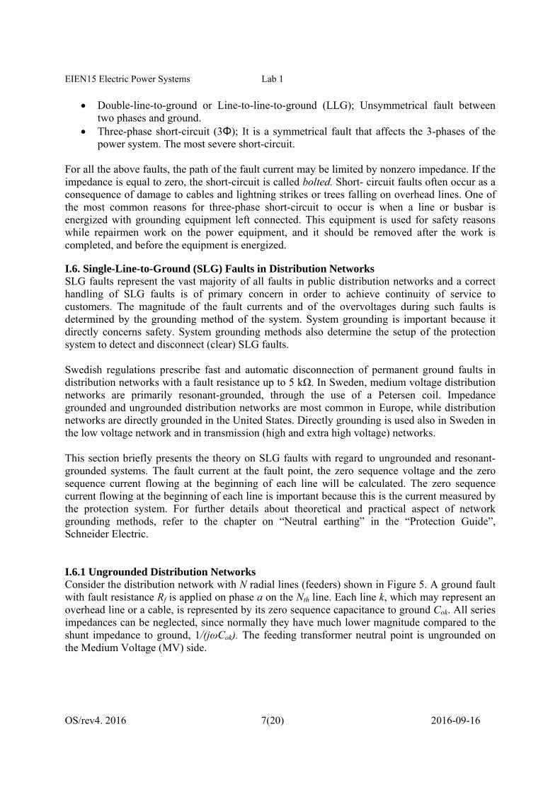
I.6. Single-Line-to-Ground (SLG) Faults in Distribution Networks SLG faults represent the vast majority of all faults in public distribution networks and a correct handling of SLG faults is of primary concern in order to achieve continuity of service to customers. The magnitude of the fault currents and of the overvoltages during such faults is determined by the grounding method of the system. System grounding is important because it directly concerns safety. System grounding methods also determine the setup of the protection system to detect and disconnect (clear) SLG faults. Swedish regulations prescribe fast and automatic disconnection of permanent ground faults in distribution networks with a fault resistance up to 5 kΩ. In Sweden, medium voltage distribution networks are primarily resonant-grounded, through the use of a Petersen coil. Impedance grounded and ungrounded distribution networks are most common in Europe, while distribution networks are directly grounded in the United States. Directly grounding is used also in Sweden in the low voltage network and in transmission (high and extra high voltage) networks. This section briefly presents the theory on SLG faults with regard to ungrounded and resonant-grounded systems. The fault current at the fault point, the zero sequence voltage and the zero sequence current flowing at the beginning of each line will be calculated. The zero sequence current flowing at the beginning of each line is important because this is the current measured by the protection system. For further details about theoretical and practical aspect of network grounding methods, refer to the chapter on “Neutral earthing” in the “Protection Guide”, Schneider Electric. I.6.1 Ungrounded Distribution Networks Consider the distribution network with N radial lines (feeders) shown in Figure 5. A ground fault with fault resistance Rf is applied on phase a on the Nth line. Each line k, which may represent an overhead line or a cable, is represented by its zero sequence capacitance to ground Cok. All series impedances can be neglected, since normally they have much lower magnitude compared to the shunt impedance to ground, 1/(jωCok). The feeding transformer neutral point is ungrounded on the Medium Voltage (MV) side.


OS/rev4. 2016 8(20) 2016-09-16

Figure 5: MV ungrounded distribution network with N lines. A SLG fault is applied on phase a of the Nth line

The SLG fault current at the fault point can be calculated using the equation in the formula sheet or by inspection of Figure 6.

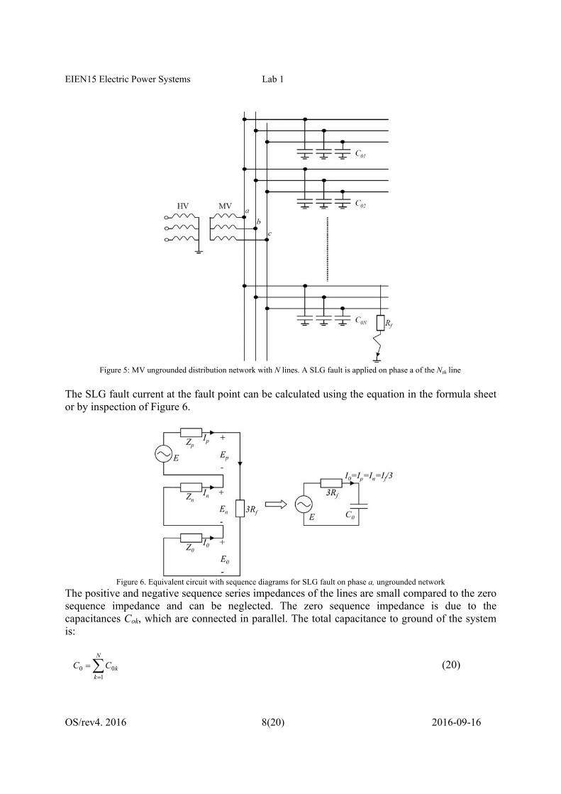
Figure 6. Equivalent circuit with sequence diagrams for SLG fault on phase a, ungrounded network

The positive and negative sequence series impedances of the lines are small compared to the zero sequence impedance and can be neglected. The zero sequence impedance is due to the capacitances Cok, which are connected in parallel. The total capacitance to ground of the system is:

N

kkCC

100 (20)


OS/rev4. 2016 9(20) 2016-09-16

Given the positive sequence phase to ground voltage E, the positive, negative and zero sequence current at the fault point are given as

ff

fnp RCj

ECj

CjR

EIIII

0

0

0

0 31133

(21)

The SLG fault current at the fault point is given as:

ff RCj

ECjI

0

0

31

3

(22)

From Figure 6, the zero sequence voltage E0 can be expressed as:

fRCj

EI

CjE

00

00 31

1

(23)

These two equations show that the fault current and the zero sequence quantities decrease with increasing fault resistance. A small amount of zero sequence voltage may exist in a distribution network also during healthy conditions because of asymmetries in the capacitances to ground. For very high fault resistance, the zero sequence quantities during a fault may be of the same order of magnitude as during healthy conditions, rendering difficult the detection of the fault. The fault current during a fault with Rf=0 is proportional to the total capacitance to ground C0. Cable lines have higher capacitance to ground per km than overhead lines. Hence, in networks with cable lines the SLG fault current has higher magnitude than in networks with only overhead lines. The zero sequence current flowing at the beginning of each healthy line is easily calculated, given the zero sequence voltage in (23):

0

000,0 31 CRj

ECjECjI

f

kkhealthyk

(24)

Because of Kirchoff’s law, the zero sequence current at the beginning of the faulted Nth line must be equal to the opposite of the sum of the zero sequence currents on all other (healthy) lines:

0

00000

1

100

1

1,0,0 31 CRj

ECCjECCjCEjII

f

NN

N

kk

N

khealthykfaultedN

(25)

By comparing equation (24) and (25), it can be seen that the zero sequence currents at the beginning of a healthy or faulted line differ in phase by 180 relative to the zero sequence voltage E0. As you will learn during the lab, this fact can be used to selectively detect and hence disconnect only the faulted line thus minimizing the number of customers experiencing a service interruption during permanent SLG faults. Also, notice that the zero sequence current flowing at the beginning of the faulted line in equation (25) differs from the zero sequence current at the fault point by the zero sequence current contribution due to the capacitance to ground of the Nth line, C0N.


OS/rev4. 2016 10(20) 2016-09-16

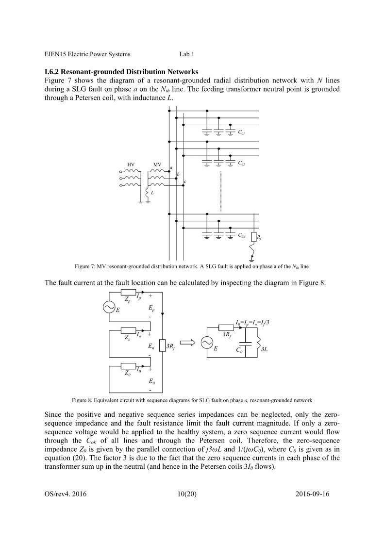
I.6.2 Resonant-grounded Distribution Networks Figure 7 shows the diagram of a resonant-grounded radial distribution network with N lines during a SLG fault on phase a on the Nth line. The feeding transformer neutral point is grounded through a Petersen coil, with inductance L.

Figure 7: MV resonant-grounded distribution network. A SLG fault is applied on phase a of the Nth line

The fault current at the fault location can be calculated by inspecting the diagram in Figure 8.

Figure 8. Equivalent circuit with sequence diagrams for SLG fault on phase a, resonant-grounded network

Since the positive and negative sequence series impedances can be neglected, only the zero-sequence impedance and the fault resistance limit the fault current magnitude. If only a zero-sequence voltage would be applied to the healthy system, a zero sequence current would flow through the Cok of all lines and through the Petersen coil. Therefore, the zero-sequence impedance Z0 is given by the parallel connection of j3ωL and 1/(jωC0), where C0 is given as in equation (20). The factor 3 is due to the fact that the zero sequence currents in each phase of the transformer sum up in the neutral (and hence in the Petersen coils 3I0 flows).


OS/rev4. 2016 11(20) 2016-09-16

The positive, negative and zero sequence current at the fault point are given as

LjRLCR

ELC

LC

LjR

E

LjCj

R

EIIII

ffff

fnp

393

31

31

333//

133 0

20

2

02

0

0

(26)

The SLG fault current at the fault point is given as:

LjRLCR

ELCI

fff

393

313

02

02

(27)

From Figure 8, the zero sequence voltage E0 can be expressed as:

LjRLCR

LEjILj

CjE

ff

393

33//

1

020

00

(28)

From the diagram in Figure 8 and inspecting equations (26) and (27), it is evident that, choosing L as L ≈ 1/(3ω2C0), the fault current at the fault location can be reduced – possibly to zero. Reducing the fault current increases the probability of self-extinguishing for temporary ground faults in overhead lines. In practice, the value of L can be adjusted to accommodate for different values of C0 due to changes in network topology. Since the value of L is chosen to compensate the total network capacitive current, it is common practice in the industry to use an “ampere” value for the Petersen coil. Notice that both the zero sequence current and voltage decrease with increasing fault resistance. It is relevant for protection relay considerations to calculate the zero-sequence current contribution of the unfaulted lines, i.e. the zero sequence current measured by the protection system on the healthy lines, and the current into the Petersen coil.

00,0 ECjI khealthyk (29)

000 3 ECjLj

EI L

(30)

In equation (30) it has been assumed that perfect compensation exists. Because of Kirchoff’s law, the zero-sequence current flowing into the faulted line (this is the zero sequence current measured by the protection system on the faulted line) must be opposite to the sum of the zero-sequence currents on the healthy lines and of the Petersen coil current divided by 3.

0000

000

1

1,0,0 3

3

3ECj

ECjECCj

III NN

LN

khealthykfaultedN

(31)

The phase relationship between the zero sequence currents flowing at the beginning of healthy and faulted lines and the zero sequence voltage does not allow in this case the discrimination of


OS/rev4. 2016 12(20) 2016-09-16

the faulted line. The zero sequence current in equations (29) and (31) are both 90 degrees ahead of the zero sequence voltage E0. Compare these results with those obtained in equation (24) and (25) for an ungrounded network. To allow for a selective detection of the faulted line, a resistor RL is normally added in parallel with the Petersen coil. The zero sequence current due to RL is in phase with the zero sequence voltage and (its opposite) flows only into the faulted line. As you will learn during the lab, with a proper choice of the resistance RL, the resistive component of the zero sequence current permits to selectively detect the faulted line in resonant-earthed networks. Figures 1 and 2 on page 10 of the Schneider “Protection Guide” help clarifying this concept.


OS/rev4. 2016 13(20) 2016-09-16

Section II: Preparatory Exercises

Matlab Exercises

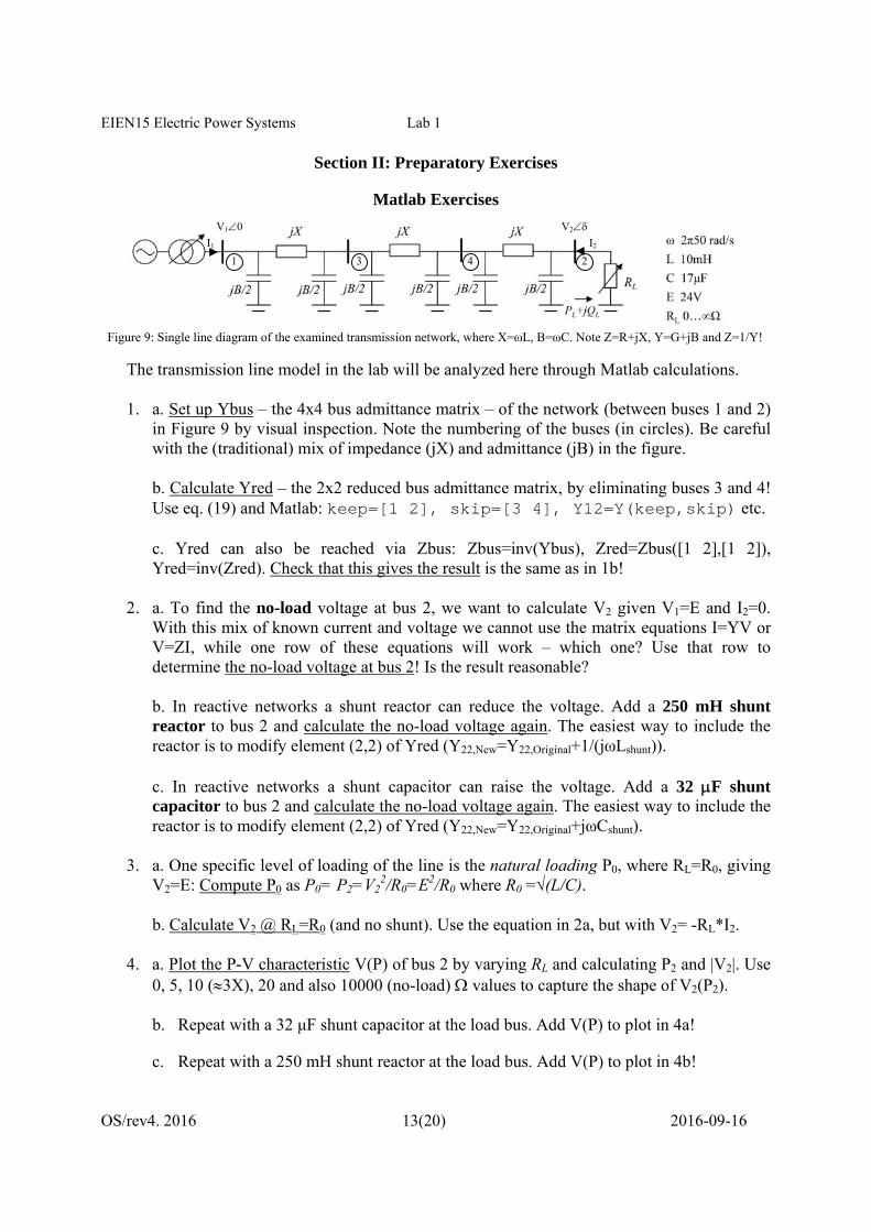
Figure 9: Single line diagram of the examined transmission network, where X=ωL, B=ωC. Note Z=R+jX, Y=G+jB and Z=1/Y!

The transmission line model in the lab will be analyzed here through Matlab calculations.

1. a. Set up Ybus – the 4x4 bus admittance matrix – of the network (between buses 1 and 2) in Figure 9 by visual inspection. Note the numbering of the buses (in circles). Be careful with the (traditional) mix of impedance (jX) and admittance (jB) in the figure.

b. Calculate Yred – the 2x2 reduced bus admittance matrix, by eliminating buses 3 and 4! Use eq. (19) and Matlab: keep=[1 2], skip=[3 4], Y12=Y(keep,skip) etc.

c. Yred can also be reached via Zbus: Zbus=inv(Ybus), Zred=Zbus([1 2],[1 2]), Yred=inv(Zred). Check that this gives the result is the same as in 1b!

2. a. To find the no-load voltage at bus 2, we want to calculate V2 given V1=E and I2=0. With this mix of known current and voltage we cannot use the matrix equations I=YV or V=ZI, while one row of these equations will work – which one? Use that row to determine the no-load voltage at bus 2! Is the result reasonable?

b. In reactive networks a shunt reactor can reduce the voltage. Add a 250 mH shunt reactor to bus 2 and calculate the no-load voltage again. The easiest way to include the reactor is to modify element (2,2) of Yred (Y22,New=Y22,Original+1/(jωLshunt)).

c. In reactive networks a shunt capacitor can raise the voltage. Add a 32 F shunt capacitor to bus 2 and calculate the no-load voltage again. The easiest way to include the reactor is to modify element (2,2) of Yred (Y22,New=Y22,Original+jωCshunt).

3. a. One specific level of loading of the line is the natural loading P0, where RL=R0, giving V2=E: Compute P0 as P0= P2=V2

2/R0=E2/R0 where R0 =√(L/C).

b. Calculate V2 @ RL=R0 (and no shunt). Use the equation in 2a, but with V2= -RL*I2.

4. a. Plot the P-V characteristic V(P) of bus 2 by varying RL and calculating P2 and |V2|. Use 0, 5, 10 (3X), 20 and also 10000 (no-load) values to capture the shape of V2(P2).

b. Repeat with a 32 μF shunt capacitor at the load bus. Add V(P) to plot in 4a!

c. Repeat with a 250 mH shunt reactor at the load bus. Add V(P) to plot in 4b!

1 3 4 2

V10 V2

I2 I1


OS/rev4. 2016 14(20) 2016-09-16

PowerWorld Exercises

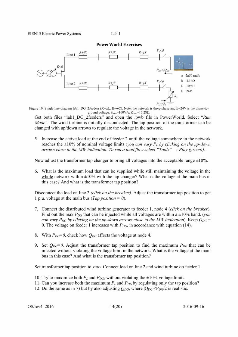
Figure 10: Single line diagram lab1_DG_2feeders (X=ωL, B=ωC). Note: the network is three-phase and E=24V is the phase-to-

ground voltage. Sbase=100VA. Zbase=17.28Ω.

Get both files “lab1_DG_2feeders” and open the .pwb file in PowerWorld. Select “Run Mode”. The wind turbine is initially disconnected. The tap position of the transformer can be changed with up/down arrows to regulate the voltage in the network.

5. Increase the active load at the end of feeder 2 until the voltage somewhere in the network reaches the ±10% of nominal voltage limits (you can vary PL by clicking on the up-down arrows close to the MW indication. To run a load flow select “Tools” → Play (green)).

Now adjust the transformer tap changer to bring all voltages into the acceptable range ±10%.

6. What is the maximum load that can be supplied while still maintaining the voltage in the whole network within ±10% with the tap changer? What is the voltage at the main bus in this case? And what is the transformer tap position?

Disconnect the load on line 2 (click on the breaker). Adjust the transformer tap position to get 1 p.u. voltage at the main bus (Tap position = 0).

7. Connect the distributed wind turbine generator to feeder 1, node 4 (click on the breaker). Find out the max PDG that can be injected while all voltages are within a ±10% band. (you can vary PDG by clicking on the up-down arrows close to the MW indication). Keep QDG = 0. The voltage on feeder 1 increases with PDG, in accordance with equation (14).

8. With PDG=0, check how QDG affects the voltage at node 4.

9. Set QDG=0. Adjust the transformer tap position to find the maximum PDG that can be injected without violating the voltage limit in the network. What is the voltage at the main bus in this case? And what is the transformer tap position?

Set transformer tap position to zero. Connect load on line 2 and wind turbine on feeder 1.

10. Try to maximize both PL and PDG, without violating the ±10% voltage limits. 11. Can you increase both the maximum PL and PDG by regulating only the tap position? 12. Do the same as in 7) but by also adjusting QDG, where |QDG|<PDG/2 is realistic.


OS/rev4. 2016 15(20) 2016-09-16

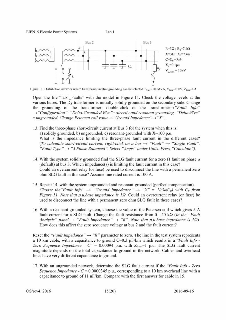
Figure 11: Distribution network where transformer neutral grounding can be selected. Sbase=100MVA, Vbase=10kV, Zbase=1Ω

Open the file “lab1_Faults” with the model in Figure 11. Check the voltage levels at the various buses. The Dy transformer is initially solidly grounded on the secondary side. Change the grounding of the transformer: double-click on the transformer→“Fault Info” →“Configuration”. “Delta-Grounded Wye”=directly and resonant grounding. “Delta-Wye” =ungrounded. Change Petersen coil value→“Ground Impedance”→“X”.

13. Find the three-phase short-circuit current at Bus 3 for the system when this is: a) solidly grounded, b) ungrounded, c) resonant-grounded with X=100 p.u. What is the impedance limiting the three-phase fault current in the different cases? (To calculate short-circuit current, right-click on a bus → “Fault” → “Single Fault”. “Fault Type” → “3 Phase Balanced”. Select “Amps” under Units. Press “Calculate”).

14. With the system solidly grounded find the SLG fault current for a zero fault on phase a (default) at bus 3. Which impedance(s) is limiting the fault current in this case? Could an overcurrent relay (or fuse) be used to disconnect the line with a permanent zero ohm SLG fault in this case? Assume line rated current is 100 A.

15. Repeat 14. with the system ungrounded and resonant-grounded (perfect compensation). Choose the“Fault Info” → “Ground Impedance” → “X” = 1/(3ωC0) with C0 from Figure 11. Note that p.u.base impedance is 1Ω. Could an overcurrent relay (or fuse) be used to disconnect the line with a permanent zero ohm SLG fault in these cases?

16. With a resonant-grounded system, choose the value of the Petersen coil which gives 5 A fault current for a SLG fault. Change the fault resistance from 0…20 kΩ (In the “Fault Analysis” panel → “Fault Impedance” → “R”. Note that p.u.base impedance is 1Ω). How does this affect the zero sequence voltage at bus 2 and the fault current?

Reset the “Fault Impedance” → “R” parameter to zero. The line in the test system represents a 10 km cable, with a capacitance to ground C=0.3 μF/km which results in a “Fault Info - Zero Sequence Impedance - C” = 0.00094 p.u. with Zbase=1 p.u. The SLG fault current magnitude depends on the total capacitance to ground in the network. Cables and overhead lines have very different capacitance to ground.

17. With an ungrounded network, determine the SLG fault current if the “Fault Info - Zero Sequence Impedance - C = 0.0000345 p.u., corresponding to a 10 km overhead line with a capacitance to ground of 11 nF/km. Compare with the first answer for cable in 15.

3F


OS/rev4. 2016 16(20) 2016-09-16

Section III: Experiments

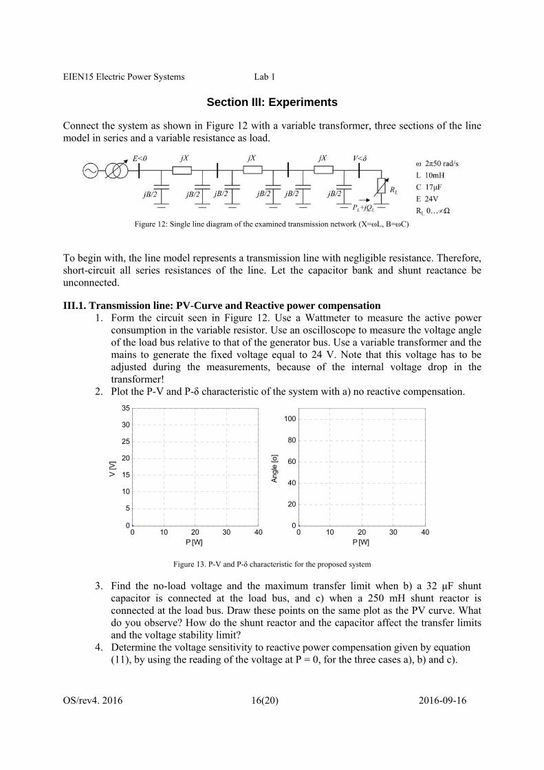
Connect the system as shown in Figure 12 with a variable transformer, three sections of the line model in series and a variable resistance as load.

Figure 12: Single line diagram of the examined transmission network (X=ωL, B=ωC)

To begin with, the line model represents a transmission line with negligible resistance. Therefore, short-circuit all series resistances of the line. Let the capacitor bank and shunt reactance be unconnected.

III.1. Transmission line: PV-Curve and Reactive power compensation 1. Form the circuit seen in Figure 12. Use a Wattmeter to measure the active power

consumption in the variable resistor. Use an oscilloscope to measure the voltage angle of the load bus relative to that of the generator bus. Use a variable transformer and the mains to generate the fixed voltage equal to 24 V. Note that this voltage has to be adjusted during the measurements, because of the internal voltage drop in the transformer!

2. Plot the P-V and P-δ characteristic of the system with a) no reactive compensation.

0 10 20 30 400

5

10

15

20

25

30

35

P [W]

V [V

]

0 10 20 30 400

20

40

60

80

100

P [W]

Ang

le [o

]

Figure 13. P-V and P-δ characteristic for the proposed system

3. Find the no-load voltage and the maximum transfer limit when b) a 32 μF shunt capacitor is connected at the load bus, and c) when a 250 mH shunt reactor is connected at the load bus. Draw these points on the same plot as the PV curve. What do you observe? How do the shunt reactor and the capacitor affect the transfer limits and the voltage stability limit?

4. Determine the voltage sensitivity to reactive power compensation given by equation (11), by using the reading of the voltage at P = 0, for the three cases a), b) and c).


OS/rev4. 2016 17(20) 2016-09-16

Compare the results to those obtained by using the rule of thumb V /Q 1/ SSC(p.u.)

V

Q

Vcomp Vuncomp

Qcomp

5. Use the measured PV-characteristic for the uncompensated system to determine the natural loading of the line. Compare it with the calculated value.

6. Plot the voltage as a function of the position on the line, when the line is loaded below, at and above its natural loading.

III.2. Short-circuit impedance and power Make a short circuit test on the load bus as follows (disconnect any shunt compensation). Determine the short-circuit-power Ssc by measuring the no-load voltage and the short-circuit current and multiply the two. The short-circuit impedance is found by dividing the no-load voltage with the short-circuit-current. III.3. Voltage Profile on Distribution Lines Disconnect the voltage supply and connect the second line model (also three sections) in parallel with the first model, as shown in Figure 10. The line models should now represent distribution overhead lines with an X/R ratio of approximately one. Hence, insert the series resistances of the π-model in series with the inductive reactances. For short distribution overhead lines, the shunt capacitance can be neglected. Hence, disconnect the capacitances of the π-model from the circuit. In the lab set-up, the distributed generation is not a wind turbine. Instead, a battery in series with a resistor Rinv (which may represent a solar PV panel) can be connected to the line through an inverter which implements a Maximum Power Point tracking (MPPT) algorithm. The power delivered from the battery to the grid can be varied by varying the resistor Rinv.

Use a variable transformer and the mains to generate a fixed voltage equal to 50 V. Connect a variable load resistor at the end of one line and use a Wattmeter to measure the active power consumption. Do not connect the inverter yet. In the following, always keep the voltage in the whole network within ±10% of nominal voltage.

7. What is the maximum power that can be delivered to the load resistor if the voltage at the variable transformer bus is regulated to nominal? What are the voltages at all nodes of the two line models in this case? Draw the voltage profile at all nodes.

8. Can the maximum power delivered to the load be increased without violating the voltage limits by acting on the variable transformer?

Regulate the variable transformer to get 50V at the transformer bus and maximum power delivered to the load. Connect the battery with the inverter at the end of the second line model to study the impact of distributed generation on the voltage profile.

9. Vary the delivered active power from the inverter by means of the variable resistor Rinv. How is this affecting the voltage profile on the second line?

10. While adjusting the voltage at the transformer bus to 50V, find the maximum active power that can be delivered by the inverter without violating the voltage limit. Draw the voltage profile at all nodes.


OS/rev4. 2016 18(20) 2016-09-16

Keep the inverter power fixed. Acting only on the variable transformer, it is not possible to increase the power delivered to the load without violating the voltage limit in the network. Try!

11. Suggest how the maximum power delivered to the load could be increased without violating the voltage limit of ±10%. Try your proposal!

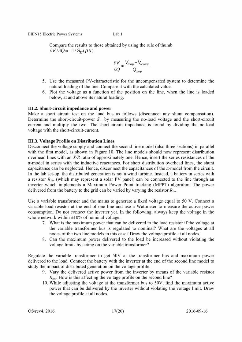
III.4. Grounding in Distribution Networks The model of the distribution network used in this lab exercise is shown in Fig 13. You will either work with a model representing two cables or with a model representing two overhead lines. To begin with, you will investigate the fault current in an ungrounded system.

Figure 13: Distribution network model used in the lab.

III.4.1 Ungrounded Distribution Network Be sure that the neutral point at the secondary side of the distribution transformer is ungrounded. Connect the three-phase transformer to the mains and set the voltage to 30V.

1. Inspect voltages and currents on the LabView measuring panel. Is there any zero-sequence voltage or current in the system?

2. On the LabView measuring panel, check the value of the potential difference between the neutral point of the transformer and reference ground (VnG).

3. Apply a solid SLG fault (phase a to ground) at the end of feeder 1. Inspect the following quantities on the measuring panel and report their complex value (magnitude and angle):

I0,feeder 1 I0,feeder 2

Ia,feeder 1 = If V0 VaG VbG VcG

4. What happens to the line-ground voltage on the two unfaulted phases? Can you

explain with reference to the diagram for a three-phase symmetrical voltage system? What is a requirement for the isolation in ungrounded networks?


OS/rev4. 2016 19(20) 2016-09-16

5. With the SLG fault applied, check again the value of the potential difference between the transformer neutral point and the reference ground (VnG) on the LabView measuring panel. This is the zero sequence voltage!

6. You have seen that the zero-sequence quantities were all zero before the fault. Can the zero-sequence voltage V0 be used for protection to detect a SLG fault? What is the major disadvantage of using only V0 for fault detection?

In case of a permanent SLG fault in real distribution systems, it is important to selectively disconnect only the faulted feeder and to continue to deliver power to the customers connected on the unfaulted part of the system.

7. What is the phase relationship between V0 and I0 in the unfaulted and in the faulted feeder respectively? Propose a principle on which a selective protection system could be based. Take help also from equations (24) and (25).

8. What happens to V0 and I0 if the SLG fault is applied through a fault resistor, when the value of the resistance is increased?

III.4.2 Resonant-grounded Distribution Network Disconnect any fault, bring the voltage down to 0V and disconnect the mains. Connect a variable inductor between the neutral of the distribution transformer secondary side and the reference ground. The distribution network is now resonant-grounded. Reconnect the mains and set the voltage to 30V.

9. Apply a solid SLG fault on phase a of feeder 2. Tune the inductor to match the total capacitance to ground C0,Tot. How can you know when the system is perfectly tuned?

10. What is the value of L in this case? Why the fault current is not zero even though the system is perfectly compensated?

Ideally, with no resistive losses and in case of perfect compensation, the current magnitude at the fault location would be equal to zero. However, the zero-sequence currents at the beginning of each feeder and from the Petersen coil would not be zero.

11. Inspect the following quantities on the measuring panel and report their complex value (magnitude and angle):

I0,feeder 1 I0,feedere 2 InG = IL


12. What are the voltages on the unfaulted phases and the zero sequence voltage V0? What

is the relation between I0,feeder_1, I0,feeder_2 and IL (= InG)? Perfect tuning of the system is difficult to achieve during all conditions. Mistuning may arise because of topological changes in the network, for ex. because one line is taken out of service.


OS/rev4. 2016 20(20) 2016-09-16

This changes the total capacitance to ground in the network. You will study the effect of mistuning by changing the value of the coil inductance with both lines connected.

13. Change the value of the variable coil inductance and observe how this affects the fault current If and the zero sequence voltage V0

14. Vary the coil inductance so to perfectly compensate the system zero sequence capacitance. What is the relationship between V0, and I0,feeder_1, I0,feeder_2 respectively? Could a protection system based on the phase relationship between these quantities selectively detect the faulted line?

Keep the system perfectly tuned. Disconnect the SLG fault. Bring the voltage down to 0V and disconnect the mains. Insert a resistor RL in parallel with the Petersen coil. Reconnect the mains and set the voltage to 30V.

15. Apply a SLG fault on feeder 1. Inspect the following quantities on the measuring panel and report their complex value (magnitude and angle):

I0,feeder 1 I0,feeder 2 InG = IL


16. What is the major difference compared with the case without resistor RL? What is the

advantage with the resistor RL concerning selective fault detection?

Documents

Electric Power Systems – Laboratory Exercise 1 Voltage ... · Electric Power Systems – Laboratory Exercise 1 Voltage and Fault Currents ... is represented by a series impedance