0-1

Electromagnetic Fields and Waves

Reference: OLVER A.D.

Microwave and Optical Transmission John Wiley & Sons, 1992, 1997

Shelf Mark: NV 135 Tim Coombs – tac1000@cam.ac.uk, 2003 WebSite: www2.eng.cam.ac.uk/~tac1000/emfieldsandwaves.htm

0-2

This course is concerned with transmission, either of electromagnetic wave along a cable (i.e. a transmission line), or, an electromagnetic wave through the ‘ether’. During the first half of these lectures we will develop the differential equations which describe the propagation of a wave along a transmission line. Then we will use these equations to demonstrate that these waves exhibit reflection and have impedance and above all transmit power. During the second half of these lectures we will look at the behaviour of waves in free space and in particular different types of antennae for transmission and reception of electromagnetic waves.

0. Introduction

An ideal transmission line is defined to be a link between two points in which the signal at any point equals the initiating signal. I.e. that transmission takes place instantaneously and that there is no attenuation. Real world transmission lines are not ideal, there is attenuation and there are delays in transmission Notation :

x means x is complex

j xxe β is short-hand for ( )Re j x txe β ω+

which equals -- cosx t x xω β+ + ∠

0-3

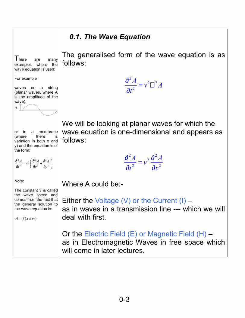
There are many examples where the wave equation is used: For example waves on a string (planar waves, where A is the amplitude of the wave),

or in a membrane (where there is variation in both x and y) and the equation is of the form:

2 2 22

2 2 2

A A Avt x y

∂ ∂ ∂= + ∂ ∂ ∂

Note: The constant v is called the wave speed and comes from the fact that the general solution to the wave equation is:

( )A f x vt= ±

0.1. The Wave Equation The generalised form of the wave equation is as follows:

22 2

2

A v At

∂ = ∇∂

We will be looking at planar waves for which the wave equation is one-dimensional and appears as follows:

2 22

2 2

A Avt x

∂ ∂=∂ ∂

Where A could be:- Either the Voltage (V) or the Current (I) – as in waves in a transmission line --- which we will deal with first. Or the Electric Field (E) or Magnetic Field (H) – as in Electromagnetic Waves in free space which will come in later lectures.

A

0-4

0. Introduction............................................................................. 0-2

0.1. The Wave Equation......................................................... 0-3

1. Electrical Waves – Olver pp 269-272 ..................................... 1-1

1.1. Telegrapher’s Equations ...................................................... 1-1

1.2. Travelling Wave Equations.............................................. 1-2

1.3. Lossy Transmission Lines ............................................... 1-3

1.4. Wave velocity -- v ............................................................ 1-6

1.5. Sample Calculation- wave length .................................... 1-7

1.6. When is AC – DC ? ......................................................... 1-8

1.7. Example – When Is Wave Theory relevant? ................... 1-9

2. Characteristic Impedance Olver – pp 269-272 ...................... 2-2

2.1. Derivation ........................................................................ 2-2

2.2. Summarizing ................................................................... 2-3

2.3. Characteristic Impedance – Example 1........................... 2-4

2.4. Characteristic Impedance – Example 2........................... 2-4

3. Reflection – Olver pp273-274................................................. 3-1

3.1. Voltage reflection coefficient............................................ 3-1

3.2. Power Reflection ............................................................. 3-2

3.3. Standing Waves .............................................................. 3-3

3.4. Summarizing ................................................................... 3-4

3.5. Example - Termination (e.g. of BNC lines) ...................... 3-5

3.6. Example - Ringing........................................................... 3-8

3.7. ¼ Wave Matching.......................................................... 3-10

3.7.1. Example - Quarter Wave transformer....................... 3-12

4. Electromagnetic Fields ........................................................... 4-1

4.1. Definitions ....................................................................... 4-1

4.2. The Laws of Electromagnetism ....................................... 4-4

4.2.1. Maxwell’s Laws........................................................... 4-4

4.2.2. Gauss’s Laws ............................................................. 4-5

5. Electromagnetic Waves.......................................................... 5-1

0-5

5.1. Derivation of Wave Equation........................................... 5-1

5.2. Intrinsic Impedance ......................................................... 5-4

6. Reflection and refraction of waves ......................................... 6-1

6.1. Reflection of Incident wave normal to the plane of the reflection .................................................................................... 6-1

6.2. Reflection from a dielectric boundary of wave at oblique incidence.................................................................................... 6-2

6.2.1. Snell’s Law of refraction ............................................. 6-3

6.2.2. Incident and Reflected Power..................................... 6-4

6.2.3. Perpendicularly polarised waves ................................ 6-5

6.2.4. Parallel Polarised Waves............................................ 6-6

6.2.5. Comparison between reflections of parallel and perpendicularly polarised waves ............................................ 6-7

6.3. Total Internal Reflection........................................................ 6-8

6.4. Comparison of Transmission Line & Free Space Waves. 6-9

6.5. Example – Characteristic Impedance............................ 6-10

6.6. Example – Electromagnetic Waves................................6-11

7. Antennae................................................................................ 7-1

7.1. Slot and aperture antennae............................................. 7-1

7.1.1. Horn Antennae............................................................ 7-2

7.1.2. Laser .......................................................................... 7-2

7.2. Dipole Antennae.............................................................. 7-3

7.2.1. Half-Wave Dipole........................................................ 7-3

7.2.2. Short Dipole................................................................ 7-3

7.2.3. Half Dipole.................................................................. 7-4

7.3. Loop Antennae ................................................................ 7-4

7.4. Reflector Antennae.......................................................... 7-5

7.5. Array antennae................................................................ 7-6

7.6. The Poynting Vector ........................................................ 7-7

7.6.1. Example – Duck a la microwave................................. 7-9

8. Radio...................................................................................... 8-1

0-6

8.1. Radiation Resistance ...................................................... 8-1

8.2. Gain................................................................................. 8-1

8.3. Effective Area .................................................................. 8-2

8.4. Example – Power Transmission ...................................... 8-3

1-1

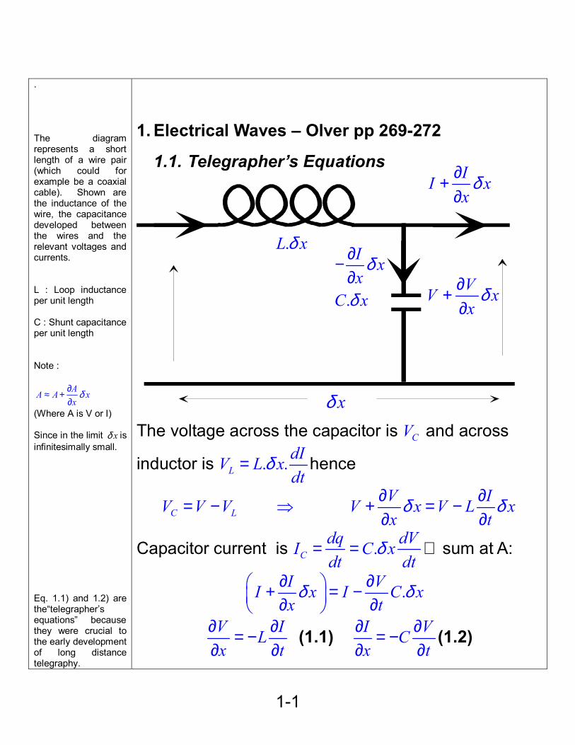
. The diagram represents a short length of a wire pair (which could for example be a coaxial cable). Shown are the inductance of the wire, the capacitance developed between the wires and the relevant voltages and currents. L : Loop inductance per unit length C : Shunt capacitance per unit length Note :

AA A xx

δ∂≈ +∂

(Where A is V or I) Since in the limit xδ is infinitesimally small. Eq. 1.1) and 1.2) are the“telegrapher’s equations” because they were crucial to the early development of long distance telegraphy.

1. Electrical Waves – Olver pp 269-272

1.1. Telegrapher’s Equations

The voltage across the capacitor is CV and across

inductor is . .LdIV L xdt

δ= hence

C LV IV V V V x V L xx t

δ δ∂ ∂= − ⇒ + = −∂ ∂

Capacitor current is .Cdq dVI C xdt dt

δ= = ∴ sum at A:

.I VI x I C xx t

δ δ∂ ∂ + = − ∂ ∂

V ILx t

∂ ∂= −∂ ∂

(1.1) I VCx t

∂ ∂= −∂ ∂

(1.2)

VV xx

δ∂+∂

II xx

δ∂+∂

.C xδ

.L xδ I xx

δ∂−∂

xδ

1-2

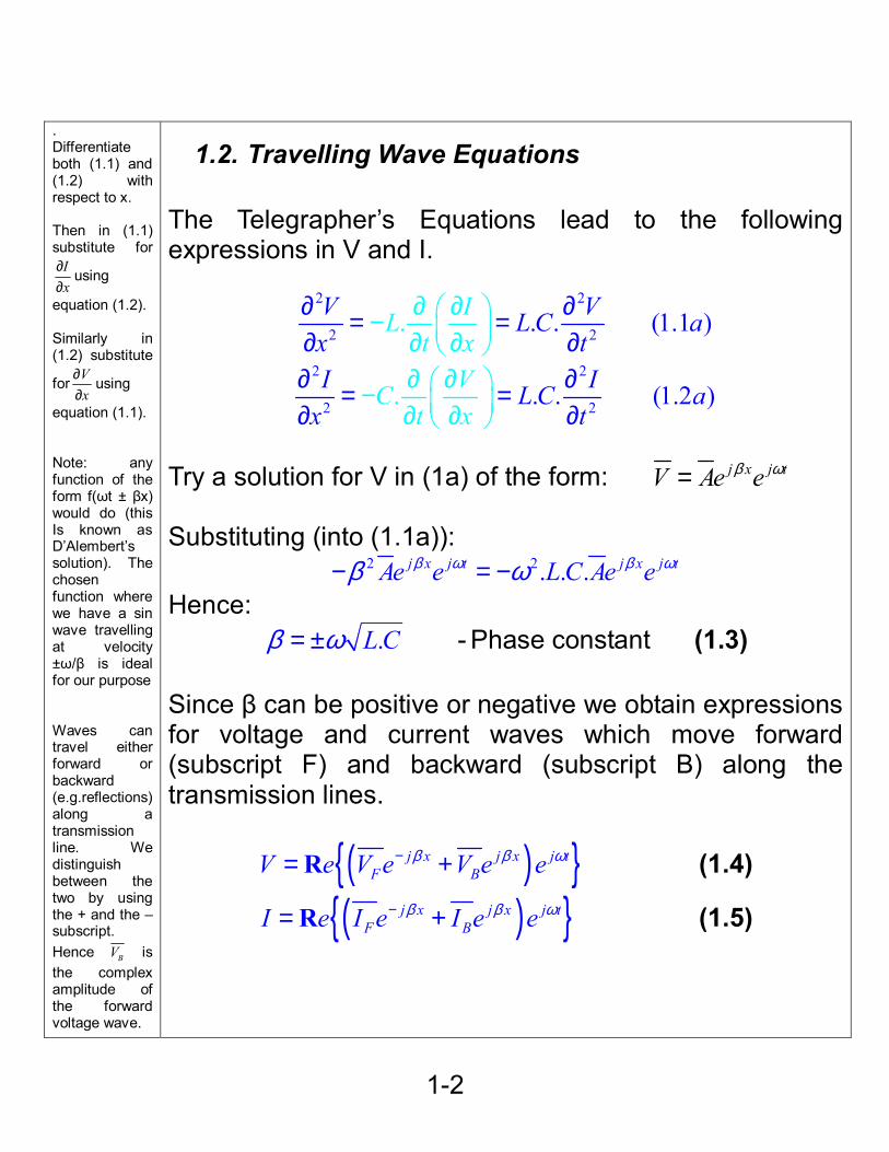
. Differentiate both (1.1) and (1.2) with respect to x. Then in (1.1) substitute for Ix

∂∂

using

equation (1.2). Similarly in (1.2) substitute

for Vx

∂∂

using

equation (1.1). Note: any function of the form f(ωt ± βx) would do (this Is known as D’Alembert’s solution). The chosen function where we have a sin wave travelling at velocity ±ω/β is ideal for our purpose Waves can travel either forward or backward (e.g.reflections) along a transmission line. We distinguish between the two by using the + and the – subscript. Hence BV is the complex amplitude of the forward voltage wave.

1.2. Travelling Wave Equations The Telegrapher’s Equations lead to the following expressions in V and I.

2 2

2 2. . (1.1. )ILt

V VLC atxx

∂ ∂ − ∂ ∂∂ =

∂∂=

∂

2 2

2 2. . (1.2. )VCt

I ILC atxx

∂ ∂ − ∂ ∂∂ =

∂∂=

∂

Try a solution for V in (1a) of the form: j x j tV Ae eβ ω= Substituting (into (1.1a)):

2 2. . .j x j t j x j tAe e LC Ae eβ ω β ωβ ω− = − Hence:

.LCβ ω= ± - Phase constant (1.3) Since β can be positive or negative we obtain expressions for voltage and current waves which move forward (subscript F) and backward (subscript B) along the transmission lines.

( ) j x j x j tF BV e V e V e eβ β ω−= +R (1.4)

( ) j x j x j tF BI e I e I e eβ β ω−= +R (1.5)

1-3

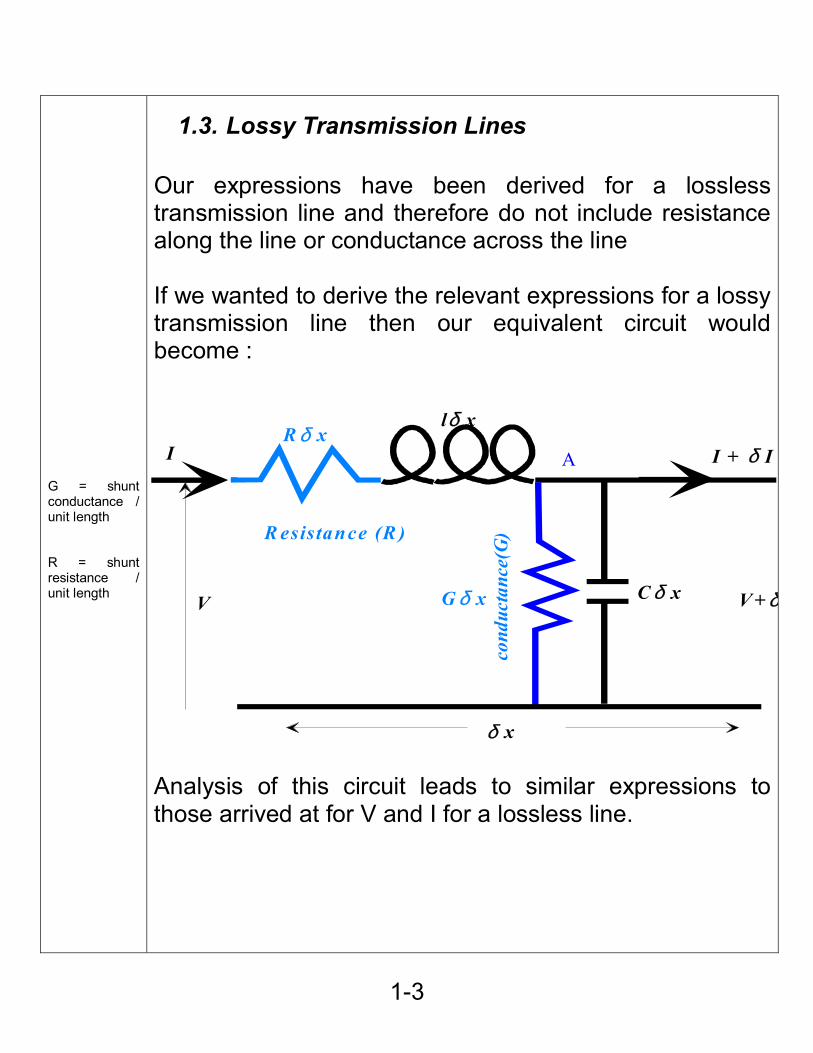
G = shunt conductance / unit length R = shunt resistance / unit length

1.3. Lossy Transmission Lines Our expressions have been derived for a lossless transmission line and therefore do not include resistance along the line or conductance across the line If we wanted to derive the relevant expressions for a lossy transmission line then our equivalent circuit would become :

R esistance (R )co

nduc

tanc

e(G

)

I I + δ I

V V + δ

R δ xlδ x

G δ x C δ x

δ x

A

Analysis of this circuit leads to similar expressions to those arrived at for V and I for a lossless line.

1-4

For simplicity we assume that V and I have a time dependence of

j te ω. (As has

already been demonstrated for lossless lines.) i.e.

( )j tI f e ω=then

dI j Idt

ω=

Using Kirchoff’s voltage law to sum voltages and ignoring second order terms such as δzδI we get:

( ) 0V R xI j L xI V Vδ ω δ δ− − − + =

i.e. ( )V R j L Ix

δ ωδ

= − + & in the limit :

( )V R j L Ix

ω∂ = − +∂

c.f. V IL j LIx t

ω∂ ∂= − = −∂ ∂

(1.1)

Similarly using Kirchoff’s current law to sum currents will give us:

( ) 0I G xV j C xV I Iδ ω δ δ− − − + =

i.e. ( )I G j C Vx

δ ωδ

= − + & in the limit :

( )I G j C Vx

ω∂ = − +∂

c.f. I VC j CVx t

ω∂ ∂= − = −∂ ∂

(1.2)

1-5

So now our expressions for voltage and current gain an extra term

( ) ( )( ) ( . . 1.4)j x j x j tF BV e V e V e e c fβ β ωα α− + += +R

( ) ( )( ) ( . . 1.5)j x j x j tF BI e I e I e e c fβαβ ωα + +−= +R

We therefore define a new term the propagation constant

jγ α β= + Where the phase constant

.LCβ ω= ± as before and the real term corresponds to the attenuation along the line and is known as the attenuation constant At high frequencies where L Rω >> & C Gω >> then the expressions approximate back to those for the lossless lines.

1-6

Our expressions for voltage and current contain 2 exponential terms.The one in terms of x i.e. j xe β± Gives the spatial dependence of the wave and hence the wavelength

2πλβ

=

The other j te ω gives us the temporal dependence of the wave and hence its frequency

2f ω

π=

1.4. Wave velocity -- v For a wave velocity v, wavelength λ and frequency f:

v f λ=

22

v ω ππ β

=

Substituting in for ω using . (1.3)l cβ ω= ± we obtain

1vLC

= (1.6)

Note: If the device is air cored, then the velocity is the velocity of light in free space (see next page)

1-7

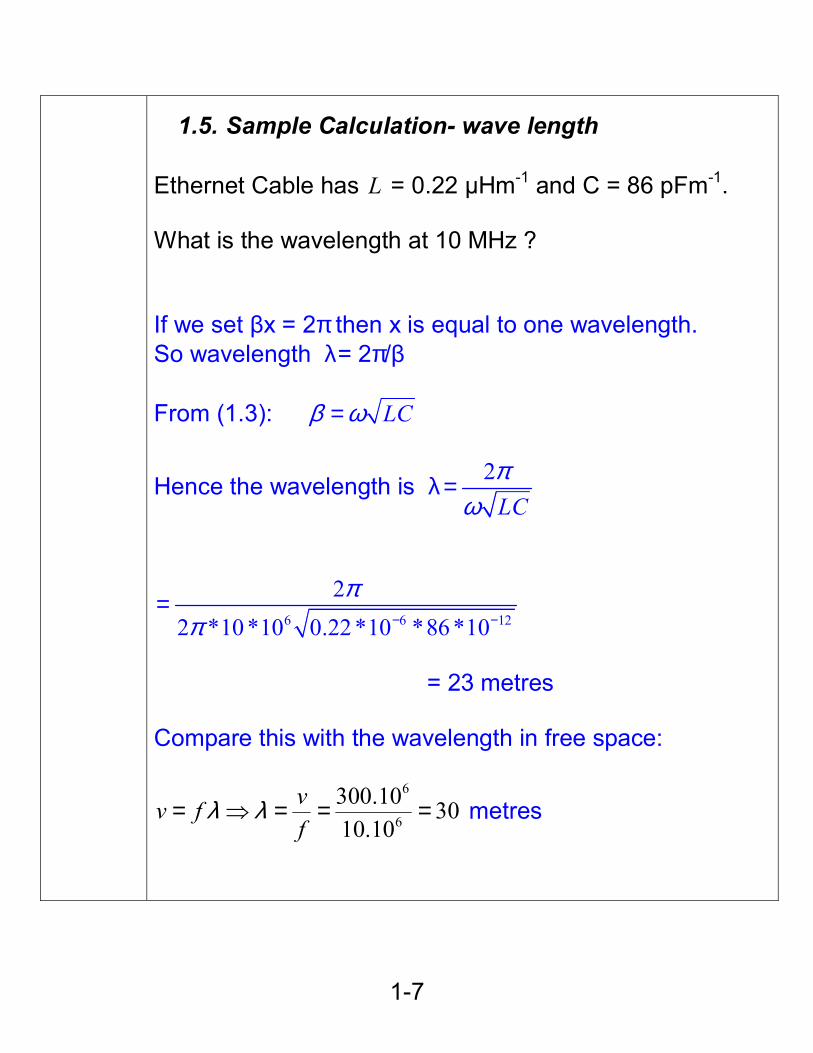
1.5. Sample Calculation- wave length Ethernet Cable has L = 0.22 µHm-1 and C = 86 pFm-1. What is the wavelength at 10 MHz ? If we set βx = 2π then x is equal to one wavelength. So wavelength λ= 2π/β From (1.3): LCβ ω=

Hence the wavelength is λ 2LCπ

ω=

6 6 12

22 *10 *10 0.22 *10 *86 *10

ππ − −

=

= 23 metres Compare this with the wavelength in free space:

6

6300.10 3010.10

vv ff

λ λ= ⇒ = = = metres

1-8

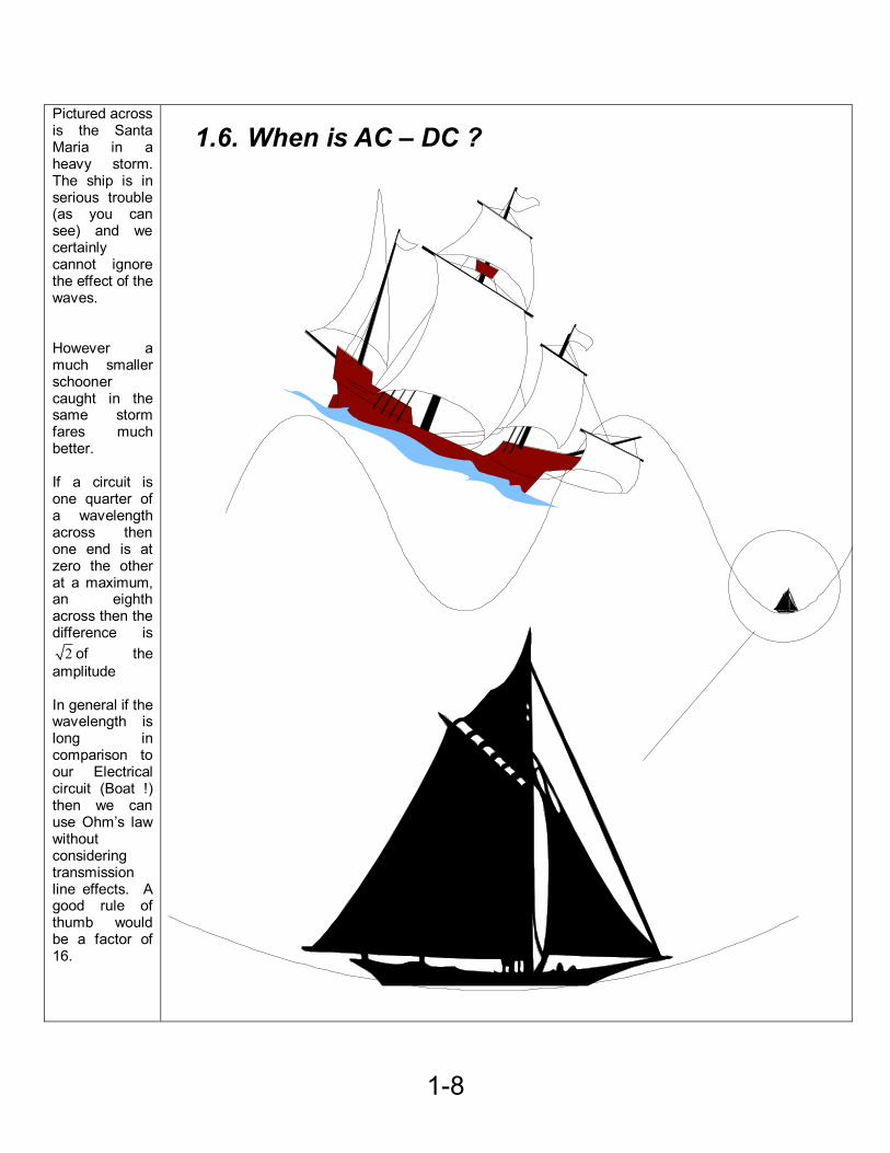
Pictured across is the Santa Maria in a heavy storm. The ship is in serious trouble (as you can see) and we certainly cannot ignore the effect of the waves. However a much smaller schooner caught in the same storm fares much better. If a circuit is one quarter of a wavelength across then one end is at zero the other at a maximum, an eighth across then the difference is

2 of the amplitude In general if the wavelength is long in comparison to our Electrical circuit (Boat !) then we can use Ohm’s law without considering transmission line effects. A good rule of thumb would be a factor of 16.

1.6. When is AC – DC ?

1-9

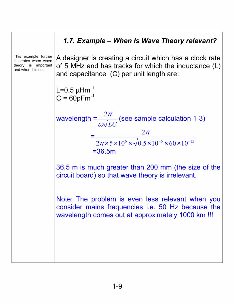
This example further illustrates when wave theory is important and when it is not.

1.7. Example – When Is Wave Theory relevant? A designer is creating a circuit which has a clock rate of 5 MHz and has tracks for which the inductance (L) and capacitance (C) per unit length are: L=0.5 µHm-1

C = 60pFm-1

wavelength = 2LCπ

ω(see sample calculation 1-3)

=6 6 12

22 5 10 0.5 10 60 10

ππ − −× × × × × ×

=36.5m 36.5 m is much greater than 200 mm (the size of the circuit board) so that wave theory is irrelevant. Note: The problem is even less relevant when you consider mains frequencies i.e. 50 Hz because the wavelength comes out at approximately 1000 km !!!

1-2

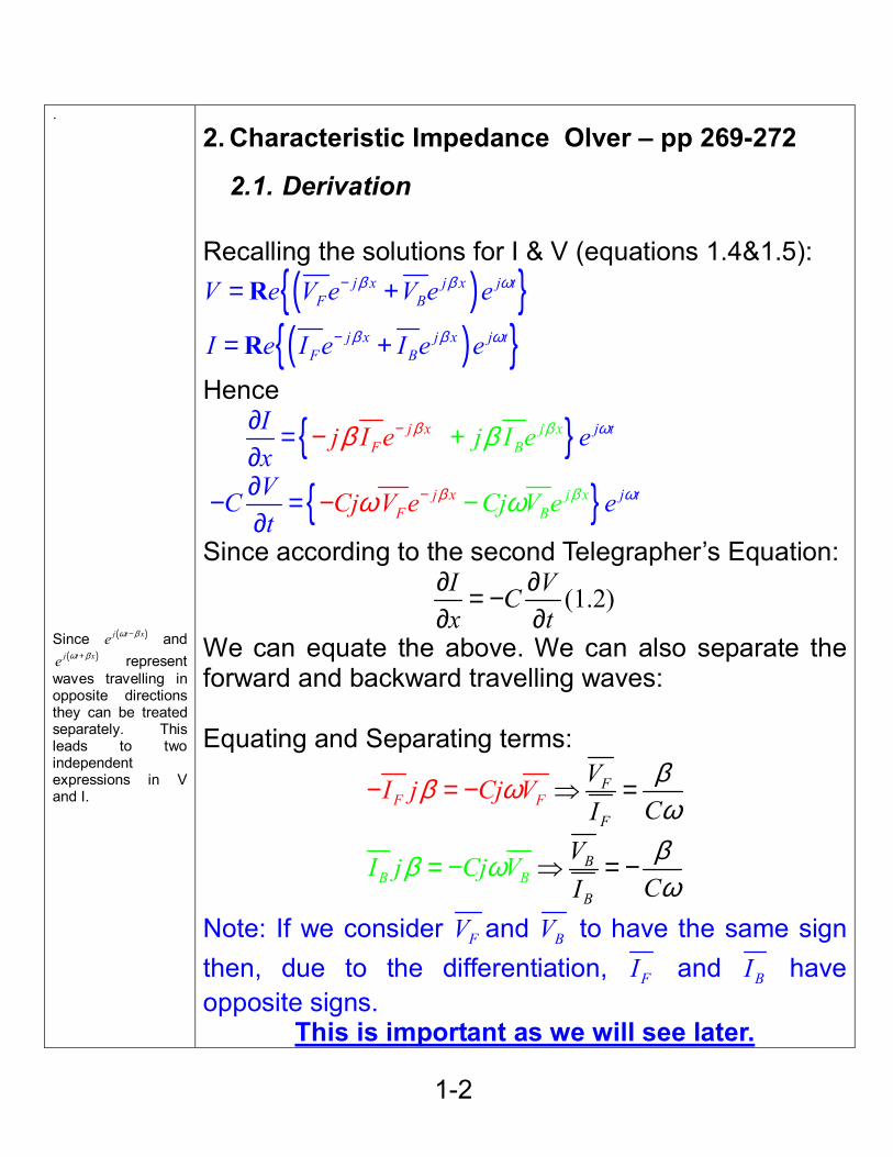
. Since ( )j t xe ω β− and

( )j t xe ω β+ represent waves travelling in opposite directions they can be treated separately. This leads to two independent expressions in V and I.

2. Characteristic Impedance Olver – pp 269-272

2.1. Derivation Recalling the solutions for I & V (equations 1.4&1.5):

( ) j x j x j tF BV e V e V e eβ β ω−= +R

( ) j x j x j tF BI e I e I e eβ β ω−= +R

Hence

j xF

j tB

jxI jj I ex

I ee β β ωββ − +∂∂

−=

jF

tj jx xBCjCVC e eV e

tVj β β ωωω −− −∂− =

∂

Since according to the second Telegrapher’s Equation:

(1.2)I VCx t

∂ ∂= −∂ ∂

We can equate the above. We can also separate the forward and backward travelling waves: Equating and Separating terms:

FF

FFI j Cj V V

CIβ β

ωω= − ⇒ =−

B BB

B

I j Cj V VCIβωω

β ⇒ = −= −

Note: If we consider FV and BV to have the same sign then, due to the differentiation, FI and BI have opposite signs.

This is important as we will see later.

2-3

IMPORTANT: A common misconception is to assume that the characteristic impedance Z0 is an impedance per unit length it is not: Z0 IS THE TOTAL IMPEDANCE, of a line of any length if there are no reflections. In the absence of reflections then the current and voltage are everywhere in phase. l and c are both real and hence so is z0. If there are reflections then the current and voltage of the advancing wave are again in phase but not (necessarily) with the current and voltage of the retreating wave. The line we have analysed has no resistors in it and yet z0 is ohmic. The characteristic impedance does not dissipate power it stores it.

The Characteristic impedance, z0 is defined as the ratio between the voltage and the current of a unidirectional wave on a transmission line at any point:

0F

F

VZI

=

z0 is always positive. From our expression in &F FI V overleaf and our definition of characteristic impedance it follows that:

0Z Cβ

ω=

and since: LCβ ω= ± (1.3)

0LZ C= (2.1)

2.2. Summarizing 1) For a unidirectional wave:- 0V Z I= at all points. 2) For any wave :- 0F FV Z I= and 0B BV Z I= − . Hence FV and FI are in phase BV and BI are in antiphase. 3) For a lossless line Z0 is real with units of ohms.

2-4

.

2.3. Characteristic Impedance – Example 1

Q - We wish to examine a circuit using an oscilloscope. The oscilloscope probe is on an infinitely long cable and has a characteristic impedance of 50 Ohm. What load does the probe add to the circuit? A - 1. Since the cable is infinitely long there are no reflections

2. For a wave with no reflections 0V ZI

= at all points, hence the probe

behaves like a load of 50 Ohms.

2.4. Characteristic Impedance – Example 2 Q – A wave of FV = 5 volts with a wavelength (λ) of 2 metres has a reflected wave of BV = 1 volts. If Z0 = 75 Ohms what are the voltage and current 3 metres from the end of the cable.

2πβ πλ

= =

From Equation 1.4 ---- xj xj

F BV V e V eβ β−= + X = - 3 Therefore ---- 3 35 j jV e e voltsπ π−= +

Also 0 0

xj xjF BV VI e eZ Z

β β−= −

3 35 175 75

j je e ampsπ π−= −

3-1

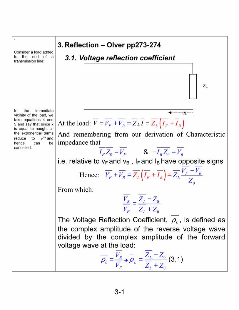
. Consider a load added to the end of a transmission line: In the immediate vicinity of the load, we take equations 4 and 5 and say that since x is equal to nought all the exponential terms reduce to j te ω and hence can be cancelled.

3. Reflection – Olver pp273-274

3.1. Voltage reflection coefficient

At the load: ( )LB BF L FV Z I Z IV IV= =+ = + And remembering from our derivation of Characteristic impedance that

0F FI Z V= & 0B BI Z V− = i.e. relative to vF and vB , IF and IB have opposite signs

Hence: ( )0

FF

BB BF L LZ I I V VV V Z

Z−+ = + =

From which: 0

0

B L

F L

V Z ZV Z Z

−=+

The Voltage Reflection Coefficient, Lρ , is defined as the complex amplitude of the reverse voltage wave divided by the complex amplitude of the forward voltage wave at the load:

BL

F

VV

ρ = 0

0

LL

L

Z ZZ Z

ρ −=+

(3.1)

-X

ZL

3-2

*I is the complex conjugate. If

*

I A jBthen

I A jB

= +

= −

*I and V are peak values, power is calculated on RMS hence the factor of ½. This is the power dissipated in the load so it is reduced by any value of Lρ greater than nought. Hence that power must be being reflected back down the line which is logical bearing in mind

Lρ is defined as the proportion of the voltage reflected back.

3.2. Power Reflection Mean Power dissipated in any load :

*1 Re2

V I

At the load:

0

(1 )

(1 )

F L

FL

V

VI

V

Z

ρ

ρ

=

=

+

−

Hence:

( )( )2

* *

0

1 1 1 12 2

FL L

VV I

Zρ ρ= + −

( )2

2*

0

12F

L L L

V

Zρ ρ ρ= + − −

but *

L Lρ ρ− is imaginary so:

( )2

2*

0

1 Re 12 2

FL

VV I

Zρ= −

Therefore: The fraction of power reflected from the load is:

2

Lρ

3-3

. If there is total reflection then Lρ is 1 and the VSWR is infinite. Zero reflection leads to a VSWR of 1 Standing waves can be detected by measuring voltages along a transmission line.

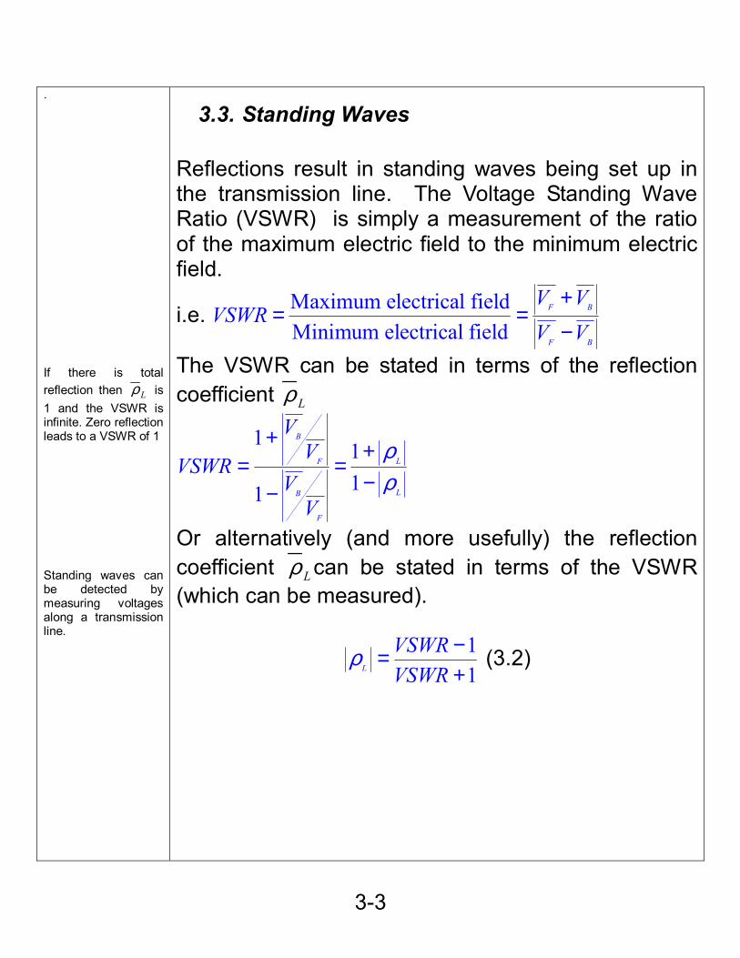
3.3. Standing Waves Reflections result in standing waves being set up in the transmission line. The Voltage Standing Wave Ratio (VSWR) is simply a measurement of the ratio of the maximum electric field to the minimum electric field.

i.e. Maximum electrical fieldMinimum electrical field

F B

F B

V VVSWR

V V+

= =−

The VSWR can be stated in terms of the reflection coefficient Lρ

1 111

B

LF

LB

F

VV

VSWRVV

ρρ

+ += =

−−

Or alternatively (and more usefully) the reflection coefficient Lρ can be stated in terms of the VSWR (which can be measured).

11L

VSWRVSWR

ρ −=+

(3.2)

3-4

i.e. that the load is equal to the characteristic impedance.

3.4. Summarizing For full power transfer we require 0Lρ =

When 0Lρ = a load is said to be “matched”

The advantages of matching are that:

1) We get all the power to the load 2) There are no echoes

The simplest way to match a line to a load is to set:

0 LZ Z= Since -

Voltage reflection coefficient is 0

0

LL

L

Z ZZ Z

ρ −=+

Fraction of power reflected = 2

Lρ

Reflections will set up standing waves (in just the same way as you get with optical waves). The Voltage Standing Wave Ratio (VSWR) is given by:

( )( )11

L

L

VSWRρρ

+=

−

3-5

3.5. Example - Termination (e.g. of BNC lines) We know that the characteristic impedance of a cable is given by:

0 (2.1)LZ C= and we know that the voltage reflection coefficient is:

0

0

(3.1)LL

L

Z ZZ Z

ρ −=+

So in order to avoid unwanted reflections we need a ZL to terminate our coaxial cable which has the same impedance as the characteristic impedance of the cable. The capacitance per unit length of a coaxial cable is given by

02ln( / )

rCb a

πε ε=

Where b is the outside diameter and a is the inside diameter.

3-6

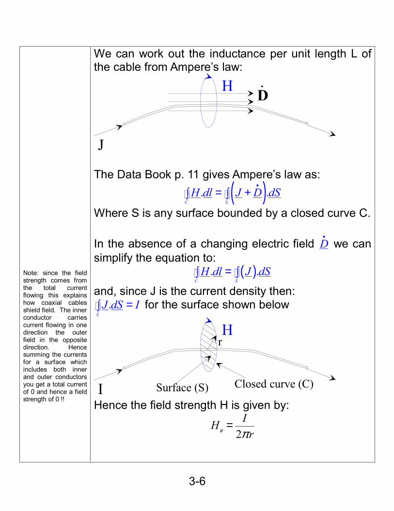
Note: since the field strength comes from the total current flowing this explains how coaxial cables shield field. The inner conductor carries current flowing in one direction the outer field in the opposite direction. Hence summing the currents for a surface which includes both inner and outer conductors you get a total current of 0 and hence a field strength of 0 !!

We can work out the inductance per unit length L of the cable from Ampere’s law:

J

DH .

The Data Book p. 11 gives Ampere’s law as:

( ). ..

C S

H dl J D dS= +∫ ∫

Where S is any surface bounded by a closed curve C. In the absence of a changing electric field

.D we can

simplify the equation to: ( ). .

C S

H dl J dS=∫ ∫

and, since J is the current density then: .

S

J dS I=∫ for the surface shown below

I

H

Surface (S) Closed curve (C)

r

Hence the field strength H is given by:

2IHrφ π

=

3-7

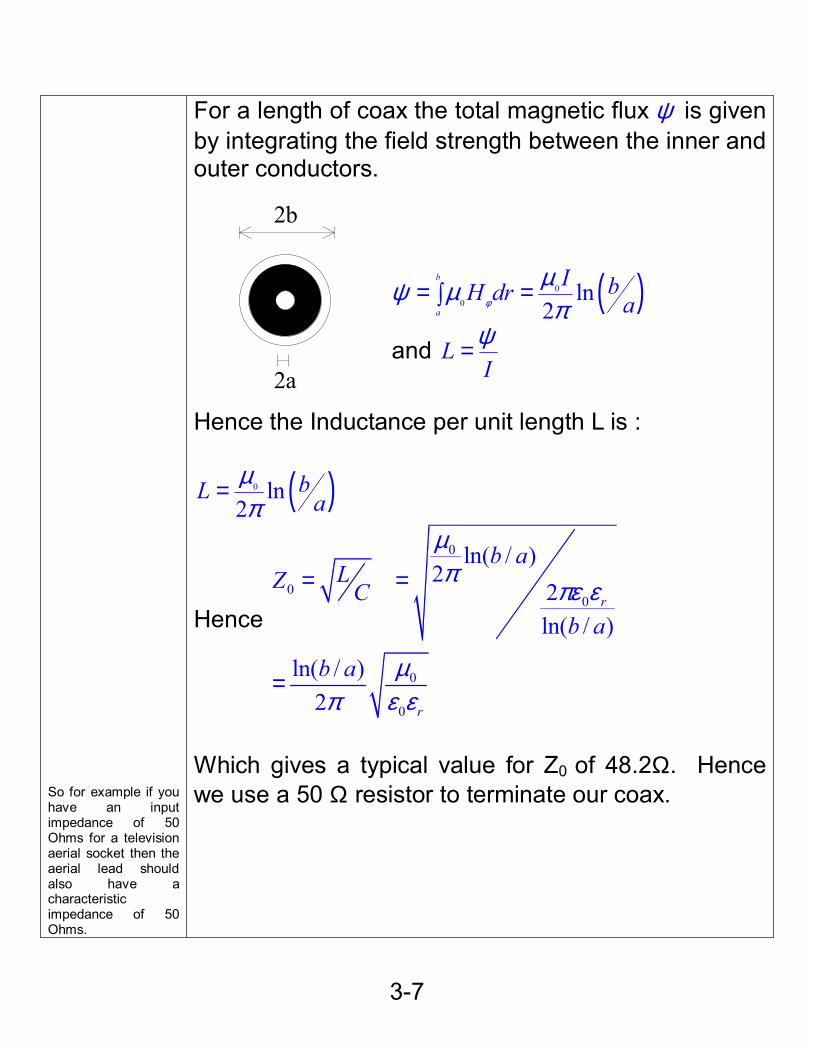
So for example if you have an input impedance of 50 Ohms for a television aerial socket then the aerial lead should also have a characteristic impedance of 50 Ohms.

For a length of coax the total magnetic flux ψ is given by integrating the field strength between the inner and outer conductors.

( )00 ln

2b

a

I bH dr aφ

µψ µπ

= =∫

and LI

ψ=

Hence the Inductance per unit length L is :

( )0 ln2

bL aµπ

=

Hence

0

00

0

0

ln( / )2

2ln( / )

ln( / )2

r

r

b aLZ C

b a

b a

µπ

πε ε

µπ ε ε

= =

=

Which gives a typical value for Z0 of 48.2Ω. Hence we use a 50 Ω resistor to terminate our coax.

2b

2a

3-8

.

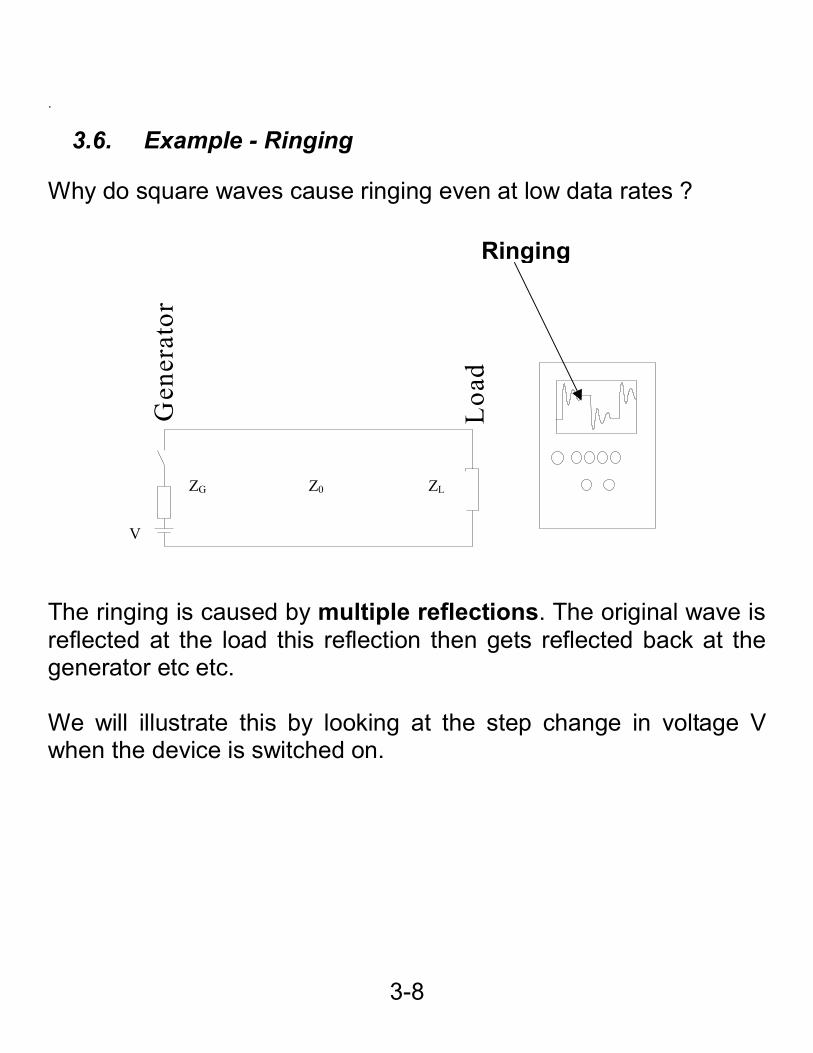
3.6. Example - Ringing Why do square waves cause ringing even at low data rates ?

Gen

erat

or

Loa

d

The ringing is caused by multiple reflections. The original wave is reflected at the load this reflection then gets reflected back at the generator etc etc. We will illustrate this by looking at the step change in voltage V when the device is switched on.

ZG Z0 ZL

V

Ringing

3-9

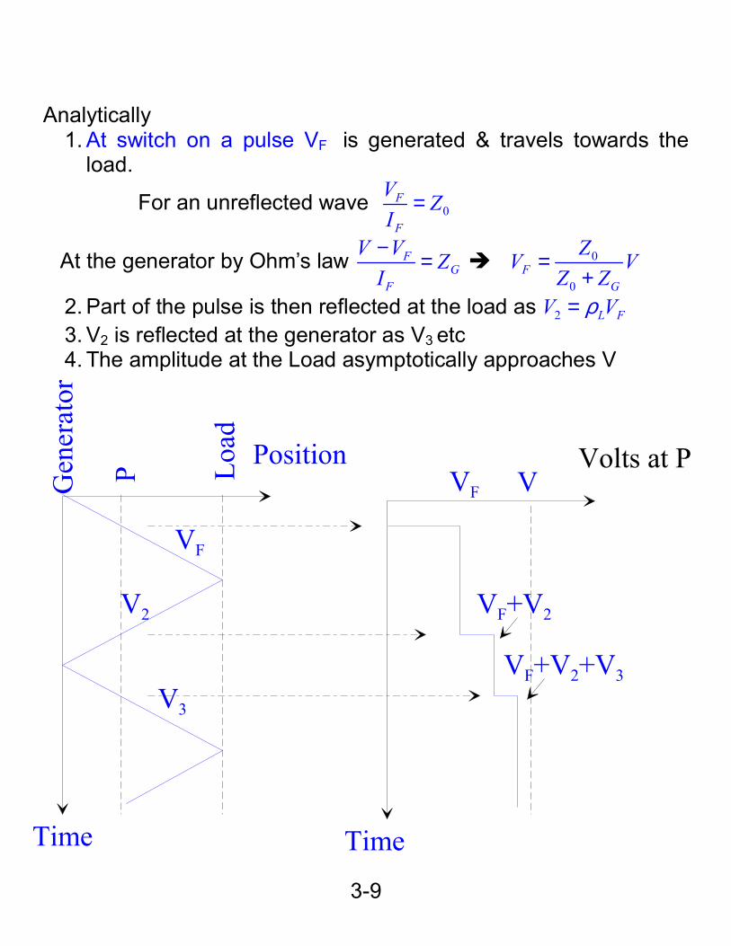
Analytically

1. At switch on a pulse VF is generated & travels towards the load.

For an unreflected wave 0F

F

V ZI

=

At the generator by Ohm’s law FG

F

V V ZI− = 0

0F

G

ZV VZ Z

=+

2. Part of the pulse is then reflected at the load as 2 L FV Vρ= 3. V2 is reflected at the generator as V3 etc 4. The amplitude at the Load asymptotically approaches V

P Load Position

Time Time

VF

VF+V2

VVolts at P

VF+V2+V3

VF

V2

V3

Gen

erat

or

3-10

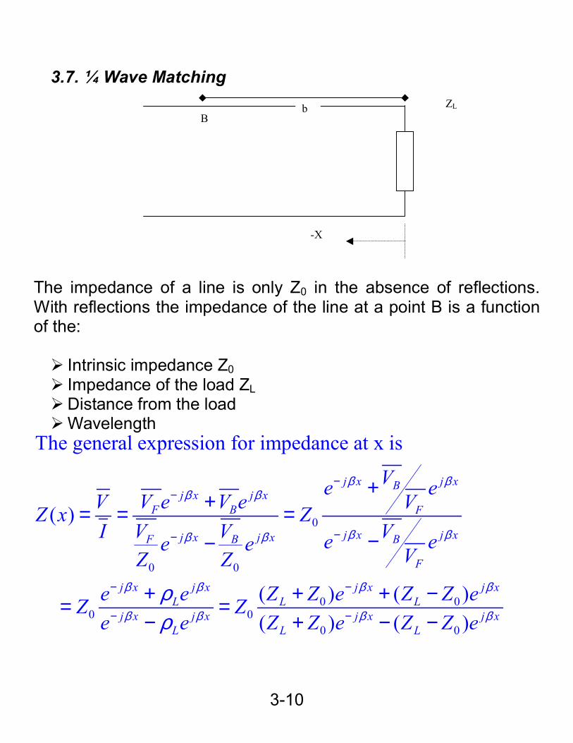
3.7. ¼ Wave Matching

The impedance of a line is only Z0 in the absence of reflections. With reflections the impedance of the line at a point B is a function of the: Intrinsic impedance Z0 Impedance of the load ZL Distance from the load Wavelength

0

0 0

0 00 0

0 0

The general expression for impedance at x is

( )

( ) ( )( ) ( )

j x j xBj x j x

F B F

j x j xj x j xF B B

F

j x j x j x j xL L L

j x j x j x j xL L L

Ve eV V e V e VZ x ZI V V Ve ee e VZ Z

e e Z Z e Z Z eZ Ze e Z Z e Z Z e

β ββ β

β ββ β

β β β β

β β β βρρ

−−

−−

− −

− −

++= = =

−−

+ + + −= =− + − −

ZL

-X

B b

3-11

( )( )

00

0

00

0

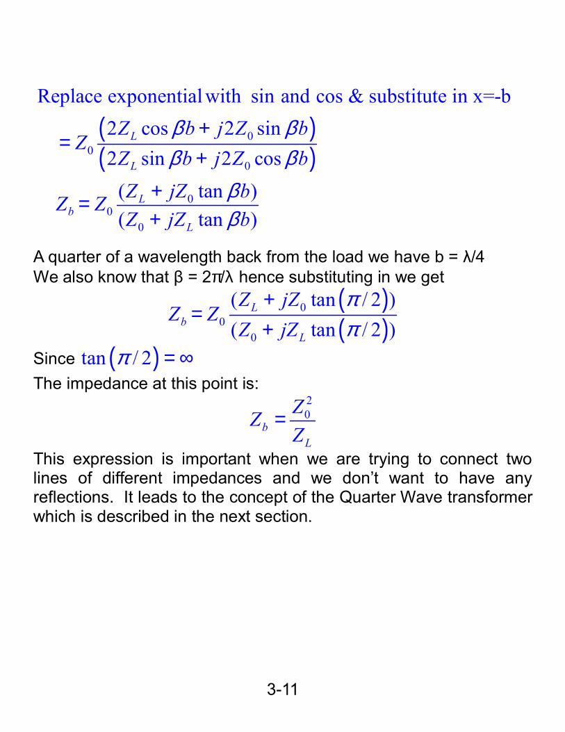
Replace exponential with sin and cos & substitute in x=-b2 cos 2 sin2 sin 2 cos

( tan )( tan )

L

L

Lb

L

Z b j Z bZ

Z b j Z bZ jZ bZ ZZ jZ b

β ββ β

ββ

+=

++=+

A quarter of a wavelength back from the load we have b = λ/4 We also know that β = 2π/λ hence substituting in we get

( )( )

00

0

( tan / 2 )( tan / 2 )

Lb

L

Z jZZ Z

Z jZππ

+=

+

Since ( )tan / 2π = ∞ The impedance at this point is:

20

bL

ZZZ

=

This expression is important when we are trying to connect two lines of different impedances and we don’t want to have any reflections. It leads to the concept of the Quarter Wave transformer which is described in the next section.

3-12

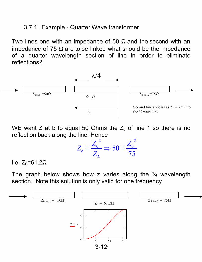
3.7.1. Example - Quarter Wave transformer Two lines one with an impedance of 50 Ω and the second with an impedance of 75 Ω are to be linked what should be the impedance of a quarter wavelength section of line in order to eliminate reflections? WE want Z at b to equal 50 Ohms the Z0 of line 1 so there is no reflection back along the line. Hence

2 20 050

75bL

Z ZZZ

= ⇒ =

i.e. Z0=61.2Ω

The graph below shows how z varies along the ¼ wavelength section. Note this solution is only valid for one frequency.

λ/4

Z0line 1=50Ω Z0 line 2=75Ω Z0=??

b Second line appears as ZL = 75Ω to the ¼ wave link

Z0line 1 = 50Ω Z0 line 2 = 75Ω Z0 = 61.2Ω

2 2.5 350

60

70

Zb ( )b

.β b

3-1

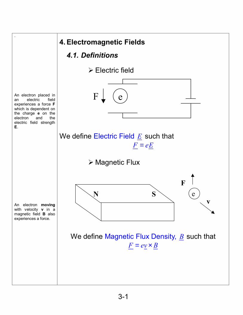
. An electron placed in an electric field experiences a force F which is dependent on the charge e on the electron and the electric field strength E. An electron moving with velocity v in a magnetic field B also experiences a force.

4. Electromagnetic Fields

4.1. Definitions

Electric field We define Electric Field E such that

F eE=

Magnetic Flux

We define Magnetic Flux Density, B such that F ev B= ×

eF

N S e F

v

4-2

As we can see electric fields and magnetic fields are closely related. One can give rise to the other and vice versa Permittivities and permeabilities are often expressed relative to that of free space e.g. ε=ε0εr . Where ε0 is he permeabilitiy of free space. Note: The electric field and magnetic field equations have been deliberately formulated to appear similar.

Electric fields are not only created by charge (such as the charge on the plates of a capacitor) but also by a changing magnetic field. Magnetic fields are created not only by moving charges i.e. current in a coil or aligned spins in an atom (as in a permanent magnet), but also by changing electric fields (this is Maxwells Displacement current which we will discuss later)

In addition to the above we have to allow for the charges and currents in materials and for this we define two new quanitities:

Electric Flux : D

Magnetic Field : H

In Linear materials D and E and B and H are directly related by the permittivity ε and permeability µ of the material

D= εE

H=B/µ

4-3

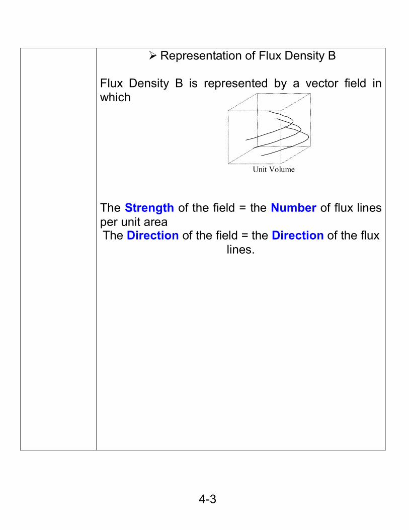
Representation of Flux Density B Flux Density B is represented by a vector field in which The Strength of the field = the Number of flux lines per unit area The Direction of the field = the Direction of the flux

lines.

Unit Volume

4-4

We will be using both the Maxwell-Faraday and the Maxwell-Ampere laws later in the lectures to derive the equations for Electromagnetic waves in free space.

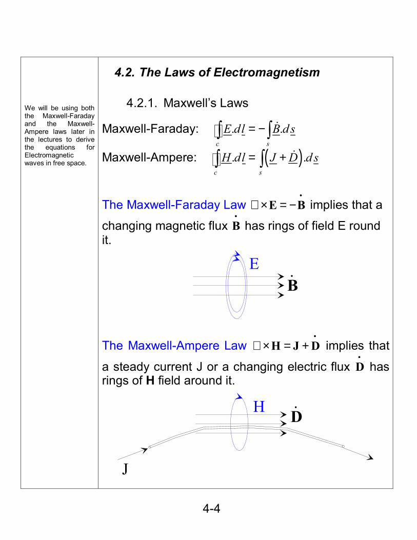
4.2. The Laws of Electromagnetism

4.2.1. Maxwell’s Laws

Maxwell-Faraday: . .c s

E dl B d s= −∫ ∫ &

Maxwell-Ampere: ( ). .c s

H dl J D d s= +∫ ∫ &

The Maxwell-Faraday Law •

∇ × = −E B implies that a

changing magnetic flux •B has rings of field E round

it.

The Maxwell-Ampere Law •

∇ × = +H J D implies that

a steady current J or a changing electric flux •D has

rings of H field around it.

BE .

J

DH .

4-5

If the divergence of B is zero then that implies that the flux lines which are used to represent the flux density are continuous i.e. unbroken loops

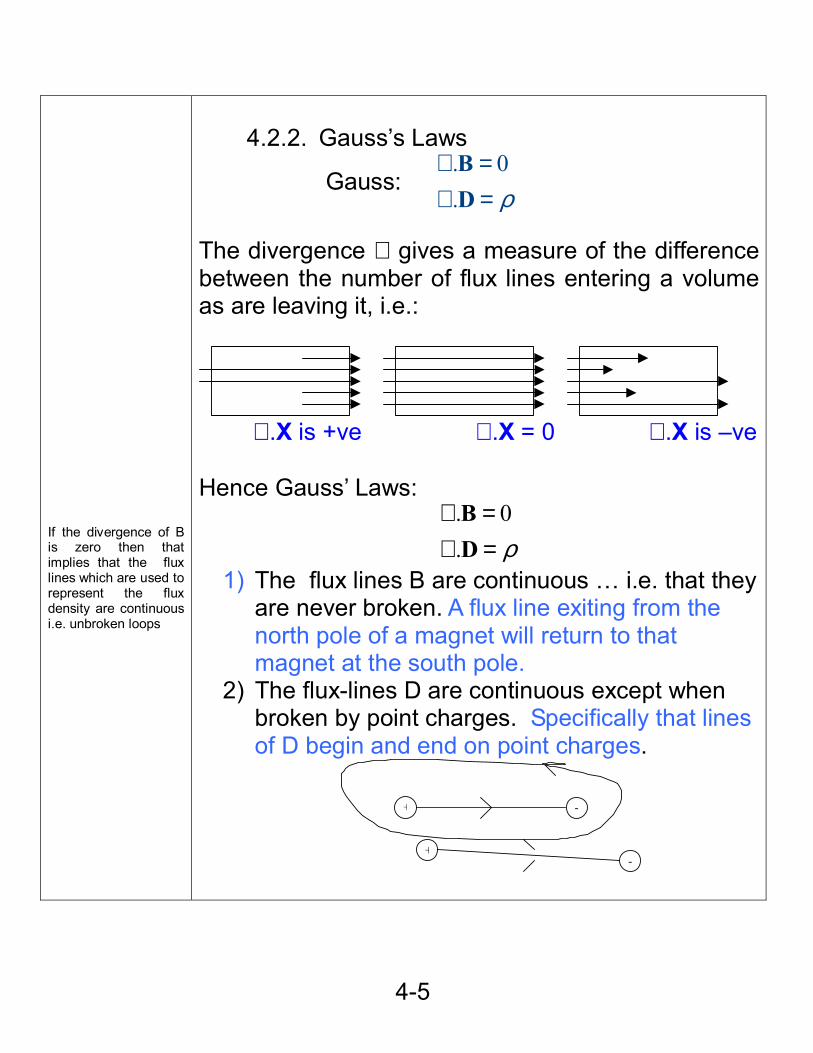
4.2.2. Gauss’s Laws

Gauss: . 0. ρ

∇ =∇ =

BD

The divergence ∇ gives a measure of the difference between the number of flux lines entering a volume as are leaving it, i.e.:

∇ .X is +ve ∇ .X = 0 ∇ .X is –ve Hence Gauss’ Laws:

. 0

. ρ∇ =∇ =

BD

1) The flux lines B are continuous … i.e. that they are never broken. A flux line exiting from the north pole of a magnet will return to that magnet at the south pole.

2) The flux-lines D are continuous except when broken by point charges. Specifically that lines of D begin and end on point charges.

+ -

+-

4-1

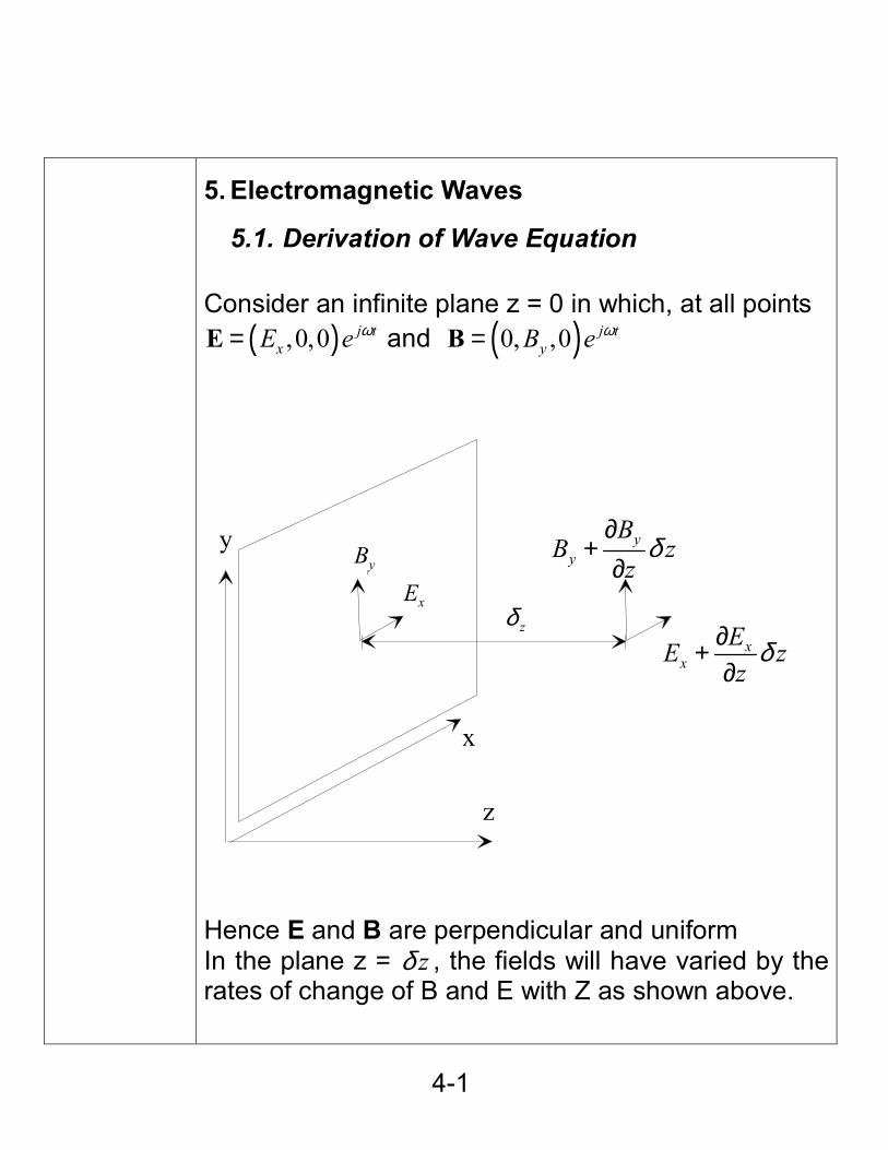
5. Electromagnetic Waves

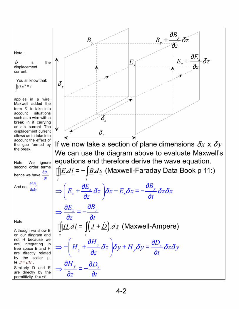
5.1. Derivation of Wave Equation Consider an infinite plane z = 0 in which, at all points

( ),0,0 j txE e ω=E and ( )0, ,0 j t

yB e ω=B

Hence E and B are perpendicular and uniform In the plane z = zδ , the fields will have varied by the rates of change of B and E with Z as shown above.

yB

xx

EE zz

δ∂+∂

yy

BB z

zδ

∂+

∂

zδ

x

y

z

xE

4-2

Note : D& is the displacement current. You all know that:

.c

H dl I=∫

applies in a wire. Maxwell added the term D& to take into account situations such as a wire with a break in it carrying an a.c. current. The displacement current allows us to take into account the effect of the gap formed by the break. Note: We ignore second order terms

hence we have yBt

∂∂

And not 2

yBt z

∂∂ ∂

Note: Although we show B on our diagram and not H because we are integrating in free space B and H are directly related by the scalar µ. Ie, B Hµ= . Similarly D and E are directly by the permittivity D Eε=

If we now take a section of plane dimensions xδ x yδWe can use the diagram above to evaluate Maxwell’s equations end therefore derive the wave equation.

. .c s

E dl B d s= −∫ ∫ & (Maxwell-Faraday Data Book p 11:)

yxx x

yx

BEE z x E x z xz tBE

z t

δ δ δ δ δ∂∂ ⇒ + − = − ∂ ∂

∂∂⇒ = −

∂ ∂

( ). .c s

H dl J D d s= +∫ ∫ & (Maxwell-Ampere)

y xy y

y x

H DH z y H y z yz t

H Dz t

δ δ δ δ δ∂ ∂

⇒ − + + = ∂ ∂ ∂ ∂

⇒ = −∂ ∂

yB

xEx

xEE zz

δ∂+∂

yy

BB z

zδ

∂+

∂

yδ

xδ

zδ

4-3

Wave velocity is defined by:

1 1. .velocity c flcµε

=

This agreed with the measured value and help substantiate the theory.

The next step is to eliminate B from the first equation and D from the second. Since B H and D Eµ ε= = : We get the following equations in E and H:

yx HEz t

µ∂∂ = −

∂ ∂ (5.1)

y xH Ez t

ε∂ ∂= −∂ ∂

(5.2)

These are exactly similar to the Telegrapher’s Equations:

V ILx t

∂ ∂= −∂ ∂

(1.7) I VCx t

∂ ∂= −∂ ∂

(1.8)

Applying the same technique of differentiating eq. 5.1 and substituting in from 5.2 and vice versa we end up with the equations for electromagnetic waves in free space.

2 2

2 2. . .Ht

E Ez tz

µ µ ε∂ ∂ − ∂ ∂∂

∂=

=∂ ∂

2 2

2 2. . .Et

H Hz tz

ε µ ε∂ ∂ − ∂ ∂∂

∂=

=∂ ∂

Which have the same form and therefore similar solutions to the equations for waves in transmission lines. All of the results which we obtained from the Telegrapher’s Equations can be reused for the equations for Electromagnetic waves.

5-4

Note: The vectors E and H are orthogonal to one another hence the subscripts x and y in our expression for η.

5.2. Intrinsic Impedance

For EM Waves We define a quantity: η = the intrinsic impedance. is a function of the permeability and the permittivity in the same way that Z the characteristic impedance was a function of the inductance and capacitances per unit length.

0

(5.3)

c.f. (2.1)LZ C

µη ε=

=

η links E & H in the same way that Z the characteristic impedance linked V & I.

c. f. xF xB

yF B

B

By

F

F

V VZE EH IH I

η = = −= = −

6-1

6. Reflection and refraction of waves

6.1. Reflection of Incident wave normal to the plane of the reflection

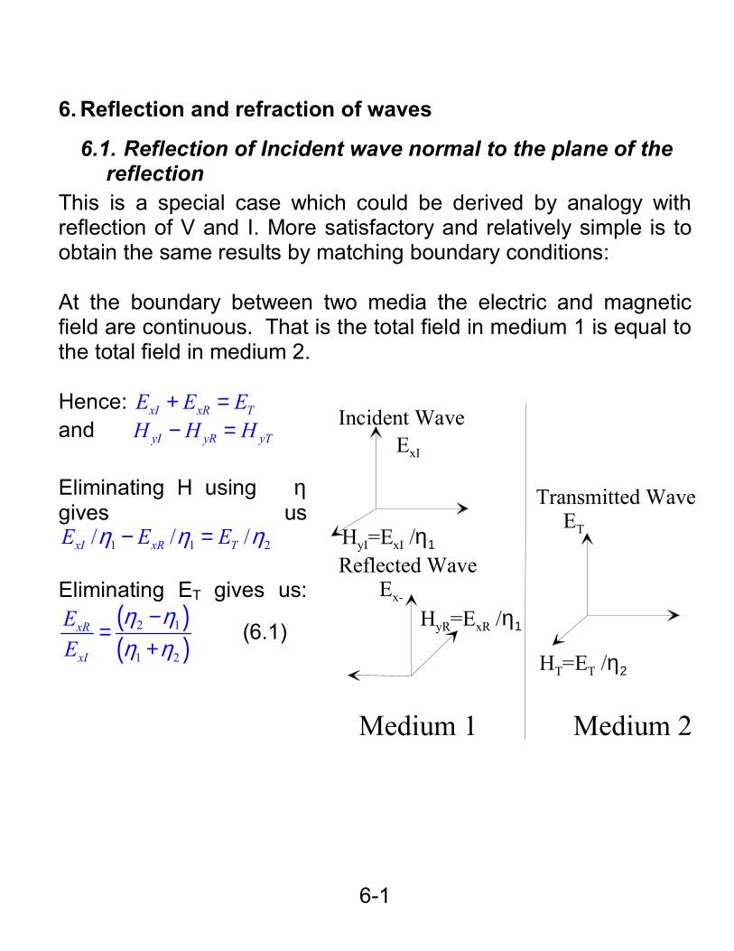
This is a special case which could be derived by analogy with reflection of V and I. More satisfactory and relatively simple is to obtain the same results by matching boundary conditions: At the boundary between two media the electric and magnetic field are continuous. That is the total field in medium 1 is equal to the total field in medium 2. Hence: xI xR TE E E+ = and yI yR yTH H H− = Eliminating H using η gives us

1 1 2/ / /xI xR TE E Eη η η− = Eliminating ET gives us:

( )( )

2 1

1 2

xR

xI

EE

η ηη η

−=

+ (6.1)

Incident Wave

Transmitted Wave

Reflected Wave

ExI

HyI=ExI /η1

Ex-

HyR=ExR /η1

HT=ET /η2

ET

Medium 1 Medium 2

6-2

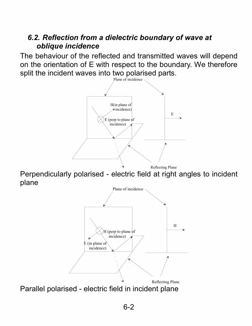
6.2. Reflection from a dielectric boundary of wave at oblique incidence

The behaviour of the reflected and transmitted waves will depend on the orientation of E with respect to the boundary. We therefore split the incident waves into two polarised parts.

E (perp to plane of incidence)

H(in plane of incidence)

Plane of incidence

Reflecting Plane

E

Perpendicularly polarised - electric field at right angles to incident plane

H (perp to plane of incidence)

E (in plane of incidence)

Plane of incidence

Reflecting Plane

H

Parallel polarised - electric field in incident plane

6-3

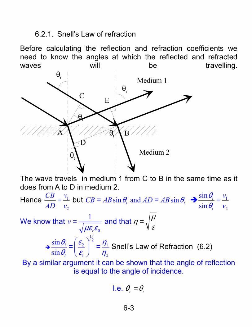
6.2.1. Snell’s Law of refraction

Before calculating the reflection and refraction coefficients we need to know the angles at which the reflected and refracted waves will be travelling.

θi

A

C E

DB

θt

θt

θi

θr

Medium 1

Medium 2

The wave travels in medium 1 from C to B in the same time as it does from A to D in medium 2.

Hence 1

2

CB vAD v

= but sin and sini tCB AB AD ABθ θ= = 1

2

sinsin

i

t

vv

θθ

=

We know that 0

1

r

vµε ε

= and that µηε

=

12

2 1

1 2

sinsin

i

t

θ ε ηθ ε η

= =

Snell’s Law of Refraction (6.2)

By a similar argument it can be shown that the angle of reflection is equal to the angle of incidence.

I.e. r iθ θ=

6-4

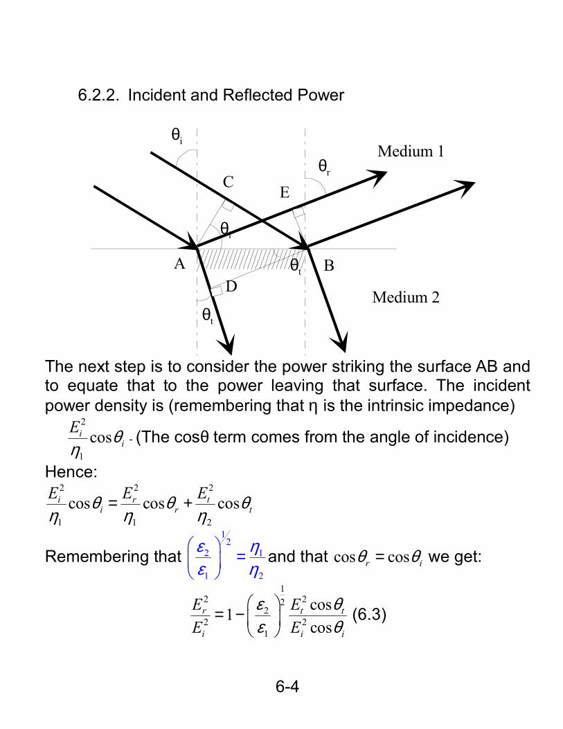
6.2.2. Incident and Reflected Power

θi

A

C E

DB

θt

θt

θi

θr

Medium 1

Medium 2

The next step is to consider the power striking the surface AB and to equate that to the power leaving that surface. The incident power density is (remembering that η is the intrinsic impedance)

2

1

cosii

E θη

- (The cosθ term comes from the angle of incidence)

Hence: 2 2 2

1 1 2

cos cos cosi r ti r t

E E Eθ θ θη η η

= +

Remembering that 1

22 1

1 2

ε ηε η

=

and that cos cosr iθ θ= we get:

12 22

22 2

1

cos1cos

r t t

i i i

E EE E

ε θε θ

= −

(6.3)

6-5

6.2.3. Perpendicularly polarised waves

Having got our expression for power we can consider the two sets of waves starting with the perpendicularly polarised waves. In these waves the electric field is perpendicular to the plane of incidence i.e. parallel to the boundary between the two media. Summing the electric fields we get

t r iE E E= + Combining this with equation 6.3 which was:

12 2 22

22 2 2

1

cos1 1cos

R T T T

I I I I

E E EkE E E

ε θε θ

= − = −

Where 12

2

1

coscos

t

i

k ε θε θ

=

We get the following:

( ) ( )2 22

2 1 1 (1 ) 2 1 0R R R R

I I I I

E E E Ek k k kE E E E

= − + ⇒ + + + − =

Hence: 1 1

2 21 21 1

2 21 2

cos cos = cos cos

R I T

I I T

EE

ε θ ε θε θ ε θ

− +

This expression contains the angle of the transmitted wave, however we can use Snell’s law to obtain a more useful expression which contains only the angle of incidence. I.e.

( )( )

1/ 222

11/ 2

22

1

cos sin= (6.4)

cos sin

I IR

II I

EE

εθ θεεθ θε

− − + −

6-6

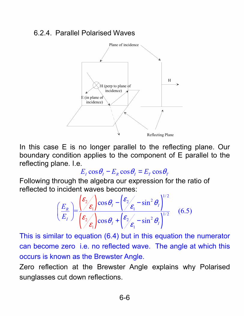
6.2.4. Parallel Polarised Waves

H (perp to plane of incidence)

E (in plane of incidence)

Plane of incidence

Reflecting Plane

H

In this case E is no longer parallel to the reflecting plane. Our boundary condition applies to the component of E parallel to the reflecting plane. I.e.

cos cos cosI I R I T TE E Eθ θ θ− = Following through the algebra our expression for the ratio of reflected to incident waves becomes:

( ) ( )( ) ( )

1/ 222

11/

2

1

11

222

2

cos sin= (6.5)

cos sin

I IR

II I

EE

εε

ε

εθ θεε θε θ ε

− − + −

This is similar to equation (6.4) but in this equation the numerator can become zero i.e. no reflected wave. The angle at which this occurs is known as the Brewster Angle. Zero reflection at the Brewster Angle explains why Polarised sunglasses cut down reflections.

6-7

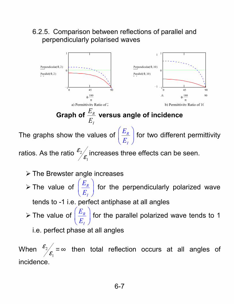
6.2.5. Comparison between reflections of parallel and perpendicularly polarised waves

Graph of R

I

EE

versus angle of incidence

The graphs show the values of R

I

EE

for two different permittivity

ratios. As the ratio 2

1

εε increases three effects can be seen.

The Brewster angle increases

The value of R

I

EE

for the perpendicularly polarized wave

tends to -1 i.e. perfect antiphase at all angles

The value of R

I

EE

for the parallel polarized wave tends to 1

i.e. perfect phase at all angles When 2

1

εε = ∞ then total reflection occurs at all angles of

incidence.

0 45 901

0

1

a) Permittivity Ratio of 2

Perpendicular( ),θ 2

Parallel( ),θ 2

.θ180π

0 45 901

0

1

b) Permittivity Ratio of 10

1

1

Perpendicular( ),θ 10

Parallel( ),θ 10

900 .θ180π

6-8

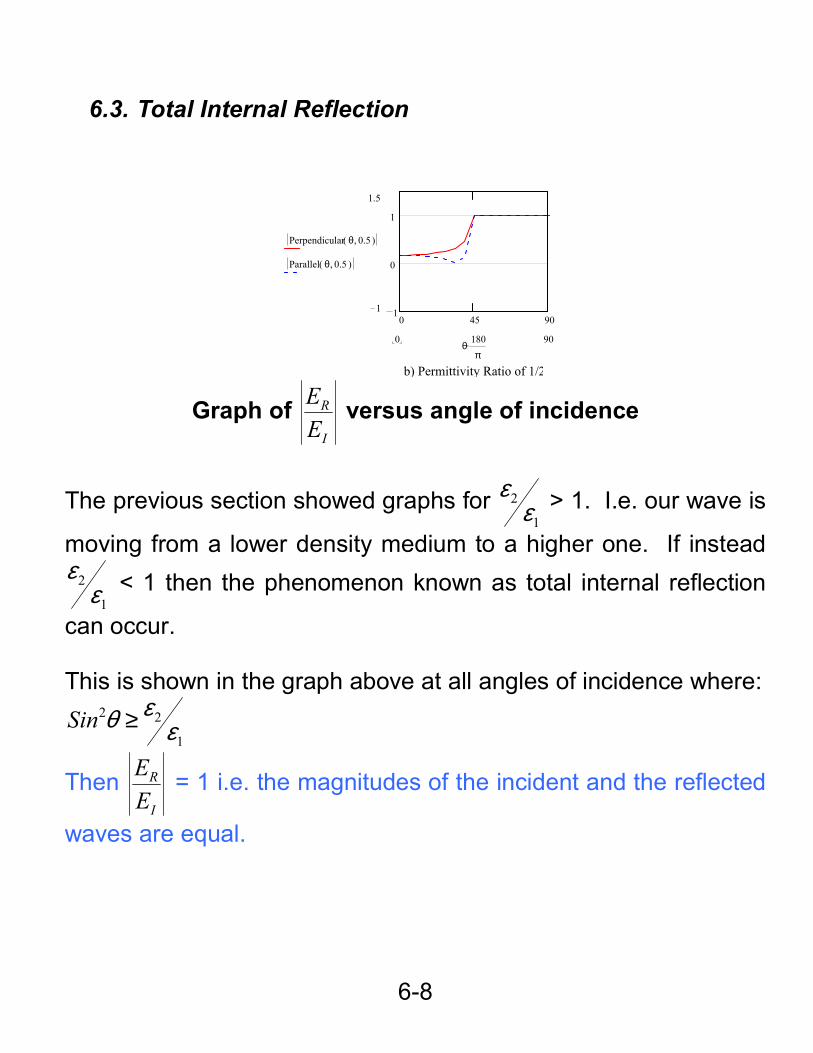
6.3. Total Internal Reflection

Graph of R

I

EE

versus angle of incidence

The previous section showed graphs for 2

1

εε > 1. I.e. our wave is

moving from a lower density medium to a higher one. If instead 2

1

εε < 1 then the phenomenon known as total internal reflection

can occur. This is shown in the graph above at all angles of incidence where:

2 2

1Sin εθ ε≥

Then R

I

EE

= 1 i.e. the magnitudes of the incident and the reflected

waves are equal.

0 45 901

0

1

b) Permittivity Ratio of 1/2

1.5

1

Perpendicular( ),θ 0.5

Parallel( ),θ 0.5

900 .θ180π

6-9

6.4. Comparison of Transmission Line & Free Space Waves Symbols: V: Voltage Volts E Electric Field Volts m-1

I: Current Amps H Magnetic Field Amps m-1

l: Inductance Henry m-1 µ permeability Henry m-1

c: Capacitance Farad m-1 ε Permittivity Farad m-1

Z Characteristic impedance

Ohms η Intrinsic impedance Ohms

Equations: ( ) ( ) j t x j t x

F BV e V e V eω β ω β− += +R ( ) ( ) j t z j t zx xF xBE e E e E eω β ω β− += +R

( ) ( ) j t x j t xF BI e I e I eω β ω β− += +R ( ) ( ) j t z j t z

y yF yBH e H e H eω β ω β− += +R

0F B

F B

V V Lz CI I= − = = xF xB

yF yB

E EH H

µη ε= − = =

Wave velocity 1LC

= Wave Velocity 1µε

=

LCβ ω= β ω µε=

0

0

LBL

LF

V Z ZV Z Z

ρ −= =+

2 1

2 1

xBL

xF

EE

η ηρη η

−= =+

Power Reflection 2Lρ= Power Reflection 2

Lρ=

Wave Power *1Re

2V I =

Wave Power

*1Re2E H = ×

ω: Frequency, radians s-1, β: Spatial frequency, radians m-1Note

The Wave Power ( )* 21 Re2

E H Wm−= × is the complex Poynting

Vector and will be derived in the next lecture

6-10

.

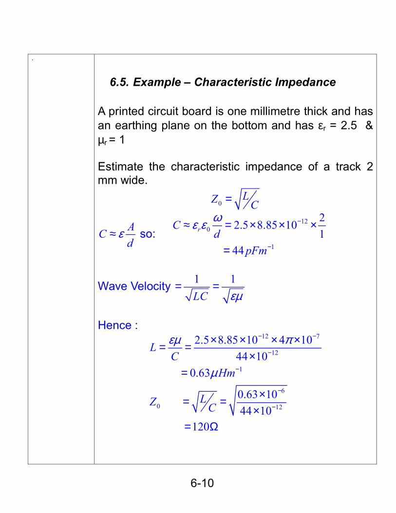
6.5. Example – Characteristic Impedance A printed circuit board is one millimetre thick and has an earthing plane on the bottom and has εr = 2.5 & µr = 1 Estimate the characteristic impedance of a track 2 mm wide.

0LZ C=

ACd

ε≈ so: 12

0

1

22.5 8.85 101

44

rCd

pFm

ωε ε −

−

≈ = × × ×

=

Wave Velocity 1 1LC εµ

= =

Hence :

12 7

12

1

6

0 12

2.5 8.85 10 4 1044 10

0.63

0.63 1044 10

120

LC

Hm

LZ C

εµ π

µ

− −

−

−

−

−

× × × ×= =×

=

×= =×

= Ω

6-11

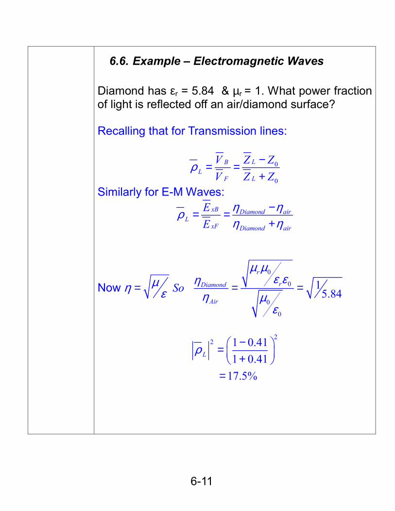
6.6. Example – Electromagnetic Waves Diamond has εr = 5.84 & µr = 1. What power fraction of light is reflected off an air/diamond surface? Recalling that for Transmission lines:

0

0

LBL

LF

V Z ZV Z Z

ρ −= =+

Similarly for E-M Waves: xB Diamond air

LxF Diamond air

EE

η ηρη η

−= =+

Now 0

0

0

0

15.84

r

rDiamond

Air

So

µ µε εηµη ε η µε

= = =

2

2 1 0.411 0.41

17.5%

Lρ − = + =

6-1

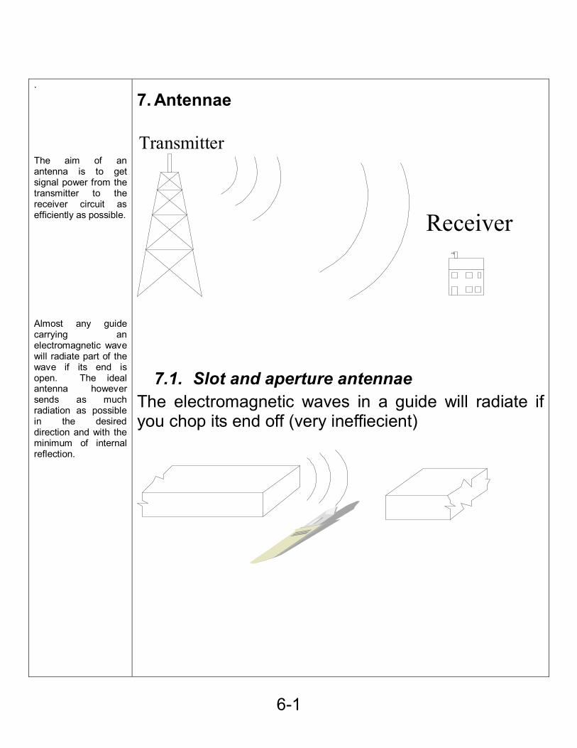
. The aim of an antenna is to get signal power from the transmitter to the receiver circuit as efficiently as possible. Almost any guide carrying an electromagnetic wave will radiate part of the wave if its end is open. The ideal antenna however sends as much radiation as possible in the desired direction and with the minimum of internal reflection.

7. Antennae Transmitter

Receiver

7.1. Slot and aperture antennae The electromagnetic waves in a guide will radiate if you chop its end off (very ineffiecient)

7-2

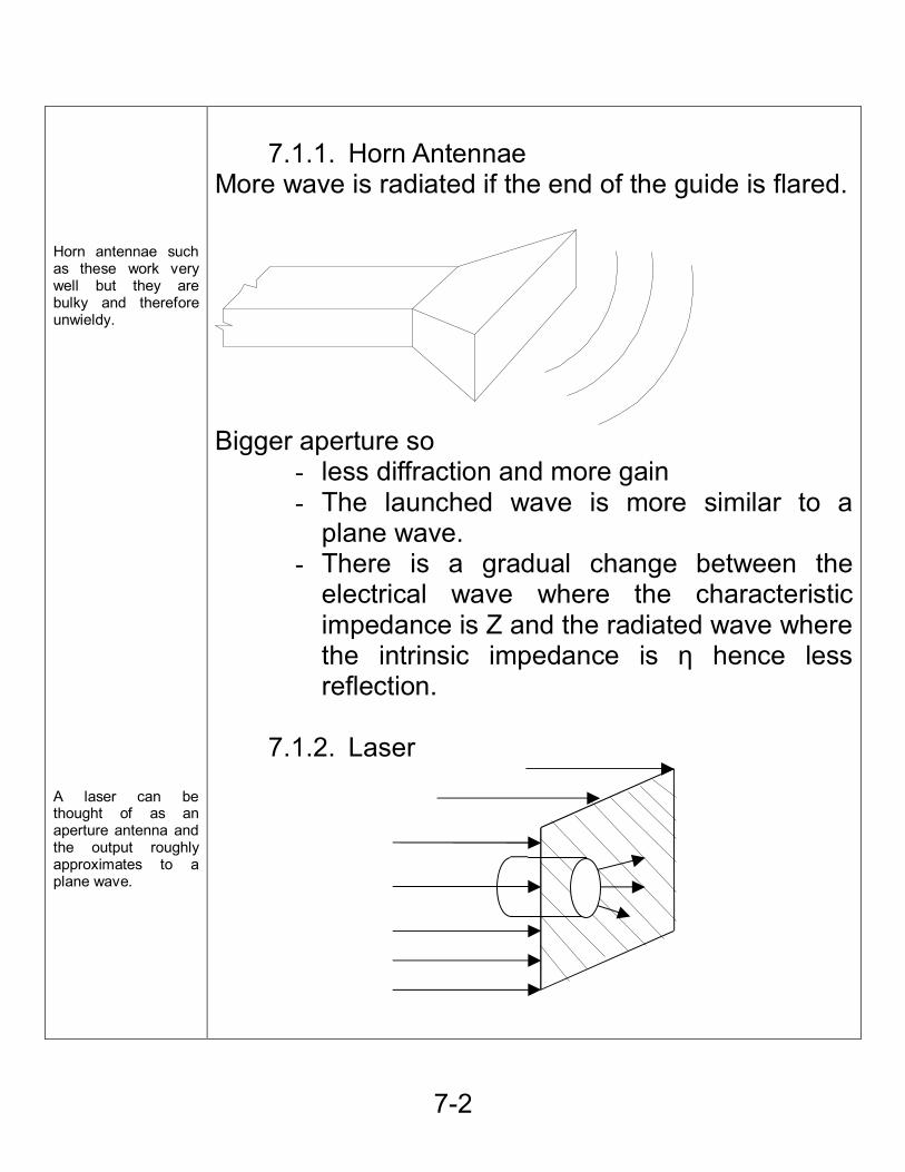
Horn antennae such as these work very well but they are bulky and therefore unwieldy. A laser can be thought of as an aperture antenna and the output roughly approximates to a plane wave.

7.1.1. Horn Antennae

More wave is radiated if the end of the guide is flared.

Bigger aperture so

- less diffraction and more gain - The launched wave is more similar to a

plane wave. - There is a gradual change between the

electrical wave where the characteristic impedance is Z and the radiated wave where the intrinsic impedance is η hence less reflection.

7.1.2. Laser

7-3

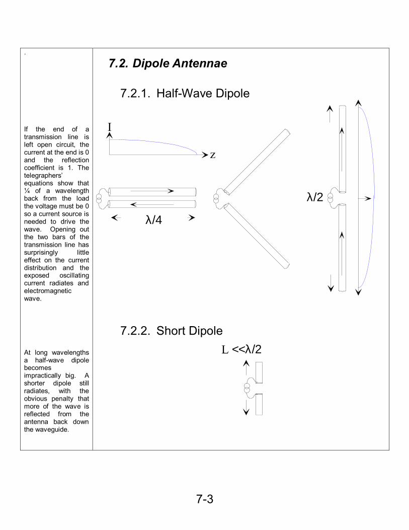
. If the end of a transmission line is left open circuit, the current at the end is 0 and the reflection coefficient is 1. The telegraphers’ equations show that ¼ of a wavelength back from the load the voltage must be 0 so a current source is needed to drive the wave. Opening out the two bars of the transmission line has surprisingly little effect on the current distribution and the exposed oscillating current radiates and electromagnetic wave. At long wavelengths a half-wave dipole becomes impractically big. A shorter dipole still radiates, with the obvious penalty that more of the wave is reflected from the antenna back down the waveguide.

7.2. Dipole Antennae

7.2.1. Half-Wave Dipole

λ/2

λ/4

I

z

7.2.2. Short Dipole L <<λ/2

7-4

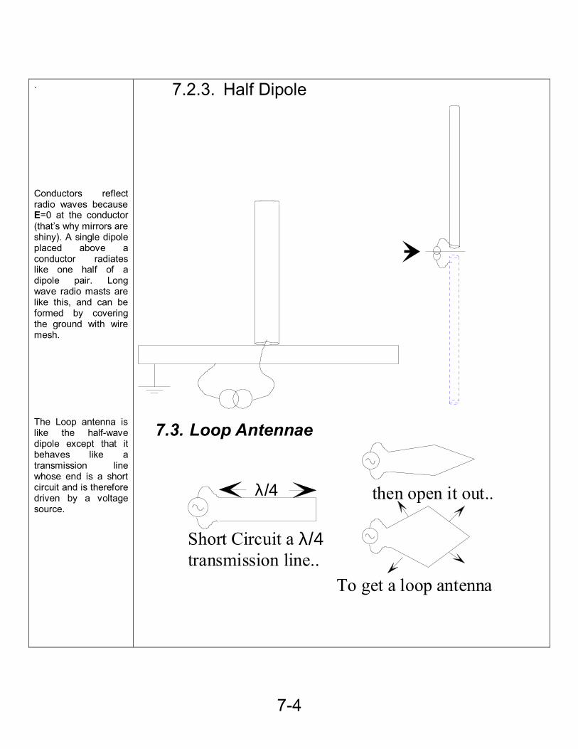
. Conductors reflect radio waves because E=0 at the conductor (that’s why mirrors are shiny). A single dipole placed above a conductor radiates like one half of a dipole pair. Long wave radio masts are like this, and can be formed by covering the ground with wire mesh. The Loop antenna is like the half-wave dipole except that it behaves like a transmission line whose end is a short circuit and is therefore driven by a voltage source.

7.2.3. Half Dipole

7.3. Loop Antennae

λ/4

Short Circuit a λ/4transmission line..

then open it out..

To get a loop antenna

7-5

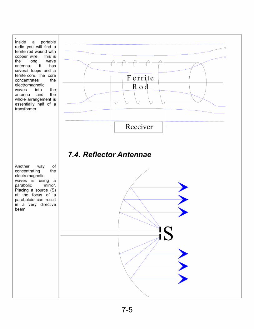
. Inside a portable radio you will find a ferrite rod wound with copper wire. This is the long wave antenna. It has several loops and a ferrite core. The core concentrates the electromagnetic waves into the antenna and the whole arrangement is essentially half of a transformer. Another way of concentrating the electromagnetic waves is using a parabolic mirror. Placing a source (S) at the focus of a parabaloid can result in a very directive beam

Receiver

F e r r i teR o d

7.4. Reflector Antennae

S

7-6

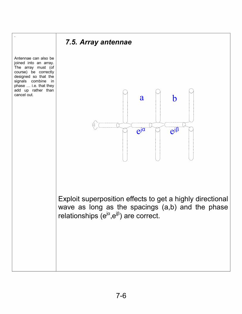
. Antennae can also be joined into an array. The array must (of course) be correctly designed so that the signals combine in phase … i.e. that they add up rather than cancel out.

7.5. Array antennae

a b

ejα ejβ

Exploit superposition effects to get a highly directional wave as long as the spacings (a,b) and the phase relationships (ejα,ejβ) are correct.

7-7

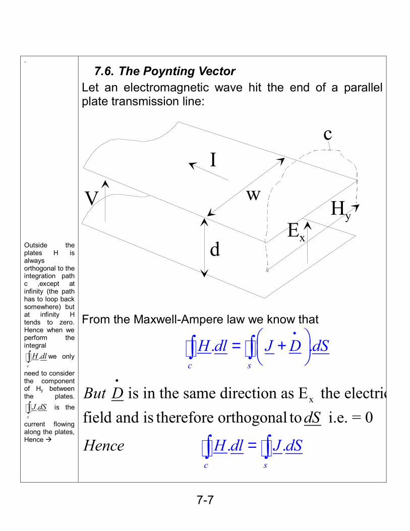
. Outside the plates H is always orthogonal to the integration path c ,except at infinity (the path has to loop back somewhere) but at infinity H tends to zero. Hence when we perform the integral

.c

H dl∫ we only

need to consider the component of Hy between the plates.

.s

J dS∫ is the

current flowing along the plates, Hence

7.6. The Poynting Vector Let an electromagnetic wave hit the end of a parallel plate transmission line:

V

I

dEx

Hy

c

w

From the Maxwell-Ampere law we know that

xis in the same direction as E the electricfield and is therefore orthog

. .

.

onal to i.e. =

.

0

c s

c s

H dl J D dS

H

But DdS

Hence dl J dS

•

• = +

=

∫ ∫

∫ ∫

7-8

The Poynting vector is defined to be the cross product, E x H. The complex Poynting vector is defined to be ½ E x H*.

Solving

.H w Iy =

Also the electric field and the voltage are related by:

.xE d V= So the transmission line wave power is:

* *1 12 2

x yV I E H wd=

The intensity of an electromagnetic wave

( )* 21 Re2

E H Wm−= ×

This expression is known as the complex Poynting Vector and the direction of power flow is perpendicular to E and H

7-9

.

7.6.1. Example – Duck a la microwave

A duck with a cross-sectional area of 0.1m2 is heated in a microwave oven. If the electromagnetic wave is:

( ) ( ) 1 1Re 750 , Re 2j t z j t zx yE e Vm H e Amω β ω β− −− −= =

What power is delivered to the duck ?

Power = ( )*1 .2E H Area×

=( )750 2 0.1× × = 75 W

.

8-1

. Where I is intensity … not current Actually impossible to make but useful as a definition !!

8. Radio

8.1. Radiation Resistance Antennae emit power, so they can be modelled as resistors: The radiation resistance, Ra, of an antenna is that resistance which in place of the antenna would dissipate as much power as the antenna radiates.

( )2

.antennas

a

I dSR

RMScurrent=

∫

8.2. Gain The gain(G) of an antenna is the factor by which its maximum radiated intensity exceeds that of an isotropic antenna if they emit equal power from an equal distance. G= Maximum value of I antenna at distance r Iisotropic at distance r Provided that . .antenna isotropic

s s

I dS I dS=∫ ∫

An Isotropic antenna is a hypothetical device which radiates equally in all directions

8-2

. The area of radio wave intercepted by a parabolic dish antenna is pretty obvious, but in principle a half wave dipole could have no area at all and yet still receive power from a radio wave. Hence we need to define an effective area.

8.3. Effective Area The effective area, Aeff , of an antenna is that area of wavefront whose power equals that received from the wavefront by the antenna. Aeff = Power collected by antenna Wave intensity (i.e. power/area) into antenna

8-3

8.4. Example – Power Transmission If two half-wave dipoles are 1 km apart and one is driven with 0.5 amps (RMS) at 300 MHz, what power is received by the other ? [ G = 1.64, Ra=73 Ω, Aeff=0.13 m2] Ans – Intensity r metres from an isotropic antenna = Transmitted power/(4πr2) Intensity r metres from this antenna

2

24ai RGrπ

=

Power received by receiving antenna = Intensity x Aeff

2

24a

effi RG Arπ

=

( )

2

20.5 731.64 0.13

4 1000π×= × ×

=0.3 µW