Possibilities of using thermal mass in buildings to save energy, cut power consumption peaks and increase the thermal comfort

Jonathan Karlsson

LUND INSTITUTE OF TECHNOLOGY LUND UNIVERSITY

Division of Building Materials

Report TVBM-3164 Licentiate thesis Lund 2012

ISRN LUTVDG/TVBM--12/3164--SE(1-100) ISSN 0348-7911 TVBM Lund Institute of Technology Telephone: 46-46-2227415 Division of Building Materials Telefax: 46-46-2224427 Box 118 SE-221 00 Lund, Sweden www.byggnadsmaterial.lth.se

i

PREFACE This licentiate thesis is a result of two years of research at Building Materials LTH at Lund University. The project was funded by three projects: a Cerbof project “Energibesparing genom utnyttjande av tunga byggnaders termiska beteende”, an Interreg project “Integrering mellem baeredyktige byggeprocesser”, and an IQS-project “Brukarkrav”. My main collaborators outside LTH have been Cementa AB, SP (Technical Research Institute of Sweden) and Luleå Technical University.

I would like to give special thanks to my supervisors Professor Lars Wadsö and adjunct Professor Mats Öberg at Building Materials, for their helpfulness and support for this research. Thanks also to Guest Professor Ronny Andersson at Structural Engineering, and the representatives from the industry, for their inspiration and driving force of the research. Also thanks to Carl-Erik Magnusson lecturer at the Physics department, Lund University, for his interest in my work.

The work during these years has been performed in corporation with the technical staff at Building Materials, Bo Johansson, Stefan Backe and Bengt Nilsson, which with their experience have simplified the laboratory works. The administrative personel Marita Persson, Britt Andersson and Helena Klein have also been helpful with their administration experiences.

Further, would like to thank all my colleagues at the Building Material department for their advice and support.

Finally, I want to express my appreciation to my life partner Caroline and my family, especially my father, for their support and helpfulness.

ii

iii

ABSTRACT The aim of this project was to generate knowledge to enable us to take advantage of heat storage in heavy building structures with regard to as energy savings, better thermal indoor climate, and reduced peak powers. This could include buildings that can function without energy input during cold periods, buildings that give a robust indoor climate without installed cooling, and buildings with good thermal comfort also in case of higher outdoor temperatures resulting from global warming. To reach this aim, calculation models that take thermal mass into account have been developed and investigated and the thermal properties of concrete – the most common thermally heavy building material – have been explored. Reduced peak powers is probably the most important advantage in the future as it can give both environmental effects (less peak power needed) and reduce the size of the energy supply systems (both at the energy supplier and at each building).

KEY WORDS Energy storage, time constant, thermal mass, thermal inertia, thermal properties, thermal conductivity, heat capacity, concrete, aggregates.

iv

SAMMANFATTNING Detta projekt syftade till att generera ny kunskap som gör det möjligt för oss att dra nytta av de möjligheter som skapas av värmelagring i tunga stommar och material i byggnaden med avseende på energibesparing, lägre effektbehov och ett bättre termiskt inneklimat. Detta kan t ex gälla byggnader med hög värmelagringsförmåga som klarar kalla perioder utan tillförsel av energi, byggnader med stabil inomhustemperatur utan kylning, och byggnader med ett gott inomhusklimat även med ökande uttetemperaturer från global uppvärmning. För att uppnå detta mål har vi utvecklat modeller för byggnader med hög termisk massa samt undersökt de termiska egenskaperna hos betong – det material som ger högst termisk massa i byggnader. Av fördelarna med termiskt tunga material är troligtvis sänkt effektbehov den mest betydelsefulla i framtiden eftersom den kan ge både miljömässiga fördelar (minskad topproduktion) och reducera energidistributions-systemens storlek (både hos energileverentören och i varje byggnad).

v

PAPERS

PAPER I E.-L. W. Kurkinen and J. Karlsson “Different materials with high thermal mass and its influence on a building’s heat loss – an analysis based on the theory of dynamic thermal networks”, Proceedings of the 5th International Building Physics Conference (IBPC), 28-31 May 2012, Kyoto University, Japan (accepted).

Paper II J. Karlsson, L. Wadsö and M. Öberg “A conceptual model that simulates the influence of thermal inertia in building structures” (submitted to Energy and Buildings)

PAPERIIIL. Wadsö, J. Karlsson and K. Tammo “Thermal properties of concrete with various aggregates” (submitted to Cement and Concrete Research)

vi

vii

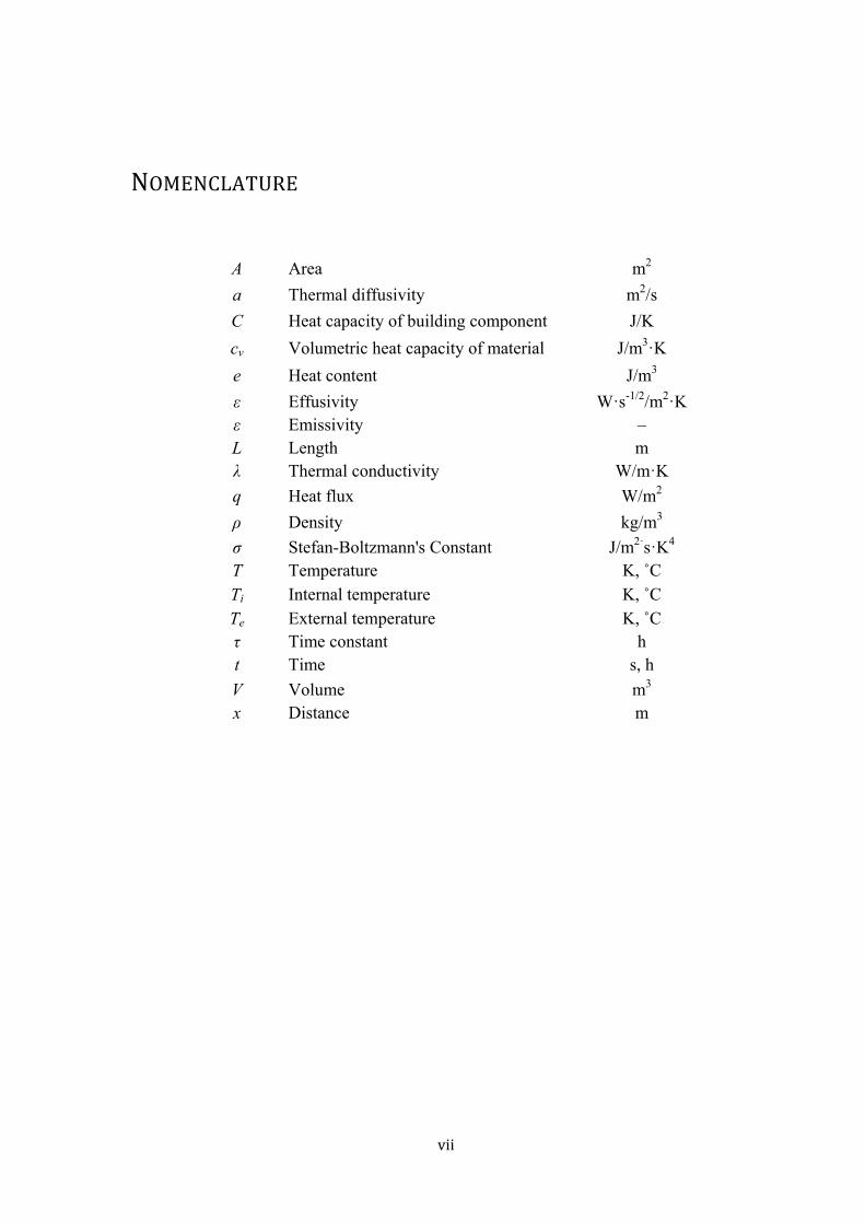
NOMENCLATURE

A Area m2

a Thermal diffusivity m2/s

C Heat capacity of building component J/K

cv Volumetric heat capacity of material J/m3·K

e Heat content J/m3

ε Effusivity W·s-1/2/m2·K ε Emissivity – L Length m λ Thermal conductivity W/m·K

q Heat flux W/m2

ρ Density kg/m3

σ Stefan-Boltzmann's Constant J/m2·s·K4 T Temperature K, ˚C Ti Internal temperature K, ˚C Te External temperature K, ˚C τ Time constant h t Time s, h

V Volume m3 x Distance m

viii

ix

CONTENTS

1 INTRODUCTION

1.1 Background 1.2 Objective 1.3 Limitations

2 THEORETICAL BACKGROUND

2.1 Steady state heat conduction 2.2 Heat capacity 2.3 Heat balance 2.4 Diffusivity and effusivity 2.5 Convection 2.6 Radiation 2.7 The thermal time constant 2.8 One to three dimensional heat conduction

3 METHODS AND MATERIALS

3.1 Heat storage measurement 3.2 Thermal property measurements on concretes 3.3 Simulation model for the influence of thermal inertia 3.4 An example of active heat storage 3.5 Simulation in VIP energy

4 RESULTS

4.1 Heat storage measurement 4.2 Thermal property measurements on concretes 4.3 Simulation model for the influence of thermal inertia 4.4 An example of active heat storage 4.5 Simulation in VIP energy

5 DISCUSSION

6 REFERENCES

APPENDIX

PAPERS

x

1

1 INTRODUCTION

1.1BACKGROUND

The building sector needs to become more energy efficient. Traditional ways to reduce energy consumption in buildings are to increase the insulation (reducing conductive heat losses), make buildings more air-tight and reduce ventilation losses by heat recovery. Another aspect to consider is the user behaviour, which may cause substantial differences in energy use; therefore, savings can also be achieved through information.

New systems for indoor air conditioning have been developed and introduced. This has contributed to greater comfort, but at the same time also to a more expensive operation, e.g., it is common that different parts of buildings are heated and cooled at the same, which is not energy efficient. This is caused by such factors as individual temperature regulation in different rooms, and high heat production from office machines.

To move forward we need to utilize the laws of nature in the design of buildings and in the operation of installations and allow the buildings themselves to assist with temperature control; use the building dynamics to our advantage.

One way to do this is to use the heat capacity of massive buildings in useful ways. Typically, a heavy building can have a three times higher time constant (cf. Eq. 4 below) than a light building, so a heavy building will cool down or heat up three times slower, all other factors the same. As a lightweight building reacts more quickly to external temperature changes, the heating system must be dimensioned for a single day (or those hours) with the lowest outdoor temperatures, while a heavy building can keep its internal temperature within reasonable limits during a day or two without heating or cooling.

The thermal mass of buildings has been recognized as being important by many researchers. For example did Al-Sanea and Zedan (2012) and Al-Temeeni et al. (2004) investigate the positive aspects of high thermal mass in hot climates; Bloomsfield and Fisk (1977) and Pupeikis and Burlingis (2010) studied intermittent heating for which the thermal mass is an important factor; Balaras (1996) and Yang and Li (2008) looked at cooling loads of buildings; Yam and Li (2003) and Zhou and Zhang (2008) studied the coupling between thermal mass and ventilation. Li and Xu (2006) discussed the general merits of thermally heavy buildings in a paper called “Thermal mass design in buildings – heavy or light?” and presented a simple design method to determine the thermal mass of a building. Few experimental studies have been made in which the properties of thermally heavy and light buildings have been compared. An interesting study is Bellamy and Mackenzie (2001) that investigated two test houses that were similar in all respects except for their thermal mass.

Thermal storage is an important factor in many technical and scientific applications as heat is often available at times when it is not needed. By storing excess energy, it can be used later when there is a need for it. This has become even more interesting today with

2

the development of devices to collect renewable energy, such as solar collectors, wind turbines and wave turbines. Note that also the renewable energy ‘sources’ that produce electricity can benefit from heat storage; for example can electricity from wind power be used to cool an office building during the night, to prevent over-temperatures during the following day. Also note that when terms such as “storage of heat” are used in a general way, they also include the storage of “coldness”. Most storage principles are reversible and can be used both to store heat and “coldness”, although it is in both cases the heat that is transported.

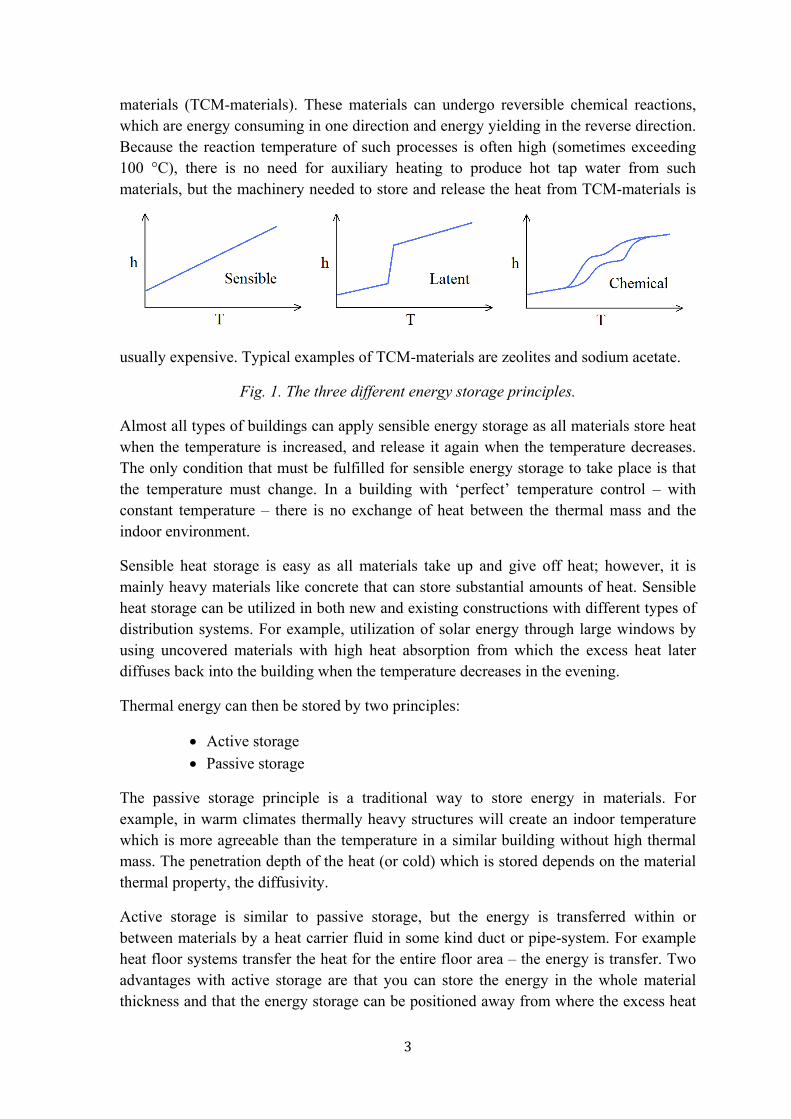
Thermal energy storage can be of three types (Fig. 1):

Sensible – storage based on heat capacity.

Latent – storage based on phase change.

Chemical – storage based on chemical processes.

In sensible heat storage the temperature is gradually changing as the medium is charged or discharged with heat. The amount of heat that gives a certain temperature change for a certain material is called the heat capacity, and materials with higher heat capacity can store more heat. It is desirable for a storage medium for sensible heat to have a high volumetric heat capacity and also not too low heat conductivity. A current technology is storage of heat in warm water – water has a high volumetric heat capacity – by using either water accumulators or underground natural buffers, also called aquifers. These underground natural buffers consist of geologically determined water conducting sand layers at a depth of about 100 m, the top and bottom of which are impermeable to water. As these storages are large, they can be used to store heat over longer periods of time, also called seasonal storage. Storage for short time intervals, also called daily storage, is in smaller water accumulators or in solid materials suitable for sensible heat storage such as heavy building materials. For instance will a concrete with magnetite aggregate have a higher heat storage potential than normal concrete (discussed below).

In latent heat storage the storage material changes its phase, normally from liquid to solid and vice versa. It does, for example, require a large amount of energy to melt ice, and ice can thus be used as a store for coldness in cooling applications. In relation to sensible heat storage a lower mass and volume is needed to store the same amount of energy by latent heat storage. It thus provides high density energy storage and has the capacity to store latent heat at different temperatures (as long as one does not pass the phase change temperature). For instance, it requires about 4.18 kJ to raise one kilogram of water by one degree, while a kilogram of ice requires about 330 kJ to melt. It is a factor of about 80 between these values. A modern material for phase change applications is pellets of paraffin that can be manufactured to have different melting points adapted for different purpose. Such materials are called Phase Change Materials (PCM) and they can be incorporated into building materials; for example gypsum boards with paraffin PCM.

An additional principle of long term storage of thermal energy, without the necessity for thermal insulation, is by means of chemical energy in so-called thermo chemical

3

materials (TCM-materials). These materials can undergo reversible chemical reactions, which are energy consuming in one direction and energy yielding in the reverse direction. Because the reaction temperature of such processes is often high (sometimes exceeding 100 °C), there is no need for auxiliary heating to produce hot tap water from such materials, but the machinery needed to store and release the heat from TCM-materials is

usually expensive. Typical examples of TCM-materials are zeolites and sodium acetate.

Fig. 1. The three different energy storage principles.

Almost all types of buildings can apply sensible energy storage as all materials store heat when the temperature is increased, and release it again when the temperature decreases. The only condition that must be fulfilled for sensible energy storage to take place is that the temperature must change. In a building with ‘perfect’ temperature control – with constant temperature – there is no exchange of heat between the thermal mass and the indoor environment.

Sensible heat storage is easy as all materials take up and give off heat; however, it is mainly heavy materials like concrete that can store substantial amounts of heat. Sensible heat storage can be utilized in both new and existing constructions with different types of distribution systems. For example, utilization of solar energy through large windows by using uncovered materials with high heat absorption from which the excess heat later diffuses back into the building when the temperature decreases in the evening.

Thermal energy can then be stored by two principles:

Active storage

Passive storage

The passive storage principle is a traditional way to store energy in materials. For example, in warm climates thermally heavy structures will create an indoor temperature which is more agreeable than the temperature in a similar building without high thermal mass. The penetration depth of the heat (or cold) which is stored depends on the material thermal property, the diffusivity.

Active storage is similar to passive storage, but the energy is transferred within or between materials by a heat carrier fluid in some kind duct or pipe-system. For example heat floor systems transfer the heat for the entire floor area – the energy is transfer. Two advantages with active storage are that you can store the energy in the whole material thickness and that the energy storage can be positioned away from where the excess heat

4

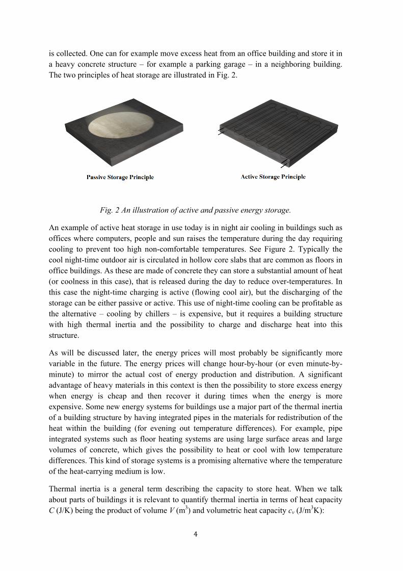
is collected. One can for example move excess heat from an office building and store it in a heavy concrete structure – for example a parking garage – in a neighboring building. The two principles of heat storage are illustrated in Fig. 2.

Fig. 2 An illustration of active and passive energy storage.

An example of active heat storage in use today is in night air cooling in buildings such as offices where computers, people and sun raises the temperature during the day requiring cooling to prevent too high non-comfortable temperatures. See Figure 2. Typically the cool night-time outdoor air is circulated in hollow core slabs that are common as floors in office buildings. As these are made of concrete they can store a substantial amount of heat (or coolness in this case), that is released during the day to reduce over-temperatures. In this case the night-time charging is active (flowing cool air), but the discharging of the storage can be either passive or active. This use of night-time cooling can be profitable as the alternative – cooling by chillers – is expensive, but it requires a building structure with high thermal inertia and the possibility to charge and discharge heat into this structure.

As will be discussed later, the energy prices will most probably be significantly more variable in the future. The energy prices will change hour-by-hour (or even minute-by-minute) to mirror the actual cost of energy production and distribution. A significant advantage of heavy materials in this context is then the possibility to store excess energy when energy is cheap and then recover it during times when the energy is more expensive. Some new energy systems for buildings use a major part of the thermal inertia of a building structure by having integrated pipes in the materials for redistribution of the heat within the building (for evening out temperature differences). For example, pipe integrated systems such as floor heating systems are using large surface areas and large volumes of concrete, which gives the possibility to heat or cool with low temperature differences. This kind of storage systems is a promising alternative where the temperature of the heat-carrying medium is low.

Thermal inertia is a general term describing the capacity to store heat. When we talk about parts of buildings it is relevant to quantify thermal inertia in terms of heat capacity C (J/K) being the product of volume V (m3) and volumetric heat capacity cv (J/m3K):

5

vcVC (1)

The higher the heat capacity is, the higher is the thermal inertia. Looking at a building composed of different parts made of different materials, the total heat capacity is the sum of the individual heat capacities of the individual materials:

i

n

iCC

1 (2)

The heat loss rate from a building can be quantified as an overall heat transfer coefficient k (W/K) that relates the heat loss rate q (W) to the difference between the internal (indoor) temperature Ti (K) and the external (outdoor) temperature Te (K):

)( ei TTkq (3)

Here, the overall heat transfer coefficient includes heat losses through the thermal envelope and losses through the ventilation. From the heat transfer coefficient and the

heat capacity a time constant (s) can be calculated as:

k

C (4)

Lumped whole-building thermal parameters like the building time constants have been discussed, e.g., by Antonopoulous and Tzivanidis (1996) and Fernández and Porta-Gándara (2005).

If a cold spell impacts a building envelope it will gradually cause a temperature decrease of the entire building (if the building is not heated), and the rate at which this cooling takes place is determined by the time constant of the building. The time constant is therefore a relevant measure of the thermal inertia of a building. The time constant τ is a measure of how rapidly a temperature change occurs according to an exponential decay function. If the external temperature is changed step-wise, the internal temperature will

after 0.1, 0.2, 0.3, 0.5 and 1.0 have changed 10%, 18%, 26%, 39% and 63% of the final temperature change. For a building this can be measured by turning off the heating power on a cold day to see how quickly the internal temperature drops. For a heavy building, the time constant can be 300 hours, while the time constant of a light building (with the same thermal conductivity of the thermal envelope) can be less than 100 hours. The time constant is important for the power demand both in winter when cold spells occur and during hot days in the summer. The time constant is also important for the sensitivity to disruptions of the energy production, for example during a power failure.

Note that high thermal inertia of a building – as defined through the building time constant – is achieved by a combination of a high heat capacity and a low overall heat transfer coefficient. A prerequisite for high thermal inertia is therefore a heavily insulated structure with an energy efficient ventilation system (including a tight envelope and heat recovery); those parameters that earlier in the introduction were mentioned as the most

6

two important factors for buildings with low heat consumption. It is thus natural to see a development of energy efficient buildings in stages that build on each other: good insulation, tight envelope, controlled ventilation, heat recovery, and – as is discussed here – high thermal inertia.

The time constant of a building should be seen as a simplified, overall parameter approximately describing the thermal inertia of a building. It is for example dependent on the availability of the heat capacities in a building; cf. underlying joists and other heat capacities that are not placed fully inside the thermal envelope, Also, during rapid temperature changes the heat only the surface part of a material can be utilized for energy storage. However, time constants determined by shutting down the energy system during a certain time to measure the temperature decrease are still a good way to determine the thermal time constant of a whole while building.

An effective thermal storage has to be adjusted to the application and also to the surrounding environment, as thermal mass can also be negative. For example will high thermal inertia increase the heat consumption of an intermittently heated building, e.g., a week-end cabin. Therefore it is needed to be innovative and try to design buildings in the most optimal way. As an example, the temperature in Sweden is rather low during the cold season, and the sun can be a valuable source of free heat. Many low-energy houses utilize solar radiation by large south-facing windows, but this has in many cases resulted in significant over-temperatures, at least partly because most low-energy buildings are light structures with low heat capacity. However, in a thermally heavy building it may be possible to have large windows to the south, but to have the sun shine on floors and walls made of thermally heavy materials, for example the concrete with magnetite aggregate (discussed in paper III).

1.2 OBJECTIVES

The objectives of this work were to:

Investigate the thermal properties of concretes with unusual aggregates.

Investigate how material properties of thermally heavy construction materials influence the thermal properties of a building.

Create a simple tool that makes it easy to investigate and visualize the effects of high thermal inertia in buildings.

1.3LIMITATIONS

This thesis primarily investigates passive energy storage, and is focused on how the thermal properties of materials will influence the following three factors:

Energy consumption

Power needs

Thermal comfort

7

2 PHYSICAL BACKGROUND This chapter deals with heat transfer mechanisms, numerical solutions of heat transfer problems, and the concept of thermal time constant.

The transport or flow of energy in the form of heat is generally termed ‘heat transfer’. Heat transfer will continue as long as there is a temperature difference in the medium (or between two media) and ends when the system has reached thermal equilibrium. Heat can be transferred in three different modes:

Conduction

Convection

Radiation They all require the existence of temperature differences.

2.1STEADYSTATEHEATCONDUCTION

Conduction is the transfer of energy from more energetic molecules of matter to less energetic ones as a result of interactions between the molecules. It takes place in solids, liquids and gases. Conduction in solids is due to a combination of the molecular lattice vibrations and the energy transport by free electrons. In gases and liquids it is due to the collisions and diffusion of the molecules during their random motion.

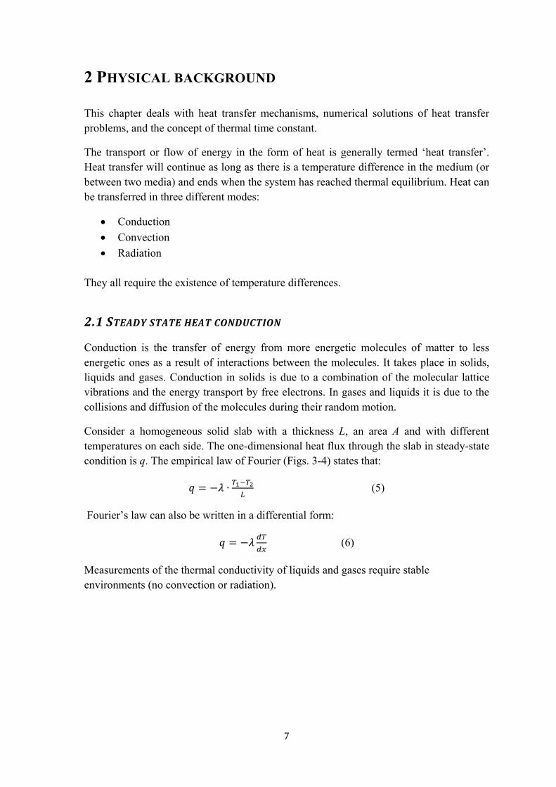
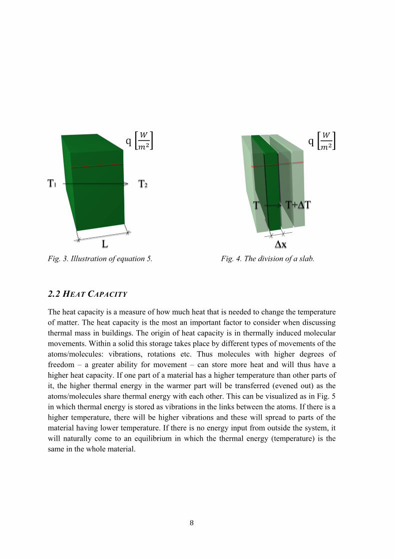
Consider a homogeneous solid slab with a thickness L, an area A and with different temperatures on each side. The one-dimensional heat flux through the slab in steady-state condition is q. The empirical law of Fourier (Figs. 3-4) states that:

∙ (5)

Fourier’s law can also be written in a differential form:

(6)

Measurements of the thermal conductivity of liquids and gases require stable environments (no convection or radiation).

8

Fig. 3. Illustration of equation 5. Fig. 4. The division of a slab.

2.2 HEAT CAPACITY

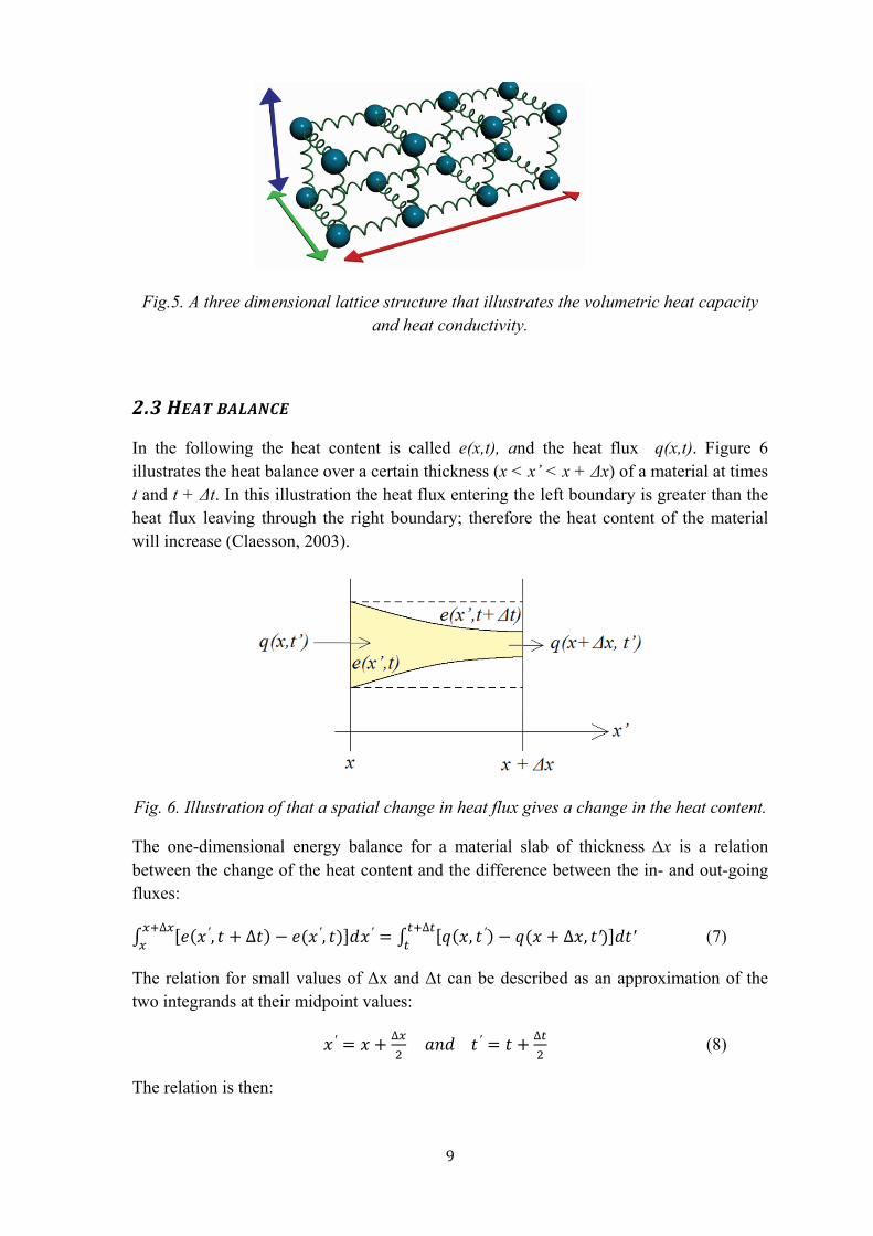
The heat capacity is a measure of how much heat that is needed to change the temperature of matter. The heat capacity is the most an important factor to consider when discussing thermal mass in buildings. The origin of heat capacity is in thermally induced molecular movements. Within a solid this storage takes place by different types of movements of the atoms/molecules: vibrations, rotations etc. Thus molecules with higher degrees of freedom – a greater ability for movement – can store more heat and will thus have a higher heat capacity. If one part of a material has a higher temperature than other parts of it, the higher thermal energy in the warmer part will be transferred (evened out) as the atoms/molecules share thermal energy with each other. This can be visualized as in Fig. 5 in which thermal energy is stored as vibrations in the links between the atoms. If there is a higher temperature, there will be higher vibrations and these will spread to parts of the material having lower temperature. If there is no energy input from outside the system, it will naturally come to an equilibrium in which the thermal energy (temperature) is the same in the whole material.

9

Fig.5. A three dimensional lattice structure that illustrates the volumetric heat capacity and heat conductivity.

2.3HEATBALANCE

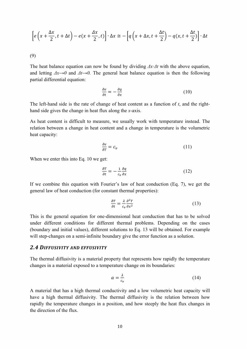
In the following the heat content is called e(x,t), and the heat flux q(x,t). Figure 6 illustrates the heat balance over a certain thickness (x < x’ < x + Δx) of a material at times t and t + Δt. In this illustration the heat flux entering the left boundary is greater than the heat flux leaving through the right boundary; therefore the heat content of the material will increase (Claesson, 2003).

Fig. 6. Illustration of that a spatial change in heat flux gives a change in the heat content.

The one-dimensional energy balance for a material slab of thickness x is a relation between the change of the heat content and the difference between the in- and out-going fluxes:

′, ∆ ′, ′ , ′ ∆ , ′ ′∆∆

(7)

The relation for small values of Δx and Δt can be described as an approximation of the two integrands at their midpoint values:

′ ∆ ′ ∆ (8)

The relation is then:

10

∆2, ∆

2, ∙ ∆ ≅ ∆ ,

∆2

,∆2

∙ ∆

(9)

The heat balance equation can now be found by dividing Δx·Δt with the above equation, and letting Δx→0 and Δt→0. The general heat balance equation is then the following partial differential equation:

(10)

The left-hand side is the rate of change of heat content as a function of t, and the right-hand side gives the change in heat flux along the x-axis.

As heat content is difficult to measure, we usually work with temperature instead. The relation between a change in heat content and a change in temperature is the volumetric heat capacity:

(11)

When we enter this into Eq. 10 we get:

(12)

If we combine this equation with Fourier’s law of heat conduction (Eq. 7), we get the general law of heat conduction (for constant thermal properties):

(13)

This is the general equation for one-dimensional heat conduction that has to be solved under different conditions for different thermal problems. Depending on the cases (boundary and initial values), different solutions to Eq. 13 will be obtained. For example will step-changes on a semi-infinite boundary give the error function as a solution.

2.4DIFFUSIVITYANDEFFUSIVITY

The thermal diffusivity is a material property that represents how rapidly the temperature changes in a material exposed to a temperature change on its boundaries:

(14)

A material that has a high thermal conductivity and a low volumetric heat capacity will have a high thermal diffusivity. The thermal diffusivity is the relation between how rapidly the temperature changes in a position, and how steeply the heat flux changes in the direction of the flux.

11

An important factor in connection to sensible energy storage is the effective thickness of a material that can be used for energy storage on a certain time scale. This can be quantified in terms of a penetration depth x which is dependent to the thermal diffusivity of the material:

atd (15)

The penetration depth is the position in a material into which about 50% of a temperature change at the surface has penetrated.

The thermal effusivity has the definition:

(16)

The effusivity can be seen as a measure of how easily a material exchanges heat with its surroundings. The temperature at the interface between two materials that are placed in contact with each other is for example governed by the effusivities of the two materials. If you place your hand on steel or wood, you feel that steel is colder than wood, because heat is transferred from your hand to the steel at a higher rate because steel has a higher thermal effusivity than wood.

2.5 CONVECTION

Thermal convection is when heat is carried by a moving fluid (gas or liquid). This does not take place in materials – except in large pores at high temperature gradients – but is important in fluids in contact with materials at their boundaries. There are two types of convection: natural convection driven by density differences and forced convection driven by external forces.

Consider a gas volume bounded by two walls with different temperatures. If the temperature on wall 2 is higher than the temperature on wall 1, the gas close to wall 2 will be heated, decrease its density, and therefore have a tendency to rise. The gas at wall 1 will instead be cooled and have a tendency to drop. These tendencies to rise and drop will give rise to a circulating gas movement which will transport heat from the warmer to the colder wall more efficiently than only heat conduction. This is called natural convection as the fluid motion is caused by buoyancy forces that are induced by density differences due to the variation of temperature in the fluid. On the other hand, forced convection is when the fluid is forced to flow over the surface by external means such as a fan, pump, or the wind.

The rate of convective heat transfer at a surface by forced convection is generally expressed as:

∞ (17)

Where h is the convective heat transfer coefficient in W/m2K, TS is the surface temperature, and ∞ is the temperature of the fluid sufficiently far from the surface.

12

2.6RADIATION

A body with a thermodynamic temperature of more than zero kelvins emits electromagnetic radiation at certain wavelengths and in all directions. This occurs as a result of the change in motion of atoms and molecules. The wavelength of this electromagnetic radiation depends on the temperature of the emitting body. The radiation is of the same nature as light and has the same propagation speed as light, though we call it thermal radiation or infra-red radiation when its wavelength is longer than that of visible light. Thermal radiation has the wavelength range between 10-7 – 10-4 m, i.e., it acts in the infrared spectral range, whereas visible light can be found in the interval 3,9·10-7 – 7,8·10-7 m. The thermal radiation maximum is shifted to shorter wavelength when the surface temperature increases.

The radiation causes a net flow of energy from a warmer to a colder body. Different bodies absorb and emit different amounts of energy per unit surface area, even when they are the same circumstances, which mean that all materials have a specific absorption and emission factors. Absorption refers to the ability to absorb radiation. Emissivity refers to the ability to emit radiation. A determination of these parameters requires the definition of an idealized body, called black body.

The connection between the exchanges on a surface can be described by three parameters: absorption a, reflection r and transmission t, which are related as:

1 (18)

A black body absorbs all incident radiation. The radiation energy emitted by a black body is:

(19)

This is the Stefan-Boltzmann law, where 5.67 ∙ 10 W m-2K-4 is the Stefan-Boltzmann constant and T is the absolute temperature of the surface. The radiation emitted by all real surfaces is less than the radiation emitted by a black body at the same temperature as:

(20)

Here ε is the emissivity of the surface. Emissivity has values in the range of 0 1, and is a measure of how closely a surface approximates a black body for which ε=1.

The net heat radiation that reaches the surface A1,that exchanges radiation with a much larger surface A2 (A1<<A2) is:

(21)

Between two parallel surfaces this equation becomes:

(22)

13

Where 12 is defined by

1. (23)

2.7THETHERMALTIMECONSTANT

As discussed in the introduction, the thermal inertia of a building can be quantified by its

thermal time constant that describes how long it takes for the temperature of the building to change if the heating/cooling of the building is discontinued. The thermal time constant is defined as the ratio of a building’s thermal mass and its overall heat loss coefficient. Both the thermal masses and the overall heat losses are difficult parameters to define in an exact sense, but the following approximate relation is useful:

∑ ∙

∑ (24)

Here, cvV is the sum of all the heat capacities inside the thermal envelope (volumetric

heat capacity of each material times its volume), and k is the sum of all thermal conductances between the interior and the exterior of the building. The time constant can be used in a model of how the temperature inside a building changes if, e.g., the heating of a building is discontinued in the winter. The temperature change is then described by an exponential function:

∆ ∆ ∙ / (25)

Here, T0 is the temperature difference at time zero, and Tt is the interior temperature at a time t after the heating was discontinued. The time constant may in principle be determined either by performing measurements on buildings or by calculating it, based on construction design data.

The single time constant description has its limitation, as it assumes that all parts of a building inside the thermal envelope have the same temperature. Rapid temperature changes will only affect the surface layer of materials, while slow changes will influence the whole mass of even heavy structures, and thus give a greater thermal storage. However, if we discuss temperature changes that takes place during comparatively long time periods, e.g., days, all materials inside the thermal envelope will have approximately the same temperature. Another limitation with the single time constant is that it does not – as it is defined in Eq. 24 – include, e.g., ventilation heat losses, but an approximate

adjustment of can be made to include such effects.

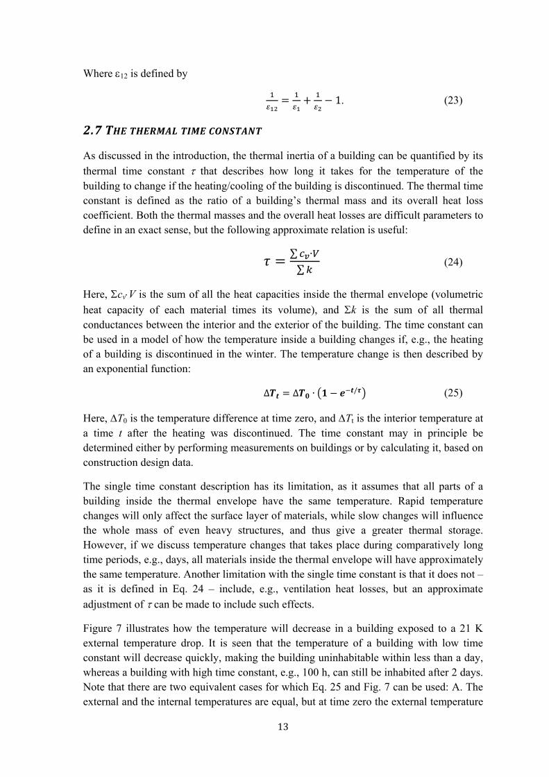
Figure 7 illustrates how the temperature will decrease in a building exposed to a 21 K external temperature drop. It is seen that the temperature of a building with low time constant will decrease quickly, making the building uninhabitable within less than a day, whereas a building with high time constant, e.g., 100 h, can still be inhabited after 2 days. Note that there are two equivalent cases for which Eq. 25 and Fig. 7 can be used: A. The external and the internal temperatures are equal, but at time zero the external temperature

14

is decreased. B. The external temperature is low and the building is heated until time zero when the heating is turned off. Case B is more realistic for a building in a cold climate, but this type of problems is often formulated mathematically like case A.

Fig. 7. The temperatures decrease of different buildings with different time constants

(given in the figure) when the external temperature is 0 C and the heating is turned off at

time zero (when the indoor temperature was 21 C).

The following reformulation of Eq. 25 can be used to calculate the time at which the temperature of a building has decreased to Ti after a shut-off of the heating:

∙,

(26)

Where Ti is the temperature at time t, Ti,0 the initial indoor temperature and Te the external temperature.

2.8NUMERICALSOLUTIONS

Numerical solutions to the general heat conduction equation can be made in different ways. The simplest way – and the way that most resembles the physical situation – is to by dividing a sample into small cells and repeatedly apply Fourier’s law of heat conduction (Eq. 7) and the heat balance equation (Eq. 12). This is called the explicit forward difference method as Eqs. 7 and 12 are used without any reformulations (other methods – implicite forward differences or the finite element method (FEM) – uses more refined mathematical formulations). In a one-dimensional formulation the cells are arranged adjacent to each other as a vector through the medium with a separation distance Δx.

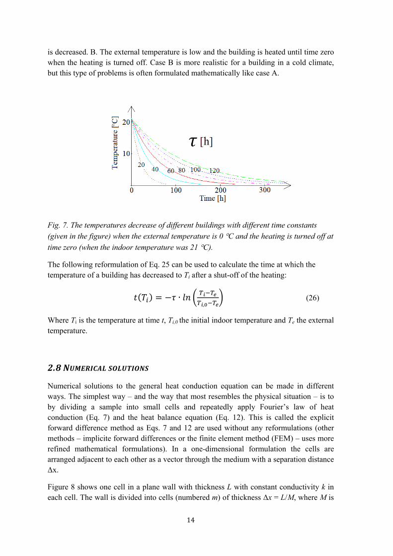
Figure 8 shows one cell in a plane wall with thickness L with constant conductivity k in each cell. The wall is divided into cells (numbered m) of thickness Δx = L/M, where M is

15

the total number of cells. The coordinates in the x-direction of the center of a cell m is xm

= (m-0.5)Δx. Each cell is assumed to have a constant temperature T(xm) = Tm (can be seen as the temperature at each point). The calculation approximation is better the smaller the distance Δx is between two cells.

Fig. 8. One dimensional steady state heat conduction.

When appropriate start and boundary conditions have been applied, the simulation proceeds by repeating two steps. In each step of the calculations one will first calculate all heat flows between cells (Fourier’s law) and then calculate the resulting temperature changes (with the heat balance equation). The method is easily reformulated in two and three dimensions, by using cells with surface or volume cells. This is the method used in paper II to simulate how the thermal properties of an interior concrete wall influence energy consumption and other factors.

Another way to numerically investigate the influence of thermal mass on, e.g., energy consumption is to use a Discrete Thermal Network (DTN) model. This can be seen as a dynamic counterpart to the stationary U-values that are normally used to quantify the thermal properties of building components. In a DTN model each building component is quantified by functions, not single numbers. To model the dynamic behavior, more information is needed than for the stationary case where a single number, such as the U-value, is sufficient to understand the behavior. The DTN-theory is described in paper I and in Claesson (2003).

16

17

3 METHODS AND MATERIALS

Investigation of the energy storage in building materials and building structures were made by laboratory experiments and calculations. This chapter is divided into the following sections: - Heat storage measurements

Passive thermal storage Active thermal storage

- Thermal property measurements of concretes with different aggregates - A conceptual model that simulates the influence of thermal inertia in building structures

3.1 HEAT STORAGE MEASUREMENTS - PASSIVE STORAGE

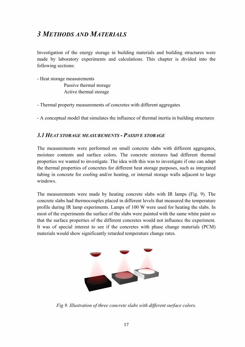
The measurements were performed on small concrete slabs with different aggregates, moisture contents and surface colors. The concrete mixtures had different thermal properties we wanted to investigate. The idea with this was to investigate if one can adapt the thermal properties of concretes for different heat storage purposes, such as integrated tubing in concrete for cooling and/or heating, or internal storage walls adjacent to large windows. The measurements were made by heating concrete slabs with IR lamps (Fig. 9). The concrete slabs had thermocouples placed in different levels that measured the temperature profile during IR lamp experiments. Lamps of 100 W were used for heating the slabs. In most of the experiments the surface of the slabs were painted with the same white paint so that the surface properties of the different concretes would not influence the experiment. It was of special interest to see if the concretes with phase change materials (PCM) materials would show significantly retarded temperature change rates.

Fig 9. Illustration of three concrete slabs with different surface colors.

18

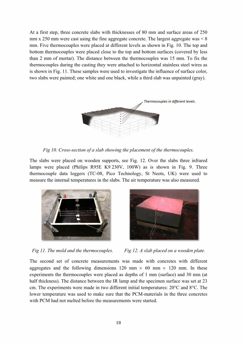
At a first step, three concrete slabs with thicknesses of 80 mm and surface areas of 250 mm x 250 mm were cast using the fine aggregate concrete. The largest aggregate was < 8 mm. Five thermocouples were placed at different levels as shown in Fig. 10. The top and bottom thermocouples were placed close to the top and bottom surfaces (covered by less than 2 mm of mortar). The distance between the thermocouples was 15 mm. To fix the thermocouples during the casting they were attached to horizontal stainless steel wires as is shown in Fig. 11. These samples were used to investigate the influence of surface color, two slabs were painted; one white and one black, while a third slab was unpainted (gray).

Fig 10. Cross-section of a slab showing the placement of the thermocouples.

The slabs were placed on wooden supports, see Fig. 12. Over the slabs three infrared lamps were placed (Philips R95E K9 230V, 100W) as is shown in Fig. 9. Three thermocouple data loggers (TC-08, Pico Technology, St Neots, UK) were used to measure the internal temperatures in the slabs. The air temperature was also measured.

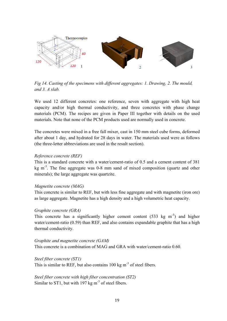
Fig 11. The mold and the thermocouples. Fig 12. A slab placed on a wooden plate.

The second set of concrete measurements was made with concretes with different

aggregates and the following dimensions 120 mm 60 mm 120 mm. In these experiments the thermocouples were placed as depths of 1 mm (surface) and 30 mm (at half thickness). The distance between the IR lamp and the specimen surface was set at 23 cm. The experiments were made in two different initial temperatures: 20°C and 8°C. The lower temperature was used to make sure that the PCM-materials in the three concretes with PCM had not melted before the measurements were started.

19

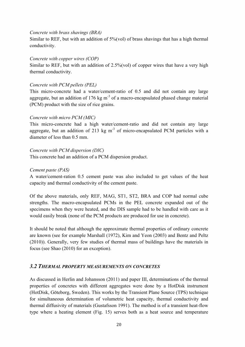
Fig 14. Casting of the specimens with different aggregates: 1. Drawing, 2. The mould, and 3. A slab. We used 12 different concretes: one reference, seven with aggregate with high heat capacity and/or high thermal conductivity, and three concretes with phase change materials (PCM). The recipes are given in Paper III together with details on the used materials. Note that none of the PCM products used are normally used in concrete. The concretes were mixed in a free fall mixer, cast in 150 mm steel cube forms, deformed after about 1 day, and hydrated for 28 days in water. The materials used were as follows (the three-letter abbreviations are used in the result section). Reference concrete (REF) This is a standard concrete with a water/cement-ratio of 0.5 and a cement content of 381 kg m-3. The fine aggregate was 0-8 mm sand of mixed composition (quartz and other minerals); the large aggregate was quartzite.

Magnetite concrete (MAG) This concrete is similar to REF, but with less fine aggregate and with magnetite (iron ore) as large aggregate. Magnetite has a high density and a high volumetric heat capacity. Graphite concrete (GRA) This concrete has a significantly higher cement content (533 kg m-3) and higher water/cement-ratio (0.59) than REF, and also contains expandable graphite that has a high thermal conductivity. Graphite and magnetite concrete (GAM) This concrete is a combination of MAG and GRA with water/cement-ratio 0.60. Steel fiber concrete (ST1) This is similar to REF, but also contains 100 kg m-3 of steel fibers. Steel fiber concrete with high fiber concentration (ST2) Similar to ST1, but with 197 kg m-3 of steel fibers.

20

Concrete with brass shavings (BRA) Similar to REF, but with an addition of 5%(vol) of brass shavings that has a high thermal conductivity. Concrete with copper wires (COP) Similar to REF, but with an addition of 2.5%(vol) of copper wires that have a very high thermal conductivity. Concrete with PCM pellets (PEL) This micro-concrete had a water/cement-ratio of 0.5 and did not contain any large aggregate, but an addition of 176 kg m-3 of a macro-encapsulated phased change material (PCM) product with the size of rice grains. Concrete with micro PCM (MIC) This micro-concrete had a high water/cement-ratio and did not contain any large aggregate, but an addition of 213 kg m-3 of micro-encapsulated PCM particles with a diameter of less than 0.5 mm. Concrete with PCM dispersion (DIC) This concrete had an addition of a PCM dispersion product. Cement paste (PAS) A water/cement-ration 0.5 cement paste was also included to get values of the heat capacity and thermal conductivity of the cement paste. Of the above materials, only REF, MAG, ST1, ST2, BRA and COP had normal cube strengths. The macro-encapsulated PCMs in the PEL concrete expanded out of the specimens when they were heated, and the DIS sample had to be handled with care as it would easily break (none of the PCM products are produced for use in concrete). It should be noted that although the approximate thermal properties of ordinary concrete are known (see for example Marshall (1972), Kim and Yeon (2003) and Bentz and Peltz (2010)). Generally, very few studies of thermal mass of buildings have the materials in focus (see Shao (2010) for an exception).

3.2 THERMAL PROPERTY MEASUREMENTS ON CONCRETES

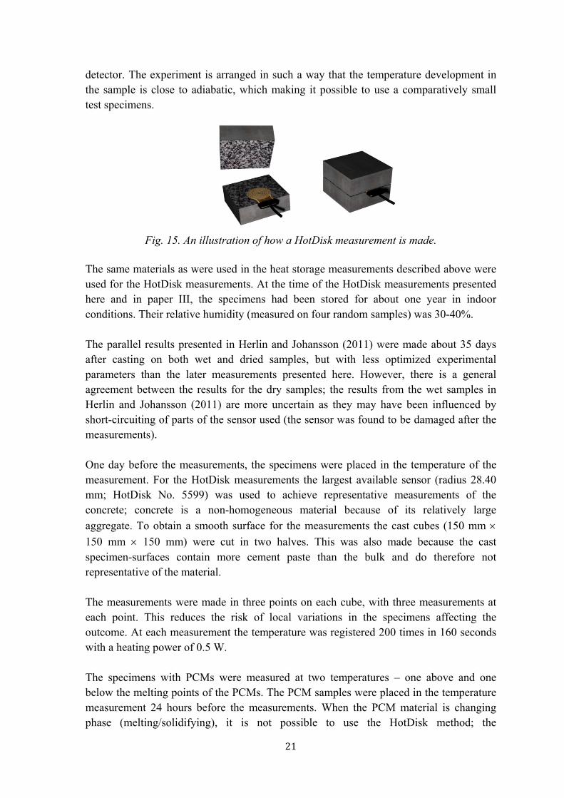
As discussed in Herlin and Johansson (2011) and paper III, determinations of the thermal properties of concretes with different aggregates were done by a HotDisk instrument (HotDisk, Göteborg, Sweden). This works by the Transient Plane Source (TPS) technique for simultaneous determination of volumetric heat capacity, thermal conductivity and thermal diffusivity of materials (Gustafsson 1991). The method is of a transient heat-flow type where a heating element (Fig. 15) serves both as a heat source and temperature

21

detector. The experiment is arranged in such a way that the temperature development in the sample is close to adiabatic, which making it possible to use a comparatively small test specimens.

Fig. 15. An illustration of how a HotDisk measurement is made.

The same materials as were used in the heat storage measurements described above were used for the HotDisk measurements. At the time of the HotDisk measurements presented here and in paper III, the specimens had been stored for about one year in indoor conditions. Their relative humidity (measured on four random samples) was 30-40%. The parallel results presented in Herlin and Johansson (2011) were made about 35 days after casting on both wet and dried samples, but with less optimized experimental parameters than the later measurements presented here. However, there is a general agreement between the results for the dry samples; the results from the wet samples in Herlin and Johansson (2011) are more uncertain as they may have been influenced by short-circuiting of parts of the sensor used (the sensor was found to be damaged after the measurements). One day before the measurements, the specimens were placed in the temperature of the measurement. For the HotDisk measurements the largest available sensor (radius 28.40 mm; HotDisk No. 5599) was used to achieve representative measurements of the concrete; concrete is a non-homogeneous material because of its relatively large

aggregate. To obtain a smooth surface for the measurements the cast cubes (150 mm

150 mm 150 mm) were cut in two halves. This was also made because the cast specimen-surfaces contain more cement paste than the bulk and do therefore not representative of the material. The measurements were made in three points on each cube, with three measurements at each point. This reduces the risk of local variations in the specimens affecting the outcome. At each measurement the temperature was registered 200 times in 160 seconds with a heating power of 0.5 W. The specimens with PCMs were measured at two temperatures – one above and one below the melting points of the PCMs. The PCM samples were placed in the temperature measurement 24 hours before the measurements. When the PCM material is changing phase (melting/solidifying), it is not possible to use the HotDisk method; the

22

measurements were therefore only made when the PCMs were either fully solid of fully liquid.

3.3 SIMULATION MODEL FOR THE INFLUENCE OF THERMAL INERTIA

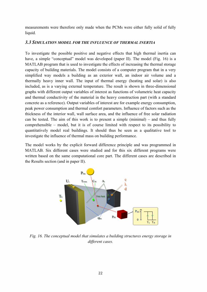
To investigate the possible positive and negative effects that high thermal inertia can have, a simple “conceptual” model was developed (paper II). The model (Fig. 16) is a MATLAB program that is used to investigate the effects of increasing the thermal storage capacity of building materials. The model consists of a computer program that in a very simplified way models a building as an exterior wall, an indoor air volume and a thermally heavy inner wall. The input of thermal energy (heating and solar) is also included, as is a varying external temperature. The result is shown in three-dimensional graphs with different output variables of interest as functions of volumetric heat capacity and thermal conductivity of the material in the heavy construction part (with a standard concrete as a reference). Output variables of interest are for example energy consumption, peak power consumption and thermal comfort parameters. Influence of factors such as the thickness of the interior wall, wall surface area, and the influence of free solar radiation can be tested. The aim of this work is to present a simple (minimal) – and thus fully comprehensible – model, but it is of course limited with respect to its possibility to quantitatively model real buildings. It should thus be seen as a qualitative tool to investigate the influence of thermal mass on building performance.

The model works by the explicit forward difference principle and was programmed in MATLAB. Six different cases were studied and for this six different programs were written based on the same computational core part. The different cases are described in the Results section (and in paper II).

Fig. 16. The conceptual model that simulates a building structures energy storage in different cases.

23

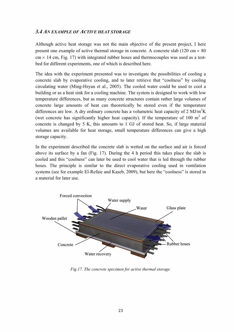
3.4 AN EXAMPLE OF ACTIVE HEAT STORAGE

Although active heat storage was not the main objective of the present project, I here

present one example of active thermal storage in concrete. A concrete slab (120 cm 80

cm 14 cm, Fig. 17) with integrated rubber hoses and thermocouples was used as a test-bed for different experiments, one of which is described here.

The idea with the experiment presented was to investigate the possibilities of cooling a concrete slab by evaporative cooling, and to later retrieve that “coolness” by cooling circulating water (Ming-Hsyan et al., 2005). The cooled water could be used to cool a building or as a heat sink for a cooling machine. The system is designed to work with low temperature differences, but as many concrete structures contain rather large volumes of concrete large amounts of heat can theoretically be stored even if the temperature differences are low. A dry ordinary concrete has a volumetric heat capacity of 2 MJ/m3K (wet concrete has significantly higher heat capacity). If the temperature of 100 m3 of concrete is changed by 5 K, this amounts to 1 GJ of stored heat. So, if large material volumes are available for heat storage, small temperature differences can give a high storage capacity.

In the experiment described the concrete slab is wetted on the surface and air is forced above its surface by a fan (Fig. 17). During the 4 h period this takes place the slab is cooled and this “coolness” can later be used to cool water that is led through the rubber hoses. The principle is similar to the direct evaporative cooling used in ventilation systems (see for example El-Refaie and Kaseb, 2009), but here the “coolness” is stored in a material for later use.

Fig.17. The concrete specimen for active thermal storage.

24

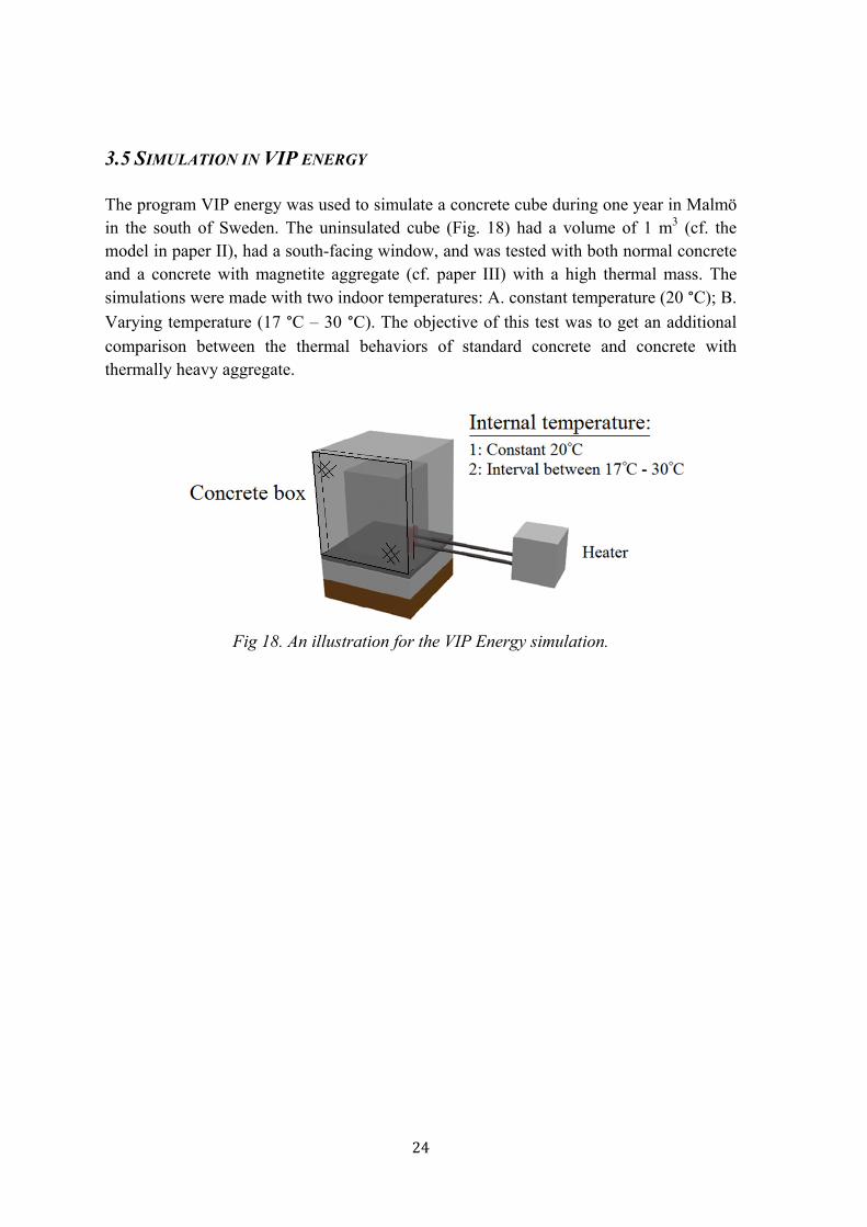
3.5 SIMULATION IN VIP ENERGY

The program VIP energy was used to simulate a concrete cube during one year in Malmö in the south of Sweden. The uninsulated cube (Fig. 18) had a volume of 1 m3 (cf. the model in paper II), had a south-facing window, and was tested with both normal concrete and a concrete with magnetite aggregate (cf. paper III) with a high thermal mass. The simulations were made with two indoor temperatures: A. constant temperature (20 °C); B.

Varying temperature (17 °C – 30 °C). The objective of this test was to get an additional

comparison between the thermal behaviors of standard concrete and concrete with thermally heavy aggregate.

Fig 18. An illustration for the VIP Energy simulation.

25

4 RESULTS 4.1 HEAT STORAGE MEASUREMENTS

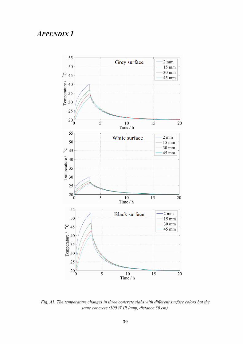
The results of the pre-study with IR radiation on concretes with different surface colors are presented in Appendix 1. The result was as expected and the highest temperature difference between black and white surfaces was 22 K.

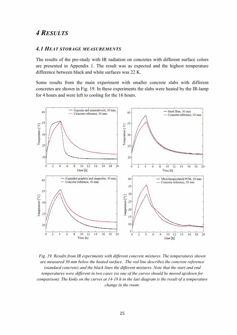
Some results from the main experiment with smaller concrete slabs with different concretes are shown in Fig. 19. In these experiments the slabs were heated by the IR-lamp for 4 hours and were left to cooling for the 16 hours.

Fig. 19. Results from IR experiments with different concrete mixtures. The temperatures shown are measured 30 mm below the heated surface. The red line describes the concrete reference

(standard concrete) and the black lines the different mixtures. Note that the start and end temperatures were different in two cases (so one of the curves should be moved up/down for

comparison). The kinks on the curves at 14-18 h in the last diagram is the result of a temperature change in the room.

26

The results (from left to right and from top to bottom) showed that:

- There was a significant delay in the temperature increase in a thermally heavy material, compared to in a light structure of insulation material (in this case mineral wool with a gypsum board).

- Steel fibers increase the thermal conductivity more than they increase the volumetric heat capacity, so the temperature response is slightly quicker for this concrete than for the reference concrete.

- The combination of magnetite and graphite increases the thermal conductivity slightly more than the volumetric heat capacity, giving a slightly quicker temperature response than the reference concrete.

- The addition of a phase change material (PCM) gives a distinctly different shape to the temperature curves; this is most easily seen during the cooling phase which the solidification significantly retards.

4.2 THERMAL PROPERTY MEASUREMENTS ON CONCRETES

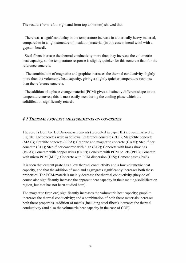
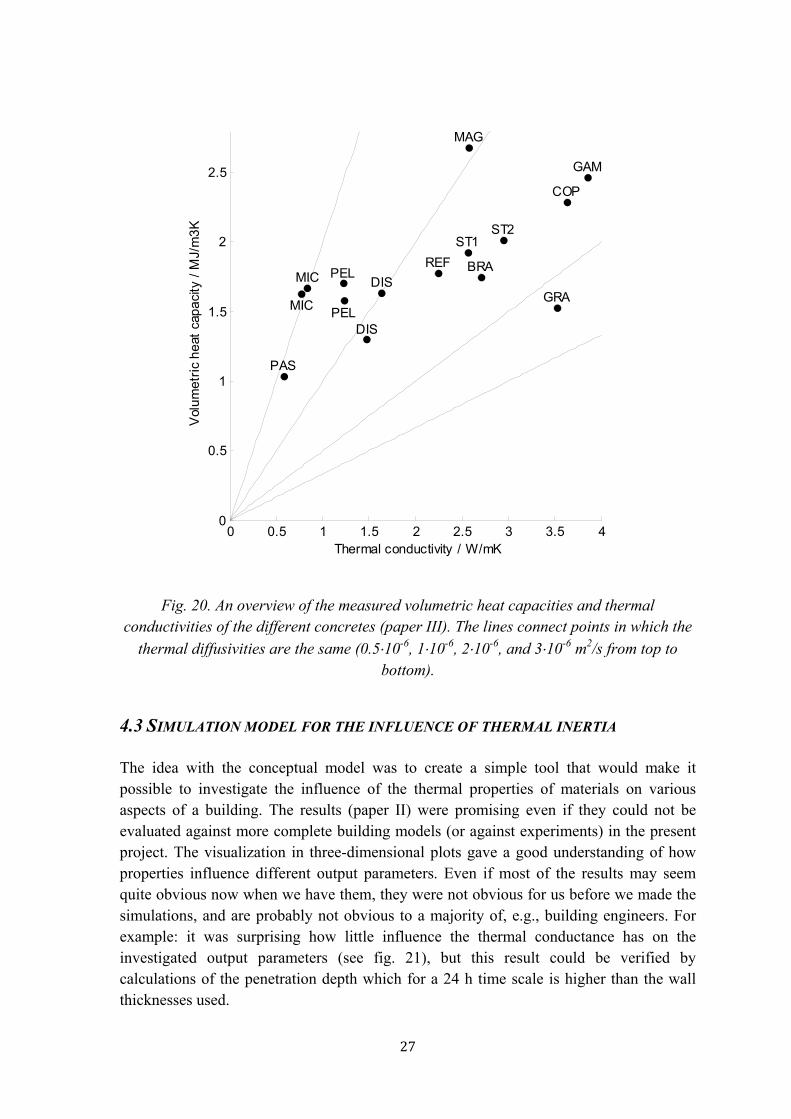
The results from the HotDisk-measurements (presented in paper III) are summarized in Fig. 20. The concretes were as follows: Reference concrete (REF); Magnetite concrete (MAG); Graphite concrete (GRA); Graphite and magnetite concrete (GAM); Steel fiber concrete (ST1); Steel fiber concrete with high (ST2); Concrete with brass shavings (BRA); Concrete with copper wires (COP); Concrete with PCM pellets (PEL); Concrete with micro PCM (MIC); Concrete with PCM dispersion (DIS); Cement paste (PAS).

It is seen that cement paste has a low thermal conductivity and a low volumetric heat capacity, and that the addition of sand and aggregates significantly increases both these properties. The PCM-materials mainly decrease the thermal conductivity (they do of course also significantly increase the apparent heat capacity in their melting/solidification region, but that has not been studied here).

The magnetite (iron ore) significantly increases the volumetric heat capacity; graphite increases the thermal conductivity; and a combination of both these materials increases both these properties. Addition of metals (including steel fibers) increases the thermal conductivity (and also the volumetric heat capacity in the case of COP).

27

Fig. 20. An overview of the measured volumetric heat capacities and thermal conductivities of the different concretes (paper III). The lines connect points in which the

thermal diffusivities are the same (0.510-6, 110-6, 210-6, and 310-6 m2/s from top to bottom).

4.3 SIMULATION MODEL FOR THE INFLUENCE OF THERMAL INERTIA

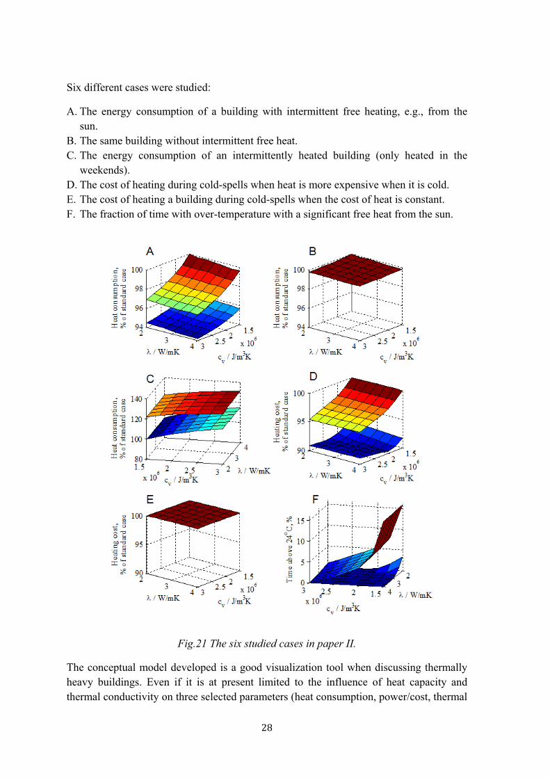
The idea with the conceptual model was to create a simple tool that would make it possible to investigate the influence of the thermal properties of materials on various aspects of a building. The results (paper II) were promising even if they could not be evaluated against more complete building models (or against experiments) in the present project. The visualization in three-dimensional plots gave a good understanding of how properties influence different output parameters. Even if most of the results may seem quite obvious now when we have them, they were not obvious for us before we made the simulations, and are probably not obvious to a majority of, e.g., building engineers. For example: it was surprising how little influence the thermal conductance has on the investigated output parameters (see fig. 21), but this result could be verified by calculations of the penetration depth which for a 24 h time scale is higher than the wall thicknesses used.

0 0.5 1 1.5 2 2.5 3 3.5 40

0.5

1

1.5

2

2.5

REF

MAG

GRA

ST1ST2

BRA

COP

GAM

PELDIS

MIC PELDIS

MIC

PAS

Thermal conductivity / W/mK

Vol

um

etr

ic h

eat

cap

aci

ty /

MJ/

m3

K

28

Six different cases were studied:

A. The energy consumption of a building with intermittent free heating, e.g., from the sun.

B. The same building without intermittent free heat. C. The energy consumption of an intermittently heated building (only heated in the

weekends). D. The cost of heating during cold-spells when heat is more expensive when it is cold. E. The cost of heating a building during cold-spells when the cost of heat is constant. F. The fraction of time with over-temperature with a significant free heat from the sun.

Fig.21 The six studied cases in paper II.

The conceptual model developed is a good visualization tool when discussing thermally heavy buildings. Even if it is at present limited to the influence of heat capacity and thermal conductivity on three selected parameters (heat consumption, power/cost, thermal

29

comfort) it can be tailored to different problems. However, the idea with the model is to keep it simple. If too many aspects of a building are added to make it more realistic, the increased complexity may limit its usefulness and one should then instead use models such as VIP+ or IDA that are more or less complete energy-models of a building. Some possible future versions of the conceptual model are:

A model with focus on the heating system, including the ventilation system with heat recovery.

A model with two zones, one south-facing and one north-facing, to investigate problems with over-heating of south-facing rooms.

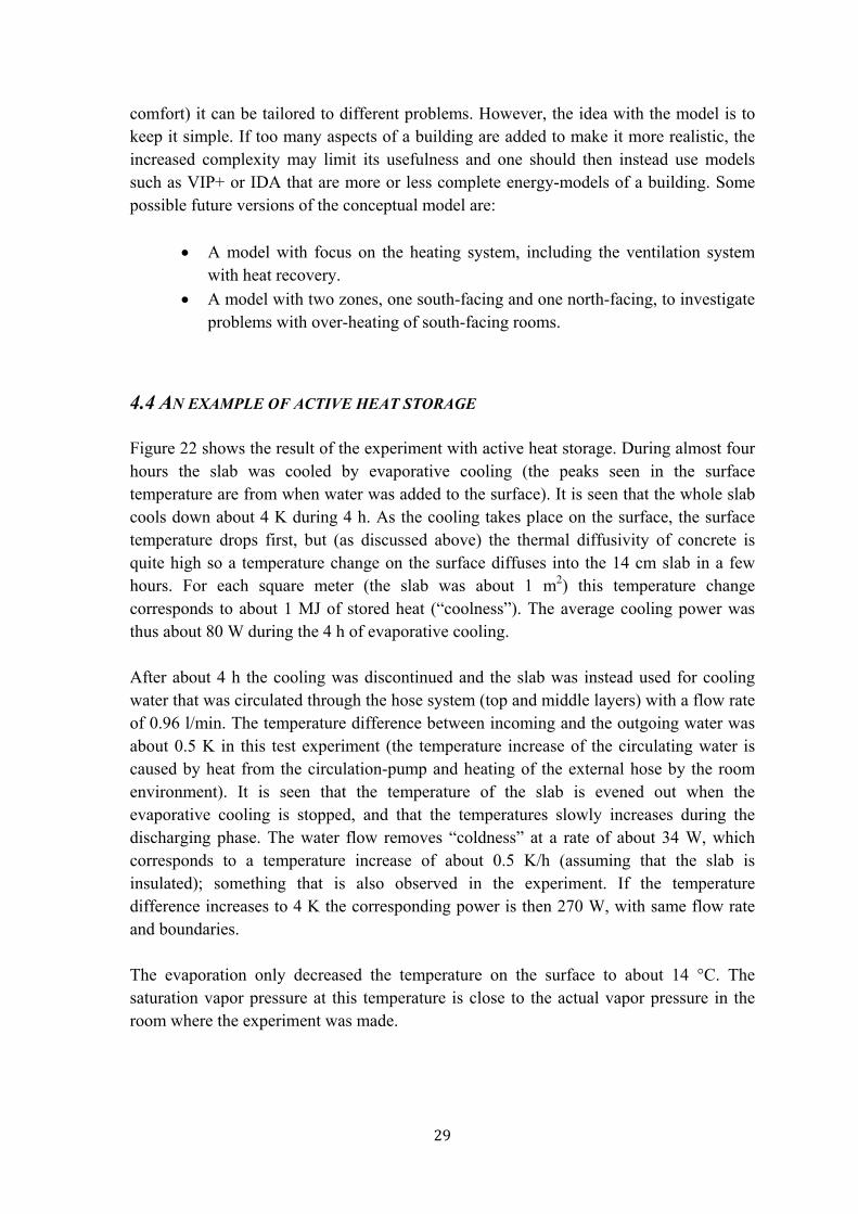
4.4 AN EXAMPLE OF ACTIVE HEAT STORAGE

Figure 22 shows the result of the experiment with active heat storage. During almost four hours the slab was cooled by evaporative cooling (the peaks seen in the surface temperature are from when water was added to the surface). It is seen that the whole slab cools down about 4 K during 4 h. As the cooling takes place on the surface, the surface temperature drops first, but (as discussed above) the thermal diffusivity of concrete is quite high so a temperature change on the surface diffuses into the 14 cm slab in a few hours. For each square meter (the slab was about 1 m2) this temperature change corresponds to about 1 MJ of stored heat (“coolness”). The average cooling power was thus about 80 W during the 4 h of evaporative cooling. After about 4 h the cooling was discontinued and the slab was instead used for cooling water that was circulated through the hose system (top and middle layers) with a flow rate of 0.96 l/min. The temperature difference between incoming and the outgoing water was about 0.5 K in this test experiment (the temperature increase of the circulating water is caused by heat from the circulation-pump and heating of the external hose by the room environment). It is seen that the temperature of the slab is evened out when the evaporative cooling is stopped, and that the temperatures slowly increases during the discharging phase. The water flow removes “coldness” at a rate of about 34 W, which corresponds to a temperature increase of about 0.5 K/h (assuming that the slab is insulated); something that is also observed in the experiment. If the temperature difference increases to 4 K the corresponding power is then 270 W, with same flow rate and boundaries. The evaporation only decreased the temperature on the surface to about 14 °C. The saturation vapor pressure at this temperature is close to the actual vapor pressure in the room where the experiment was made.

30

Fig. 22. The temperature on different levels in the concrete slab (a profile of the slab is shown on the right). The temperatures Tin and Tout represents the in- and outlet temperatures from the hoses. See the text for further explanations.

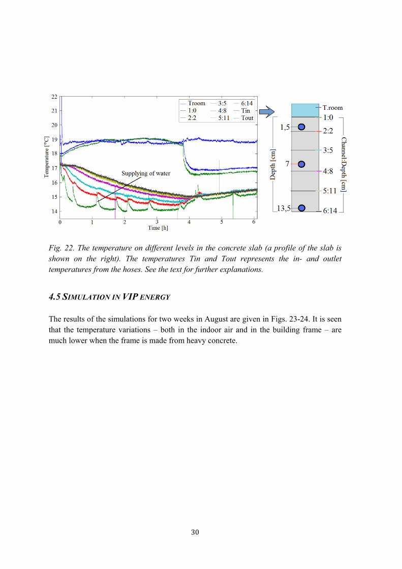
4.5 SIMULATION IN VIP ENERGY The results of the simulations for two weeks in August are given in Figs. 23-24. It is seen that the temperature variations – both in the indoor air and in the building frame – are much lower when the frame is made from heavy concrete.

31

Fig. 23. The temperature variation (indoor temperature: 17˚C-30˚C) when the cube consists of standard concrete.

Fig. 24. The temperature variation (indoor temperature: 17˚C-30˚C) when the cube consists of thermally heavy concrete.

32

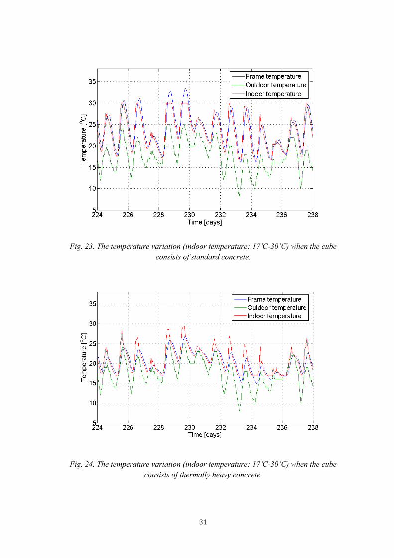
Fig. 25. The temperature variation (indoor temperature: 20˚C) when the cube consists of standard concrete.

Fig. 26. Tthe temperature variation (indoor temperature: 20˚C) when the cube consists of thermally heavy concrete.

33

5 DISCUSSION The total energy consumption of buildings in developed countries is estimated to be 20-40% of the total energy use (Pérez-Lombard and Pout, 2007). There is a large need to improve the energy performance of our buildings to fulfill the aim of reducing the global energy consumption and thus the related environmental impact. In cold climates the main way to decrease energy consumption is by improved insulation and airtightness of the building envelope and using heat recovery on the ventilation. It has been suggested that a further step towards low energy buildings is to increase the thermal mass inside the building envelope, an aspect that has been investigated in the present work. The thermal storage potential in a building material can influence a building’s energy consumption, power demand and thermal comfort. These aspects are coupled and at least if thermal comfort is interpreted as constant temperature, there is a conflict between thermal comfort and energy and power savings, as the latter demands temperature variations. The most discussed issue concerning heavy buildings is probably that they can reduce the energy consumption (we here only discuss passive storage in the building, i.e., without active thermal storage or other technically more advances solutions). One of our simulations (A) in paper II indicated that savings are possible under certain conditions (the 5% saving calculated should not be taken as a quantitative fact as the simulation model is simple). The studied case with free solar heating is an example of such a condition, but for this to take place the building has to be suitably arranged to accumulate the short term free heat; for example by large windows facing uncovered black concrete floors and walls. It must also be remembered that the internal temperature of a building needs to fluctuate in order for heat storage to take place; the heating system must therefore allow this to take place. We therefore need intelligent control systems that can take advantage of thermally heavy structures. A possibly more important aspect of high thermal mass and energy savings is to lower the peak power demands. A building with a high time constant does not need as high powers and such a continuous heat supply, as does a light building. This also enables the use of environmentally friendly low exergy energy sources with a small temperature difference between the heating or cooling media and the indoor air. As higher thermal mass buildings have higher time constants – that is, they change their temperature slowly – they do not need continuous heating (or cooling), but heating can instead to some extent take place when energy is available or when its cost is low. The most typical example in a cold climate is probably a cold spell during which buildings with low time constants need to be supplied with heat so that their internal temperatures will not decrease. A high time constant building – in which one also can allow a certain temperature decrease to take place – can get on without heat input during at least short cold spells. This is a significant advantage as peak energy production – which is most expensive and least environmentally friendly – can be reduced. However, to give thermally heavy buildings this legitimate advantage, the short-term price the user (=the building) pays must reflect

34

the price that the energy distributor has to pay. This is not the case today, but will probably be in the future. Thermally heavy buildings can also be designed with smaller heat distribution systems as they do not need to quickly respond to changes in the external temperature or internal loads. This can lead to decreased building costs. Possibly the same is true for heat distribution systems – like district heating pipes – if a district has a high proportion of thermally heavy buildings. These do not have to be dimensioned to supply the instantaneous heat consumption during a cold spell as a large part of the used heat is already in the buildings in the form of stored heat in the building structure. From the energy distributors point of view a thermally heavy building stock can be seen as a heat storage from which they (or rather the owners of the buildings) can retrieve heat if they do not have enough power capacity during a certain period like a cold spell or when energy consumption is high for other reasons, like in week-day mornings when many people shower at the same time. The third aspect of thermally heavy buildings is the increased thermal comfort, but as mentioned above, this requires heating control system that allows some degrees of temperature fluctuations to take place. Nevertheless is thermal comfort an important aspect of thermally heavy buildings as they can reduce over-heating by taking up excess free heat from for example solar radiation or office machines. This can be of particular importance in low-energy houses (zero-energy houses, passive buildings) as such buildings frequently experience over-temperatures. The most common thermally heavy building material is concrete. We have therefore performed this work with a focus on the thermal properties of concrete and whether these can be improved towards higher thermal conductivity and higher heat capacity (paper III). It was shown that both heat capacity and thermal conductivity can be increased by at least 50% by including high heat capacity materials (for example magnetite, iron ore) and high thermal conductance materials (for example graphite). No economical analysis of the use of such concretes has been made in the present project, but it is probable that such concrete will be significantly more expensive than standard concrete, and that this will limit their use. Note also that standard concrete does have a high volumetric heat capacity compared to other construction materials and is therefore useful in buildings to give high thermal inertia; so these materials with improved thermal properties may only be of interest in special applications. The main findings of this study were:

A combination of thermally heavy structures, variable energy prices, and intelligent control systems can provide significant economic and environmental benefits.

35

A conceptual model was developed to investigate the influence of the thermal properties of materials on various aspects of a building.

It is possible to significantly improve the thermal properties of concrete.

36

37

6 REFERENCES

Al-Sanea, S. A., M. F. Zedan, et al. (2012). "Effect of thermal mass on performance of insulated building walls and the concept of energy savings potential." Appl. Energy 89: 430-442.

Al-Temeemi, A. A. and D. J. Harris (2004). "A guideline for assessing the suitability of earth-sheltered mass-housing in hot-arid climates." Energy Build. 36(3): 251-260.

Antonopoulous, K. A. and C. Tzivanidis (1996). "Finite-difference prediction of transient indoor temperature and related correlation based on the building time constant." Int. J. Energy Res. 20: 507-520.

Balaras, C. A. (1996). "The role of thermal mass on the coolling load of buildings. An overview of computational methods." Energy Build. 24: 1-10.

Bellamy, L. A. and D. W. Mackenzie (2001). Thermal performance of buildings with heavy walls, BRANZ, New Zealand.

Bentz, D., M. A. Peltz, et al. (2011). "Thermal properties of high-volume fly ash mortars and concretes." J. Build. Phys. 34(3): 263-275.

Bloomfield, D. P. and D. J. Fisk (1977). "The optimisation of intermittent heating." Build. Environ. 12: 43-55.

Claesson J, 2003. Dynamic thermal networks: a methodology to account for time-dependent heat conduction. Proceedings of the 2nd International Conference on Research in Building Physics, Leuven, Belgium, p. 407-415. ISBN 90 5809 565 7

El-Refaie, M. F. and Kaseb, S. (2009) ”Speculation in the feasibility of evaporative cooling” Building and Environment 44 (2009) 826–838

Fernández, J. L., M. A. Porta-Gándara, et al. (2005). "Rapid on-site evaluation of thermal comfort through heat capacity in buildings." Energy Build. 37: 1205-1211.

Gustafsson, S (1991) ”Transient plane source techniques for thermal conductivity and thermal diffusivity measurements of solid materials”, Rev. Sci. Instrum. 62 (3), March 1991, 797-804.

Herlin, A., and Johansson, G. (2011) “A study of the possibilities to increase the heat storage capacity of concrete” (in Swedish), Master project report TVBM-5080, Building Materials, Lund University, Sweden

Kim, K.-H., S.-E. Jeon, et al. (2003). "An experimental study of thermal conductivity of concrete." Cement Concrete Res. 33: 363-371.

Li, Y. and P. Xu (2006). "Thermal mass design in buildings - heavy or light?" Int. J. Ventilation 5(1): 143-149.

Marshall, A. (1972). "The thermal properties of concrete." Build. Sci. 7: 167-174.

38

Ming-Hsyan, S., H. Ming-Jer, and C. Cha'o-Kuang (2005) ”A study of the liquid evaporation with Darcian resistance effect on mixed convection in porous media”. Int. Comm. Heat Mass Transfer,. 32(5) 685-694.

Luis Pérez-Lombard, J. O., C. Pout (2007). "A review on buildings energy consumption information." Energy and Buildings 40 (2008): 394-398.

Pupeikis, D., A. Burlingis, et al. (2010). "Required additional heating power of building during intermitted heating." J. Civ. Eng. Management 16(1): 141-148.

Sahar N. Kharrufa, Y. A. (2011). "Upgrading the building envelope to reduce cooling loads", The International Conference on Sustainable Systems and the Environment, American University of Sharjah, United Arab Emirates.

Shao, L. (2010). Materials for energy efficiency and thermal comfort in new buildings, . Materials for energy efficency and thermal comfort in buildings. M. R. Hall. Oxford, UK, Woodhead Publ. Ltd.: 631-648.

Yam, J., Y. Li, et al. (2003). "Nonlinear coupling between thermal mass and natural ventilation in buildings." Int. J. Heat Mass Transf. 47: 1251-1264.

Yang, L. and Y. Li (2008). "Cooling load reduction by using thermal mass and night ventilation." Energy Build. 40: 2052-2058.

Zhou, J., G. Zhang, et al. (2008). "Coupling of thermal mass and natural ventilation in buildings." Energy Build. 40: 979-986.

39

APPENDIX 1

Fig. A1. The temperature changes in three concrete slabs with different surface colors but the same concrete (100 W IR lamp, distance 30 cm).

40

PAPER I E.-L. W. Kurkinen and J. Karlsson “Different materials with high thermal mass and its influence on a building’s heat loss – an analysis based on the theory of dynamic thermal networks”, Proceedings of the 5th International Building Physics Conference (IBPC), 28-31 May 2012, Kyoto University, Japan (accepted).

I

Different Materials with High Thermal Mass and its Influence on a Building’s Heat Loss – An Analysis based on the Theory of Dynamic

Thermal Networks

Eva-Lotta W Kurkinen 1, Jonathan Karlsson 2

1Section of Building Physics and Indoor Environment, SP Technical Research Institute of Sweden 2 Division of Building Materials. Lund University, Box 118, 221 00 Lund, Sweden

Keywords: Thermal mass, heat loss, materials, response functions, Dynamic thermal networks

ABSTRACT

The time-dependent heat loss through a building exposed to variable outdoor and indoor temperatures depends on the properties of the buildings envelope and its material. It may be beneficial to use high thermal mass in a buildings frame construction with respect to energy consumption and thermal comfort. The thermal memory effect of light and heavy constructions are well known, but is this effect significant for a buildings energy consumption and indoor temperature? In this paper we study the effect of different high thermal mass materials on the annual heat loss and indoor temperature for a building located in Gothenburg, Sweden. The high thermal mass materials are concretes with different aggregates such as magnetite, expanded graphite, steel fiber and copper fiber.

The analysis was performed with the Dynamic Thermal Networks theory, which is based on step-response and weighting functions. The significance of the shape of the response and weighting functions on a buildings annual heat loss is studied in order to find the material or material combination that results in the shape of the most optimal response function.

The analysis shows that there is a different thermal behaviour between the different high thermal mass materials, but the differences are too small to have an effect on the studied buildings annual heat loss and indoor temperature.

1. Introduction

The time-dependent heat loss through a building exposed to variable outdoor and indoor temperatures depends on the properties of the walls, materials and their layers. The thermal memory effect of light and heavy walls, effects of temperature variation on different time scales, etc, represent a basic problem in building physics. Several studies have been made to investigate the significance of the order of wall layers on the buildings thermal behaviour and heat loss: Kossecka, Kosny (1998), Ghrab-Marcos (1991) and Boji´c, Loveday (1997).

In this paper the theory of Dynamic Thermal Network is used to calculate the heat consumption rate needed-, to keep the indoor temperature around 20 oC, for a building with different thermal mass in the construction. The building's response and weighting functions are needed for the calculations (Claesson 2003). These functions give information about the buildings thermal behaviour. By changing the aggregate in the concrete used in an external wall-, the weighting function will change while the buildings U-value is still the same. In a numerical solution, we must use a discrete approximation. The buildings weighting functions are divided into weighting factors. A weighting factor is the average value of the weighting function during a time step h.

In this paper the shape of the weighting functions and the values of the weighting factors are compared with the buildings annual heat loss and indoor temperature variation. The significance of the shape of the response and weighting functions on the buildings annual heat loss is studied in order to find the material or material combination that results in the

most optimal shape of the response function. Which material and material properties gives the most suitable indoor temperature and lowest energy consumption?

2. Dynamic thermal network

The dynamic heat loss of a building is the sum of an absorptive and a transmittive heat flux. Figure 1 shows the dynamic thermal network for a building’s heat loss. The indoor temperature T1(t) is connected to the outdoor temperature T2(t) by the buildings thermal conductance K12, this is the transmittive part. There is also an absorptive part with a heat flux over the surface conductance K1. Summation signs are added to the conductance symbols. The signs signify that it is a dynamic case and that we have to take an average of the node temperatures according to (2).

12K 2 ( )T t1( )T t

1K

1( )Q t

Fig. 1. Dynamic thermal network for the buildings heat loss.

2.1 Basic formula

The dynamic heat loss of a building according to Figure 1 is:

1 1 1 1a 12 1t 2t( ) ( ) ( ) ( ) ( )Q t K T t T t K T t T t (1)

The (steady-state) thermal conductance for the whole building is K12 (W/K). The factor K1 is the surface heat transfer coefficient at the buildings inside. It is equal to the

surface area A1 times the surface heat transfer coefficient 1:

1 1 1K A . The temperatures that are used are the indoor

temperature T1(t) and average temperatures backward in time. The temperature averages are given by:

1a 1a 1

0

( ) ( ) ( )T t T t d

1t 12 1

0

( ) ( ) ( )T t T t d

(2)

2t 12 2

0

( ) ( ) ( )T t T t d

Here, assume values from zero to infinity or sufficiently far back in time to give stable solutions. The absorptive weighting function 1a ( ) and the transmittive weighting

function 12 ( ) are discussed below.

2.2 Step-response and weighting functions

The weighting functions for preceding boundary temperatures in (2) are obtained from a step-response solution (Claesson 2003). The temperature at the inside is changed from zero to one, while the outdoor surface is kept at zero. Let Q12() be the outward heat flux at the outside and Q11() the inward heat flux at the building’s inside. We use the time in order to distinguish it from the current time t in (2). The transmittive part, Q12(), is zero at the very beginning, and it increases to the steady-state value K12 after long time. The heat flux at the inside, Q11(), starts with the high value K1 and decreases to the same steady-state value K12. In the calculations we will use the transmittive response flux and the following absorptive response flux:

1a 11 12( ) ( ) ( )Q Q Q (3)

This response flux starts with a high value (K1) and decreases to zero.

The weighting functions are the derivative of the response heat fluxes divided with their respective thermal conductance.

1a1a

1

( )1( )

dQ

K d

, 12

1212

1( )

dQ

K d

(4)

The weighting functions are positive and their integrals become equal to one.

2.3 Discrete approximation

In a numerical solution, we must use a discrete approximation. Let h>0 be the time step. The time interval under consideration, nh h t nh , has index n. The preceding intervals, nh h h t nh h , are enumerated backwards in time ( = 1, 2, …). We consider a linear temperature variation during each time step with the temperature 1, 1( )nT T nh h at the right hand end point

of interval n-. The heat flux at the considered time is

1, 1( )nQ Q nh . In discrete form we have:

1, 1 1, 1a, 12 1t, 2t,n n n n nQ K T T K T T (5)

In the discrete form of (2), we get the following average values of the boundary temperatures:

1a, 1a, 1,1

s

n nT T

1t, 12, 1,0

s

n nT T

(6)

2t, 12, 2,0

s

n nT T

Relations (5) and (6) are the discrete form of (1) and (2) for the dynamic thermal network in Figure 1. The surface conductances are replaced by modified surface conductances and the weighting functions by weighting factors for each time step. The integration to infinity in the temperature averages (2) must be limited to a finite value s at which time the weighting functions are zero with a sufficient accuracy. Then steady-state conditions are attained within the considered accuracy. The summations are performed up to a large = s with s=s/h We use time-step averages 1a ( )Q

and 12 ( )Q of the response functions 1a ( )Q and 12 ( )Q :

1a 1a1

( ) ( ') 'h

Q Q dh

, 12 121

( ) ( ') 'h

Q Q dh

(7)

The modified surface conductance 1K is:

1 1a (0)K Q (8)

From (2) with piece-wise linear boundary temperatures, we get the weighting factors (Claesson 2003):

1a 1a1a,

1

( ) ( )Q h h Q h

K

12 1212,

12

( ) ( )Q h Q h h

K

(9)

3. Studied building

The studied building is a student building with two floors and four single rum apartments on each floor, see Figure 2a and 2b. The building is located in Gothenburg the south west part of Sweden. Only the second floor is considered in this study. Table 1 shows the data of the building. The building's total U-value for the studied part is 0.26 W/m2K.

Fig. 2a. Sectional drawing of the studied building.

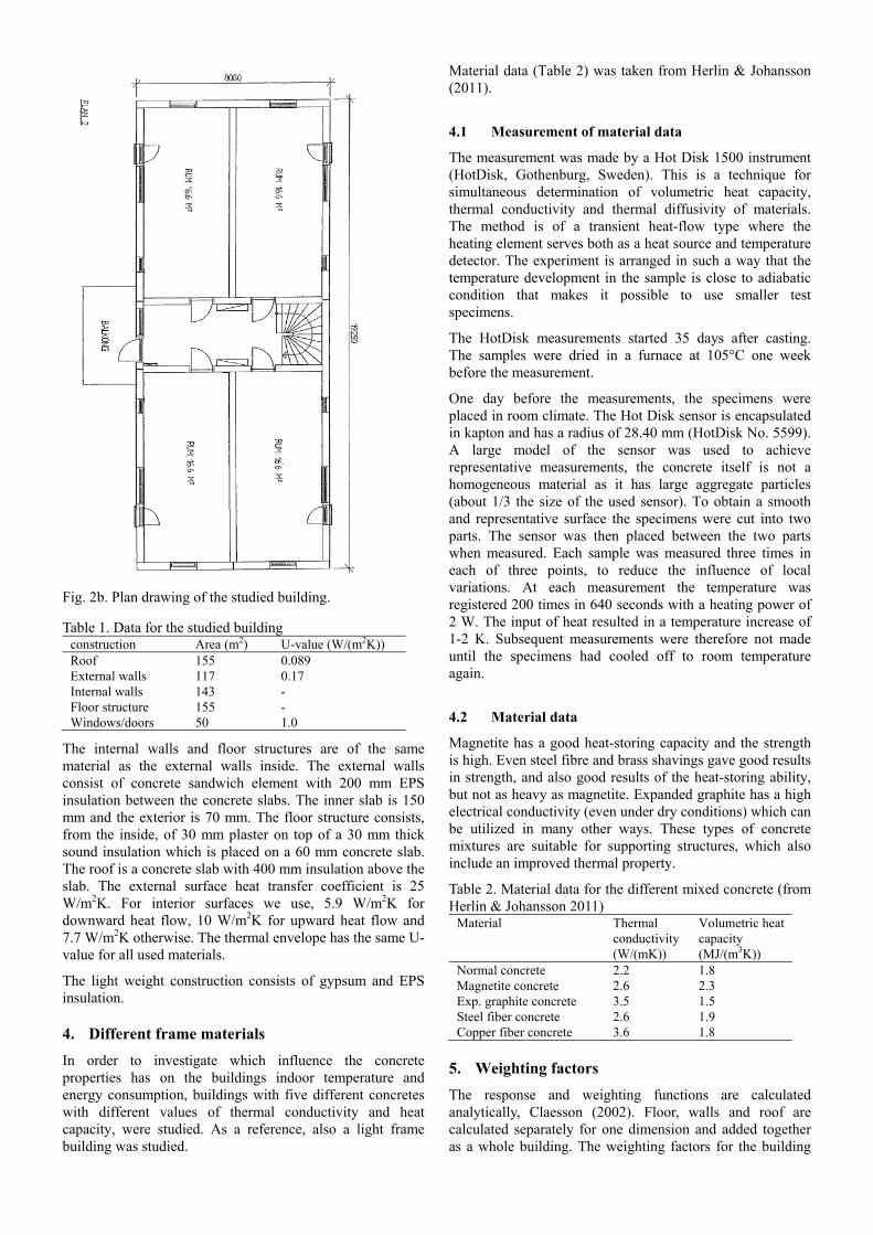
Fig. 2b. Plan drawing of the studied building.

Table 1. Data for the studied building construction Area (m2) U-value (W/(m2K)) Roof 155 0.089 External walls 117 0.17 Internal walls 143 - Floor structure 155 - Windows/doors 50 1.0

The internal walls and floor structures are of the same material as the external walls inside. The external walls consist of concrete sandwich element with 200 mm EPS insulation between the concrete slabs. The inner slab is 150 mm and the exterior is 70 mm. The floor structure consists, from the inside, of 30 mm plaster on top of a 30 mm thick sound insulation which is placed on a 60 mm concrete slab. The roof is a concrete slab with 400 mm insulation above the slab. The external surface heat transfer coefficient is 25 W/m2K. For interior surfaces we use, 5.9 W/m2K for downward heat flow, 10 W/m2K for upward heat flow and 7.7 W/m2K otherwise. The thermal envelope has the same U-value for all used materials.

The light weight construction consists of gypsum and EPS insulation.

4. Different frame materials

In order to investigate which influence the concrete properties has on the buildings indoor temperature and energy consumption, buildings with five different concretes with different values of thermal conductivity and heat capacity, were studied. As a reference, also a light frame building was studied.

Material data (Table 2) was taken from Herlin & Johansson (2011).

4.1 Measurement of material data

The measurement was made by a Hot Disk 1500 instrument (HotDisk, Gothenburg, Sweden). This is a technique for simultaneous determination of volumetric heat capacity, thermal conductivity and thermal diffusivity of materials. The method is of a transient heat-flow type where the heating element serves both as a heat source and temperature detector. The experiment is arranged in such a way that the temperature development in the sample is close to adiabatic condition that makes it possible to use smaller test specimens.

The HotDisk measurements started 35 days after casting. The samples were dried in a furnace at 105°C one week before the measurement.

One day before the measurements, the specimens were placed in room climate. The Hot Disk sensor is encapsulated in kapton and has a radius of 28.40 mm (HotDisk No. 5599). A large model of the sensor was used to achieve representative measurements, the concrete itself is not a homogeneous material as it has large aggregate particles (about 1/3 the size of the used sensor). To obtain a smooth and representative surface the specimens were cut into two parts. The sensor was then placed between the two parts when measured. Each sample was measured three times in each of three points, to reduce the influence of local variations. At each measurement the temperature was registered 200 times in 640 seconds with a heating power of 2 W. The input of heat resulted in a temperature increase of 1-2 K. Subsequent measurements were therefore not made until the specimens had cooled off to room temperature again.

4.2 Material data

Magnetite has a good heat-storing capacity and the strength is high. Even steel fibre and brass shavings gave good results in strength, and also good results of the heat-storing ability, but not as heavy as magnetite. Expanded graphite has a high electrical conductivity (even under dry conditions) which can be utilized in many other ways. These types of concrete mixtures are suitable for supporting structures, which also include an improved thermal property.

Table 2. Material data for the different mixed concrete (from Herlin & Johansson 2011)

Material Thermal conductivity (W/(mK))

Volumetric heat capacity (MJ/(m3K))

Normal concrete 2.2 1.8 Magnetite concrete 2.6 2.3 Exp. graphite concrete 3.5 1.5 Steel fiber concrete 2.6 1.9 Copper fiber concrete 3.6 1.8

5. Weighting factors

The response and weighting functions are calculated analytically, Claesson (2002). Floor, walls and roof are calculated separately for one dimension and added together as a whole building. The weighting factors for the building

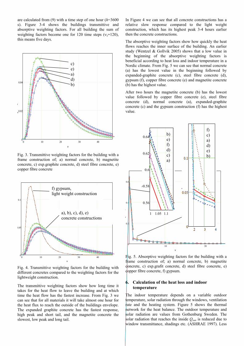
are calculated from (9) with a time step of one hour (h=3600 s). Figure 3-4 shows the buildings transmittive and absorptive weighting factors. For all building the sum of weighting factors become one for 120 time steps (s=120), this means five days.

0 10 20 30 400

0.02

0.04

ν

ν

ν

ν

Fig. 3. Transmittive weighting factors for the building with a frame construction of; a) normal concrete, b) magnetite concrete, c) exp.graphite concrete, d) steel fibre concrete, e) copper fibre concrete

0 10 20 30 400

0.05

0.1

ν Fig. 4. Transmittive weighting factors for the building with different concretes compared to the weighting factors for the lightweight construction.

The transmittive weighting factors show how long time it takes for the heat flow to leave the building and at which time the heat flow has the fastest increase. From Fig. 3 we can see that for all materials it will take almost one hour for the heat flux to reach the outside of the buildings envelope. The expanded graphite concrete has the fastest response, high peak and short tail, and the magnetite concrete the slowest, low peak and long tail.

In Figure 4 we can see that all concrete constructions has a relative slow response compared to the light weight construction, which has its highest peak 3-4 hours earlier then the concrete constructions.

The absorptive weighting factors show how quickly the heat flows reaches the inner surface of the building. An earlier study (Wentzel & Gollvik 2005) shows that a low value in the beginning of the absorptive weighting factors is beneficial according to heat loss and indoor temperature in a Nordic climate. From Fig. 5 we can see that normal concrete (a) has the lowest value in the beginning followed by expanded-graphite concrete (c), steel fibre concrete (d), gypsum (f), copper fibre concrete (e) and magnetite concrete (b) has the highest value.

After two hours the magnetite concrete (b) has the lowest value followed by copper fibre concrete (e), steel fibre concrete (d), normal concrete (a), expanded-graphite concrete (c) and the gypsum construction (f) has the highest value.

10 200

0.2

0.4

0.6

ν

ν

ν Fig. 5. Absorptive weighting factors for the building with a frame construction of; a) normal concrete, b) magnetite concrete, c) exp.grafit concrete, d) steel fibre concrete, e) copper fibre concrete, f) gypsum.

6. Calculation of the heat loss and indoor temperature

The indoor temperature depends on a variable outdoor temperature, solar radiation through the windows, ventilation rate and the heating system. Figure 5 shows the thermal network for the heat balance. The outdoor temperature and solar radiation are values from Gothenburg Sweden. The solar radiation that reaches the inside Qsun is reduced due to window transmittance, shadings etc. (ASHRAE 1997). Less

c) e) a) d) b)

1 1.05 1.1

0.56

0.58

0.6

0.62

0.64

ν

νf) gypsum, light weight construction

b) e) f) d) c) a)

f) c) a) d) e) b)

a), b), c), d), e) concrete constructions

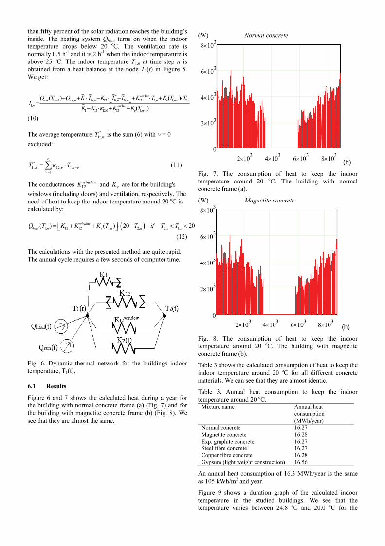
than fifty percent of the solar radiation reaches the building’s inside. The heating system Qheat turns on when the indoor temperature drops below 20 oC. The ventilation rate is normally 0.5 h-1 and it is 2 h-1 when the indoor temperature is above 25 oC. The indoor temperature T1,n at time step n is obtained from a heat balance at the node T1(t) in Figure 5. We get:

*

1, 1 , 1 1a, 12 1t, 2t, 12 2, 1, 1 2,

1,1 12 12,0 12 1, 1

( ) ( )

( )

windowheat n sun n n n n n v n n

n windowv n

Q T Q K T K T T K T K T TT

K K K K T

(10) The average temperature *

1t,nT is the sum (6) with = 0

excluded:

s*

1t, 12, 1,1

n nT T

(11)

The conductances 12windowK and vK are for the building's

windows (including doors) and ventilation, respectively. The need of heat to keep the indoor temperature around 20 oC is calculated by:

1, 12 12 1, 2, 2, 1,( ) ( ) 20 20windowheat n v n n n nQ T K K K T T if T T

(12) The calculations with the presented method are quite rapid. The annual cycle requires a few seconds of computer time.

Fig. 6. Dynamic thermal network for the buildings indoor temperature, T1(t).

6.1 Results

Figure 6 and 7 shows the calculated heat during a year for the building with normal concrete frame (a) (Fig. 7) and for the building with magnetite concrete frame (b) (Fig. 8). We see that they are almost the same.

(W) Normal concrete

2 103 4 10

3 6 103 8 10

30

2 103

4 103

6 103

8 103

(h)

Fig. 7. The consumption of heat to keep the indoor temperature around 20 oC. The building with normal concrete frame (a).

(W) Magnetite concrete

2 103 4 10

3 6 103 8 10

30

2 103

4 103

6 103

8 103

(h)

Fig. 8. The consumption of heat to keep the indoor temperature around 20 oC. The building with magnetite concrete frame (b).

Table 3 shows the calculated consumption of heat to keep the indoor temperature around 20 oC for all different concrete materials. We can see that they are almost identic.

Table 3. Annual heat consumption to keep the indoor temperature around 20 oC.

Mixture name Annual heat consumption (MWh/year)

Normal concrete 16.27 Magnetite concrete 16.28 Exp. graphite concrete 16.27 Steel fibre concrete 16.27 Copper fibre concrete 16.28 Gypsum (light weight construction) 16.56

An annual heat consumption of 16.3 MWh/year is the same as 105 kWh/m2 and year.

Figure 9 shows a duration graph of the calculated indoor temperature in the studied buildings. We see that the temperature varies between 24.8 oC and 20.0 oC for the

studied frame materials of concrete. The lines are almost perfectly superimposed and therefor impossible to separate. The thin black line shows the indoor temperature for the light weight construction. That temperature varies between 26.0 oC and 19.9 oC.

The temperature variation is more beneficial for the different concrete constructions then for the light weight construction.

(oC)

(h)

Fig. 9. The indoor temperature during a whole year for the studied building different concrete combinations in the frame.

7. The influence of thermal mass on the shape of the weighting factors and on the buildings heat loss

By studying the weighting factors for the different frame materials we can see that they have different thermal behaviour. For example, the transmittive heat flow through the expanded graphite concrete construction is more rapid than for the magnetit concrete construction. The absorptive weighting factors show that the magnetite concrete responds faster on a temperature change in the indoor temperature than what for example normal concrete does. The construction with magnetite concrete has the highest value for the first absorptive weighting factor. The construction with normal concrete has the lowest value for the first absorptive weighting factor, see Fig 5. Due Based on a previous investigation (Wentzel & Gollvik 2005) this should mean that the normal concrete is more beneficial than the magnetite concrete with respect to heat consumption and indoor temperature. Unfortunately the difference in this analysis is too small to have an influence on the buildings heat consumption. But we can still see a trend that a low first value on the absorptive weighting factor is beneficial on the heat consumption and indoor temperature.

8. Conclusions

The analysis shows that there is a different thermal behaviour between the different high thermal mass materials, but the differences are too small to have an effect on the studied buildings annual heat loss and indoor temperature.

The effect of thermal mass in the frame construction will probably have bigger influence on the heat loss and indoor

temperature, if the buildings heating system is optimised for it.

The knowledge of older buildings and structures tend to reflect our knowledge of system thinking and the use of thermal inertia. Building traditions in various climate conditions gives us new knowledge about adjustments to our system solutions, system solutions in the sense that the materials function in relation to indoor environment work together in an intelligent way.

Acknowledgements

This article is part of a large research consortia concerning frame material and energy consumption in Nordic climate (Saving energy by using the thermal properties of heavy-frame buildings based on new materials, constructions and heat storage systems). This research is mainly financed by CERBOF (Centre for energy and resource efficiency in the built environment) and Cementa AB in Sweden.

References

ASHRAE Handbook of Fundamentals. 1997. Am. Soc. Of Heationg, refrigeration, and Air Conditioning Engineers, Atlanta GA

Boji´c M.Lj, Loveday D.L, 1997. The Influence on Building Thermal Behavior of the Insulation/Masonry Distribution in a Three-Layered Construction. Energy and Buildings, 26, No. 2, p. 153-157

Claesson J, 2002. Heat Conduction in Composite Walls. Rapid Solutions Combining Fourier and Laplace Techniques. Proceedings of the 6th Symposium on Building Physics in the Nordic Countries Trondheim. Norway, p. 119-126. ISBN 82-91412-02-2

Claesson J, 2003. Dynamic thermal networks: a methodology to account for time-dependent heat conduction. Proceedings of the 2nd International Conference on Research in Building Physics, Leuven, Belgium, p. 407-415. ISBN 90 5809 565 7

Ghrab-Marcos N, 1991. Energy and Financial Considerations Related to Wall Design for a Conditioned Cell in Tunisian Conditions. Renewable Energy, 1, No. 1, p.145-159.

Herlin A, Johansson G, 2011. A Study of the Possibility to Increase the Heat-Storing Capacity of Concrete (in Swedish). Diploma work at Lunds Technical University, department of Building Materials, Sweden. ISRN: 0348-7911 TVBM

Kossecka E, Kosny J, 1998. Effect of Insulation and Mass Distribution in Exterior Walls on Dynamic Thermal Performance of Whole Buildings, Proceedings of the Buildings VII Conference, Clear water Florida, p.721-731.

Wentzel E-L, Gollvik L, 2005. Annual Heat Loss of a Building with Different Wall Types. A Study of the Influence of the Shape of the Weighting Functions. Proceedings of the 7th Synposium on Buildings Physics in the Nordic Countries, Reykjavik, Iceland, p.356-363. ISBN 9979-9174-4-X

Paper II J. Karlsson, L. Wadsö and M. Öberg “A conceptual model that simulates the influence of thermal inertia in building structures” (submitted to Energy and Buildings)

II

A conceptual model that simulates the influence of thermal inertia in building structures

Jonathan Karlsson1, Lars Wadsö

1,*, Mats Öberg

2,1

1Building Materials, Lund University, Sweden

2NCC Construction Sverige AB, Sweden

*corresponding author (lars.wadso@byggtek.lth.se)

Introduction

Optimization of buildings with regard to energy performance and thermal comfort can

provide substantial environmental and economical benefits [1]. One aspect of this is the

interaction between building materials and heating and ventilating systems, under dynamic

indoor and outdoor ambient conditions [2]. An understanding of this requires understanding

of the relevant physical mechanisms [3]. Existing tools for energy balance calculations in

buildings are typically engineering programs based on simplified algorithms, but dealing with

a large number of parameters [4]. These tools are useful for the design case, where a

quantitative result is needed. The aim of this work was different: to develop a simple

conceptual and generic model for qualitative understanding of the basic mechanisms of

thermal inertia in buildings and to simulate its influence on energy use, comfort and power

demands in a number of cases (cf. reference [5]).

Thermally heavy buildings – buildings with a high heat capacity within the insulated envelope

– are often credited with a number of positive properties. Firstly, they are said to lower the

energy consumption. Although savings can be made in some cases, for example by decreasing

cooling needs in warm climates [6-7], the addition of thermally heavy building parts does not

always decrease energy consumption [8]. Secondly, the power needs of a building may be

lowered or shifted to times when there is a lower power demand, for example the shifting of

air-conditioning demand to off-peak periods [6]. Thirdly, thermally heavy buildings give

more stable indoor temperatures, something that has been and is used in traditional and

modern architecture in warm climates [9-10]. This has been investigated by,e.g., Fernández et

*ManuscriptClick here to view linked References

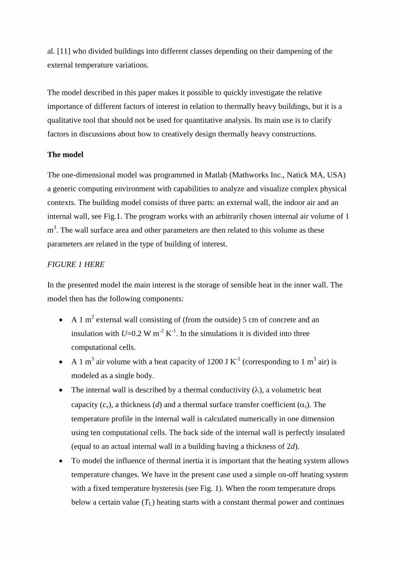
al. [11] who divided buildings into different classes depending on their dampening of the

external temperature variations.

The model described in this paper makes it possible to quickly investigate the relative

importance of different factors of interest in relation to thermally heavy buildings, but it is a

qualitative tool that should not be used for quantitative analysis. Its main use is to clarify

factors in discussions about how to creatively design thermally heavy constructions.

The model

The one-dimensional model was programmed in Matlab (Mathworks Inc., Natick MA, USA)

a generic computing environment with capabilities to analyze and visualize complex physical

contexts. The building model consists of three parts: an external wall, the indoor air and an

internal wall, see Fig.1. The program works with an arbitrarily chosen internal air volume of 1

m3. The wall surface area and other parameters are then related to this volume as these

parameters are related in the type of building of interest.

FIGURE 1 HERE

In the presented model the main interest is the storage of sensible heat in the inner wall. The

model then has the following components:

A 1 m2 external wall consisting of (from the outside) 5 cm of concrete and an

insulation with U=0.2 W m-2

K-1

. In the simulations it is divided into three

computational cells.

A 1 m3 air volume with a heat capacity of 1200 J K

-1 (corresponding to 1 m

3 air) is

modeled as a single body.

The internal wall is described by a thermal conductivity (), a volumetric heat

capacity (cv), a thickness (d) and a thermal surface transfer coefficient (i). The

temperature profile in the internal wall is calculated numerically in one dimension

using ten computational cells. The back side of the internal wall is perfectly insulated

(equal to an actual internal wall in a building having a thickness of 2d).

To model the influence of thermal inertia it is important that the heating system allows

temperature changes. We have in the present case used a simple on-off heating system

with a fixed temperature hysteresis (see Fig. 1). When the room temperature drops

below a certain value (TL) heating starts with a constant thermal power and continues

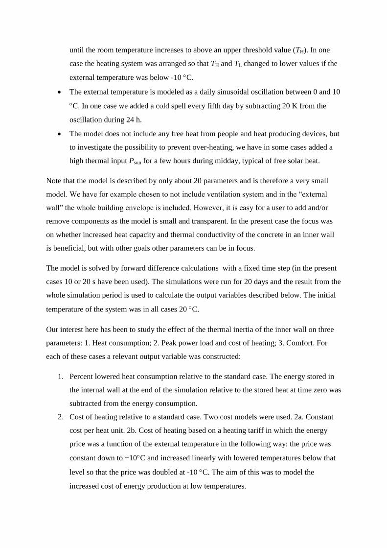
until the room temperature increases to above an upper threshold value (TH). In one

case the heating system was arranged so that TH and TL changed to lower values if the

external temperature was below -10 C.

The external temperature is modeled as a daily sinusoidal oscillation between 0 and 10

C. In one case we added a cold spell every fifth day by subtracting 20 K from the

oscillation during 24 h.

The model does not include any free heat from people and heat producing devices, but

to investigate the possibility to prevent over-heating, we have in some cases added a

high thermal input Psun for a few hours during midday, typical of free solar heat.

Note that the model is described by only about 20 parameters and is therefore a very small

model. We have for example chosen to not include ventilation system and in the “external

wall” the whole building envelope is included. However, it is easy for a user to add and/or

remove components as the model is small and transparent. In the present case the focus was

on whether increased heat capacity and thermal conductivity of the concrete in an inner wall

is beneficial, but with other goals other parameters can be in focus.

The model is solved by forward difference calculations with a fixed time step (in the present

cases 10 or 20 s have been used). The simulations were run for 20 days and the result from the

whole simulation period is used to calculate the output variables described below. The initial

temperature of the system was in all cases 20 C.

Our interest here has been to study the effect of the thermal inertia of the inner wall on three

parameters: 1. Heat consumption; 2. Peak power load and cost of heating; 3. Comfort. For

each of these cases a relevant output variable was constructed:

1. Percent lowered heat consumption relative to the standard case. The energy stored in

the internal wall at the end of the simulation relative to the stored heat at time zero was

subtracted from the energy consumption.

2. Cost of heating relative to a standard case. Two cost models were used. 2a. Constant

cost per heat unit. 2b. Cost of heating based on a heating tariff in which the energy

price was a function of the external temperature in the following way: the price was

constant down to +10C and increased linearly with lowered temperatures below that

level so that the price was doubled at -10 C. The aim of this was to model the

increased cost of energy production at low temperatures.

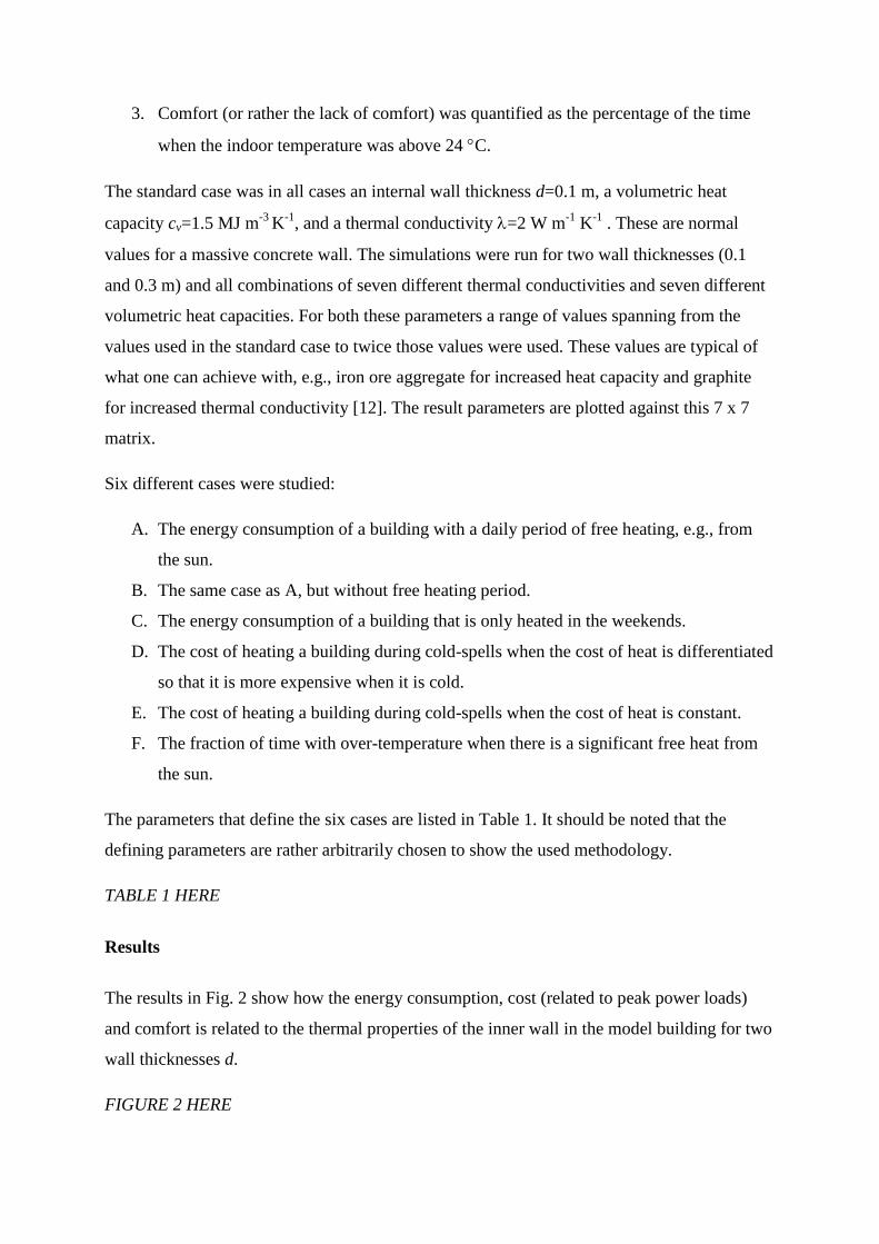
3. Comfort (or rather the lack of comfort) was quantified as the percentage of the time

when the indoor temperature was above 24 C.

The standard case was in all cases an internal wall thickness d=0.1 m, a volumetric heat

capacity cv=1.5 MJ m-3

K-1

, and a thermal conductivity =2 W m-1

K-1

. These are normal

values for a massive concrete wall. The simulations were run for two wall thicknesses (0.1

and 0.3 m) and all combinations of seven different thermal conductivities and seven different

volumetric heat capacities. For both these parameters a range of values spanning from the

values used in the standard case to twice those values were used. These values are typical of

what one can achieve with, e.g., iron ore aggregate for increased heat capacity and graphite

for increased thermal conductivity [12]. The result parameters are plotted against this 7 x 7

matrix.

Six different cases were studied:

A. The energy consumption of a building with a daily period of free heating, e.g., from

the sun.

B. The same case as A, but without free heating period.

C. The energy consumption of a building that is only heated in the weekends.

D. The cost of heating a building during cold-spells when the cost of heat is differentiated

so that it is more expensive when it is cold.

E. The cost of heating a building during cold-spells when the cost of heat is constant.

F. The fraction of time with over-temperature when there is a significant free heat from

the sun.

The parameters that define the six cases are listed in Table 1. It should be noted that the

defining parameters are rather arbitrarily chosen to show the used methodology.

TABLE 1 HERE

Results

The results in Fig. 2 show how the energy consumption, cost (related to peak power loads)

and comfort is related to the thermal properties of the inner wall in the model building for two

wall thicknesses d.

FIGURE 2 HERE

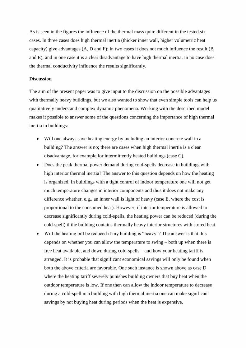
As is seen in the figures the influence of the thermal mass quite different in the tested six

cases. In three cases does high thermal inertia (thicker inner wall, higher volumetric heat

capacity) give advantages (A, D and F); in two cases it does not much influence the result (B

and E); and in one case it is a clear disadvantage to have high thermal inertia. In no case does

the thermal conductivity influence the results significantly.

Discussion

The aim of the present paper was to give input to the discussion on the possible advantages

with thermally heavy buildings, but we also wanted to show that even simple tools can help us

qualitatively understand complex dynamic phenomena. Working with the described model

makes it possible to answer some of the questions concerning the importance of high thermal

inertia in buildings:

Will one always save heating energy by including an interior concrete wall in a

building? The answer is no; there are cases when high thermal inertia is a clear

disadvantage, for example for intermittently heated buildings (case C).

Does the peak thermal power demand during cold-spells decrease in buildings with

high interior thermal inertia? The answer to this question depends on how the heating

is organized. In buildings with a tight control of indoor temperature one will not get

much temperature changes in interior components and thus it does not make any

difference whether, e.g., an inner wall is light of heavy (case E, where the cost is

proportional to the consumed heat). However, if interior temperature is allowed to

decrease significantly during cold-spells, the heating power can be reduced (during the

cold-spell) if the building contains thermally heavy interior structures with stored heat.

Will the heating bill be reduced if my building is “heavy”? The answer is that this

depends on whether you can allow the temperature to swing – both up when there is

free heat available, and down during cold-spells – and how your heating tariff is

arranged. It is probable that significant economical savings will only be found when

both the above criteria are favorable. One such instance is shown above as case D

where the heating tariff severely punishes building owners that buy heat when the

outdoor temperature is low. If one then can allow the indoor temperature to decrease

during a cold-spell in a building with high thermal inertia one can make significant

savings by not buying heat during periods when the heat is expensive.

Is the thermal indoor climate better in buildings with high thermal inertia? This

question is complex as even if it is true that the temperature variations will be lower in

a thermally heavy building (case F) – all other parameters the same – this will also

decrease temperature variations and thus the possibility of making savings on the

heating and the peak powers.

It is obvious that a high volumetric heat capacity leads to high thermal inertia, but is it

important to also have a high thermal conductivity in the heavy construction part? In

the present simulations the thermal conductivity did not matter very much is it is in all

cases high enough to give rather small temperature gradients in the inner wall during

the daily temperature variations.

These general results concerning the influence of thermal mass agree with what has been

found in previous studies. For example did Bloomfield and Fisk [13] in a study on daily

intermittent heating (decreasing heating when a building like an office is not used) conclude

that the additional thermal inertia of heavy-weight buildings do not offer any substantial

energy savings in the case of intermittent heating (although an intermittent heating strategy

needs to be tailored to the thermal inertia of the building [13-14]). What one gains by not

heating in one period is approximately lost when one has to heat more before people enter the

building. It is thus not obvious that one will, e.g., save energy by increasing the thermal mass

of a building. Statements like “The thermal mass of concrete in buildings […] Reduces

heating energy consumption by 2 – 15%” [15] are not generally true. If positive effects can be

achieved depend on many factors, like climatic conditions and acceptable indoor

requirements, and it may be difficult to get only positive benefits from a high thermal mass;

cf. Shao [8] who points out that “high thermal mass design could introduce conflicting

requirements for winter heating and summer cooling”.

Bellamy and Mackenzie [16] studied two test houses that were identical except for that one of

the houses had a high thermal mass inside the external insulation. In their case the energy

savings in a continuously heated house were strongly related to the reduction in ventilation

requirements for cooling provided by heavy walls. They point out that “[s]imply replacing

lightweight walls with heavy walls of equivalent R-value may increase or decrease the

auxiliary heating requirements depending on the house design, climate and occupant

behavior”. Bellamy and Mackenzie [16] also found that the heavy building had significantly

less over-heating, giving it a better indoor environment.

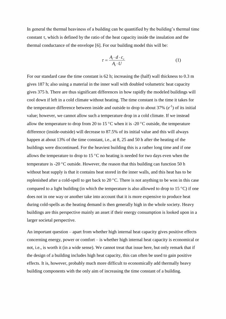
In general the thermal heaviness of a building can be quantified by the building’s thermal time

constant , which is defined by the ratio of the heat capacity inside the insulation and the

thermal conductance of the envelope [6]. For our building model this will be:

UA

cdA

e

vi

(1)

For our standard case the time constant is 62 h; increasing the (half) wall thickness to 0.3 m

gives 187 h; also using a material in the inner wall with doubled volumetric heat capacity

gives 375 h. There are thus significant differences in how rapidly the modeled buildings will

cool down if left in a cold climate without heating. The time constant is the time it takes for

the temperature difference between inside and outside to drop to about 37% (e-1

) of its initial

value; however, we cannot allow such a temperature drop in a cold climate. If we instead

allow the temperature to drop from 20 to 15 C when it is -20 C outside, the temperature

difference (inside-outside) will decrease to 87.5% of its initial value and this will always

happen at about 13% of the time constant, i.e., at 8, 25 and 50 h after the heating of the

buildings were discontinued. For the heaviest building this is a rather long time and if one

allows the temperature to drop to 15 C no heating is needed for two days even when the

temperature is -20 C outside. However, the reason that this building can function 50 h

without heat supply is that it contains heat stored in the inner walls, and this heat has to be

replenished after a cold-spell to get back to 20 C. There is not anything to be won in this case

compared to a light building (in which the temperature is also allowed to drop to 15 C) if one

does not in one way or another take into account that it is more expensive to produce heat

during cold-spells as the heating demand is then generally high in the whole society. Heavy

buildings are this perspective mainly an asset if their energy consumption is looked upon in a

larger societal perspective.

An important question – apart from whether high internal heat capacity gives positive effects

concerning energy, power or comfort – is whether high internal heat capacity is economical or

not, i.e., is worth it (in a wide sense). We cannot treat that issue here, but only remark that if

the design of a building includes high heat capacity, this can often be used to gain positive

effects. It is, however, probably much more difficult to economically add thermally heavy

building components with the only aim of increasing the time constant of a building.

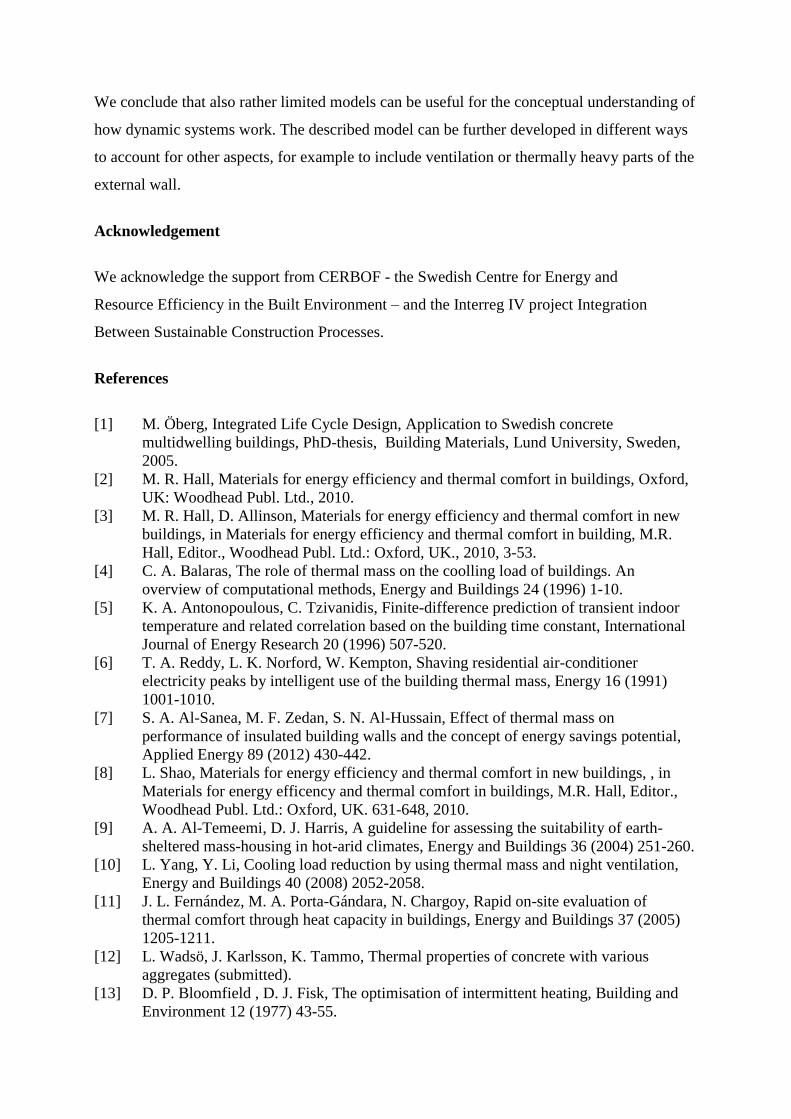
We conclude that also rather limited models can be useful for the conceptual understanding of

how dynamic systems work. The described model can be further developed in different ways

to account for other aspects, for example to include ventilation or thermally heavy parts of the

external wall.

Acknowledgement

We acknowledge the support from CERBOF - the Swedish Centre for Energy and

Resource Efficiency in the Built Environment – and the Interreg IV project Integration

Between Sustainable Construction Processes.

References

[1] M. Öberg, Integrated Life Cycle Design, Application to Swedish concrete

multidwelling buildings, PhD-thesis, Building Materials, Lund University, Sweden,

2005.

[2] M. R. Hall, Materials for energy efficiency and thermal comfort in buildings, Oxford,

UK: Woodhead Publ. Ltd., 2010.

[3] M. R. Hall, D. Allinson, Materials for energy efficiency and thermal comfort in new

buildings, in Materials for energy efficiency and thermal comfort in building, M.R.

Hall, Editor., Woodhead Publ. Ltd.: Oxford, UK., 2010, 3-53.

[4] C. A. Balaras, The role of thermal mass on the coolling load of buildings. An

overview of computational methods, Energy and Buildings 24 (1996) 1-10.

[5] K. A. Antonopoulous, C. Tzivanidis, Finite-difference prediction of transient indoor

temperature and related correlation based on the building time constant, International

Journal of Energy Research 20 (1996) 507-520.

[6] T. A. Reddy, L. K. Norford, W. Kempton, Shaving residential air-conditioner

electricity peaks by intelligent use of the building thermal mass, Energy 16 (1991)

1001-1010.

[7] S. A. Al-Sanea, M. F. Zedan, S. N. Al-Hussain, Effect of thermal mass on

performance of insulated building walls and the concept of energy savings potential,

Applied Energy 89 (2012) 430-442.

[8] L. Shao, Materials for energy efficiency and thermal comfort in new buildings, , in

Materials for energy efficency and thermal comfort in buildings, M.R. Hall, Editor.,

Woodhead Publ. Ltd.: Oxford, UK. 631-648, 2010.

[9] A. A. Al-Temeemi, D. J. Harris, A guideline for assessing the suitability of earth-

sheltered mass-housing in hot-arid climates, Energy and Buildings 36 (2004) 251-260.

[10] L. Yang, Y. Li, Cooling load reduction by using thermal mass and night ventilation,

Energy and Buildings 40 (2008) 2052-2058.

[11] J. L. Fernández, M. A. Porta-Gándara, N. Chargoy, Rapid on-site evaluation of

thermal comfort through heat capacity in buildings, Energy and Buildings 37 (2005)

1205-1211.

[12] L. Wadsö, J. Karlsson, K. Tammo, Thermal properties of concrete with various

aggregates (submitted).

[13] D. P. Bloomfield , D. J. Fisk, The optimisation of intermittent heating, Building and

Environment 12 (1977) 43-55.

[14] D. Pupeikis, A. Burlingis, V. Stankeičius, Required additional heating power of

building during intermitted heating, Journal or Civil Engineering and Management 16

(2010) 141-148.

[15] Anon., Concrete for energy efficient buildings. The benefits of thermal mass, in

http://www.efca.info/downloads/Concrete_for%20Energy_Efficient_Buildings.pdf,

E.C.P. ASBL, Editor. 2007.

[16] L. A. Bellamy , D. W. Mackenzie, Thermal performance of buildings with heavy

walls, Study Report 108, BRANZ, New Zealand, 2001.

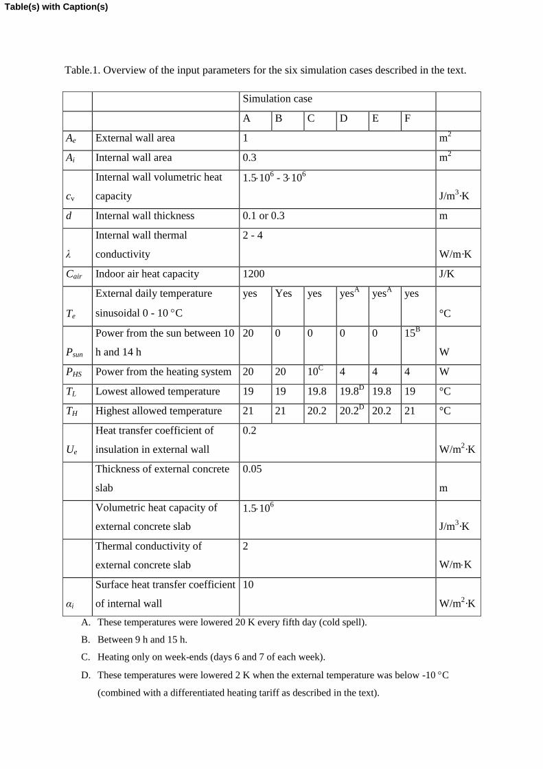
Table.1. Overview of the input parameters for the six simulation cases described in the text.

Simulation case

A B C D E F

Ae External wall area 1 m2

Ai Internal wall area 0.3 m2

cv

Internal wall volumetric heat

capacity

1.5106 - 310

6

J/m3·K

d Internal wall thickness 0.1 or 0.3 m

λ

Internal wall thermal

conductivity

2 - 4

W/m·K

Cair Indoor air heat capacity 1200 J/K

Te

External daily temperature

sinusoidal 0 - 10 C

yes Yes yes

yesA yes

A yes

°C

Psun

Power from the sun between 10

h and 14 h

20 0 0 0

0 15B

W

PHS Power from the heating system 20 20 10C

4 4 4 W

TL Lowest allowed temperature 19 19 19.8 19.8D 19.8 19 °C

TH Highest allowed temperature 21 21 20.2 20.2D 20.2 21 °C

Ue

Heat transfer coefficient of

insulation in external wall

0.2

W/m2·K

Thickness of external concrete

slab

0.05

m

Volumetric heat capacity of

external concrete slab

1.5106

J/m3·K

Thermal conductivity of

external concrete slab

2

W/mK

αi

Surface heat transfer coefficient

of internal wall

10

W/m2·K

A. These temperatures were lowered 20 K every fifth day (cold spell).

B. Between 9 h and 15 h.

C. Heating only on week-ends (days 6 and 7 of each week).

D. These temperatures were lowered 2 K when the external temperature was below -10 C

(combined with a differentiated heating tariff as described in the text).

Table(s) with Caption(s)

Figure captions

Figure 1. Overview of the variables in the model.

Figure 2. The simulated results in the six cases described in Table 1 and the text. The top

surface in each diagram is for a wall thickness of 0.1 m and the lower surface is for a wall

thickness of 0.3 m (for Fig. B and E only one surface is shown as the two surfaces are almost

identical). Note that the plots have been rotated differently in the heat capacity – thermal

conductivity plane to more clearly show each result. The coloring differentiates different

levels.

List of Figure Captions

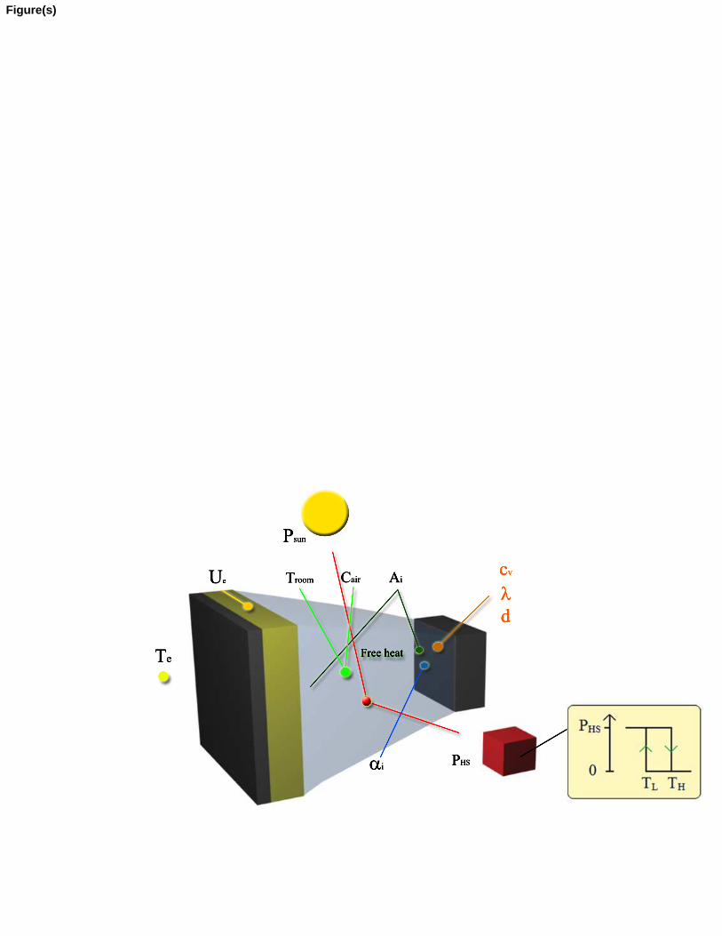
Figure(s)

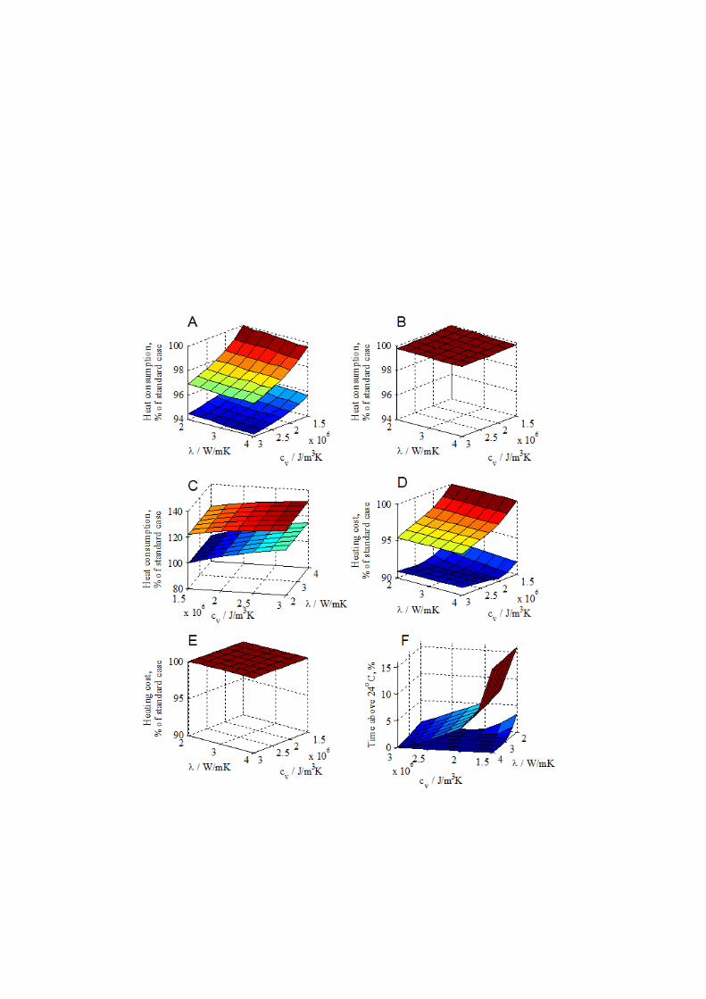
PAPERIIIL. Wadsö, J. Karlsson and K. Tammo “Thermal properties of concrete with various aggregates” (submitted to Cement and Concrete Research).

III

LW 3 April 2012

Thermal properties of concrete with various aggregates

L. Wadsöa,c , J. Karlssona and K. Tammob

a Building Materials, Lund University, Box 118, 221 00 Lund, Sweden

b The Swedish Cement and Concrete Research Institute (CBI), Box 118 Lund, Sweden

c Corresponding author

ABSTRACT

The thermal mass of buildings can influence heat consumption, peak powers, and thermal

comfort. Concrete is the most common building material with a high thermal mass. We have

studied whether it is possible to improve the thermal properties of concrete by using

aggregates with high heat capacity and/or materials with high thermal conductivity. It was

found that both volumetric heat capacity and thermal conductivity could be simple means be

increased by at least 50% compared to standards concrete.

INTRODUCTION

The thermal properties of building materials are of importance for the designer of energy

efficient buildings. This includes light insulating materials that can be used to reduce the heat

losses through the building envelope, but to some extent also materials with high thermal

inertia that can store heat and delay the conduction of heat through structural elements. The

most common example of the latter type of material is concrete that is widely used in the

building sector to make for example slabs on the ground, walls (both precast, cast on site and

in the form of concrete building blocks), floors (both precast and cast on site), and roof tiles.

In all these applications the thermal properties of the concrete will influence the performance

of the building. For example will the efficiency of cast-in flooring systems depend on the

thermal properties of concrete, concrete roof tiles will to some extent buffer day-time solar

radiation and night-time heat losses, and all concrete structures inside the insulation of the

building envelope will decrease indoor temperature variations. Thermally heavy structures

inside the building envelope may be of significant relevance in a future more energy efficient

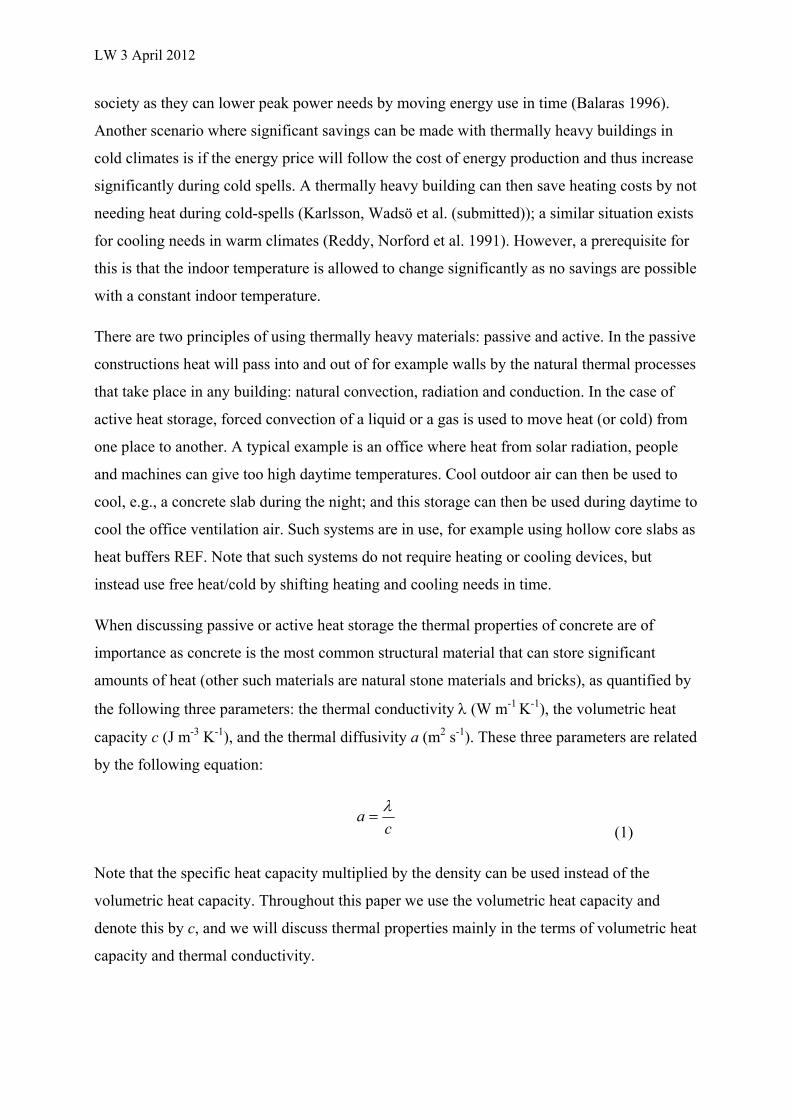
LW 3 April 2012

society as they can lower peak power needs by moving energy use in time (Balaras 1996).

Another scenario where significant savings can be made with thermally heavy buildings in

cold climates is if the energy price will follow the cost of energy production and thus increase

significantly during cold spells. A thermally heavy building can then save heating costs by not

needing heat during cold-spells (Karlsson, Wadsö et al. (submitted)); a similar situation exists

for cooling needs in warm climates (Reddy, Norford et al. 1991). However, a prerequisite for

this is that the indoor temperature is allowed to change significantly as no savings are possible

with a constant indoor temperature.

There are two principles of using thermally heavy materials: passive and active. In the passive

constructions heat will pass into and out of for example walls by the natural thermal processes

that take place in any building: natural convection, radiation and conduction. In the case of

active heat storage, forced convection of a liquid or a gas is used to move heat (or cold) from

one place to another. A typical example is an office where heat from solar radiation, people

and machines can give too high daytime temperatures. Cool outdoor air can then be used to

cool, e.g., a concrete slab during the night; and this storage can then be used during daytime to

cool the office ventilation air. Such systems are in use, for example using hollow core slabs as

heat buffers REF. Note that such systems do not require heating or cooling devices, but

instead use free heat/cold by shifting heating and cooling needs in time.

When discussing passive or active heat storage the thermal properties of concrete are of

importance as concrete is the most common structural material that can store significant

amounts of heat (other such materials are natural stone materials and bricks), as quantified by

the following three parameters: the thermal conductivity (W m-1 K-1), the volumetric heat

capacity c (J m-3 K-1), and the thermal diffusivity a (m2 s-1). These three parameters are related

by the following equation:

c

a

(1)

Note that the specific heat capacity multiplied by the density can be used instead of the

volumetric heat capacity. Throughout this paper we use the volumetric heat capacity and

denote this by c, and we will discuss thermal properties mainly in the terms of volumetric heat

capacity and thermal conductivity.

LW 3 April 2012

Of the two parameters heat capacity and thermal conductivity, it is the heat capacity that is

most important for high thermal inertia components in buildings. If the volumetric heat

capacity of a concrete member is increased by 50%, 50% more heat can be stored in this

construction part. At least for temperature variations on the time scale of the order of a day,

nearly the whole thickness of standard concrete walls will follow the room temperature

variations so an increased thermal conductivity in normally not an asset in this case. This can

be illustrated by the following figures. Standard concrete has an approximate thermal

diffusivity of 10-6 m2 s-1. If a concrete wall with a homogeneous temperature distribution is

exposed to the same temperature change on both its surfaces, the time it takes for 90% of the

heat to flow in or out of the wall to achieve a new stationary condition is 40 min, 2.5 h and 10

h for walls with thicknesses 10 cm, 20 cm and 40 cm (in the absence of surface mass transfer

resistances like boundary layers or wall papers). However, the situation may be different

when quick heat storage is important; for example to take care of intensive free solar heat

during a few hours.

Concrete is a composite material and its thermal properties are a function of the thermal

properties, volume fractions and morphology of its constituents (phases): cement paste, air

(pores), fine aggregate (sand), and large aggregates (rock material). The thermal properties of

a cement paste – including fine (gel and capillary) pores – depend on the water/cement-ratio,

the degree of hydration and the moisture content. In well hydrated and air-dried concrete the

thermal properties are mainly functions of the water/cement-ratio (w/c) as higher such ratios

give a more porous structure. Typical thermal conductance values for OPC (ordinary Portland

cement) pastes in the literature are between 0.5 W m-1 K-1 for w/c=0.5 (Valore 1980) to 1.0

for w/c=0.3-0.4 (Bentz 2007). Volumetric heat capacities are strongly dependent on the water

content as both chemically bound, physically bound and free water has a high heat capacity.

Liquid water has a specific heat capacity of about 4200 J kg-1 K-1 and bound water in cement

hydrates has a specific heat capacity of about 2200 J kg-1 K-1 (Bentz 2007) (similar to that of

ice). The specific heat capacity of a seal cured w/c=0.4 OPC cement paste with a degree of

hydration of 0.8 is approx. 1400 J kg-1 K-1 (Bentz 2007). With a density of air dried w/c=0.5

cement paste of about 1480 kg m-3 (Lamond and Pielert 2006) we get a volumetric heat

capacity of approx. 2.1 MJ m-3 K-1. However, this value is very dependent on the moisture

content.

The larger pores – usually 2-4% of a concrete - have such a low thermal conductivity and heat

capacity compared to the other phases (if they are filled with air) that the values of both these

LW 3 April 2012

properties can in practice be assumed to be zero. If the pores are partially or fully filled with

water – something that will happen in for example outdoor applications or in concrete in

contact with the ground – both thermal conductivity and heat capacity will be increased.

Sand and larger aggregates are normally natural minerals with different thermal properties.

However, from a practical point of view, most minerals and rocks used as aggregates have

similar thermal properties except that quartz and quartz based rocks that have a significantly

higher thermal conductivity (cf. Fig. 1D in (Clauser and Huenges 1995)). It is thus of

importance to know how much quartz the aggregate contains to be able to make calculations

of thermal properties of sand, aggregate and concrete.

For special applications other types of concrete aggregates with quite different thermal

properties can be used. For example can insulating expanded clay particles be used as

aggregate to make a more insulating concrete. A new type of aggregate is phase change

materials (PCMs) that will consume heat by melting in a rather narrow temperature range; this

can be seen as that the material has an extremely high heat capacity in a limited temperature

interval. Such materials are commonly made from paraffin and have been investigated also

for use in concrete (Bentz and Turpin 2007; Hunger, Entrop et al. 2009).

Thermal properties of composite materials are of significant interest in many fields. Some

examples are thermal properties of rock materials (Horai and Simmons 1969; Clauser and

Huenges 1995) and polymers (Weidenfeller, Höfer et al. 2004). There have also been

presented several studies of thermal properties of concrete. For example did Marshall

(Marshall 1972) give an overview of the work done up to 1972. Valore (Valore 1980)

discussed thermal conductivity of mortars and concrete to be used for the calculations of U-

values of walls, including the influence of moisture content and type of aggregate. His

methods and values have later been used in a design guide report issued by the American

Concrete Institute (Cavanaugh 2002). Khan (Khan 2002) measured thermal conductivity on

concretes with different aggregates and found that the thermal conductivity was about 35%

higher when the large aggregate was quartz-based, than when it was based on basalt,

limestone and siltstone. He also found that the moisture content of the concrete had a

significant influence on the thermal conductivity of concrete; for a quartzite concrete the

thermal conductivity increased from 2.7 to 4 W m-1 K-1 when the moisture content increased

from zero to 7.5%. Kim et al. (Kim, Jeon et al. 2003) studied the thermal conductivity of

concrete as a function of aggregate fraction, water/cement-ratio, temperature and humidity.

LW 3 April 2012

Bentz et al. (Bentz, Peltz et al. 2011) measured the thermal properties of fly ash concretes.

They found that for well hydrated concretes the law of mixtures gave a reasonable prediction

of the thermal properties. Thermal conductivity was strongly influenced by whether the

aggregate contained quartz. Several fire-related studies have also been made on high

temperature properties of concrete (see for example reference (Kodur and Sultan 2003)).

The aim of the present study was to investigate how the thermal properties of concrete inside

the building envelope could be changed in the direction of higher thermal conductivity and/or

higher heat capacity by the use of different aggregates. Eleven different concretes were cast

and their thermal properties were investigated with a TPS (Transient Plane Source) technique.

We also compare our results with approximate calculations using the mixing model

(volumetric heat capacity) and the Hashin-Shtrikman model (thermal conductivity).

METHODS

We used transient plane source (TPS) measurements to measure volumetric heat capacity and

thermal conductivity of concretes and aggregates. For the TPS-measurements (Gustafsson

1991) we use a HotDisk 1500 (HotDisk AB, Göteborg, Sweden) in the single side mode using

an extruded polystyrene (=0.032 W m-1 K-1; c=0.5 MJ m-3 K-1) on the other side. As

concretes are inhomogeneous materials we used the largest available sensor (number 5599)

with a diameter of almost 57 mm for the concrete measurements. This is about 3.6 times the

diameter of the largest aggregate of the concrete composite structures. For aggregate

measurements we used smaller sensors; for the magnetite measurements – where we only had

30 mm diameter samples, we used a 5501 sensor with a 12.8 mm diameter.

The cast blocks were water cut after 28 days and thereafter stored in room climate. Before the

measurements the used surfaces were made plane with a diamond (dry).

The HotDisk measurement time for the concrete measurements was about 160 s and the

thermal power was about 0.5 W. For each material, at least three measurements were made in

each of three areas on a sample. The non-PCM concretes were measured at about 24 C, while

the PCM containing concretes were measured at 5 and 50 C as the HotDisk method does not

work if the studied materials melt in the temperature range of a measurement. Measurements

were thus conducted both below and above the phase change temperatures of the PCMs. Note

that the phase changes were not studied.

MATERIALS

LW 3 April 2012

We used eleven different concretes: one reference, seven with aggregate with high heat

capacity and/or high thermal conductivity, and three concretes with phase change materials

(PCM). The recipes are given in Table 1 together with details on the used materials. Note that

none of the PCM products used are normally used in concrete.

The concretes were mixed in a free fall mixer, cast in 150 mm steel cube forms, demoulded

after about 1 day, and hydrated for 28 days in water. At the time of the HotDisk

measurements the specimens had been stored for about a year in indoor conditions. Their

relative humidity (measured on four random samples) was 30-40%, which is in the range that

indoor concrete will have in cold climates or exterior protected concrete in warm climates.

The materials used were as follows.

Reference concrete (REF)

This is a standard concrete with a water/cement-ratio of 0.5 and a cement content of 381 kg

m-3. The fine aggregate was 0-8 mm sand of mixed composition (quartz and other minerals);

the large aggregate was quartzite.

Magnetite concrete (MAG)

This concrete is similar to REF, but with less fine aggregate and with magnetite (iron ore) as

large aggregate. Magnetite has a high density and a high volumetric heat capacity.

Graphite concrete (GRA)

This concrete has a significantly higher cement content (533 kg m-3) and higher water/cement-

ratio (0.59) than REF, and also contains expandable graphite that has a high thermal

conductivity. Expandable graphite is produced from natural graphite by introducing sulfur or

nitrogen atoms between the carbon layers. When it is exposed to high temperature expandable

graphite will expand up to a hundred times and it can therefore be used, e.g., as a high

temperature fire protection. The expandable graphite used here was not expanded, and is here

assumed to have similar properties as natural graphite.

Graphite and magnetite concrete (GAM)

This concrete is a combination of MAG and GRA with water/cement-ratio 0.60.

Steel fiber concrete (ST1)

LW 3 April 2012

This is similar to REF, but also contains 100 kg m-3 of steel fibers.

Steel fiber concrete with high concentration of fibers (ST2)

Similar to ST1, but with 197 kg m-3 of steel fibers.

Concrete with brass shavings (BRA)

Similar to REF, but with an addition of 5%(vol) of brass shavings that have a high thermal

conductivity.

Concrete with copper wires (COP)

Similar to REF, but with an addition of 2.5%(vol) of copper wires that have a very high

thermal conductivity.

Concrete with PCM pellets (PEL)

This micro-concrete had a water/cement-ratio of 0.5 and did not contain any large aggregate,

but an addition of a macro-encapsulated phased change material (PCM) product with the size

of rice grains.

Concrete with micro PCM (MIC)

This micro-concrete had a high water/cement-ratio and did not contain any large aggregate,

but an addition of micro-encapsulated PCM particles with a diameter of less than 0.5 mm.

Concrete with PCM dispersion (DIS)

This concrete had an addition of a PCM dispersion product.

Cement paste (PAS)

A water/cement-ratio 0.5 cement paste was also included to get values of the heat capacity

and thermal conductivity of the cement paste.

Of the above materials, only REF, MAG, ST1, ST2, BRA and COP had normal cube

strengths. The macro-encapsulated PCMs in the PEL concrete expanded out of the specimens

when they were heated, and the DIS sample had to be handled with care as it would easily

break (none of the PCM products are produced for use in concrete).

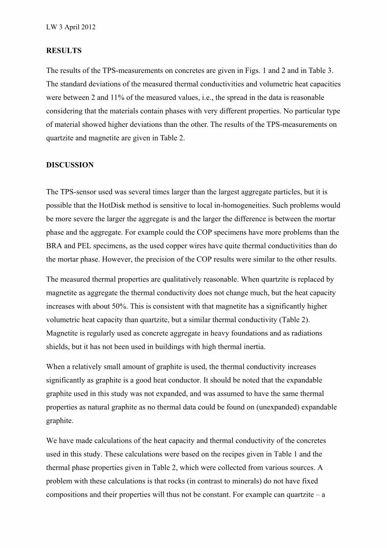
LW 3 April 2012

RESULTS

The results of the TPS-measurements on concretes are given in Figs. 1 and 2 and in Table 3.

The standard deviations of the measured thermal conductivities and volumetric heat capacities

were between 2 and 11% of the measured values, i.e., the spread in the data is reasonable

considering that the materials contain phases with very different properties. No particular type

of material showed higher deviations than the other. The results of the TPS-measurements on

quartzite and magnetite are given in Table 2.

DISCUSSION

The TPS-sensor used was several times larger than the largest aggregate particles, but it is

possible that the HotDisk method is sensitive to local in-homogeneities. Such problems would

be more severe the larger the aggregate is and the larger the difference is between the mortar

phase and the aggregate. For example could the COP specimens have more problems than the

BRA and PEL specimens, as the used copper wires have quite thermal conductivities than do

the mortar phase. However, the precision of the COP results were similar to the other results.

The measured thermal properties are qualitatively reasonable. When quartzite is replaced by

magnetite as aggregate the thermal conductivity does not change much, but the heat capacity

increases with about 50%. This is consistent with that magnetite has a significantly higher

volumetric heat capacity than quartzite, but a similar thermal conductivity (Table 2).

Magnetite is regularly used as concrete aggregate in heavy foundations and as radiations

shields, but it has not been used in buildings with high thermal inertia.

When a relatively small amount of graphite is used, the thermal conductivity increases

significantly as graphite is a good heat conductor. It should be noted that the expandable

graphite used in this study was not expanded, and was assumed to have the same thermal

properties as natural graphite as no thermal data could be found on (unexpanded) expandable

graphite.

We have made calculations of the heat capacity and thermal conductivity of the concretes

used in this study. These calculations were based on the recipes given in Table 1 and the

thermal phase properties given in Table 2, which were collected from various sources. A

problem with these calculations is that rocks (in contrast to minerals) do not have fixed

compositions and their properties will thus not be constant. For example can quartzite – a

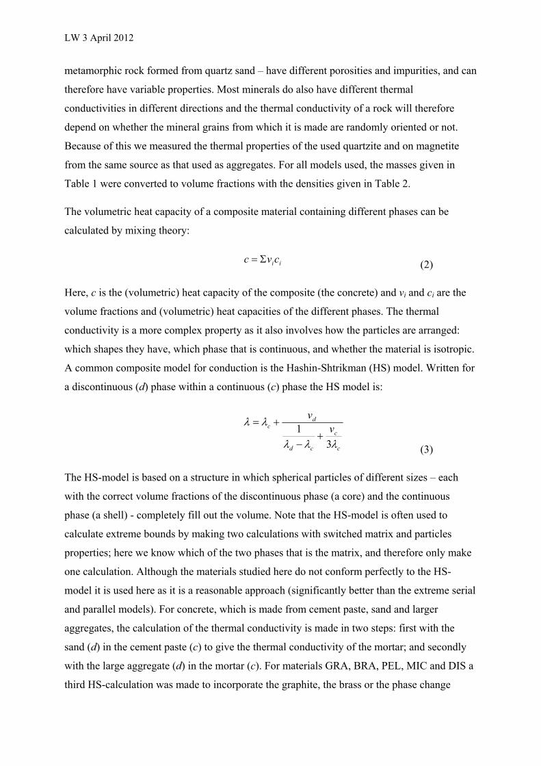
LW 3 April 2012

metamorphic rock formed from quartz sand – have different porosities and impurities, and can

therefore have variable properties. Most minerals do also have different thermal

conductivities in different directions and the thermal conductivity of a rock will therefore

depend on whether the mineral grains from which it is made are randomly oriented or not.

Because of this we measured the thermal properties of the used quartzite and on magnetite

from the same source as that used as aggregates. For all models used, the masses given in

Table 1 were converted to volume fractions with the densities given in Table 2.

The volumetric heat capacity of a composite material containing different phases can be

calculated by mixing theory:

iicvc (2)

Here, c is the (volumetric) heat capacity of the composite (the concrete) and vi and ci are the

volume fractions and (volumetric) heat capacities of the different phases. The thermal

conductivity is a more complex property as it also involves how the particles are arranged:

which shapes they have, which phase that is continuous, and whether the material is isotropic.

A common composite model for conduction is the Hashin-Shtrikman (HS) model. Written for

a discontinuous (d) phase within a continuous (c) phase the HS model is:

c

c

cd

dc v

v

3

1

(3)

The HS-model is based on a structure in which spherical particles of different sizes – each

with the correct volume fractions of the discontinuous phase (a core) and the continuous

phase (a shell) - completely fill out the volume. Note that the HS-model is often used to

calculate extreme bounds by making two calculations with switched matrix and particles

properties; here we know which of the two phases that is the matrix, and therefore only make

one calculation. Although the materials studied here do not conform perfectly to the HS-

model it is used here as it is a reasonable approach (significantly better than the extreme serial

and parallel models). For concrete, which is made from cement paste, sand and larger

aggregates, the calculation of the thermal conductivity is made in two steps: first with the

sand (d) in the cement paste (c) to give the thermal conductivity of the mortar; and secondly

with the large aggregate (d) in the mortar (c). For materials GRA, BRA, PEL, MIC and DIS a

third HS-calculation was made to incorporate the graphite, the brass or the phase change

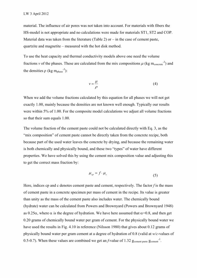
LW 3 April 2012

material. The influence of air pores was not taken into account. For materials with fibers the

HS-model is not appropriate and no calculations were made for materials ST1, ST2 and COP.

Material data was taken from the literature (Table 2) or – in the case of cement paste,

quartzite and magnetite – measured with the hot disk method.

To use the heat capacity and thermal conductivity models above one need the volume

fractions v of the phases. These are calculated from the mix compositions (kg mconcrete-3) and

the densities (kg mphase-3):

v (4)

When we add the volume fractions calculated by this equation for all phases we will not get

exactly 1.00, mainly because the densities are not known well enough. Typically our results

were within 5% of 1.00. For the composite model calculations we adjust all volume fractions

so that their sum equals 1.00.

The volume fraction of the cement paste could not be calculated directly with Eq. 3, as the

“mix composition” of cement paste cannot be directly taken from the concrete recipe, both

because part of the used water leaves the concrete by drying, and because the remaining water

is both chemically and physically bound, and these two “types” of water have different

properties. We have solved this by using the cement mix composition value and adjusting this

to get the correct mass fraction by:

ccp f (5)

Here, indices cp and c denotes cement paste and cement, respectively. The factor f is the mass

of cement paste in a concrete specimen per mass of cement in the recipe. Its value is greater

than unity as the mass of the cement paste also includes water. The chemically bound

(hydrate) water can be calculated from Powers and Brownyard (Powers and Brownyard 1948)

as 0.25, where is the degree of hydration. We have here assumed that =0.8, and then get

0.20 grams of chemically bound water per gram of cement. For the physically bound water we

have used the results in Fig. 4.10 in reference (Nilsson 1980) that gives about 0.12 grams of

physically bound water per gram cement at a degree of hydration of 0.8 (valid at w/c-values of

0.5-0.7). When these values are combined we get an f-value of 1.32 gcement paste gcement-1.

LW 3 April 2012

The results from measurements and calculations are given in Table 3. It is seen that the

calculations show a fair agreement with the measured data in most cases; and that the results

are good enough for engineering calculations of thermal storage in construction details for

these cases. Two materials for which the HS-model did not calculate the correct thermal

conductivity value is GRA and GAM. This mismatch between measurement and calculation is

most probably because the anisotropic graphite particles are arranged as flakes, with the

highest thermal conductivity in the plane of the flakes, and this case cannot be handled by the

HS-model. The HS-calculation will not give such high thermal conductivity as was measured

even if the thermal conductivity of the 18 vol% graphite was set to infinity.

Figure 4 shows comparisons between the measurements and the calculations. The calculations

under-estimates the measured heat capacities; whereas the thermal conductance calculations

give results close to those measured except for the materials with graphite (discussed above).

It is somewhat surprising that the thermal conductance calculations with the HS-model are

better than the mixing model heat capacities. However, the volumetric heat capacities are

well-correlated with the densities of the samples (Fig. 4) because of the approximate

proportionality between density and volumetric heat capacity for solid matter.

One of the main uncertainties in the present calculations are the thermal properties of the

sand, which was not well defined as it was of a mixed composition. A lowering of the thermal

conductivity of the sand by 16% does, e.g., give a decrease in the thermal conductivity of 3%.

It is also unclear how representative the studied samples of quartzite and magnetite were.

The present study concentrated on investigating to what extent the thermal properties of

concrete can be changed in a favorable direction for thermal storage applications. From a

physical point of view the results are encouraging as both volumetric heat capacity and

thermal conductivity could be increased by 50% (relative to a concrete with quartzite

aggregate with a comparatively high thermal conductivity).

A quite different question is whether the use of concrete with enhanced thermal properties is

interesting from an economical point of view. Special aggregates like magnetite are much

more expensive than standard rock aggregate. Magnetite concrete is also significantly more

difficult to produce, transport and cast as it is so heavy. The high density can also give design

problems as much higher loads needs to be carried by the building structures. Special

materials that increase the thermal conductivity – like graphite and copper – are also probably

too expensive to be used regularly in concrete in the construction industry. It is thus not self-

LW 3 April 2012

evident that these materials will be used in thermally heavy concretes in future buildings, but

they are at least an interesting option for special applications.

CONCLUSIONS

It is possible to increase the volumetric heat capacity and the thermal conductivity of concrete

by at least 50%. The present results also show that it is possible to predict the thermal

conductivity using the Hashin-Strikman composite model, and that the volumetric heat

capacity is well correlated with the density for dry concrete.

ACKNOWLEDGEMENTS

We thank Alexander Herlin, Gabriel Johansson and Bengt Nilsson for performing the

measurements. We also acknowledge the support from CERBOF - the Swedish Centre for

Energy and Resource Efficiency in the Built Environment – and the Intereg IV project

Integration Between Sustainable Construction Processes.

REFERENCES

Anon. from www.diracdelta.co.uk. Balaras, C. A. (1996). "The role of thermal mass on the coolling load of buildings. An overview of

computational methods." Energy Build. 24: 1‐10. Bentz, D., M. A. Peltz, et al. (2011). "Thermal properties of high‐volume fly ash mortars and

concretes." J. Build. Phys. 34(3): 263‐275. Bentz, D. and R. Turpin (2007). "Potential applications of phase change materials in concrete

technology." Cement & Concrete Composites 29: 527‐532. Bentz, D. P. (2007). "Transient plane source measurements of the thermal properties of hydrating

cement pastes." Material and Structures 40: 1073‐1080. Cavanaugh, K. (2002). Guide to thermal properties of concrete and masonry systems, American

Concrete Institute, ACI. Clauser, C. and E. Huenges (1995). Thermal conductivity of rocks and minerals. Rock Physics and

Phase Relations. A Handbook of Physical Constants, American Geophysical Union. 3: 105‐126. Gustafsson, S. E. (1991). "Transient plane source technique for thermal conductivity and thermal

diffusivity measurements of solid materials." Rev. Sci. Instrum. 62(3): 797‐804. Horai, K. I. and G. Simmons (1969). "Thermal conductivity of rock‐forming minerals." Earth and

Planetary Science Letters 6: 359‐368. Hunger, M., A. G. Entrop, et al. (2009). "The behavior of self‐compacting concrete containing micro‐

encapsulated Phase Change Materials." Cement & Concrete Composites 31: 731‐743. Karlsson, J., L. Wadsö, et al. ((submitted)). "A conceptual model that simulates the influence of

thermal inertia in building structures " Structural Concrete.

LW 3 April 2012

Khan, M. I. (2002). "Factors affecting the thermal properties of concrete and applicatbility of its prediction models." Build. Environ. 37: 607‐614.

Kim, K.‐H., S.‐E. Jeon, et al. (2003). "An experimental study of thermal conductivity of concrete." Cement Concrete Res. 33: 363‐371.

Kodur, V. K. R. and M. A. Sultan (2003). "Effect of temperature on thermal properties of high‐strength concrete." J. Mater. Civil Eng. 15(2): 101‐107.

Krupkii, I. N., D. G. Dolgopolev, et al. (1965). "Determination of the thermal conductivity of paraffin at low temperatures." Journal of Engineering Physics 8(1): 7‐10.

Lamond, J. F. and J. H. Pielert (2006). Significance of tests and properties of concrete & concrete making materials. West Conshohocken PA, USA, ASTM Intsrnational.

Lide, D. R. (2010). Handbook of chemistry and physics, 91st edition 2010‐2011. Boca Raton FL, USA, CRC Press.

Luyt, A. S. and I. Krupa (2008). "Thermal behaviour of low and high molecular weight paraffin waxes used for designing phase change materials." Thermochim. Acta 467: 117‐120.

Marshall, A. (1972). "The thermal properties of concrete." Build. Sci. 7: 167‐174. Nilsson, L.‐O. (1980). Hygroscopic moisture in concrete ‐ drying, measurements & related material

properties. Building Materials. Lund, Lund University. PhD. Powers, T. C. and T. L. Brownyard (1948). Studies of the Physical Properties of Hardened Portland

Cement Paste. Skokie IL, USA, Research Laboratories of the Portland Cement Association. Reddy, T. A., L. K. Norford, et al. (1991). "Shaving residential air‐conditioner electricity peaks by

intelligent use of the building thermal mass." Energy 16(7): 1001‐1010. Smalc, M., G. Shives, et al. (2005). Thermal properties of natural graphite heat spreaders. IPACK2005,

San Fransisco, CA USA. Valore, R. C. (1980). "Calculation of U‐values of hollow concrete masonry." Concrete International

2(2): 40‐63. Waples, W. D. and S. J. Waples (2004). "A review and evaluation of specific heat capacities of rocks,

minerals and subsurface fluids. Part 1: Minerals and Nonporous rocks." Natural Resources Research 13(2): 97‐122.

Weidenfeller, B., M. Höfer, et al. (2002). "Thermal and electrical properties of magnetite filled polymers." Composites: Part A 33: 1041‐1053.

Weidenfeller, B., M. Höfer, et al. (2004). "Thermal conductivity, thermal diffusivity, and specific heat capacity of particle filled polypropylene." Composites: Part A 35: 423‐429.

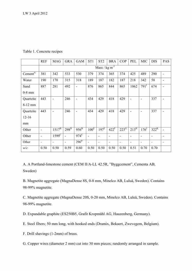
LW 3 April 2012

Table 1. Concrete recipes

REF MAG GRA GAM ST1 ST2 BRA COP PEL MIC DIS PAS

Mass / kg m-3

CementA 381 342 533 530 379 374 365 374 425 489 290 -

Water 190 170 315 318 189 187 182 187 218 342 58 -

Sand

0-8 mm

887 281 492 - 876 865 844 865 1062 791I 674 -

Quartzite

8-12 mm

443 - 246 - 434 429 418 429 - - 337 -

Quartzite

12-16

mm

443 - 246 - 434 429 418 429 - - 337 -

Other - 1517B 298D 956B 100E 197E 422F 223G 213H 176J 322K -

Other - 1599C - 974C - - - - - - - -

Other - - - 296D - - - - - - - -

w/c 0.50 0.50 0.59 0.60 0.50 0.50 0.50 0.50 0.51 0.70 0.70

A. A Portland-limestone cement (CEM II/A-LL 42.5R, ”Byggcement”, Cementa AB,

Sweden)

B. Magnetite aggregate (MagnaDense 8S, 0-8 mm, Minelco AB, Luluå, Sweden). Contains

98-99% magnetite.

C. Magnetite aggregate (MagnaDense 20S, 0-20 mm, Minelco AB, Luleå, Sweden). Contains

98-99% magnetite.

D. Expandable graphite (ES250B5, Grafit Kropmühl AG, Hauzenberg, Germany).

E. Steel fibers; 50 mm long, with hooked ends (Dramix, Bekaert, Zwevegem, Belgium).

F. Drill shavings (1-2mm) of brass.

G. Copper wires (diameter 2 mm) cut into 30 mm pieces; randomly arranged in sample.

LW 3 April 2012

H. Macroencapsulated paraffin based phase change material (Rubitherm PK, Rubitherm

Technologies GmbH, Berlin, Germany). Rice-shaped grains with a length of about 5 mm.

Melting temperature of 42 C.

I. Only the 0.5-8 mm fraction.

J. Microencapsulated paraffin based phase change material (Micronal PCM, BASF) with a

diameter of less than 0.5 mm. Melting temperature of 23 C.

K. Dispersion of paraffin based phase change compound (Micronal DS5007X, BASF) with

55% dry matter. Melting temperature of 26 C.

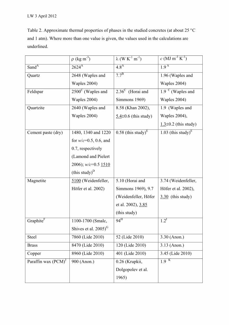
LW 3 April 2012

Table 2. Approximate thermal properties of phases in the studied concretes (at about 25 C

and 1 atm). Where more than one value is given, the values used in the calculations are

underlined.

(kg m-3) (W K-1 m-1) c (MJ m-3 K-1)

SandA 2624A 4.8A 1.9 A

Quartz 2648 (Waples and

Waples 2004)

7.7B 1.96 (Waples and

Waples 2004)

Feldspar 2500C (Waples and

Waples 2004)

2.36C (Horai and

Simmons 1969)

1.9 C (Waples and

Waples 2004)

Quartzite 2640 (Waples and

Waples 2004)

8.58 (Khan 2002),

5.40.6 (this study)

1.9 (Waples and

Waples 2004),

1.30.2 (this study)

Cement paste (dry) 1480, 1340 and 1220

for w/c=0.5, 0.6, and

0.7, respectively

(Lamond and Pielert

2006); w/c=0.5 1510

(this study)D

0.58 (this study)E 1.03 (this study)E

Magnetite 5100 (Weidenfeller,

Höfer et al. 2002)

5.10 (Horai and

Simmons 1969), 9.7

(Weidenfeller, Höfer

et al. 2002), 3.85

(this study)

3.74 (Weidenfeller,

Höfer et al. 2002),

3.30 (this study)

GraphiteF 1100-1700 (Smalc,

Shives et al. 2005)G

94H 1.2I

Steel 7860 (Lide 2010) 52 (Lide 2010) 3.30 (Anon.)

Brass 8470 (Lide 2010) 120 (Lide 2010) 3.13 (Anon.)

Copper 8960 (Lide 2010) 401 (Lide 2010) 3.45 (Lide 2010)

Paraffin wax (PCM)J 900 (Anon.) 0.26 (Krupkii,

Dolgopolev et al.

1965)

1.9 K

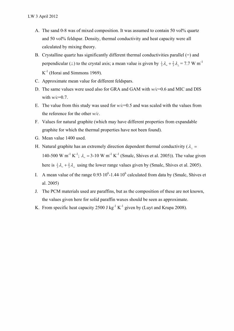
LW 3 April 2012

A. The sand 0-8 was of mixed composition. It was assumed to contain 50 vol% quartz

and 50 vol% feldspar. Density, thermal conductivity and heat capacity were all

calculated by mixing theory.

B. Crystalline quartz has significantly different thermal conductivities parallel (=) and

perpendicular () to the crystal axis; a mean value is given by 32

31 = 7.7 W m-1

K-1 (Horai and Simmons 1969).

C. Approximate mean value for different feldspars.

D. The same values were used also for GRA and GAM with w/c=0.6 and MIC and DIS

with w/c=0.7.

E. The value from this study was used for w/c=0.5 and was scaled with the values from

the reference for the other w/c.

F. Values for natural graphite (which may have different properties from expandable

graphite for which the thermal properties have not been found).

G. Mean value 1400 used.

H. Natural graphite has an extremely direction dependent thermal conductivity (

140-500 W m-1 K-1; 3-10 W m-1 K-1 (Smalc, Shives et al. 2005)). The value given

here is 32

31 using the lower range values given by (Smalc, Shives et al. 2005).

I. A mean value of the range 0.93106-1.44106 calculated from data by (Smalc, Shives et

al. 2005)

J. The PCM materials used are paraffins, but as the composition of these are not known,

the values given here for solid paraffin waxes should be seen as approximate.

K. From specific heat capacity 2500 J kg-1 K-1 given by (Luyt and Krupa 2008).

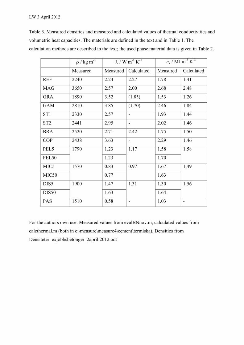
LW 3 April 2012

Table 3. Measured densities and measured and calculated values of thermal conductivities and

volumetric heat capacities. The materials are defined in the text and in Table 1. The

calculation methods are described in the text; the used phase material data is given in Table 2.

/ kg m-3 / W m-1 K-1 cv / MJ m-3 K-3

Measured Measured Calculated Measured Calculated

REF 2240 2.24 2.27 1.78 1.41

MAG 3650 2.57 2.00 2.68 2.48

GRA 1890 3.52 (1.85) 1.53 1.26

GAM 2810 3.85 (1.70) 2.46 1.84

ST1 2330 2.57 - 1.93 1.44

ST2 2441 2.95 - 2.02 1.46

BRA 2520 2.71 2.42 1.75 1.50

COP 2438 3.63 - 2.29 1.46

PEL5 1790 1.23 1.17 1.58 1.58

PEL50 1.23 1.70

MIC5 1570 0.83 0.97 1.67 1.49

MIC50 0.77 1.63

DIS5 1900 1.47 1.31 1.30 1.56

DIS50 1.63 1.64

PAS 1510 0.58 - 1.03 -

For the authors own use: Measured values from evalBNnov.m; calculated values from

calcthermal.m (both in c:\measure\measure4\cement\termiska). Densities from

Densiteter_exjobbsbetonger_2april.2012.odt

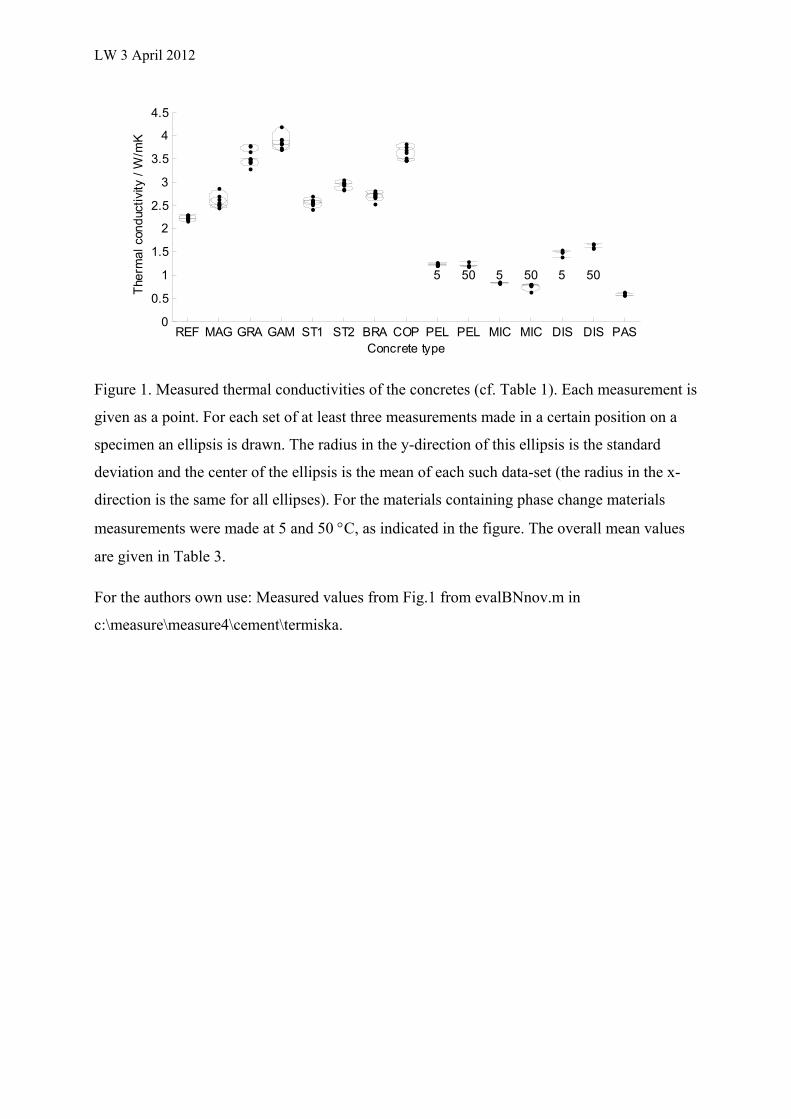
LW 3 April 2012

Figure 1. Measured thermal conductivities of the concretes (cf. Table 1). Each measurement is

given as a point. For each set of at least three measurements made in a certain position on a

specimen an ellipsis is drawn. The radius in the y-direction of this ellipsis is the standard

deviation and the center of the ellipsis is the mean of each such data-set (the radius in the x-

direction is the same for all ellipses). For the materials containing phase change materials

measurements were made at 5 and 50 C, as indicated in the figure. The overall mean values

are given in Table 3.

For the authors own use: Measured values from Fig.1 from evalBNnov.m in

c:\measure\measure4\cement\termiska.

REF MAG GRA GAM ST1 ST2 BRA COP PEL PEL MIC MIC DIS DIS PAS0

0.5

1

1.5

2

2.5

3

3.5

4

4.5

Concrete type

The

rma

l co

nd

ucti

vity

/ W

/mK

5 50 5 50 5 50

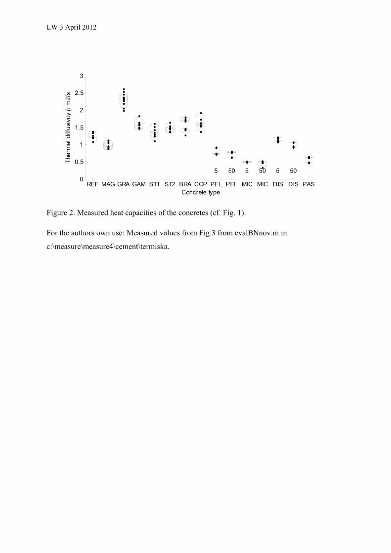
LW 3 April 2012

Figure 2. Measured heat capacities of the concretes (cf. Fig. 1).

For the authors own use: Measured values from Fig.3 from evalBNnov.m in

c:\measure\measure4\cement\termiska.

REF MAG GRA GAM ST1 ST2 BRA COP PEL PEL MIC MIC DIS DIS PAS0

0.5

1

1.5

2

2.5

3

Concrete type

The

rma

l d

iffu

sivi

ty /

m

2/s

5 50 5 50 5 50

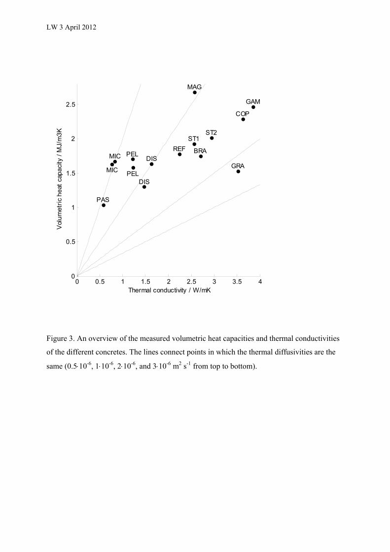
LW 3 April 2012

Figure 3. An overview of the measured volumetric heat capacities and thermal conductivities

of the different concretes. The lines connect points in which the thermal diffusivities are the

same (0.510-6, 110-6, 210-6, and 310-6 m2 s-1 from top to bottom).

0 0.5 1 1.5 2 2.5 3 3.5 40

0.5

1

1.5

2

2.5

REF

MAG

GRA

ST1ST2

BRA

COP

GAM

PELDIS

MIC PELDIS

MIC

PAS

Thermal conductivity / W/mK

Vol

um

etr

ic h

eat

cap

aci

ty /

MJ/

m3

K

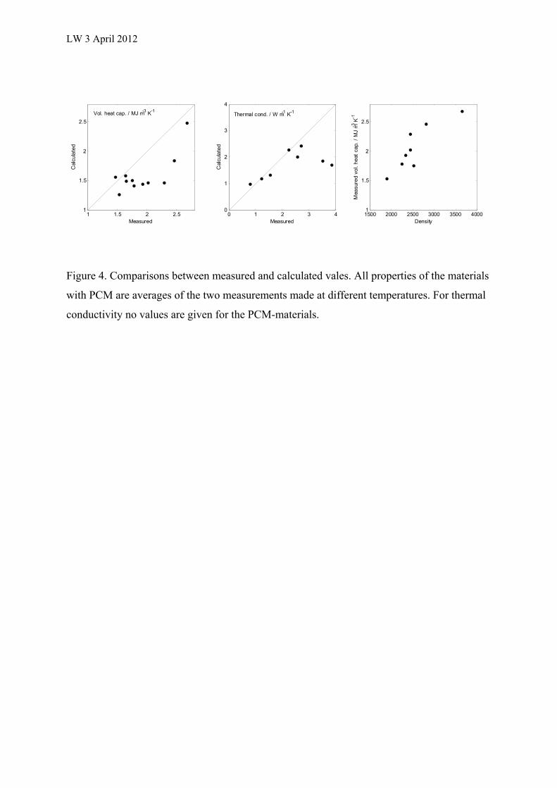
LW 3 April 2012

Figure 4. Comparisons between measured and calculated vales. All properties of the materials

with PCM are averages of the two measurements made at different temperatures. For thermal

conductivity no values are given for the PCM-materials.

1 1.5 2 2.51

1.5

2

2.5

Measured

Cal

cula

ted

Vol. heat cap. / MJ m-3 K-1

0 1 2 3 40

1

2

3

4

MeasuredC

alcu

late

d

Thermal cond. / W m-1 K-1

1500 2000 2500 3000 3500 40001

1.5

2

2.5

Density

Mea

sure

d v

ol.

hea

t ca

p. /

MJ

m-3 K

-1