Embed Size (px)
Citation preview
Elliptic & Parabolic Equations
Zhuoqun Wu, Jingxue Yin & Chunpeng Wang
Elliptic & Parabolic Equations

Elliptic & Parabolic Equations
Zhuoqun Wu, Jingxue Yin & Chunpeng Wang Jilin University, China
\JJS World Scientific NEW JERSEY • LONDON • S INGAPORE • BE IJ ING • S H A N G H A I • HONG KONG • TAIPEI • C H E N N A I
Published by
World Scientific Publishing Co. Pte. Ltd.
5 Toh Tuck Link, Singapore 596224
USA office: 27 Warren Street, Suite 401-402, Hackensack, NJ 07601
UK office: 57 Shelton Street, Covent Garden, London WC2H 9HE
British Library Cataloguing-in-Publication Data A catalogue record for this book is available from the British Library.
ELLIPTIC AND PARABOLIC EQUATIONS
Copyright © 2006 by World Scientific Publishing Co. Pte. Ltd.
All rights reserved. This book, or parts thereof, may not be reproduced in any form or by any means, electronic or mechanical, including photocopying, recording or any information storage and retrieval system now known or to be invented, without written permission from the Publisher.
For photocopying of material in this volume, please pay a copying fee through the Copyright Clearance Center, Inc., 222 Rosewood Drive, Danvers, MA 01923, USA. In this case permission to photocopy is not required from the publisher.
ISBN 981-270-025-0 ISBN 981-270-026-9 (pbk)
Printed in Singapore by B & JO Enterprise
Preface
Elliptic equations and parabolic equations are two important branches in the field of partial differential equations. These two kinds of equations arise frequently at the same time in many applications: elliptic equations arise from the stationary case and parabolic equations from the nonstationary case. In history, theories of them have been developed almost simultaneously. Many methods applied to elliptic equations are also available to parabolic equations, although some new methods are required to be developed for the latter. So far there have been numerous monographs focusing separately on each kind of equations, see [Ladyzenskaja and Ural'ceva (1968)], [Ladyzenskaja, Solonnikov and Ural'ceva (1968)], [Gilbarg and Trudinger (1977)], [Lieberman (1996)], [Chen and Wu (1997)], [Chen (2003)] and [Gu (1995)]. However, there are very few books treating them in combination. In this respect, the book [Oleinik and Radkevic (1973)] should be mentioned, in which the equations considered include not only both linear elliptic and parabolic equations, but also all kinds of linear degenerate elliptic equations of second order. However, in the framework of this book, parabolic equations are regarded as degenerate elliptic equations by treating the time variable and space variables equally and thus only the commonalities between these two kinds of equations are presented. As a matter of course, in such a book, it is impossible to discuss deeply the specific properties of each kind.
Prom our own experiences of teaching and research, we are aware of the necessity of writing a book which merges these two kinds of equations into an organic whole, involving the related basic theories and methods. This book is the result of a try following this idea, which is completed on the basis of lectures for graduate students majored in partial differential equations at Jilin University of China. The lectures have also been used at
VI Elliptic and Parabolic Equations
the summer school for graduate students in China. The purpose of this book is to provide an introduction to elliptic and
parabolic equations of second order for graduate students and young scholars who want to work in the field of partial differential equations. It is our hope that the book will be beneficial not only to stress the commonalities between these two kinds of equations, but also to expose the specific properties of each kind, so that the readers can efficiently learn the related knowledge by observing the relationship and contrasting the similarities and differences. An exhaustive theory of these two kinds of equations is outside the scope of this book. The book covers only the related basic theories and methods in a reasonable volume. More attention is paid to typical equations. In treating each kind of equations, usually we first give a detailed discussion on some typical equations and then discuss general equations in a brief fashion. Our principal intention is to prevent the complicate derivation due to the generality of equations in form from concealing and obscuring substantial of the argument. Emphasis is put on introducing methods and techniques rather than collecting theorems and facts.
The book consists of thirteen chapters. Some preliminary knowledge needed in the book is collected in Chapter
1, the main part of which is an introduction to the theory of Sobolev spaces and Holder spaces.
Linear equations are discussed in Chapter 2 through Chapter 9. Chapter 2 and Chapter 3 are devoted to weak solutions and the L2 theory of linear elliptic equations and parabolic equations respectively.
Properties of weak solutions are discussed in Chapter 4 and Chapter 5. In Chapter 4, we introduce two important methods, the De Giorgi iteration and the Moser iteration which are described only for some typical equations and applied only to the maximum estimates on weak solutions. Chapter 5 discusses Harnack's inequalities.
In Chapter 6 and Chapter 7, we establish Schauder's estimates for elliptic equations and parabolic equations respectively. Based on these estimates, we prove the existence of classical solutions in Chapter 8. In establishing Schauder's estimates, we apply Campanato's approach which is based on the important fact that the Holder continuity of functions can be described in an equivalent integral form. By means of this approach, the proof is relatively simple.
Chapter 9 is an argument of the Lp estimates which are used to discuss the existence of strong solutions.
The solvability of quasilinear equations is studied in Chapter 10 through
Preface vn
Chapter 12. Three methods are introduced, they are: the fixed point method (Chapter 10), the topology degree method (Chapter 11) and the monotone method (Chapter 12).
The book finishes with Chapter 13, which contains an investigation of elliptic and parabolic equations with degeneracy. The first part of this chapter deals with linear equations, namely, equations with nonnegative characteristic form. Quasilinear equations are discussed in the second part of this chapter.
As space is limited, we are not able to cover the study of fully nonlinear elliptic and parabolic equations in the book.
Wu Zhuoqun Yin Jingxue Wang Chunpeng
Jilin University, P. R. China August, 2006

Contents
Preface v
1. Preliminary Knowledge 1
1.1 Some Frequently Applied Inequalities and Basic Techniques 1 1.1.1 Some frequently applied inequalities 1 1.1.2 Spaces Ck(Q) and C#(0) 2 1.1.3 Smoothing operators 3 1.1.4 Cut-off functions 5 1.1.5 Partition of unity 6 1.1.6 Local flatting of the boundary 6
1.2 Holder Spaces 7 1.2.1 Spaces Ck'a(ty and Ck>a(n) 7 1.2.2 Interpolation inequalities 8 1.2.3 Spaces C2k+a>k+a/2(QT) 13
1.3 Isotropic Sobolev Spaces 14 1.3.1 Weak derivatives 14 1.3.2 Sobolev spaces Wk'p(Q) and W0
fe'p(ft) 15 1.3.3 Operation rules of weak derivatives 17 1.3.4 Interpolation inequality 17 1.3.5 Embedding theorem 19 1.3.6 Poincare's inequality 21
1.4 t-Anisotropic Sobolev Spaces 24
1.4.1 Spaces W£k<k(QT), W2pk>k(QT), Wf'k(QT), V2(QT)
and V(QT) 24 1.4.2 Embedding theorem 26 1.4.3 Poincare's inequality 28
ix
x Elliptic and Parabolic Equations
1.5 Trace of Functions in i/x(fi) 29 1.5.1 Some propositions on functions in H1(Q+) 29 1.5.2 Trace of functions in tf^fi) 33
1.5.3 Trace of functions in ^ ( Q r ) = W^21,1(Qr) 35
2. L2 Theory of Linear Elliptic Equations 39
2.1 Weak Solutions of Poisson's Equation 39 2.1.1 Definition of weak solutions 40 2.1.2 Riesz's representation theorem and its application . . 41 2.1.3 Transformation of the problem 43 2.1.4 Existence of minimizers of the corresponding
functional 44 2.2 Regularity of Weak Solutions of Poisson's Equation . . . . 47
2.2.1 Difference operators 47 2.2.2 Interior regularity 50 2.2.3 Regularity near the boundary 53 2.2.4 Global regularity 56 2.2.5 Study of regularity by means of smoothing operators 58
2.3 L2 Theory of General Elliptic Equations 60 2.3.1 Weak solutions 60 2.3.2 Riesz's representation theorem and its application . . 61 2.3.3 Variational method 62 2.3.4 Lax-Milgram's theorem and its application 64 2.3.5 Fredholm's alternative theorem and its application . 67
3. L2 Theory of Linear Parabolic Equations 71
3.1 Energy Method 71 3.1.1 Definition of weak solutions 72 3.1.2 A modified Lax-Milgram's theorem 73 3.1.3 Existence and uniqueness of the weak solution . . . . 75
3.2 Rothe's Method 79 3.3 Galerkin's Method 85 3.4 Regularity of Weak Solutions 89 3.5 L2 Theory of General Parabolic Equations 94
3.5.1 Energy method 94 3.5.2 Rothe's method 96 3.5.3 Galerkin's method 97
4. De Giorgi Iteration and Moser Iteration 105
Contents xi
4.1 Global Boundedness Estimates of Weak Solutions of Pois-son's Equation 105 4.1.1 Weak maximum principle for solutions of Laplace's
equation 105 4.1.2 Weak maximum principle for solutions of Poisson's
equation 107 4.2 Global Boundedness Estimates for Weak Solutions of the
Heat Equation I l l 4.2.1 Weak maximum principle for solutions of the homo
geneous heat equation I l l 4.2.2 Weak maximum principle for solutions of the nonho-
mogeneous heat equation 112 4.3 Local Boundedness Estimates for Weak Solutions of Pois
son's Equation 116 4.3.1 Weak subsolutions (supersolutions) 116 4.3.2 Local boundedness estimate for weak solutions of
Laplace's equation 118 4.3.3 Local boundedness estimate for solutions of Poisson's
equation 120 4.3.4 Estimate near the boundary for weak solutions of
Poisson's equation 122 4.4 Local Boundedness Estimates for Weak Solutions of the Heat
Equation 123 4.4.1 Weak subsolutions (supersolutions) 123 4.4.2 Local boundedness estimate for weak solutions of the
homogeneous heat equation 123 4.4.3 Local boundedness estimate for weak solutions of the
nonhomogeneous heat equation 126
5. Harnack's Inequalities 131
5.1 Harnack's Inequalities for Solutions of Laplace's Equation . 131 5.1.1 Mean value formula 131 5.1.2 Classical Harnack's inequality 133 5.1.3 Estimate of sup u 133
BBR
5.1.4 Estimate of inf u 135 BBR
5.1.5 Harnack's inequality 141 5.1.6 Holder's estimate 143
xii Elliptic and Parabolic Equations
5.2 Harnack's Inequalities for Solutions of the Homogeneous Heat Equation 145 5.2.1 Weak Harnack's inequality 146 5.2.2 Holder's estimate 155 5.2.3 Harnack's inequality 156
6. Schauder's Estimates for Linear Elliptic Equations 159
6.1 Campanato Spaces 159 6.2 Schauder's Estimates for Poisson's Equation 165
6.2.1 Estimates to be established 165 6.2.2 Caccioppoli's inequalities 168 6.2.3 Interior estimate for Laplace's equation 173 6.2.4 Near boundary estimate for Laplace's equation . . . 175 6.2.5 Iteration lemma 177 6.2.6 Interior estimate for Poisson's equation 178 6.2.7 Near boundary estimate for Poisson's equation . . . 181
6.3 Schauder's Estimates for General Linear Elliptic Equations 187 6.3.1 Simplification of the problem 188 6.3.2 Interior estimate 188 6.3.3 Near boundary estimate 191 6.3.4 Global estimate 193
7. Schauder's Estimates for Linear Parabolic Equations 197
7.1 t-Anisotropic Campanato Spaces 197 7.2 Schauder's Estimates for the Heat Equation 199
7.2.1 Estimates to be established 199 7.2.2 Interior estimate 200 7.2.3 Near bottom estimate 208 7.2.4 Near lateral estimate 214 7.2.5 Near lateral-bottom estimate 227 7.2.6 Schauder's estimates for general linear parabolic
equations 231
8. Existence of Classical Solutions for Linear Equations 233
8.1 Maximum Principle and Comparison Principle 233 8.1.1 The case of elliptic equations 233 8.1.2 The case of parabolic equations 236
Contents xiii
8.2 Existence and Uniqueness of Classical Solutions for Linear Elliptic Equations 240 8.2.1 Existence and uniqueness of the classical solution for
Poisson's equation 240 8.2.2 The method of continuity 246 8.2.3 Existence and uniqueness of classical solutions for
general linear elliptic equations 248 8.3 Existence and Uniqueness of Classical Solutions for Linear
Parabolic Equations 249 8.3.1 Existence and uniqueness of the classical solution for
the heat equation 250 8.3.2 Existence and uniqueness of classical solutions for
general linear parabolic equations 251
9. V Estimates for Linear Equations and Existence of Strong Solutions 255
9.1 LP Estimates for Linear Elliptic Equations and Existence and Uniqueness of Strong Solutions 255 9.1.1 LP estimates for Poisson's equation in cubes 255 9.1.2 LP estimates for general linear elliptic equations . . . 260 9.1.3 Existence and uniqueness of strong solutions for linear
elliptic equations 264 9.2 LP Estimates for Linear Parabolic Equations and Existence
and Uniqueness of Strong Solutions 266 9.2.1 LP estimates for the heat equation in cubes 266 9.2.2 LP estimates for general linear parabolic equations . 271 9.2.3 Existence and uniqueness of strong solutions for linear
parabolic equations 272
10. Fixed Point Method 277
10.1 Framework of Solving Quasilinear Equations via Fixed Point Method 277 10.1.1 Leray-Schauder's fixed point theorem 277 10.1.2 Solvability of quasilinear elliptic equations 277 10.1.3 Solvability of quasilinear parabolic equations 280 10.1.4 The procedures of the a priori estimates 282
10.2 Maximum Estimate 282 10.3 Interior Holder's Estimate 284
xiv Elliptic and Parabolic Equations
10.4 Boundary Holder's Estimate and Boundary Gradient Estimate for Solutions of Poisson's Equation 287
10.5 Boundary Holder's Estimate and Boundary Gradient Estimate 289
10.6 Global Gradient Estimate 296 10.7 Holder's Estimate for a Linear Equation 301
10.7.1 An iteration lemma 301 10.7.2 Morrey's theorem 302 10.7.3 Holder's estimate 303
10.8 Holder's Estimate for Gradients 307 10.8.1 Interior Holder's estimate for gradients of solutions . 307 10.8.2 Boundary Holder's estimate for gradients of solutions 308 10.8.3 Global Holder's estimate for gradients of solutions . 310
10.9 Solvability of More General Quasilinear Equations 310 10.9.1 Solvability of more general quasilinear elliptic
equations 310 10.9.2 Solvability of more general quasilinear parabolic
equations 311
11. Topological Degree Method 313
11.1 Topological Degree 313 11.1.1 Brouwer degree 313 11.1.2 Leray-Schauder degree 315
11.2 Existence of a Heat Equation with Strong Nonlinear Source 317
12. Monotone Method 323
12.1 Monotone Method for Parabolic Problems 323 12.1.1 Definition of supersolutions and subsolutions 324 12.1.2 Iteration and monotone property 324 12.1.3 Existence results 327 12.1.4 Application to more general parabolic equations . . . 330 12.1.5 Nonuniqueness of solutions 332
12.2 Monotone Method for Coupled Parabolic Systems 336 12.2.1 Quasimonotone reaction functions 337 12.2.2 Definition of supersolutions and subsolutions 337 12.2.3 Monotone sequences 339 12.2.4 Existence results 350 12.2.5 Extension 353
Contents xv
13. Degenerate Equations 355
13.1 Linear Equations 355 13.1.1 Formulation of the first boundary value problem . . 356 13.1.2 Solvability of the problem in a space similar to Hx . 361 13.1.3 Solvability of the problem in IP (ft) 362 13.1.4 Method of elliptic regularization 365 13.1.5 Uniqueness of weak solutions in Lp(ft) and regularity 366
13.2 A Class of Special Quasilinear Degenerate Parabolic Equations - Filtration Equations 368 13.2.1 Definition of weak solutions 369 13.2.2 Uniqueness of weak solutions for one dimensional
equations 371 13.2.3 Existence of weak solutions for one dimensional equa
tions 373 13.2.4 Uniqueness of weak solutions for higher dimensional
equations 378 13.2.5 Existence of weak solutions for higher dimensional
equations 381 13.3 General Quasilinear Degenerate Parabolic Equations . . . . 384
13.3.1 Uniqueness of weak solutions for weakly degenerate equations 385
13.3.2 Existence of weak solutions for weakly degenerate equations 393
13.3.3 A remark on quasilinear parabolic equations with strong degeneracy 399
Bibliography 403
Index 405
Chapter 1
Preliminary Knowledge
In this chapter, we provide some preliminary knowledge needed in this book. The central part is a brief introduction to the theory of Sobolev spaces and Holder spaces. Most results are stated without proof, but references containing detailed proofs are indicated. An exception is that, for the convenience of the reader, a thorough discussion about the trace on the boundary of functions in a class of special Sobolev spaces is presented. The reader is assumed to have some acquaintance with elementary knowledge of functional analysis. Some specific facts in this field will be quoted wherever we need in the following chapters.
1.1 Some Frequently Applied Inequalities and Basic Techniques
This section presents some frequently applied inequalities and basic techniques such as mollifying, cutting off, partition of unity and local flatting of the boundary.
1.1.1 Some frequently applied inequalities
Young's inequality Let a > 0, b > 0, p > 1, q > 1 and - + - = 1. P Q
Then
L a? b" ab< h —•
P Q It is called Cauchy's inequality when p = q = 2.
Replacing a, b by e1/pa, e - 1 / p 6 with e > 0 in the above inequality, we get
l
2 Elliptic and Parabolic Equations
Young's inequality with e Let a > 0, b > 0, e > 0, p > 1, q > 1 and
- + - = 1. Then P q
eaP £-l/PhQ ab< — + - < eap + e-q/pb".
p q
In particular, when p = q — 2, it becomes
ab < | a 2 + l 6 2 ,
which is called Cauchy's inequality with e.
The following inequalities for functions in Lp are used frequently:
Holder's inequality Let p > 1, q > 1 and - + - = 1. If f € LP(Q,),
g e Li(£l), then f • g e Ll(£l) and
/ \f(x)g(x)\dx < ||/(a:)||LP(n)||5(a;)||L,(n). Jn
In particular, when p = q = 2, it becomes
/ \f(x)g(x)\dx < \\f\\L'(n)\\9\\L'(n), Jo.
which is called Schwarz's inequality.
Minkowski's inequality Let 1 < p < +oo, f,g & Lp(0) . Then f + g G Lp(n) and
\\f + 9hv(n) < ll/l|Lp(n) + ll5l|Lp(n)-
Here and below, throughout this chapter, il is always assumed to be a domain of Mn, unless stated otherwise, although many propositions presented are valid when Si is merely an open set or even a measurable set.
1.1.2 Spaces Ck(fl) and C*(Sl)
Let k be a nonnegative number or oo.
Definition 1.1.1 Cfe(S"2) and Ck(Q) denote sets of all functions having continuous derivatives up to order fc on Si and Si respectively. Usually, we simply denote C°(Sl) and C°(Sl) by C(Sl) and C(Sl) respectively. Define
Preliminary Knowledge 3
the norm on Ck(0.) as follows
\a\<k Q
where a = (a i , • • • ,a n ) is called a multi-index, a\, • • • ,an are nonnegative integers, \a\ = a.\ H + an and
D<*u = dlalu
dx<? • • • dx%» '
It is easy to verify that endowed with the norm defined above, Ck(Q) is a Banach space (see [Chen and Wu (1997)], [Adams (1975)]).
Definition 1.1.2 For a function u(x) on fi, we define
suppu = { i € (1; u{x) ^ 0}
and call it the support of u(x).
Definition 1.1.3 CQ (Cl) denotes the set of all functions in Cfe(f2) whose supports are compact in 0 . Usually we simply denote CQ(Q) by Co(fi).
1.1.3 Smoothing operators
Approximating a given function by smooth functions is a basic technique used frequently in the study of partial differential equations. There have been a variety of ways to this purpose, among them is the following method of mollification.
Let j(x) € Co°(Rn) be a nonnegative function, vanishing outside the
unit ball Bi(0) = {x € Rn;\x\ < 1} and satisfying / j(x)dx = 1. A
typical example is
j(x) =\A {O, \x\>l,
where
A = [ eiAN'-D^. -/Si(O)
Obviously for any e > 0, the function
j'W = hj (f) -
4 Elliptic and Parabolic Equations
vanishes outside the ball Be(0) = {x € Rn; \x\ < e} and / jE(x)dx = 1.
Definition 1.1.4 For a function u £ Ljoc(Rn), the operator J£ defined by
Jeu{x) = (je • u)(a:) = / je(x - y)u(y)dy
is called a smoothing operator, Jsu(x) the mollification of u, and je(x) the mollifier or kernel of radius e of the operator J£.
Here and below, for any open set Q, c E", we denote by Lloc(Q) the set of all locally integrable functions in fi.
Proposition 1.1.1 Let u be a function defined on M.n, vanishing outside a bounded domain Cl.
i) Ifue Z , 1 ^ ) , then J£u <E C°°(Rn). ii) 7/suppu C 0 and dist(suppu, dd) > e, then Jeu G CQ°(Q).
Hi) Ifue Lp(Q,)(l <p< +oo), then JEu € LP(Q) and
\\Jeu\\Lp(n) < ||u||LP(n), lim | | J e u - u | | i P ( n ) = 0.
iv) Ifue C(n), G c G c i l , t/ien
uniformly on G. v)Ifue C(U), then
lim J£u(x) = u(x)
lim JEu{x) = u(x) e—>0+
uniformly on Q.
Corollary 1.1.1 C^°(fi) is dense in Lp(fi)(p > 1).
For the proof of Proposition 1.1.1 and Corollary 1.1.1, we refer to [Adams (1975)] Chapter 2.
From the definition of smoothing operators, we see that the value of the mollification of a function at a point depends on the value of the function in the e-neighborhood of this point. So in approximating a given function at the points near the boundary, the method of mollification stated above is not available. In this case,we may mollify the function after supplementing its definition, say, letting it equal zero outside Cl, and use some modified mollifiers. As an example, we consider the mollification of a function near
Preliminary Knowledge 5
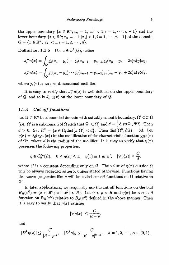
the upper boundary {x G Rn;xn = 1, \xi\ < l , i = 1, • • • ,n — 1} and the lower boundary {x e R"; xn = — 1, \xi\ < 1, i = 1, • • • , n — 1} of the domain Q = {x S R"; \xi\ < 1, i = 1,2, • • • , n}.
Definition 1.1.5 For u e L1(Q), define
J£~u(x) = / je(xx - y{) • • -jeixn-i - 2/„_i)je(x„ - yn - 2e)u(y)dy, JQ
J+u(x) = / je(xi - yx) • • • je{xn-i - yn-i)je(xn - Vn + 1e)u(y)dy, JQ
where j £ ( r ) is an one dimensional mollifier.
It is easy to verify that J~u(x) is well defined on the upper boundary of Q, and so is J+u(x) on the lower boundary of Q.
1.1.4 Cut-off functions
Let O C R" be a bounded domain with suitably smooth boundary, sT CC £1
(i.e. fi' is a subdomain of il such that Q C Cl) and d = -dist(fi ' , 9fi). Then d > 0. Set Q," = {x <= Si; dist(:r, iY) < d}. Then dist(Q",9sl) = 3d. Let ry(x) = Jd(xn" (%)) be the mollification of the characteristic function xn" (x)
of fi", where d is the radius of the mollifier. It is easy to verify that rj(x)
possesses the following properties:
^GCo^Sl) , 0 < 7 7 ( x ) < l , v(x) = lmSl', |V77(x) |<^ ,
where C is a constant depending only on si. The value of j](x) outside si will be always regarded as zero, unless stated otherwise. Functions having the above properties like rj will be called cut-off functions on si relative to Si'.
In later applications, we frequently use the cut-off functions on the ball BR(X°) = {x e Rn; \x - x°\ < R}. Let 0 < p < R and rj(x) be a cut-off function on BR(X°) relative to Bp(x°) defined in the above manner. Then it is easy to verify that rj(x) satisfies
| V ^ ) | < ^ ,
and
I ^ V * ) ! <T7T^k> lDhV}a< , D °,k+a, fc = l , 2 , - . . , a € ( 0 , l ) , \R-p\k' l ma-\R-p\
6 Elliptic and Parabolic Equations
where C is a universal constant independent of R, p, k and a. For the definition of {Dkrj\a, see §1.2.
In studying the properties such as regularity of solutions, we always confine ourselves to the consideration in a small neighborhood for the moment. An important measure to localize the problem is the usage of the cut-off functions. In this way, all local properties of the given function are retained and no influence outside the small neighborhood has to be considered.
1.1.5 Partition of unity
As observed above, we can localize the problem by using cut-off functions. In the study of partial differential equations, we also need frequently to integrate the result obtained by localization to deduce a global one. To this end, we need another measure, called, partition of unity. The following is a basic theorem on the partition of unity, for the proof, we refer to [Adams (1975)] Chapter 2 or [Cui, Jin and Lu (1991)] Chapter 1.
Theo rem 1.1.1 Let K C K" be a compact subset, U\,--- ,UN be an open covering of K. Then there exist functions rji £ CQ°(UI),- • • ,TJN € Co°{UN), such that
i)0< ru(x) < 1, VxeUi (i = 1, • • • , N); N
a) ^2TH(X) = i, VxeK.
i = l
We call 771, • • • ,T]N a partition of unity associated to U\, • • • , UN-
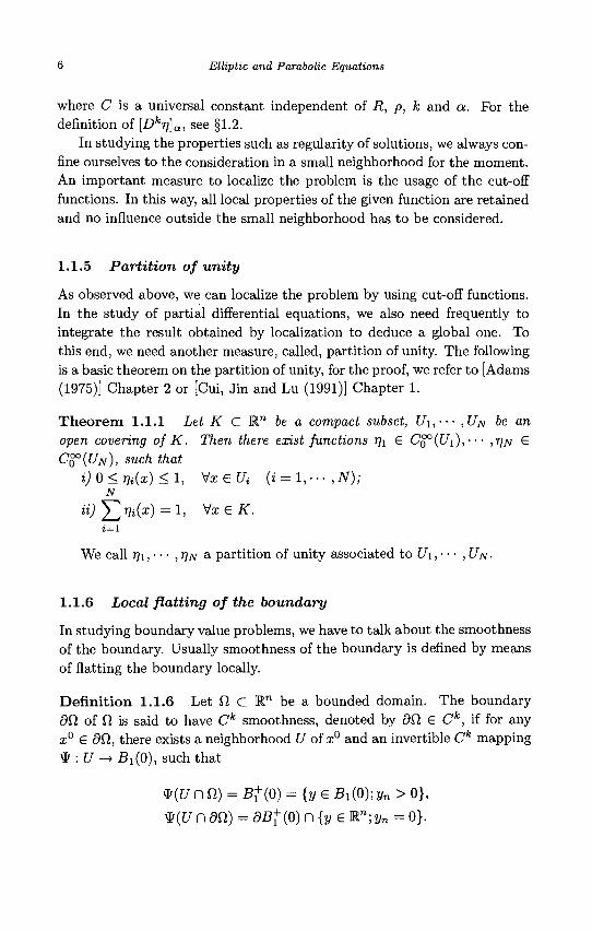
1.1.6 Local flatting of the boundary
In studying boundary value problems, we have to talk about the smoothness of the boundary. Usually smoothness of the boundary is denned by means of flatting the boundary locally.
Definition 1.1.6 Let fl C E n be a bounded domain. The boundary dQ. of Q, is said to have Ck smoothness, denoted by 9 0 € Ck, if for any x° e dil, there exists a neighborhood U of x° and an invertible Ck mapping * : U -* Bi(0), such that
tf(17nfl) = B+(0) - {y G Bi(0);y„ > 0},
* ( [ / n dSl) = dB+{0) n{ye Rn; yn = 0}.
Preliminary Knowledge 7
As we will see later, to discuss the properties of a function near the boundary, we usually flat the boundary locally in this way to transform the original problem locally into a problem on a domain with a superplane as its lower boundary.
1.2 Holder Spaces
1.2.1 Spaces Ck'a(H) and Ck'a(il)
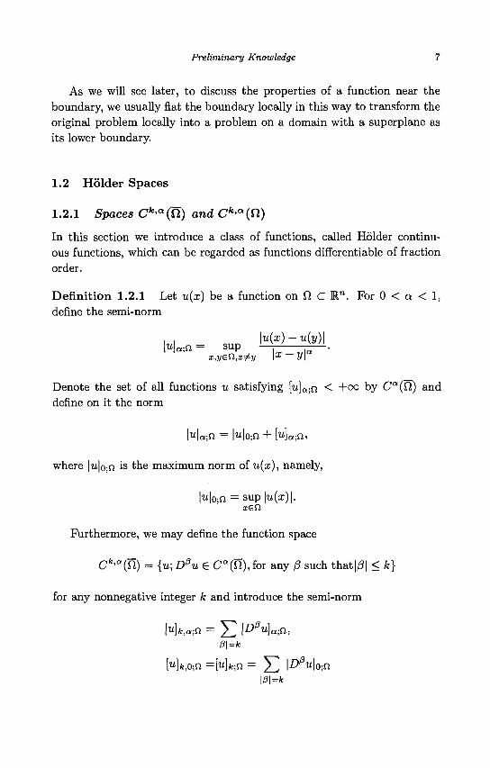
In this section we introduce a class of functions, called Holder continuous functions, which can be regarded as functions differentiable of fraction order.
Definition 1.2.1 Let u(x) be a function on O C R". For 0 < a < 1, define the semi-norm
[u\a.Q = sup —| | a—•
Denote the set of all functions u satisfying [u]a-Q < +oo by Ca(Q) and define on it the norm
Ma; f i = Mo-n + [u}a;Q,
where |u|o;n is the maximum norm of u(x), namely,
|u|o;n = sup|u(a;)|. xefi
Furthermore, we may define the function space
Ck'a(Ti) = {u\D0u G Ca(fi),for any (3 such that|/?| < k}
for any nonnegative integer k and introduce the semi-norm
\P\=k
Mfc,o;n =[u]k-n = 5 2 \D0u\o-,a |/3|=fc-
8 Elliptic and Parabolic Equations
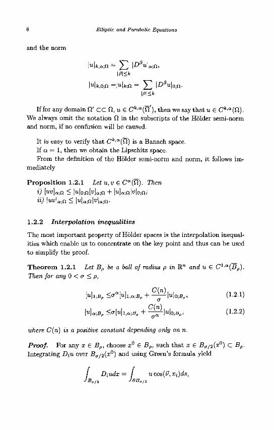
and the norm
\u\k,a;U = ^ Z \D0u\<*;fl, \0\<k
l«|fc,o;n =\u\k-,n = Y2 l - ^ ^ k n -l/3|<fc
If for any domain SI' CC Si, u € Cfc 'a(fi'), then we say that u e Ck<a(Sl). We always omit the notation SI in the subscripts of the Holder semi-norm and norm, if no confusion will be caused.
It is easy to verify that Ck'a(Sl) is a Banach space. If a = 1, then we obtain the Lipschitz space. Prom the definition of the Holder semi-norm and norm, it follows im
mediately
Proposition 1.2.1 Let u,v £ C a ( 0 ) . Then i) [uv]a-n < |u|0;nMa ;n + Ma ;n|«|o ;n; ii) \uv\a;n < \u\a.tn\v\a-n.
1.2.2 Interpolation inequalities
The most important property of Holder spaces is the interpolation inequalities which enable us to concentrate on the key point and thus can be used to simplify the proof.
Theorem 1.2.1 Let Bp be a ball of radius p in R™ and u e C 1 , a (B p ) . Then for any 0 < a < p,
Mi i B p <aa[u]ha]Bp + £ M | „ | 0 ; B (1.2.1)
[u}a;Bp <<TMl,«iB, + ^ l « | o ; f l p , (1-2.2)
where C(n) is a positive constant depending only on n.
Proof. For any x £ Bp, choose x° G Bp, such that x € Ba/2(x°) C Bp. Integrating Dtu over B(T/2(x°) and using Green's formula yield
/ Diudx = / ucos(v,Xi)ds, JB0/2 J9Ba/2
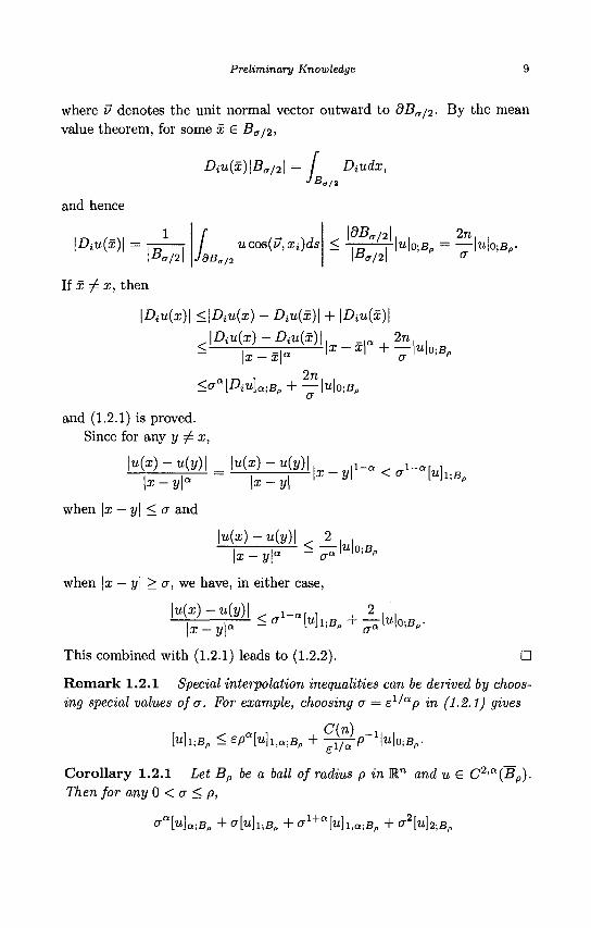
Preliminary Knowledge 9
where V denotes the unit normal vector outward to dBa/2- By the mean value theorem, for some x £ Ba/2,
Diu(x)\B, a/21 = / A udx,
and hence
\Diu(x)\
If x ^ x, then
B v/2\ / ucos(u,Xi)ds
JdBa/2
^ \dBaf2\ 2n. .
><T/2| O \B„
\Diu(x)\ <\Diu{x) - Diu(x)\ + \Diu(x)\
< \Dtu(x) - Diu(x)\
\x — xv
2n X-X\a + |u|o;Bp
2n, <0-a[DiU)a-Bp -\ |u|o;B,
and (1.2.1) is proved. Since for any y =fi x,
\x-y\a
when \x — y\ < a and
u{x) - u(y)\ _ \u(x) - u(y)\ ^ _ ^_a < ai-a[u]
\x-y\
u(x)-u(y)\ 2 < — I«IO ;BP \x — y\a a
when \x — y\ > a, we have, in either case
\u(x)-u(y)\ _ , | | a < ^ - a N l ; B p + - H 0 ; B p .
\x-y
This combined with (1.2.1) leads to (1.2.2). D
Remark 1.2.1 Special interpolation inequalities can be derived by choosing special values of a. For example, choosing a = £xlap in (1.2.1) gives
r i ^ „ , , C(n) _ i , . Ml|Bp < eP Ml,a;Bp + —yf^P MO;Bp-
Corollary 1.2.1 Let Bp be a ball of radius p in Rn and u € C2'a(Bp). Then for any 0 < a < p,
CrQMa;Bp +^Ml ;B p +0-1+a[w]1 ,a ;Bp +0-2H2 ;Bp
10 Elliptic and Parabolic Equations
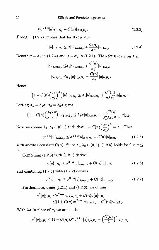
<a2+a[u}2,a;Bp + C{n)\u\Q,Bp. (1.2.3)
Proof. (1.2.2) implies tha t for 0 < a < p,
Ml,a ;B , < Cr{u}2,a;Bp + - ^ M l ; B p - (1-2-4)
Denote a = CTI in (1.2.4) and CT = CT2 in (1.2.1). Then for 0 < <7I,CT2 < p,
r i ^ r l C ( n ) r i
Ml,a;B„ <0-lM2,a;Bp + — ^ M l ; B p , °1
Ml;Bp <^2 Ml,a;Bp + Mo;Bp-&2
Hence
( l - C ( n ) ( ^ ) )[u]l,a;Bp < ^ l [ « ] a , a j B p + - ^ 5 ^ - H o ; B p .
Letting o-! = AICT, CT2 = A2CT gives
( l - C ( n ) ( ^ ) ) M l , a ; B p < AlCT[u]2,a;Bp + A a A J l + 1 M o ; B , -
/ A 2 \ a
Now we choose A:, A2 € (0,1) such that 1 - C(ra) (--^ 1 = Ax. Then
CT1+>]l,a;B„ < CT2+>]2,a;Bp + C ( n ) M o ; B p (1-2.5)
with another constant C(n). Since Ai, A2 £ (0,1), (1.2.5) holds for 0 < a <
P-Combining (1.2.5) with (1.2.1) derives
<r[«]i;B, < °2+a[uh,a;Bp + C(n)\u\0-Bp (1-2.6)
and combining (1.2.5) with (1.2.2) derives
Ga{u]a;Bp < a 2 + > ] 2 , a ; B p + C ( n ) | u | o ; B p . (1-2-7)
Furthermore, using (1.2.1) and (1.2.6), we obtain
<r2[uh;BP <cT2+a[u}2,a;Bp+C(n)a[u}1.,Bp
<(1 + C(n))a2+a[u}2,a;Bp + C\n)\u\0,Bp.
With ACT in place of cr, we are led to
<J2[u)2,Bp < (1 + C(n))A<V2+>]2,a;Bp + ( ^ ) V|O ;BP
Preliminary Knowledge 11
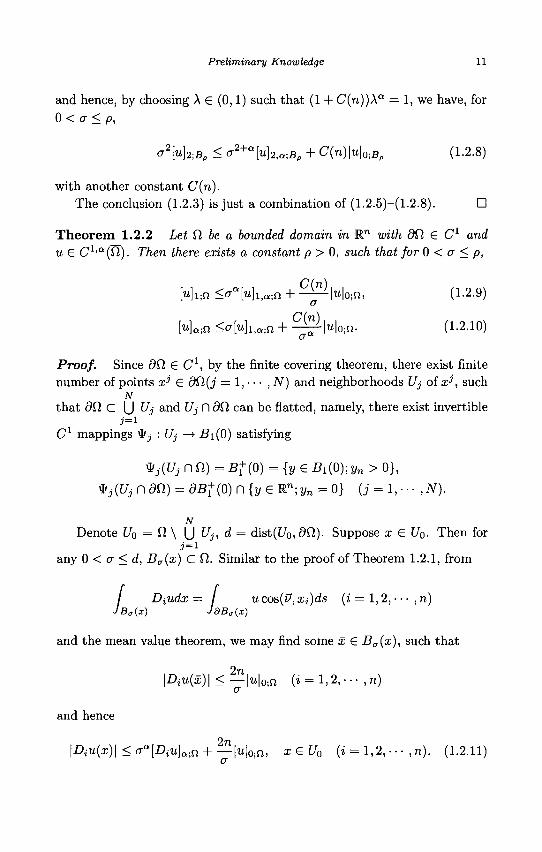
and hence, by choosing A G (0,1) such that (1 + C(n))Xa = 1, we have, for 0 < a < p,
v2[uh;Bp < o-2+a[u]2^Bf, + C(n)\u\0-Bp (1-2.8)
with another constant C(n). The conclusion (1.2.3) is just a combination of (1.2.5)-(1.2.8). •
Theo rem 1.2.2 Let £1 be a bounded domain in Rn with 9 0 G C1 and u G C 1 , a (0 ) . Then there exists a constant p > 0, such that for 0 < a < p,
Mi ;n <<r>] i , Q ; n + ^ M o ; n , (1-2.9) a
[u]a;n <ffHi,a ;n + - T r M o j n - (1.2.10)
Proof. Since 9 0 G C1 , by the finite covering theorem, there exist finite number of points x* G dQ(j = 1, • • • ,N) and neighborhoods Uj of x\ such
N
that 9 0 C |J Uj and Uj n 90 can be flatted, namely, there exist invertible
C 1 mappings ^ j : Uj —> B\ (0) satisfying
t i ^ n f i ) = B+(0) = {y G JBi(0);»n > 0},
* j ([/,• n 90) = 9B+ (0) n {y G Rn; y„ = 0} (j = 1, • • • , N).
N Denote U0 = O \ |J Uj, d = dist((70,9O). Suppose x G UQ. Then for
j = i any 0 < a < d, Ba(x) c O. Similar to the proof of Theorem 1.2.1, from
/ Diudx — I ucos(u,Xi)d. JBa(x) JdB„{x)
s (i = 1,2,-•• ,n)
and the mean value theorem, we may find some x G Ba(x), such that
2n \Diu{x)\<—|u|0;n (i = 1,2, ••• ,n)
<r
and hence
2n |A«(a:)| < f f l A i ; ! i + - | « | o ; n , a; G C/0 (» = 1,2, • • • ,n). (1.2.11)
12 Elliptic and Parabolic Equations
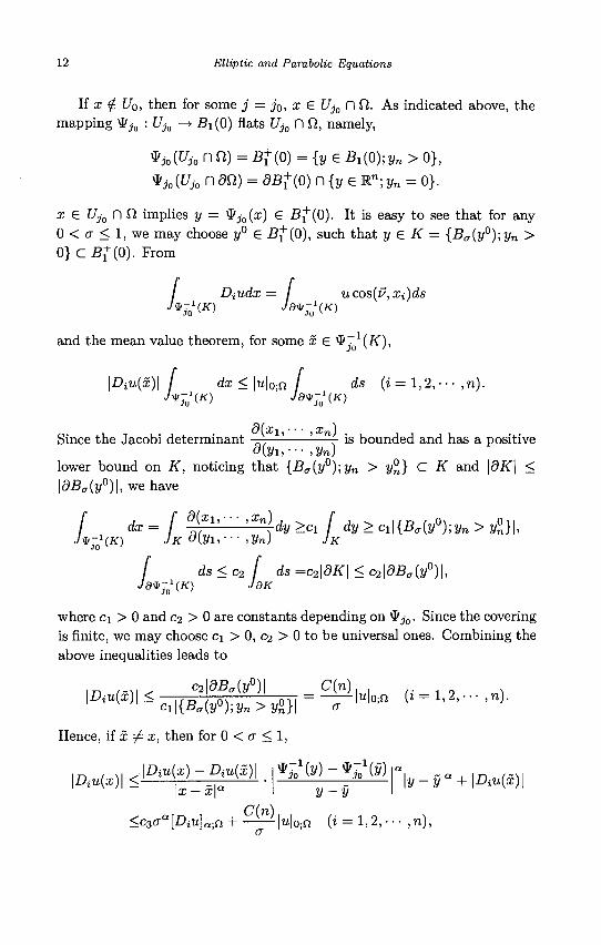
If x £ Uo, then for some j = j 0 , x G Ujo n fi. As indicated above, the mapping tyj0 : Ujo —> .Bi(O) flats f/,0 ("1 fi, namely,
*jo(Ujo n fi) = J 5 + ( 0 ) = {y G J5i(0);y„ > 0},
*io(uio n an) = dB+(o) n {y G R" ; yn = o}.
a; G Uj0 n fi implies j / = ^j0(x) G .Bj*"(0). It is easy to see that for any 0 < a < 1, we may choose y° G B^(0), such that y G K = {Ba(y°);yn > 0} C Bf(0). Prom
/ Diudx = u cos(i?, Xi)ds
and the mean value theorem, for some x G ^~^{K),
\Diu(x)\ I dx<\u\0-n ds (i = 1,2,• • • , n).
d(x\ • • • x ) Since the Jacobi determinant —.—- — r- is bounded and has a positive
o(yi,--- ,yn) lower bound on K, noticing that {B(7(y°);yn > y°} C K and \dK\ < \dBtT(y°)\, we have
f dx= [ f%Zli—>^dy >Cl [ dy> Cl\{Ba(y°);yn > y°n}\, J*-*(.!<) JK o(yu--- ,yn) JK
f ds<c2 [ ds =c2\0K\ < c2\dBa{y°)\, JdVjJ (K) JdK
where C\ > 0 and c2 > 0 are constants depending on ^jQ. Since the covering is finite, we may choose c\ > 0, c2 > 0 to be universal ones. Combining the above inequalities leads to
m c2\dBa(y°)\ C(n). | A u ( 3 ; ) l ^ e 1 | { g g ( W ° ) ; I f a > g o } | = — 1 " ^ (• = ^ • • • ,„).
Hence, if x ^ x, then for 0 < a < 1,
|Aw(a;)| < J —•—. • - ^ z^ \y - y\a + \Diu(x)\ \x — x\ y-y
<c3aa{Diu]a.Q + |u|o;n (i = l ,2, ••• ,n),
Preliminary Knowledge 13
where C3 > 0 is a constant independent of a and jo, y — *(x) and y = ^{x). This implies that for 0 < a < c3 'a ,
| A " ( x ) | < a a [ A u ] a ; f i + — M 0 ; f i , ^ ^ U0 (» = 1, 2, • • - , Tl) (1 .2 .12)
with another constant C(n). Let p = min {d,c\/a}. Then (1.2.9) follows from (1.2.11), (1.2.12). We
may argue as Theorem 1.2.1 to further prove (1.2.10). •
Corollary 1.2.2 Let Q be a bounded domain in R™ with dQ G C1 and u G C2'a(Q). Then there exists a constant p > 0, such that for 0 < a < p,
ffaMa;n + o-[u]Ua + o-1+a[u]1,Q;n + o-2[u\2-a
< < T 2 + > ] 2 , a ; f i + C ( r i ) M o ; n .
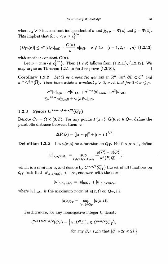
1.2.3 Spaces C2k+a'k+a/2(QT)
Denote QT = fi X (0,T). For any points P(x,t), Q(y,s) G QT, define the parabolic distance between them as
d(P,Q) = (\x-y\2 + \t-s\)1/2.
Definition 1.2.2 Let u(x, t) be a function on QT- For 0 < a < 1, define
, , \u(P)-u(Q)\ M a , a / 2 ; Q T = SUP ,
P,QeQT,P^Q da{P,Q)
which is a semi-norm, and denote by Ca'a/2(QT) the set of all functions on QT such that [u]a>a/2-QT < +oo, endowed with the norm
\u\a,a/2;QT = \UW,QT + [ U ]a ,a /2 ;Q T ,
where |u|o,QT ' s the maximum norm of u(x, t) on QT, i.e.
\U\O-QT = sup |u(a;,t)|. (x,t)GQr
Furthermore, for any nonnegative integer k, denote
C2k+a'h+a/2(QT) = \u-DPDrtu G Ca'a/2(QT),
for any f3,r such that |/3| + 2r < 2fc|,
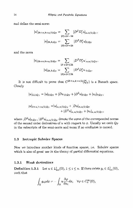
14 Elliptic and Parabolic Equations
and define the semi-norm
M 2 fc+a ,k+a /2 ;Q T = 2 j i ^ Dtu]a,a/2;QT> \0\+2r=2k
[u]2k,k;QT = J2 \DPDrtu\0-QT
|/3|+2r=2fc
and the norm
\u\2k+a,k+a/2;QT = 2^, \D Dtu\a,a/2;QT> \0\+2r<2k
\u\2k,k;QT = ^ 2 \DPD>\0;QT-|/3|+2r<2fc
It is not difficult to prove that C2k+a'k+a/2(QT) is a Banach space. Clearly
|«|2,1;QT = \UW,QT + \DUW,QT + \D2U\0;QT + \ut\o-,QT,
\u\2+a,l+a/2;QT — \u\a,a/2;QT + \^u\a,a/2;QT
+ \D u\a,a/2;QT + \ut\a,a/2;QT,
where | D 2 U | 0 ; Q T , |-D2u|a,a/2;QT denote the sums of the corresponded norms of the second order derivatives of u with respect to x. Usually we omit QT in the subscripts of the semi-norm and norm if no confusion is caused.
1.3 Isotropic Sobolev Spaces
Now we introduce another kinds of function spaces, i.e. Sobolev spaces which is also of great use in the theory of partial differential equations.
1.3.1 Weak derivatives
Definition 1.3.1 Let u £ L]oc(Sl), l<i<n. If there exists gt G Lloc(Cl), such that
/ gupdx = - f u^dx, V<p G C0°°(fi), Ja JQ clxi
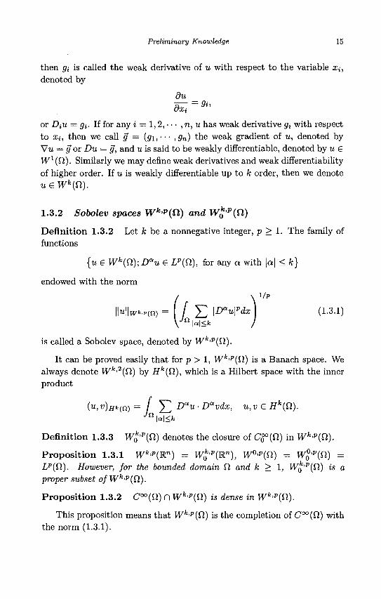
Preliminary Knowledge 15
then (ft is called the weak derivative of u with respect to the variable a^, denoted by
du a - =9i' axi
or DiU = gi. If for any i = 1,2, • • • , n, u has weak derivative <7J with respect to Xi, then we call g = (gi, • • • ,gn) the weak gradient of u, denoted by Vu = g or £>u = p, and u is said to be weakly differentiate, denoted by u £ W1(fi). Similarly we may define weak derivatives and weak differentiability of higher order. If u is weakly differentiate up to k order, then we denote u £ Wk(tl).
1.3.2 Sobolev spaces Wfe'P(ft) and W0fe,p(ft)
Definition 1.3.2 Let k be a nonnegative integer, p > 1. The family of functions
{u £ Wk(n); Dau £ LP{Q), for any a with \a\ < k]
endowed with the norm
IMIiv*.-(n)= ( / £ \Dau\pdx\ (1-3.1)
VnH<* / is called a Sobolev space, denoted by Wk'p(Cl).
It can be proved easily that for p > 1, Wk'p(Q) is a Banach space. We always denote Wk'2(Q.) by Hk(Q), which is a Hilbert space with the inner product
(«.v)ff*(n) = / H Dau-Davdx, u,v £ Hk(Sl).
Definition 1.3.3 W%,p(ft) denotes the closure of Cg°(fi) in Wk'p(£l).
Proposition 1.3.1 Wk>p(Rn) = W0fc'p(Rn), W°'p{Sl) = W°'p(^) =
Lp(fi). However, for the bounded domain 0, and k > 1, W0'P(Q) is a
proper subset ofWk'p(Q).
Proposition 1.3.2 C°°(ft) D Wk'p{n) is dense in Wk>p{Q).
This proposition means that Wk'p{n) is the completion of C°°(ft) with the norm (1.3.1).
16 Elliptic and Parabolic Equations
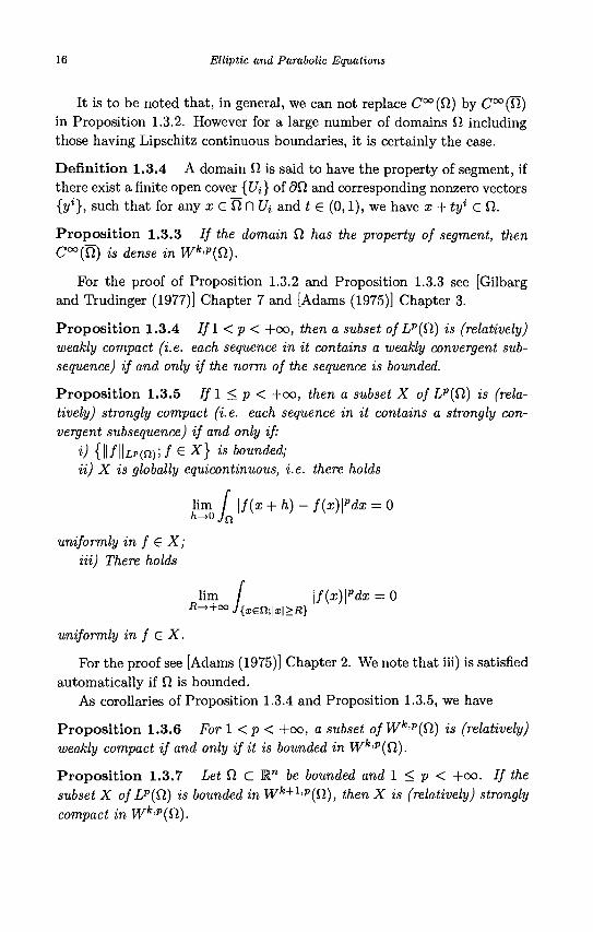
It is to be noted that, in general, we can not replace C°°(fi) by C°°(Q) in Proposition 1.3.2. However for a large number of domains Q. including those having Lipschitz continuous boundaries, it is certainly the case.
Definition 1.3.4 A domain Cl is said to have the property of segment, if there exist a finite open cover {C/j} of dd and corresponding nonzero vectors {y1}, such that for any x G Q, f~l U% and t G (0,1), we have x + tyi e $1
Proposition 1.3.3 / / the domain CI has the property of segment, then C°°(fi) is dense in Wk'p{Q).
For the proof of Proposition 1.3.2 and Proposition 1.3.3 see [Gilbarg and Trudinger (1977)] Chapter 7 and [Adams (1975)] Chapter 3.
Proposition 1.3.4 Ifl<p< +oo, then a subset of LP(Q) is (relatively) weakly compact (i.e. each sequence in it contains a weakly convergent subsequence) if and only if the norm of the sequence is bounded.
Proposition 1.3.5 If 1 < p < +oo, then a subset X of LP(Q) is (relatively) strongly compact (i.e. each sequence in it contains a strongly convergent subsequence) if and only if:
i) {||/||Lp(n);/ G X} is bounded; ii) X is globally equicontinuous, i.e. there holds
lim / \f{x + h)-f(x)\pdx = 0
uniformly in f € X; Hi) There holds
lim / \f(x)\pdx = 0
uniformly in f S X.
For the proof see [Adams (1975)] Chapter 2. We note that iii) is satisfied automatically if Cl is bounded.
As corollaries of Proposition 1.3.4 and Proposition 1.3.5, we have
Proposition 1.3.6 For 1 < p < +oo, a subset ofWk'p(Q) is (relatively) weakly compact if and only if it is bounded in Wk'p(Q).
Proposition 1.3.7 Let Q, C Rn be bounded and 1 < p < +oo. / / the subset X of Lp(£l) is bounded in Wk+1'P(Q), then X is (relatively) strongly compact in Wk,p(Q).
Preliminary Knowledge 17
Here we merely present a sufficient condition for a subset of Wk+1'P(Q) to be (relatively) strongly compact in the case of bounded domain fi, which is enough for our later usage.
1.3.3 Operation rules of weak derivatives
Some operation rules in calculus can be extended to weak derivatives by the approximation theorem(Proposition 1.1.1).
Proposi t ion 1.3.8 Let u, v G H^f i ) . Then
d(uv) dv du OXi OXi OXi
Proposition 1.3.9 Let Q,D be domains ofRn, u(x) G W1^) and $ = ($i , • • • , $„) : D —> f2 be a continuously differential mapping. Then
du($(y)) _ ^ d$j du k = 1 n
dVk JT[ dVk dXi'
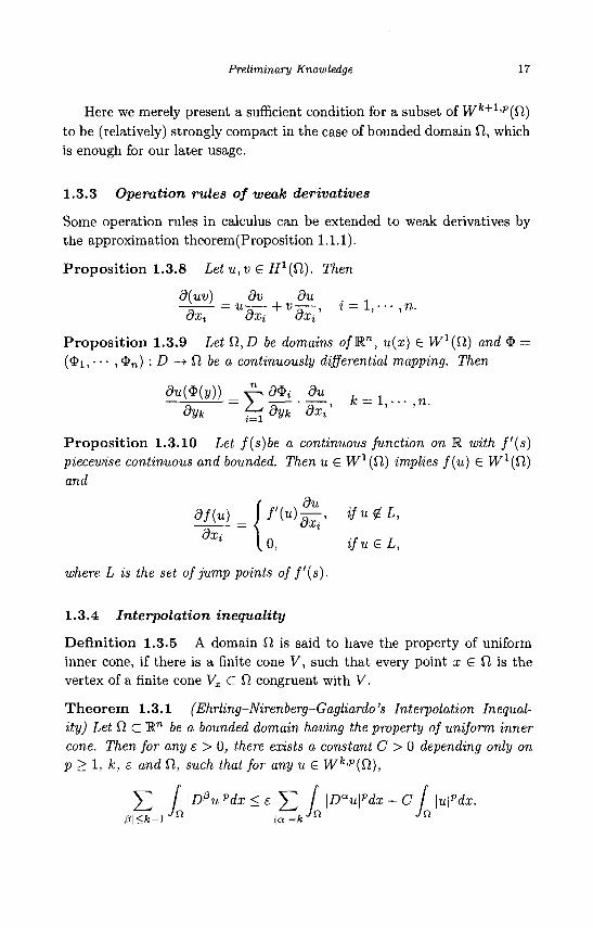
Proposition 1.3.10 Let f(s)be a continuous function on M with f'(s) piecewise continuous and bounded. Then u G W1(fi) implies f(u) £ W1(fi) and
a/(«) = f/'(w)^> «/w^L-dXi \ o , t /uGL,
uViere L is £/ie se£ of jump points of f'(s).
1.3.4 Interpolation inequality
Definition 1.3.5 A domain Q is said to have the property of uniform inner cone, if there is a finite cone V, such that every point x G ft is the vertex of a finite cone Vx C ft congruent with V.
Theorem 1.3.1 (Ehrling-Nirenberg-Gagliardo's Interpolation Inequality) Let ft C Mn be a bounded domain having the property of uniform inner cone. Then for any e > 0, there exists a constant C > 0 depending only on p > 1, k, £ and ft, such that for any u G Wk,p(fl),
Y^ f \D0u\pdx < e J2 f \Dau\pdx + C f \u\pdx. \0\<k-lJn \a\=kJn jQ
18 Elliptic and Parabolic Equations
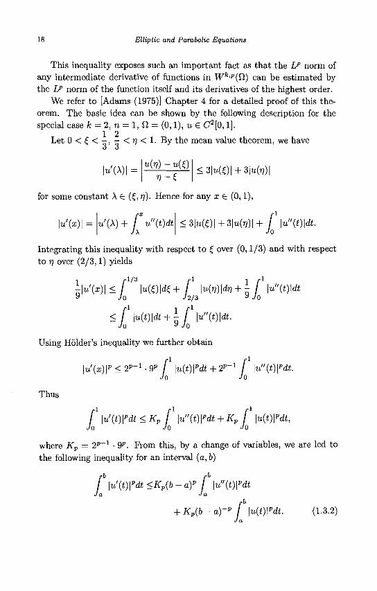
This inequality exposes such an important fact as that the IP norm of any intermediate derivative of functions in Wk'p(Q) can be estimated by the IP norm of the function itself and its derivatives of the highest order.
We refer to [Adams (1975)] Chapter 4 for a detailed proof of this theorem. The basic idea can be shown by the following description for the special case k = 2, n = 1, 9, = (0,1), u € C2[0,1].
1 2 Let 0 < £ < - , - < ? 7 < l . By the mean value theorem, we have
|u'(A)| = u{r)) - u{£)
ri-Z <3|u(0|+3|uft)|
for some constant A £ (£, rf). Hence for any x G (0,1),
\u'{x)\ = i'(X)+ f u"{t)dt <3|«(OI+3|«(»?) |+ / \u"{t)\dt. J\ Jo
Integrating this inequality with respect to £ over (0,1/3) and with respect to J] over (2/3,1) yields
\\v!{x)\ < [13\u(0\d£+ [ Wrj)\dr,+ \ f \u"(t)\dt 9 Jo J2/3 9 Jo
< f \u{t)\dt + \ f \u"{t)\dt. Jo 9 Jo
Using Holder's inequality we further obtain
\u'(x)\p<2p-1-9p [ \u(t)\pdt + 2p~1 [ \u"{t)\pdt. Jo Jo
Thus
/ \u'(t)\"dt<Kp [ \u"{t)\pdt + Kp f \u{t)\pdt, Jo Jo Jo
where Kp = 2P~1 • 9P. From this, by a change of variables, we are led to the following inequality for an interval (a, 6)
I \u'{t)\pdt<Kp(b-a)p f \u"(t)\pdt J a J a
+ Kp(b-a)-p f \u(t)\pdt. (1.3.2) J a
Preliminary Knowledge 19
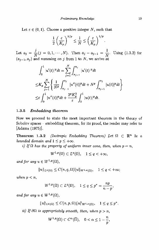
Let e € (0,1). Choose a positive integer N, such that
i /p 1 , 2 1 (~
\KP/
VP !
) ^ ' f £
U P 7 1
Let aj = j^(j = 0,1,--- ,N). Then Oj - Oj_i = —. Using (1.3.2) for (flj-i, flj) and summing on j from 1 to N, we arrive at
r1 N rai \ \u'(t)\pdt = Y^ / \u'(t)\pdt
JO j = l ^ a 3 - l
^ p E J ^ r wwdt+w n \u(t)\pdt) <£ / |u"(i)|Prfi+ £ / |lx(i)|P<i£.
Jo £ Jo
1.3.5 Embedding theorem
Now we proceed to state the most important theorem in the theory of Sobolev spaces - embedding theorem, for its proof, the reader may refer to [Adams (1975)].
Theorem 1.3.2 (Isotropic Embedding Theorem) Let ft c R" be a bounded domain and 1 < p < +oo.
i) If fi has the property of uniform inner cone, then, when p = n,
Wl'p{£l) c Lq(Q), l<q< +oo,
and for any u e Wl'p{£l),
IMUnn) < C(n,q,Q,)\\u\\wi,v(a), l<q< +co;
when p < n,
Wl'p{9) c L«(n), l < ? < p * = np
n—p
and for any u € WX'P{£1),
IMU«(fi) < C(«,P, n) | |u | |w i ,P (n), 1 < ^ < p*
ii) If <9f2 is appropriately smooth, then, when p > n,
W1,p(ft) c Ca(U), 0 < a < l - - ,
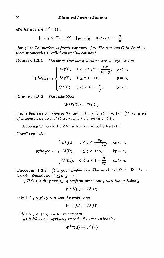
20 Elliptic and Parabolic Equations
and for any u € W1,p(fl),
\u\a;n < C(n,p,Q)\\u\\wi,p(n), n
0 < a < l - - . V
Here p* is the Sobolev conjugate exponent of p. The constant C in the above three inequalities is called embedding constant.
Remark 1.3.1 The above embedding theorem can be expressed as
W1 'p(fi)
' L«(fi), l<q<p* =
Lq(fl), 1 < q < +oo,
np n — p'
Ca(n), 0 < a < l - - , P
p<n,
p = n,
p> n.
Remark 1.3.2 The embedding
whp(n) «-> ca{U),
means that one can change the value of any function of W1,p(ft) on a set of measure zero so that it becomes a function in Ca(Cl).
Applying Theorem 1.3.2 for k times repeatedly leads to
Corollary 1.3.1
' L«(fi), 1 < q <
Wk'p(Q) e-> <
np kp < n, n — kp'
Lq(Cl), 1 < q < +oo, kp = n,
Ca(Ti), 0<a<l-^, kp>n. kp
Theorem 1.3.3 (Compact Embedding Theorem) Let il C W1 be a bounded domain and 1 < p < +oo.
i) If Q, has the property of uniform inner cone, then the embedding
Whp(£l) --» Lq(Sl)
with l<q<p*,p<n and the embedding
W1'"^) «-» Lq(Q)
with 1 < q < +oo, p = n are compact. ii) If dQ, is appropriately smooth, then the embedding
whp(n)^ca{ty
Preliminary Knowledge 21
ft
with p>n, 0<a<l is compact. P
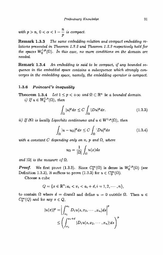
Remark 1.3.3 The same embedding relation and compact embedding relations presented in Theorem 1.3.2 and Theorem 1.3.3 respectively hold for the spaces Wo'p(n). In this case, no more conditions on the domain are needed.
Remark 1.3.4 An embedding is said to be compact, if any bounded sequence in the embedded space contains a subsequence which strongly converges in the embedding space, namely, the embedding operator is compact.
1.3.6 Poincare's inequality
Theorem 1.3.4 Let 1 < p < +oo and Q C M.n be a bounded domain. i) Ifu£Wl<p{Q), then
f \u\pdx < C [ \Du\pdx. (1.3.3) Jn Jn
ii) If dQ, is locally Lipschitz continuous and u G W1,p(fi), then
I \u- un\pdx <C I \Du\pdx (1.3.4)
Jn Jn with a constant C depending only on n, p and Q, where
un=mLu{x)dx
and |f2| is the measure ofQ.
Proof. We first prove (1.3.3). Since Cg°(fi) is dense in WQ'P{Q) (see Definition 1.3.3), it suffices to prove (1.3.3) for u € Cg°(fi).
Choose a cube
Q - {x€Rn;ai<Xi <ai+d,i-1,2,-•• , n} ,
to contain fi where d = diamfi and define u = 0 outside Q. Then u £ Co°(Q) and for any x £ Q,
\u(x)\p = / Diu(s,x2,-- • ,xn)ds Jai
(£ 1-a.i+d \ P
< I / \Diu(s,x2,--- ,xn)\ds
22 Elliptic and Parabolic Equations
<<F-1 f ' \D1u(s,x2,--- ,xn)\pds.
Integrating over Q leads to
f \u(x)\pdx = [ \u{x)\pdx Jn JQ
r rai+d <dP-x / / |Diu(s ,X2, • • • ,xn)\
pdsdx JQ Jax
<dp \ | D i u ( x i , i 2 . - " ,xn)\pdx
JQ
<dp f \Du\pdx, JQ
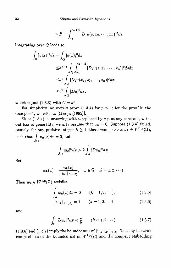
which is just (1.3.3) with C = dp. For simplicity, we merely prove (1.3.4) for p > 1; for the proof in the
case p = 1, we refer to [Maz'ja (1985)]. Since (1.3.4) is unvarying with u replaced by u plus any constant, with
out loss of generality, we may assume that UQ = 0. Suppose (1.3.4) failed, namely, for any positive integer k > 1, there would exists Uk £ W1'p(Cl),
such that / Uk(x)dx = 0, but Jn
f \uk\pdx >k [ \Duk\
pdx. Jn Jn
Set
wk{x) = llufc||LP(n)
Then wk G W1,p(fi) satisfies
/ Wk(x)dx = 0 Jn
IkfclUp(n) = 1
and
J \Dwk\pdx < i
xeii (fe = i ,2,---)-
(fc = l ,2 , - - - ) ,
(fc = l ,2,---)
(fc = l ,2 , - - - ) .
(1.3.5)
(1.3.6)
(1.3.7)
(1.3.6) and (1.3.7) imply the boundedness of ||i«fc||wi.j>(fi)- Thus by the weak compactness of the bounded set in W1,p(fi) and the compact embedding
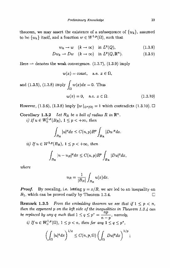
Preliminary Knowledge 23
theorem, we may assert the existence of a subsequence of {wk}, assumed to be {wk} itself, and a function w G W1,p(fi), such that
wk — w {k-^oo) in LP{Q), (1.3.8)
Dwk^Dw (fc-+oo) inL p (Q,R n ) . (1.3.9)
Here —*• denotes the weak convergence. (1.3.7), (1.3.9) imply
w(x) = const, a.e. x G Cl,
and (1.3.5), (1.3.8) imply / w(x)dx = 0. Thus
w(x) = 0, a.e. l e t l . (1.3.10)
However, (1.3.6), (1.3.8) imply ||w|U"(n) = 1 which contradicts (1.3.10). •
Corollary 1.3.2 Let BR be a ball of radius R in R™. i) Ifue WQ'P(BR), 1 < p < +oo, then
f \u\pdx < C(n,p)Rp f \Du\pdx. JBR JBR
ii) Ifu& Wl<p{BR), l<p< +oo, then
I \u-uR\pdx<C(n,p)Rp I \Du\pdx, JBR JBR
where
= \k Lu{x)dx-UR 'BR
Proof. By rescaling, i.e. letting y = x/R, we are led to an inequality on Bi, which can be proved easily by Theorem 1.3.4. •
Remark 1.3.5 From the embedding theorem we see that if 1 < p < n, then the exponent p on the left side of the inequalities in Theorem 1.3.4 can
TIT) be replaced by any q such that 1 < q < p* = , namely,
n — p i)Ifu£ WQ'P{Q), \<p<n, then for any 1 < q < p*,
( J \u\"dx\ < C{n,p, il)(f \Du\pdx\ ;
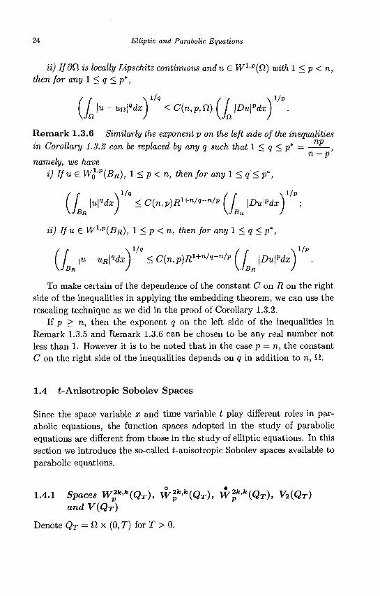
24 Elliptic and Parabolic Equations
ii) IfdQ. is locally Lipschitz continuous andu G W1,p(£l) with 1 < p < n, then for any 1 < q < p*,
([\u-uu\qdx) <C(n,p,Q)(f \Du\pdx\ ".
Remark 1.3.6 Similarly the exponent p on the left side of the inequalities 717)
in Corollary 1.3.2 can be replaced by any q such that 1 < q < p* = n — p namely, we have
i)Ifue WQ'P(BR), \<p<n, then for any 1 < q < p*,
(f \u\"dx) <C(n,p)R}+nlq-nlp(f \Du\pdx\ P ;
ii) IfuG W1'P(BR), 1 < p < n, then for any 1 < q < p*,
(I \u-uR\qdx] <C{n,p)R1+n/q-n/p( f \Du\pdx" \JBR J \JBR J
To make certain of the dependence of the constant C on R on the right side of the inequalities in applying the embedding theorem, we can use the rescaling technique as we did in the proof of Corollary 1.3.2.
If p > n, then the exponent q on the left side of the inequalities in Remark 1.3.5 and Remark 1.3.6 can be chosen to be any real number not less than 1. However it is to be noted that in the case p = n, the constant C on the right side of the inequalities depends on q in addition to n, fi.
1.4 t-Anisotropic Sobolev Spaces
Since the space variable x and time variable t play different roles in parabolic equations, the function spaces adopted in the study of parabolic equations are different from those in the study of elliptic equations. In this section we introduce the so-called t-anisotropic Sobolev spaces available to parabolic equations.
1.4.1 Spaces W™>k(QT), W2p
k'k(QT), Wf^iQx), V2{QT) and V(QT)
Denote QT = Q x (0, T) for T > 0.
Preliminary Knowledge 25
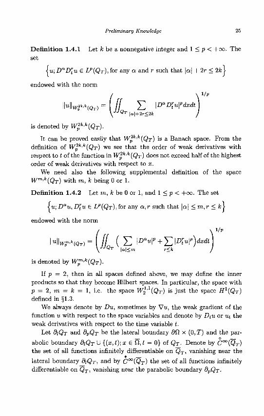
Definition 1.4.1 Let A; be a nonnegative integer and 1 < p < +oo. The set
iu; DaDrtu £ Lp(QT),ioi any a and r such that \a\ +2r < 2k\
endowed with the norm
Mw^{QT)=([[ E \DaD\u\^dxdt\ \JJQT \a\+2r<2k /
is denoted by W%k>k{QT).
It can be proved easily that Wpk'k{QT) is a Banach space. From the
definition of Wpk'k(Qr) we see that the order of weak derivatives with respect to t of the function in Wpk'k(Qr) does not exceed half of the highest order of weak derivatives with respect to x.
We need also the following supplemental definition of the space Wm'k(QT) with m, k being 0 or 1.
Definition 1.4.2 Let m, k be 0 or 1, and 1 < p < +oo. The set
<u;Dau,D\u € LP(QT),for any a,r such that \a\ <m,r<k>
endowed with the norm I/P
llUHwpm ' 'c(Q7-) = ( / / ( E \Dau\*+ Y,\Dtu\p)dxdt\
\JJQT | a | < m r<k J
is denoted by W™>k{QT).
If p = 2, then in all spaces denned above, we may define the inner products so that they become Hilbert spaces. In particular, the space with p = 2, m = k = 1, i.e. the space W2 ' {QT) is just the space H1(QT)
defined in §1.3. We always denote by Du, sometimes by Vu, the weak gradient of the
function u with respect to the space variables and denote by Dtu or ut the weak derivatives with respect to the time variable t.
Let BIQT and dpQr be the lateral boundary 9fi x (0,T) and the par
abolic boundary diQr U {(x,t);x £ Q, t = 0} of QT- Denote by C°°(QT) the set of all functions infinitely differentiable on QT, vanishing near the
• lateral boundary diQr, and by C°°(QT) the set of all functions infinitely differentiable on QT, vanishing near the parabolic boundary dpQx-
26 Elliptic and Parabolic Equations
Definition 1.4.3 Denote by W lk'k(Qr) the closure of C °°(QT) i n
Wpfc,fe(<9r); by W™'k(QT) with m, fc being 0 or 1 the closure of C°°(QT)
in Wp>k(QT); by W2fc'fc(Qr) t h e c l o s u r e o f c°°(QT) in W2fe>fc(QT); by
WP'k(QT) with m, fc being 0 or 1 the closure of C°°(QT) in W™<k(QT).
Definition 1.4.4 Let L°°(0,T; L2(£l)) be the set of all functions u such that for almost all t € (0,T), u(-,t) € L2(Cl) with ||u(-,t)||L2(n) bounded. Denote by V2(QT) the set L°°(0,T;L2(ft)) n W2
1 , 0(<2T) endowed with the norm
l lu l lv2(QT) = SUp \\u(-,t)\\L2{n)+ ( / / |Du| 2 otect t 0<t<T \JJQT
One may verify that V2(QT) is a Banach space.
Definition 1.4.5 Denote
V(QT) = {u &W^\QT)\Dut e L2(QT;^n)} ,
and define the inner product as
(U,V)V{QT) = (U,V)WI,I{QT) + {DuuDvt)L2(QT).
It is easy to prove
Proposition 1.4.1 V{QT) is dense in W2' (QT)-
Remark 1.4.1 W^'X(QT) can be regarded as the closure in W2' (QT), of the set of all infinitely differentiable functions on QT, vanishing near the bottom Q x {t = 0}.
1.4.2 Embedding theorem
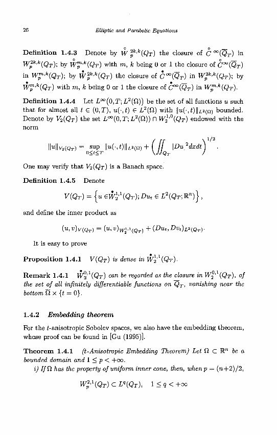
For the ^-anisotropic Sobolev spaces, we also have the embedding theorem, whose proof can be found in [Gu (1995)].
Theorem 1.4.1 (t-Anisotropic Embedding Theorem) Let Q C M.n be a bounded domain and 1 < p < +oo.
i) If CI has the property of uniform inner cone, then, whenp = (n+2)/2,
j . / i
Wl'\QT) C L«(QT), l<q<+oo
Preliminary Knowledge 27
and for any u £ WP'1(QT))
ML"(QT) < C(n,q,QT)\\u\\W2,i{QT),
when p < (n + 2)/2,
Wp2ll(Qr) C L«(QT), 1 < Q <
and for any u e W^,X{QT),
1 < q < +oo;
(n + 2)p
IMU'CQT) < C(".P>QT)||w||,yp2.1(QT)> 1 < Q <
is appropriately smooth, then, when p 5
W £ ' 1 ( Q T ) c C a , a / 2 ( Q r ) , 0 < a < 2
n + 2 - 2p
(n + 2)p n + 2 - 2p
uj 7/<9fi is appropriately smooth, then, when p> (n + 2)/2,
n + 2
P
and /or any u G Wp'^Qr) ,
Ma,a/2;QT < C(n,p, QT)\\U\\W2,I{QT), 0 < a < 2 n + 2
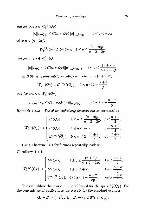
Remark 1.4.2 TTie a&ove embedding theorem can be expressed as
L"(QT),
Wl>l{QT)
x <,<_(!!+%, p < " + 2
n + 2 - 2p
^ ( Q r ) , 1 < < 7 < + C O , p =
2 ' n + 2
2 '
Using Theorem 1.4.1 for k times repeatedly leads to
Corollary 1.4.1
(n + 2)p
^ ' " ( Q T ) ^ -
£ " ( Q T ) ,
L"(QT),
1 <<?< kp <
Ca'a/2{QT), 0<a<2
n + 2-2kp
1 < q < +oo, kp =
n + 2 kp
kp >
n + 2 ~ 2 ~ ' n + 2 ~2~' n + 2
The embedding theorem can be established for the space V^Qr)- For the convenience of applications, we state it for the standard cylinder
Qp = Bpx(-p2,p2), Bp = {x e Rn; \x\ < p).
28 Elliptic and Parabolic Equations
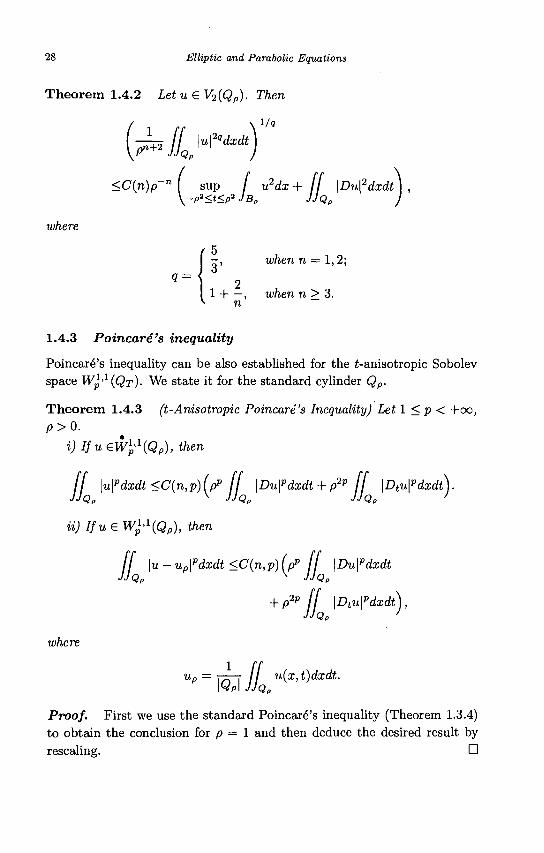
Theorem 1.4.2 Let u € V2(QP). Then
<C(n)p-n ( sup / u2dx + ff \Du\2dxdt \-p2<t<P
2 JBP JJQP ,
where
5 - , when n = 1,2;
«=\* 2 1 H—, when n > 3.
n
1.4.3 Poincare's inequality
Poincare's inequality can be also established for the ^-anisotropic Sobolev space Wp'l{Qx)- We state it for the standard cylinder Qp.
Theorem 1.4.3 (t-Anisotropic Poincare's Inequality) Let 1 < p < +co,
p>0.
i) Ifu£Wl/{QP), then
ff \u\pdxdt<C(n,p)(pr [J \Du\pdxdt + p2p [J \Dtu\pdxdt).
ii) IfueW^iQp), then
[f \u-up\pdxdt<C(n,p)(pp ff \Du\pdxdt
+ p2p ff \Dtu\pdxdt\
where
Up = - r - r / / u(x, t)dxdt. \Qp\ JJQp
Proof. First we use the standard Poincare's inequality (Theorem 1.3.4) to obtain the conclusion for p = 1 and then deduce the desired result by rescaling. •
Preliminary Knowledge 29
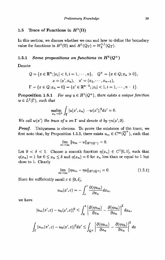
1.5 Trace of Functions in f f x ( f i )
In this section, we discuss whether we can and how to define the boundary value for functions in ff^fi) and Hl(QT) = W^iQr)-
1.5.1 Some propositions on functions in fl"1(Q+)
Denote
Q = {x G E n ; \xi\ < 1, i = 1, • • • , n), Q+ = {x G Q; xn > 0},
•E = v-^ > Xn), X = (Xi, • • • , Xn—\ ) ,
r = { x £ Q ; i „ = 0} = {x' G Rn_1; \xi\ < 1, i = 1, • • • , n - 1}.
Proposition 1.5.1 For any u € i f 1 (Q + ) , there exists a unique function w G L2(T), such that
esslim / \u(x',xn) — w(x')\2dx' = 0.
We call w(x') the trace of u onT and denote it by *yu(x',0).
Proof. Uniqueness is obvious. To prove the existence of the trace, we first note that, by Proposition 1.3.3, there exists um G C°°(Q ), such that
lim | |um- t i | | i f i (Q+) = 0 . m—>oo v '
Let 0 < S < 1. Choose a smooth function r](xn) G CJ[0,1], such that v(xn) = 1 for 0 < xn < 6 and r)(xn) = 0 for xn less than or equal to 1 but close to 1. Clearly
lim \\r}Um-r)u\\Hi{Q+) = 0 .
Since for sufficiently small e G [0,6],
rl d{r)um)
(1.5.1)
J£ dxn
we have
\um(x',e) -uk(x',e)\2 < / Jo
d(r)um) d(r)uk) OXfi CsXfi
QjXji)
/ \um(x',e) -uk(x',e)\2dx' < l JY JQ+
d(yum) _ d(rjuk) UXJI UXJI
dx
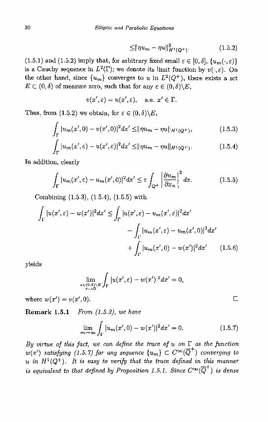
30 Elliptic and Parabolic Equations
<lfo«m-»Hffl(Q+)- (L 5-2)
(1.5.1) and (1.5.2) imply that, for arbitrary fixed small e G [0,5], {um(-, s)} is a Cauchy sequence in L2(T); we denote its limit function by v(-,e). On the other hand, since {um} converges to u in L2(Q+), there exists a set E c (0,5) of measure zero, such that for any e € (0, S)\E,
v(x',e) = u(x',e), a.e. x' S T.
Thus, from (1.5.2) we obtain, for e € {0,5)\E,
/ \um(x',0)-v(x',0)\2dx'<\\r)um-'nu\\Hi{Q+), (1.5.3)
/ \um{x',e) -u(x',e)\2dx' <\\rjum -r]u\\HHQ+). (1.5.4) /r
In addition, clearly 2
dx. (1.5.5) / |um(a;/,e) - um(x ' ,0) |2dx' < e 1 Jr Jo
du„ 0xn
Combining (1.5.3), (1.5.4), (1.5.5) with
/ \u(x',e) — w(x')\2dx' < / \u(x',e) — um(x',e)\2dx'
+ / \um(x',e) -um(x',0)\2dx'
+ f \um(x',0)-w(x')\2dx' (1.5.6)
yields
lim / \u(x',s) — w(x')\2dx' = 0, B(0,S)\E Jr e€(0,S)\E Jr
£ - . 0
where w{x') = v(x',0). D
Remark 1.5.1 From (1.5.3), we have
lim / \um(x', 0) - w{x')\2dx' = 0. (1.5.7)
By virtue of this fact, we can define the trace of u on V as the function w(x') satisfying (1.5.7) for any sequence {um} C C°°(Q ) converging to u in H1(Q+). It is easy to verify that the trace defined in this manner is equivalent to that defined by Proposition 1.5.1. Since C°°(Q ) is dense
Preliminary Knowledge 31
in C1(Q ) , we can replace the sequence {um} in formula (1.5.7) by any
sequence in C1(Q ) , converging to u in H1(Q+).
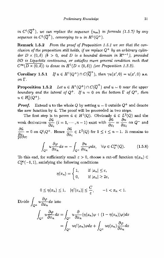
R e m a r k 1.5.2 From the proof of Proposition 1.5.1 we see that the conclusion of the proposition still holds, if we replace Q+ by an arbitrary cylinder D x (0,5) (8 > 0, and D is a bounded domain in R™-1j, provided 3D is Lipschitz continuous, or satisfies more general condition such that C°°(Dx (0,6)) is dense in HX(D x (0,5)) (see Proposition 1.3.3).
Corollary 1.5.1 If u & Hl(Q+) n C(Q + ) , then ju(x',0) = u(x\0) a.e. onT.
Proposi t ion 1.5.2 Let u G Hl(Q+) fl C(Q ) and u = 0 near the upper boundary and the lateral of Q+. If u = 0 on the bottom T of Q+, then u£Hl(Q+).
Proof. Extend u to the whole Q by setting u = 0 outside Q+ and denote the new function by u. The proof will be proceeded in two steps.
The first step is to prove u G H1(Q). Obviously u £ L2(Q) and the , , . . 9u .. , v . . , du du _ ,
weak derivatives —— (i = 1, • • • , n — 1) exist with —— = —— on Q~*~ and axi axi axi
du CJU —— = 0 on Q\Q+. Hence —— € L2(Q) for 1 < i < n — 1. It remains to axi axi prove
f u^Ldx = _ f |%<fa , W> e C?(Q). (1.5.8) JQ+ OXn JQ+ OXn
To this end, for sufficiently small e > 0, choose a cut-off function rj(xn) G CQ°(—1,1), satisfying the following conditions
V[Xn) ^ i f | , „ | > 2 £ ,
0 < r)(x„) < 1, |i7'(ar„)| < - , - 1 < xn < 1.
d<p Divide / u——dx into
IQ+ OX. JQ+U<-
/ u——dx = I u-—(r)(xn)<p + (1 - r)(xn))tp)dx JQ+ oxn JQ+ oxn
\ un'(xn)ipdx + / wq(xn)-—dx Jo+ JQ+ oxn
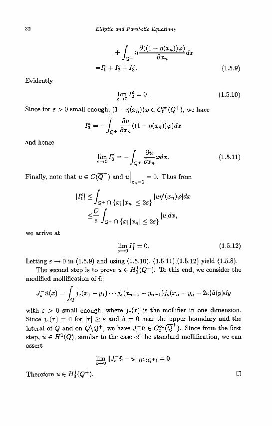
32 Elliptic and Parabolic Equations
JQ+ OXn
Evidently
=7f + 7f + 7f. (1.5.9)
lim7f = 0. (1.5.10)
Since for e > 0 small enough, (1 — r}(xn))<p € Co°(Q+), we have
i5 = -L^« 1-^-))^ and hence
lim 7 | / p-<pdx. (1.5.11)
Finally, note that u £ C(Q ) and u = 0 . Thus from lx „=0
|7f| < / |u77'(a;n)y>|da; VQ+ n {x; |x„| < 2e}
<2e} c r
<— / |u|da;, £ JQ+ r\{x;\xn\
we arrive at
l i m 7 f = 0 . (1.5.12)
Letting e -» 0 in (1.5.9) and using (1.5.10), (1.5.11),(1.5.12) yield (1.5.8). The second step is to prove u G 77o(Q+). To this end, we consider the
modified mollification of u:
J~u{x) = / je(xi - 3/1) • ••jeixn-i - yn-i)je{xn - Vn - 2e)u{y)dy JQ
with e > 0 small enough, where j e ( r ) is the mollifier in one dimension. Since js(r) = 0 for |r | > e and u = 0 near the upper boundary and the lateral of Q and on Q\Q+, we have J~u £ CQ°(Q ). Since from the first step, u £ H1(Q), similar to the case of the standard mollification, we can assert
lim \\J~u - u\\Hi(Q+) = 0.
Therefore u e 7701(Q+). D

Preliminary Knowledge 33
Proposition 1.5.3 Let u £ H1(Q+) n C(Q ) and u be the extension of
u to Q by setting u(x) = u(a;',0) on Q~ = Q\Q . Then u £ H1(Q).
Proof. The proof is just the same as the first step of the proof of Proposition 1.5.2, and the only difference is that here we need to require n{xn) to be an even function. •
1.5.2 Trace of functions in i f 1 ( f i )
Theorem 1.5.1 Let 0 C K™ be a bounded domain with smooth boundary. Then any u £ Hl(Sl) has trace ju on dQ, and ^u £ L2(dVt), namely, there exists a unique function ju £ L2(d£l) satisfying
lim m—+oo
/ \um - ju\2da = 0 (1.5.13) Jan
where {um} C C1(fi) is an arbitrary sequence converging to u in Hl{£l).
Proof. Since dfl is smooth, every point on dQ has a small neighborhood U, with the following property: there exists a smooth invertible mapping * , transforming Q = {y £ Rn; \yi\ < 1, i = 1, • • • , n} into U and Q+ = {y £ Q; yn > 0} into UnQ., such that * ( r ) = UndQ,, where T = {y £ Q; yn = 0}.
Let {um} C C1(fi) be an arbitrary sequence converging to u in H1^). Denote vm = {r)um) o * with n(x) £ C™(U). Then vm £ C^Q4") and vm = 0 near the upper boundary and the lateral of Q+ and
lim \\vm - (nu) o *||Hi(Q+) = 0. m—»oo ^ '
By Proposition 1.5.1, there exists h £ L2(T), such that
lim [\vm(y',0)-h(y')\2dy' = 0.
Obviously, h = 0 near the boundary of T. Returning to the variable x, we obtain
lim / \num — w\2do- = 0, m->°° Junan
where w = h o $ and $ = ($! , • • • , $ n ) is the inverse of \I>. Note *n(x)=0
w = 0 near the boundary of U (~l dQ,. After a zero-extension of w to dfl,
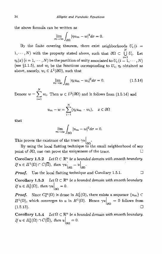
34 Elliptic and Parabolic Equations
the above formula can be written as
lim m^°° /an
/ \vum -JdCl
w\2da = 0.
By the finite covering theorem, there exist neighborhoods Ui (i = N
!,••• ,N) with the property stated above, such that dCl C \J U. Let
T)i(x) (i = 1, • • • ,N)be the partition of unity associated to U (i = 1, • • • ,N) (see §1.1.5), and Wi be the functions corresponding to Ui, Tji obtained as above, namely, w, € L2(dfl), such that
lim m—>oo
/ \Vium -Wi\2da = 0. (1.5.14) 'Jan
N
Denote w = 2_Jwi- Then w € L2(dCl) and it follows from (1.5.14) and
»=i
N
^2(Vium - W
that
Um—W
lim
x£d£l i = l
'JdCl \um — w\2da = 0.
dCl This proves the existence of the trace ju
By using the local flatting technique to the small neighborhood of any point of 9fi, one can prove the uniqueness of the trace. •
Corollary 1.5.2 Let Q C Rn be a bounded domain with smooth boundary.
Ifu£ H1^) n C(U), then ju =u an an
Proof. Use the local flatting technique and Corollary 1.5.1. • Corollary 1.5.3 Let fl c K " be a bounded domain with smooth boundary.
7 / t i e H&(Q.), then 7U = 0.
an
an
Proof. Since CQ°(Q) is dense in HQ(CI), there exists a sequence {um} C
771(f2), which converges to u in i?1(f2). Hence ju
(1.5.13).
Corollary 1.5.4 Let fl C Rn be a bounded domain with smooth boundary.
Ifu£ H£(Cl) n C(ty, then u = 0 . an
0 follows from
•
Preliminary Knowledge 35
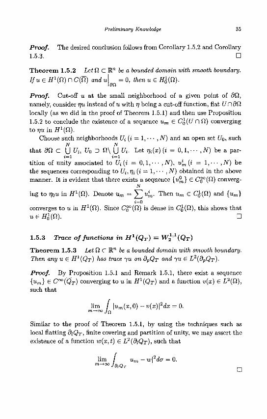
Proof. The desired conclusion follows from Corollary 1.5.2 and Corollary 1.5.3. •
Theorem 1.5.2 LetQ C Rn be a bounded domain with smooth boundary.
Ifue H\n) n C(fi) and u = 0 , then u € H&(n).
Proof. Cut-off u at the small neighborhood of a given point of dfl, namely, consider rju instead of u with 77 being a cut-off function, flat U D dQ, locally (as we did in the proof of Theorem 1.5.1) and then use Proposition 1.5.2 to conclude the existence of a sequence um € CQ(U (1 £1) converging to rju in ifx(Q).
Choose such neighborhoods Ui (i = 1, • • • , N) and an open set f/o, such JV N
that 9 f l c U Ui, U0 D fi\ |J t/i. Let r)i(x) (i = 0,1, • • • , TV) be a par-
tition of unity associated to Ui (i — 0, l,--- ,iV), ulm (i = l,--- ,N) be
the sequences corresponding to Ui, r]i (i = 1, • • • , N) obtained in the above manner. It is evident that there exists a sequence {u^} 6 Co°(fi) converg-
N
ing to T]QU in H1^). Denote um — ^2Kn- Then um G CQ(CI) and {um} i=0
converges to u in i?1(fi). Since C^(Q) is dense in CQ(CI), this shows that
1.5.3 Trace of functions in H1^) = Wl,x{QT)
Theorem 1.5.3 Let Q, (ZW1 be a bounded domain with smooth boundary. Then any u £ H1(QT) has trace ju on dpQr and ju € L2{dpQr)-
Proof. By Proposition 1.5.1 and Remark 1.5.1, there exist a sequence {um} € C°°(QT) converging to u in HX(QT) and a function v(x) £ L2(Cl), such that
m—+00 / lim / \um(x,0) — v(x)\2dx = 0.
Similar to the proof of Theorem 1.5.1, by using the techniques such as local flatting OIQT, finite covering and partition of unity, we may assert the existence of a function w(x,t) e L2(diQr), such that
lim / \um ~ w\2da = 0. m-*00JalQT
36 Elliptic and Parabolic Equations
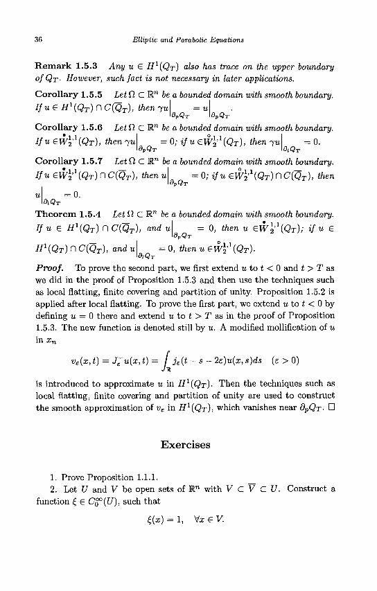
R e m a r k 1.5.3 Any u £ ^(QT) also has trace on the upper boundary ofQr- However, such fact is not necessary in later applications.
Corollary 1.5.5 Let Cl C Mn be a bounded domain with smooth boundary. IfuG H^QT) n C(QT), then 7 u
dpQi dpQj
Corollary 1.5.6 Let Cl C K" be a bounded domain with smooth boundary.
Ifu£W2' (QT), then-yu dpQi
0; ifu&WriQr), then ju diQT
= 0.
Corollary 1.5.7
ISUEW121{QT)^C(QT), thenu
= 0. 9iQT
Let Cl C R" be a bounded domain with smooth boundary.
= 0; ifu ewl^iQr) n C(QT), then dpQr
Theorem 1.5.4 Let Cl C R" be a bounded domain with smooth boundary.
Ifue Hl(QT) n C{QT), and u i , i /
9PQT 0, then u £W 2> (QT); if u €
H 1{QT) n C(QT), andu = 0 , then u <EW2 (QT)-dtQT
Proof. To prove the second part, we first extend u to t < 0 and t > T as we did in the proof of Proposition 1.5.3 and then use the techniques such as local flatting, finite covering and partition of unity. Proposition 1.5.2 is applied after local flatting. To prove the first part, we extend u to t < 0 by denning u = 0 there and extend u to t > T as in the proof of Proposition 1.5.3. The new function is denoted still by u. A modified mollification of u in xn
ve(x,t) = J~u(x,t) = / je(t — s - 2e)u(x,s)ds (e > 0) Ju
is introduced to approximate u in i f 1 (Qr)- Then the techniques such as local flatting, finite covering and partition of unity are used to construct the smooth approximation of v£ in ^(QT), which vanishes near OVQT- •
Exercises
1. Prove Proposition 1.1.1. 2. Let U and V be open sets of M" with V C V C U. Construct a
function £ £ C$°(U), such that
£(x) = 1, Vz € V.
Preliminary Knowledge 37
3. Prove Proposition 1.2.1. 4. Prove Corollary 1.2.1. 5. Judge whether W1,1(fi) is a Banach space, where Q C W1 is an open
set. 6. Prove Proposition 1.3.2. 7. Prove Propositions 1.3.8-1.3.10. 8. Let u G W1,p((0,1)) with p > 1. Prove
\u(x)-u(y)\ < | x - y | 1 _ 1 / p ( / |i/(*)|pcft) ", for almost all x,y G [0,1].
9. Let fi C R" be an open set, 1 < p < +oo and u G W1 'p(fi). i) Prove u+,u~ G W1-p(0), and
{ Du(x), whenever u(x) > 0,
0, whenever u(x) < 0,
Du(x), whenever u(x) < 0, Du"(a;) =
0, whenever u(x) > 0,
where
ii) Prove
u + = m a x { u , 0 } , u =min{tt, 0};
Du(x) = 0, a.e. x G {x G Q,; u(x) = 0}.
10. Prove Corollary 1.3.2 and Remark 1.3.6. 11. Prove Theorem 1.4.3. 12. Prove Proposition 1.5.3.

Chapter 2
L2 Theory of Linear Elliptic Equations
This chapter is devoted to the L2 theory of linear elliptic equations. We first present the argument for a typical equation, i.e. Poisson's equation thoroughly and then turn to the general equations in divergence form.
2.1 Weak Solutions of Poisson's Equation
Let fl C i n be a bounded domain with piecewise smooth boundary dtt. Consider the equation
- A u = / ( i ) (2.1.1)
in fi, where x = (xi, • • • , xn), A is Laplace operator in n dimension, i.e.
A - — — — dx\ dx\ dx%
and / € L2(Q,). For simplicity, we merely discuss the Dirichlet problem for equation (2.1.1) with the homogeneous boundary value condition
= 0. (2.1.2) an v '
If a nonhomogeneous boundary value condition
= g(x) (2.1.3) oil
is assumed with g{x) appropriately smooth on Q, then we can transform the problem into the one with the homogeneous boundary value condition by considering the equation for u(x) — g(x), which is still a Poisson's equation with another function as its right member.
39
40 Elliptic and Parabolic Equations
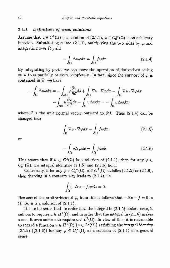
2.1.1 Definition of weak solutions
Assume that u £ C2(Cl) is a solution of (2.1.1), ip £ CQ°(Q.) is an arbitrary function. Substituting u into (2.1.1), multiplying the two sides by tp and integrating over Q yield
- / Ampdx = / fipdx. (2-1.4) Jn Jn
By integrating by parts, we can move the operation of derivatives acting on u to ip partially or even completely. In fact, since the support of <p is contained in fi, we have
- / Autpdx = — I (p-^ds + / Vu • Vipdx = I Vu- Vipdx Jn Jan vv Jn Jn
— \ u—^ds — I uAipdx = — I uAipdx, Jdn vv Jn Jn
where V is the unit normal vector outward to dQ,. Thus (2.1.4) can be changed into
/ Vu-V</>dz= / fipdx (2.1.5) Jn Jn
or
- / uAipdx = / fipdx. (2.1.6) Jn Jn
This shows that if u € C2(Q) is a solution of (2.1.1), then for any (p € Co°(fi), the integral identities (2.1.5) and (2.1.6) hold.
Conversely, if for any ip e Cg°(n), u € C2(fi) satisfies (2.1.5) or (2.1.6), then deriving in a contrary way leads to (2.1.4), i.e.
/ ( -Au - f)tpdx = 0. Jn
Because of the arbitrariness of ip, from this it follows that — Au — / = 0 in Q, i.e. it is a solution of (2.1.1).
It is to be noted that, in order that the integral in (2.1.5) makes sense, it suffices to require u € / f 1 (0) , and in order that the integral in (2.1.6) makes sense, it even suffices to require u £ L2(tt). In view of this, it is reasonable to regard a function u £ Hl{Q) (u £ L2(f2)) satisfying the integral identity (2.1.5) ((2.1.6)) for any <p £ C^(fl) as a solution of (2.1.1) in a general sense.
L2 Theory of Linear Elliptic Equations 41
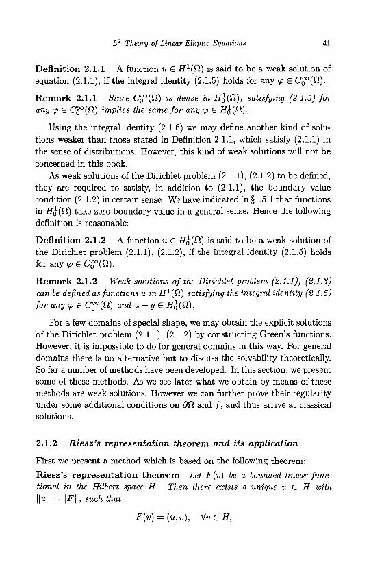
Definition 2.1.1 A function u £ i/1(fi) is said to be a weak solution of equation (2.1.1), if the integral identity (2.1.5) holds for any tp £ CQ°(Q).
R e m a r k 2.1.1 Since CQ°(Q) is dense in HQ(CI), satisfying (2.1.5) for any tp £ CQ°(£1) implies the same for any <p £ HQ(CI).
Using the integral identity (2.1.6) we may define another kind of solutions weaker than those stated in Definition 2.1.1, which satisfy (2.1.1) in the sense of distributions. However, this kind of weak solutions will not be concerned in this book.
As weak solutions of the Dirichlet problem (2.1.1), (2.1.2) to be denned, they are required to satisfy, in addition to (2.1.1), the boundary value condition (2.1.2) in certain sense. We have indicated in §1.5.1 that functions in HQ (Q) take zero boundary value in a general sense. Hence the following definition is reasonable:
Definition 2.1.2 A function u £ HQl(Q) is said to be a weak solution of
the Dirichlet problem (2.1.1), (2.1.2), if the integral identity (2.1.5) holds for any tp £ C^°(fi).
R e m a r k 2.1.2 Weak solutions of the Dirichlet problem (2.1.1), (2.1.3) can be defined as functions u in Hl(Q) satisfying the integral identity (2.1.5) for any tp £ Cg° (Q) and u — g £ HQ (Q).
For a few domains of special shape, we may obtain the explicit solutions of the Dirichlet problem (2.1.1), (2.1.2) by constructing Green's functions. However, it is impossible to do for general domains in this way. For general domains there is no alternative but to discuss the solvability theoretically. So far a number of methods have been developed. In this section, we present some of these methods. As we see later what we obtain by means of these methods are weak solutions. However we can further prove their regularity under some additional conditions on d£l and / , and thus arrive at classical solutions.
2.1.2 Riesz's representation theorem and its application
First we present a method which is based on the following theorem:
Riesz's representa t ion theorem Let F(v) be a bounded linear functional in the Hilbert space H. Then there exists a unique u £ H with ||u|| = H-FH, such that
F{v) = (u,v), \/v£H,
42 Elliptic and Parabolic Equations
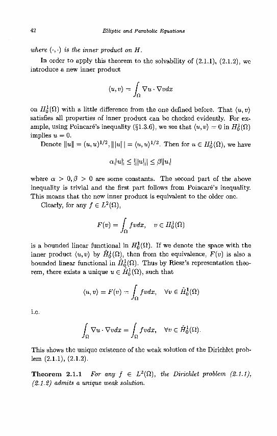
where (•, •) is the inner product on H.
In order to apply this theorem to the solvability of (2.1.1), (2.1.2), we introduce a new inner product
(u, v) = I Vu • Vvdx Jn
on HQ (fi) with a little difference from the one defined before. That (u, v) satisfies all properties of inner product can be checked evidently. For example, using Poincare's inequality (§1.3.6), we see that (u,v) = 0 in HQ(£1)
implies u = 0. Denote ||u|| = (u,u)1/2, \\\u\\\ = (u,^)1 /2 . Then for u G HQ(Q), we have
a | |u | |< | | | u | | |< /? | |u | |
where a > 0, f3 > 0 are some constants. The second part of the above inequality is trivial and the first part follows from Poincare's inequality. This means that the new inner product is equivalent to the older one.
Clearly, for any / G L2(Q.),
F(v) = f fvdx, v G Hb(Sl) Jn
is a bounded linear functional in HQ(£1). If we denote the space with the inner product {u,v) by HQ(Q), then from the equivalence, F(v) is also a bounded linear functional in HQ(Q). Thus by Riesz's representation theorem, there exists a unique u G HQ(£1), such that
(u,v) = F(v) = f fvdx, Vv G H%(Q.) Jn
i.e.
/ Vu • Vvdx = / fvdx, Vw G.#o(n)-Jn Jn
This shows the unique existence of the weak solution of the Dirichlet problem (2.1.1), (2.1.2).
Theorem 2.1.1 For any f G L2(Cl), the Dirichlet problem (2.1.1), (2.1.2) admits a unique weak solution.
L2 Theory of Linear Elliptic Equations 43
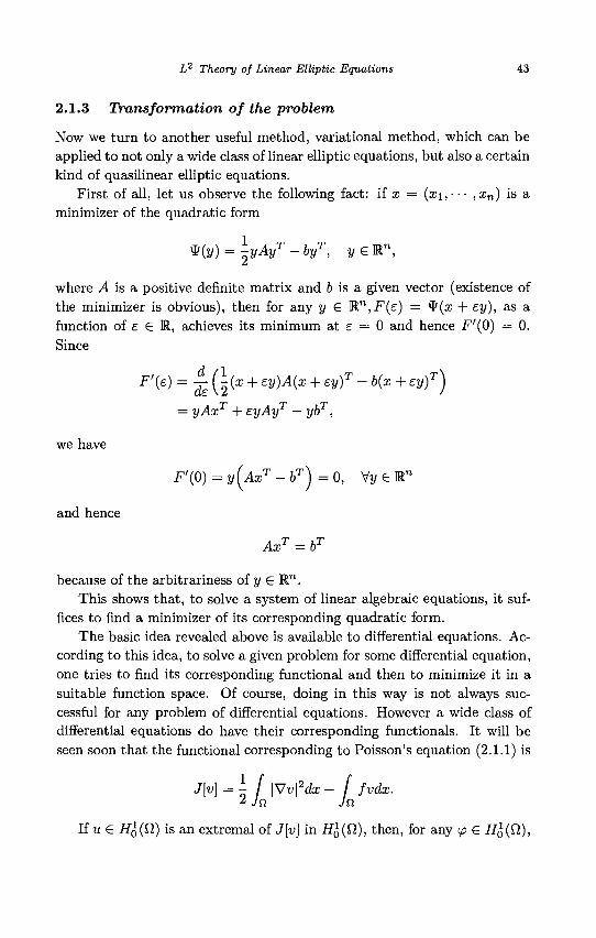
2.1.3 Transformation of the problem
Now we turn to another useful method, variational method, which can be applied to not only a wide class of linear elliptic equations, but also a certain kind of quasilinear elliptic equations.
First of all, let us observe the following fact: if x = (x\, • • • ,xn) is a minimizer of the quadratic form
y{y) = \yAyT -byT, yeRn,
where A is a positive definite matrix and 6 is a given vector (existence of the minimizer is obvious), then for any y £ M.n,F(e) = *(x + ey), as a function of £ S R, achieves its minimum at e = 0 and hence .F'(O) = 0. Since
F'(e) = ^ ( i ( x + ey)A(x + eyf - b(x + ey)T)
= yAxT + eyAyT - ybT,
we have
F'(0) = y(AxT-bT\ = 0 , V y e R "
and hence
AxT = bT
because of the arbitrariness of y € R™. This shows that, to solve a system of linear algebraic equations, it suf
fices to find a minimizer of its corresponding quadratic form. The basic idea revealed above is available to differential equations. Ac
cording to this idea, to solve a given problem for some differential equation, one tries to find its corresponding functional and then to minimize it in a suitable function space. Of course, doing in this way is not always successful for any problem of differential equations. However a wide class of differential equations do have their corresponding functionals. It will be seen soon that the functional corresponding to Poisson's equation (2.1.1) is
J¥\ = o / \^v\2dx - / fvdx-2 Ja Jo,
If u e HQ(fi) is an extremal of J[v] in HQ(Q), then, for any ip e HQ(£1),
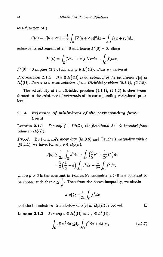
44 Elliptic and Parabolic Equations
as a function of e,
F(s) = J[u + e<p] = - / \V(u + e(p)\2dx- / f{u + etp)dx 2 Jn Jn
achieves its extremum at e = 0 and hence F'(0) = 0. Since
F'(e) = / (Vu + eV<p)V(pdx - \ f<pdx, Jn Jn
-F'(O) = 0 implies (2.1.5) for any tp € HQ(£1). Thus we arrive at
Proposition 2.1.1 Ifu £ HQ(Q,) is an extremal of the functional J[v] in #o(fi), then u is a weak solution of the Dirichlet problem (2.1.1), (2.1.2).
The solvability of the Dirichlet problem (2.1.1), (2.1.2) is then transformed to the existence of extremals of its corresponding variational problem.
2.1.4 Existence of minimizers of the corresponding functional
Lemma 2.1.1 For any f £ L2(Q), the functional J[v] is bounded from below in HQ(Q,).
Proof. By Poincare's inequality (§1.3.6) and Cauchy's inequality with e (§1.1.1), we have, for any v € HQ(£1),
-5(Hi>-s//* where fx > 0 is the constant in Poincare's inequality, e > 0 is a constant to
be chosen such that e < —. Then from the above inequality, we obtain
JM>-^£Jnfdx
and the boundedness from below of J[v] in HQ(Q) ^s proved. •
Lemma 2.1.2 For any v € #o(fi) and f € L2(Q.),
f \Vv\2dx <4|U / f2dx + 4J[v], (2.1.7) Jn Jn
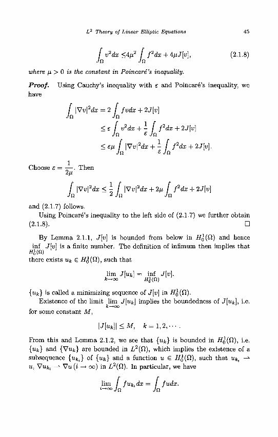
L2 Theory of Linear Elliptic Equations 45
/ v2dx <4/x2 f fdx + AfiJ[v], (2.1.8) Jn Jn
where n> 0 is the constant in Poincare's inequality.
Proof. Using Cauchy's inequality with e and Poincare's inequality, we have
/ \Vv\2dx = 2 1 fvdx + 2J[v] Jn Jn
: [ v2dx + - f fdx + 2J[v] Jn £ Jn
e\x f \Vv\2dx + - f fdx + 2J[v]. Jn £ Jn
<e
<
Choose e = — . Then 2/i
/ \Vv\2dx <\ I \Vv\2dx + 2/x / fdx + 2J\v] Jn 2 Jn Jn
and (2.1.7) follows. Using Poincare's inequality to the left side of (2.1.7) we further obtain
(2.1.8). •
By Lemma 2.1.1, J\v] is bounded from below in HQ(Q) and hence inf J[v] is a finite number. The definition of infimum then implies that
tf<i(n) there exists Uk £ HQ(Q,), such that
lim Jfitfcl = inf J\v\. k->oo ffi(fj)
{uk} is called a minimizing sequence of J[v] in HQ(Q,).
Existence of the li
for some constant M,
Existence of the limit lim J[uk] implies the boundedness of J[ufe], i.e. k~*oo
\J[uk}\<M, k = l,2,---.
From this and Lemma 2.1.2, we see that {uk} is bounded in HQ(Q), i.e. {uk} and {Vtifc} are bounded in L2(£l), which implies the existence of a subsequence {u^} of {uk} and a function u £ HQ(CI), such that uki —*• u, Vu^ —*• Vu(i —> oo) in L2(Q). In particular, we have
lim / fukdx = / fudx. i-"30 Jn Jn
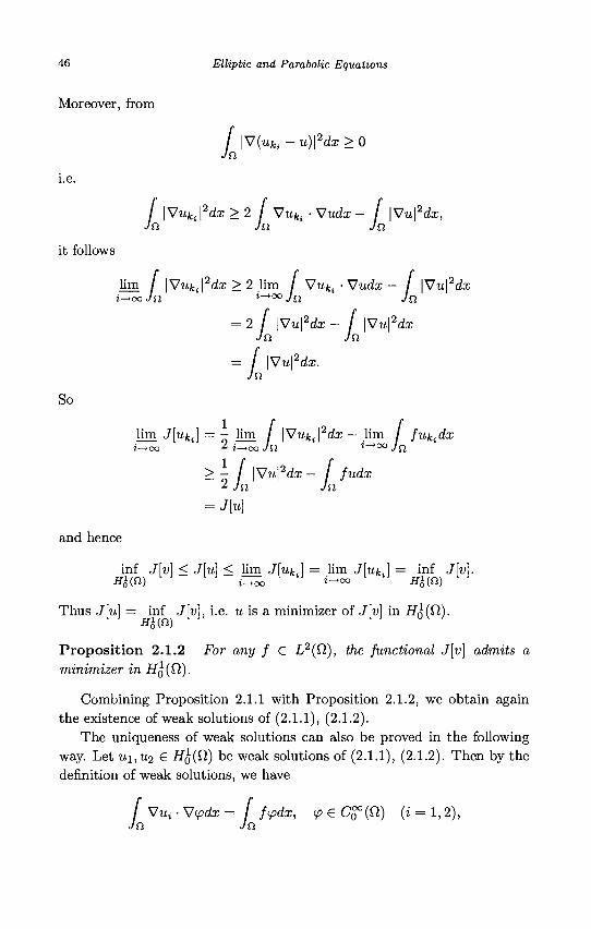
46 Elliptic and Parabolic Equations
Moreover, from
/ | V ( W / f c i - u ) | 2 ^ > 0 Jn
i.e.
/ \Vuki\2dx>2 \ Vuki-Vudx- / \S7u\2dx,
Jn Jn Jn
it follows
lim / \Vuki\2dx > 2 lim / Vuki-Vudx- / |Vu|2dx
*->oo Jn *->°° Jn Jn
= 2 / \Vu\2dx - f \X7u\2dx Jn Jn
f |Vu|: Jn
dx.
So
lim J[uki] — - lim / \Vuki\2dx - lim / fukidx
> - / |Vu|2cte - / /udz
= J[«]
and hence
inf J[v] < J[u] < lim J[uki] = lim JfufeJ = inf J[v}. HZ(Sl) i-^oo i-*00 H*(Sl)
Thus J[w] = inf J[v], i.e. u is a minimizer of J[v] in i?o(Q).
Proposition 2.1.2 For any f £ L2(Q), the functional J[v] admits a minimizer in HQ(Q).
Combining Proposition 2.1.1 with Proposition 2.1.2, we obtain again the existence of weak solutions of (2.1.1), (2.1.2).
The uniqueness of weak solutions can also be proved in the following way. Let ui,U2 £ HQ(Q) be weak solutions of (2.1.1), (2.1.2). Then by the definition of weak solutions, we have
f Vui • Vipdx = I f(pdx, <p G C£°(ft) (i = 1,2), Jn Jn
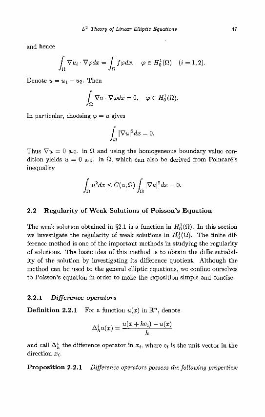
L2 Theory of Linear Elliptic Equations 47
and hence
/ Vui • V<pdx = / f(pdx, ip e H^(Q) (i = 1,2).
Denote u = u\ — u-2- Then
/ Vu • Vipdx = 0, <p £ H^(Q). Jn
In particular, choosing ip = u gives
7u\2dx = 0. / | V t
Thus Vu = 0 a.e. in Cl and using the homogeneous boundary value condition yields u = 0 a.e. in fi, which can also be derived from Poincare's inequality
/ u2dx < C(n,n) I |Vu|2ob = 0. Ja Jn
2.2 Regularity of Weak Solutions of Poisson's Equation
The weak solution obtained in §2.1 is a function in HQ(Q). In this section we investigate the regularity of weak solutions in HQ(Q). The finite difference method is one of the important methods in studying the regularity of solutions. The basic idea of this method is to obtain the differentiability of the solution by investigating its difference quotient. Although the method can be used to the general elliptic equations, we confine ourselves to Poisson's equation in order to make the exposition simple and concise.
2.2.1 Difference operators
Definition 2.2.1 For a function u(x) in Rn, denote
u(x + hei) — u(x) Alu(x) =
h
and call Alh the difference operator in xit where e* is the unit vector in the
direction xi.
Proposition 2.2.1 Difference operators possess the following properties:
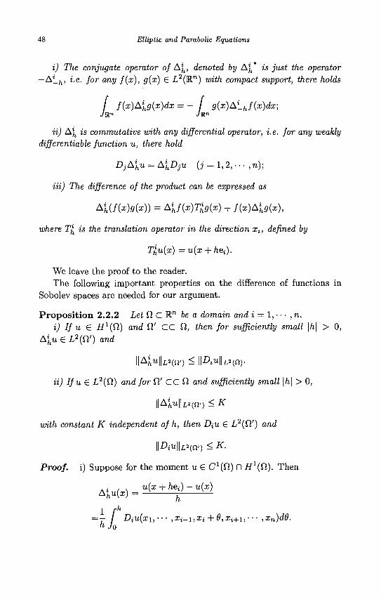
48 Elliptic and Parabolic Equations
i) The conjugate operator of Alh, denoted by Al
h is just the operator —Al_h, i.e. for any f(x), g(x) € L2(R") with compact support, there holds
[ f(x)Aihg{x)dx = - [ g(x)Alhf(x)dx;
ii) Alh is commutative with any differential operator, i. e. for any weakly
differentiable function u, there hold
DjAiu = AiDjU (j = l , 2 , . - . , n ) ;
Hi) The difference of the product can be expressed as
AUf(x)g(x)) = Ay(x)n9(x) + f(x)Aig(x),
where T£ is the translation operator in the direction Xi, defined by
Tlu{x) = u(x + hei).
We leave the proof to the reader. The following important properties on the difference of functions in
Sobolev spaces are needed for our argument.
Proposi t ion 2.2.2 Let fi C R™ be a domain and i = 1, • • • , n. i) If u £ /f1(f2) and Q.' CC 0 , then for sufficiently small \h\ > 0,
A ' ^ u e i 2 ^ ) and
\\&huh*(n') < \\Diu\\L2{n).
ii) IfuG L2(Q) and for fi' CC fi and sufficiently small \h\ > 0,
| |AU| | L 2 ( n 0 < K
with constant K independent of h, then DiU ۥ L2(Q') and
II Au||i*(n') < K.
Proof, i) Suppose for the moment u G Cl(Sl) n H1^). Then
u(x + he^ — u{x) a;«(x)
. r h
1 fh
- / Diu(xi,--- ,Xi-i,Xi + 0,Xi+i,--- ,xn)d6. h Jo
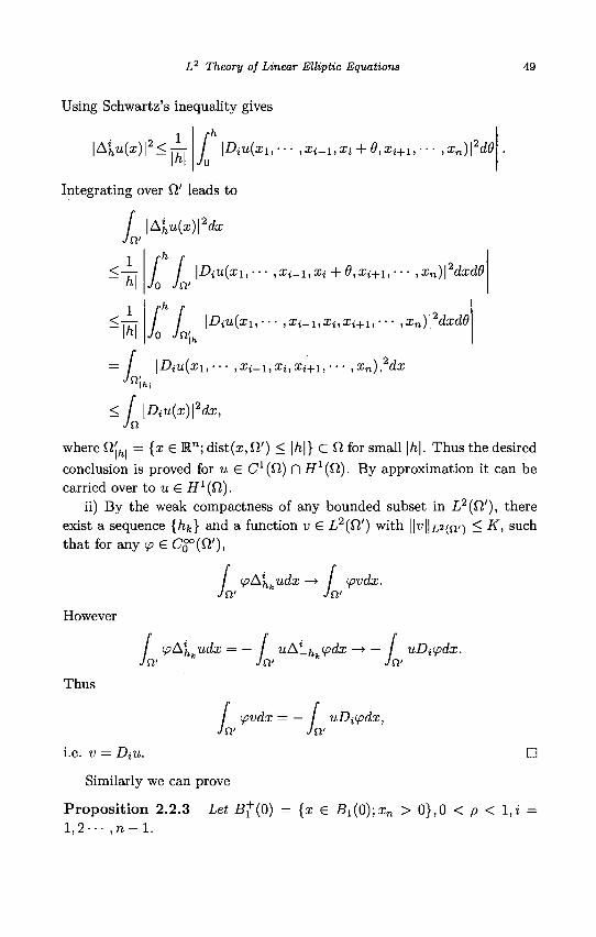
L2 Theory of Linear Elliptic Equations 49
Using Schwartz's inequality gives
rh
|A>(*)r< \h\ [ IA Jo
u(xi, • • • ,Xi-i,Xi +6,xi+i, • • • ,xn)\ dO
Integrating over fi' leads to
Whu{x)\2dx
2dxd6
/ / \Diu(xi,- •• ,Xi-i,Xi + 9,xi+i,-- • ,xn)\2dxd9
Jo JQ'
I I • i ' iW^Ii , • • • , 3^—1, Xi, Xj+ i , • • • ,Xn)\ Jo Jn>h]
< / \Diu(x)\2dx, Jn
where fi{h| = { i e Rn; dist(x, fi') < |/i|} c ft for small \h\. Thus the desired conclusion is proved for u G C1(fi) D /f1(Q). By approximation it can be carried over to u £ iJ1(fi).
ii) By the weak compactness of any bounded subset in L2(Q'), there exist a sequence {hk} and a function v G L2(0') with ||w||L2(n') < K, s u °h that for any <p G Cg°(Q')>
However
Thus
/ ipA}lkudx —> / ipvdx. Jo,1 Jw
/ <^A fcuda; = — I uAl_hkipdx —> — / uD^dx. Jci' J a1 Jo.1
/ <pt>d:r = — I uD{(pdx, Jw Jw
i .e. u = Z?jU.
Similarly we can prove •
Proposition 2.2.3 Lei -8^(0) = {a; G Bi(0);xn > 0},0 < p < l , i = 1,2--- , n - 1.
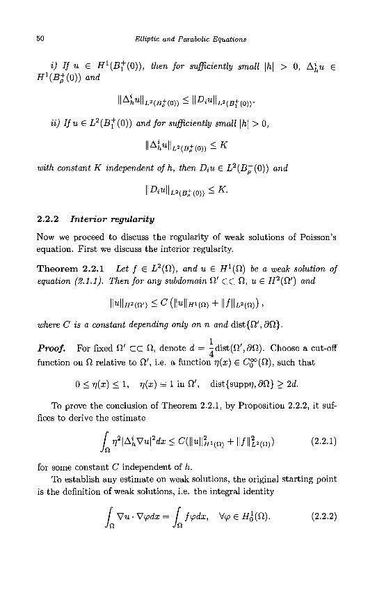
50 Elliptic and Parabolic Equations
i) If u G Hl(Bf(0)), then for sufficiently small \h\ > 0, A{u G H^B+iO)) and
HAfcullL»(B+(0» - WDiu\\mB+(0)y
ii) IfuE L2(Bf(0)) and for sufficiently small \h\ > 0,
II^UIIL2(B+(O)) ^ K
with constant K independent of h, then DiU G L2(B+(Q)) and
HAu|lz,2(B+(0)) ^ K-
2.2.2 Interior regularity
Now we proceed to discuss the regularity of weak solutions of Poisson's equation. First we discuss the interior regularity.
Theorem 2.2.1 Let f G L2(Q), and u G iJ:(ft) be a weak solution of equation (2.1.1). Then for any subdomain fi' CC fl, u € H2{Q.') and
\\U\\H'(Q') < C (||u||jfi(n) + H/Hz^n)),
where C is a constant depending only on n and dist{ft',9ft}.
Proof. For fixed ft' CC ft, denote d = -dist(ft',dft). Choose a cut-off
function on ft relative to ft', i.e. a function r](x) G Co°(ft), such that
0 < r}(x) < 1, rj(x) = 1 in ft', dist{suppr?, 9ft} > 2d.
To prove the conclusion of Theorem 2.2.1, by Proposition 2.2.2, it suffices to derive the estimate
/ Jn
V2\A{Vu\2dx < C(\\u\\2
H1{n) + | | / | |£ a ( n )) (2.2.1)
for some constant C independent of h. To establish any estimate on weak solutions, the original starting point
is the definition of weak solutions, i.e. the integral identity
/ Vu • Vydx = f fipdx, V<p G H%(Q). (2.2.2)
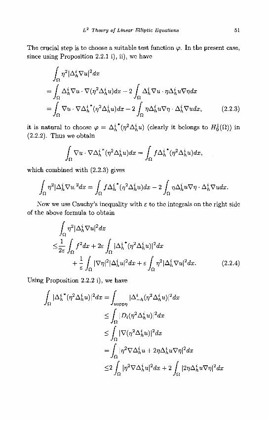
L2 Theory of Linear Elliptic Equations 51
The crucial step is to choose a suitable test function </?. In the present case, since using Proposition 2.2.1 i), ii), we have
L v2\AhVu\2dx
= f AhVu • V{ri2Ahu)dx -2 [ A\Vu • r/A^Vrycfo Jn Jn
= f Vw • VAi*(r)2Ahu)dx -2 [ TjA{uVr] • AhVudx, (2.2.3) Jn Jn
it is natural to choose cp = Azh*(rj2Al
hu) (clearly it belongs to HQ(Q,)) in (2.2.2). Thus we obtain
/ Vu • VAJ, V A ^ ) c f e = / fA\* (r,2Ahu)dx, Jn Jn
which combined with (2.2.3) gives
/ r)2\AhVu\2dx = f fAh*(r,2Ahu)dx - 2 / T / A ^ V T ? • A^Vudx. Jn Jn Jn
Now we use Cauchy's inequality with e to the integrals on the right side of the above formula to obtain
/ Jn
r,'\AhVu\'dx n
< ~2e
± [ f2dx + 2e [\Ak*(r,2Aiu)\2dx Z£ Jn Jn
+ - f \Vri\2\A\u\2dx + e / r ^ lA^Vul 2 ^ . (2.2.4) £ Jn Jn
Using Proposition 2.2.2 i), we have
/ \Ai*(V2Aiu)\2dx = f \Ath(v
2Aiu)\2dx
< / l A ^ A ^ ) ! 2 ^ Jn
< f \V(V2Ahu)\2dx
Jn
= [ I^VA^u + 2rjAiuVv\2dx Jn
<2 f \r]2VAiu\2dx + 2 / \2rjAhuVr]\2dx Jn Jn
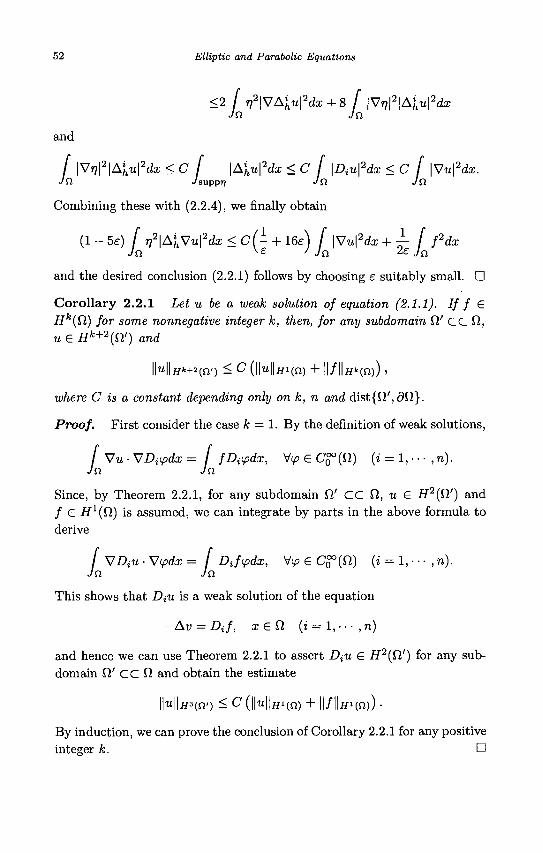
52 Elliptic and Parabolic Equations
<2 / r)2\VA{u\2dx + 8 [ |VT?|2|A^l2da?
Jo Jo
and
f |V»/|2|A£u|2da; < C f |A^r*|2da: < C f \DiU\2dx <C [ \Vu\2dx. JO ^supp7j JQ. JO
Combining these with (2.2.4), we finally obtain
(1 - 5e) / j j2 |A^V«|adi < C(- + l fe) / \Vu\2dx + ±- f fdx Jo v e ' Jo 2 £ Jo
and the desired conclusion (2.2.1) follows by choosing e suitably small. •
Corollary 2.2.1 Let u be a weak solution of equation (2.1.1). If f G Hk(Q) for some nonnegative integer k, then, for any subdomain Q' CC Cl, u G Hk+2(fl') and
IMU*+2(fi') < C (||u||Hi(n) + ||/||if=(n)) ,
where C is a constant depending only on k, n and dist{fi',9fi}.
Proof. First consider the case k = 1. By the definition of weak solutions,
/ Vu • VDupdx = / fDt(pdx, ty> G Cg°(n) (i = 1, • • • , n). Jo JO
Since, by Theorem 2.2.1, for any subdomain fi' CC Cl, u G H2(n') and / G if1 (£2) is assumed, we can integrate by parts in the above formula to derive
/ VDiU • \><pdx = I DJipdx, V<p G C§°(fi) (i = 1, • • • , n). Jo Jo,
This shows that DiU is a weak solution of the equation
-Av = Dif, xeQ. (i = l,---,n)
and hence we can use Theorem 2.2.1 to assert Dtu G H2(Q') for any sub-domain fi' CC O and obtain the estimate
l|w|k3(n') < C (|M|tfi(n) + ||/||ifi(n)) •
By induction, we can prove the conclusion of Corollary 2.2.1 for any positive integer k. •
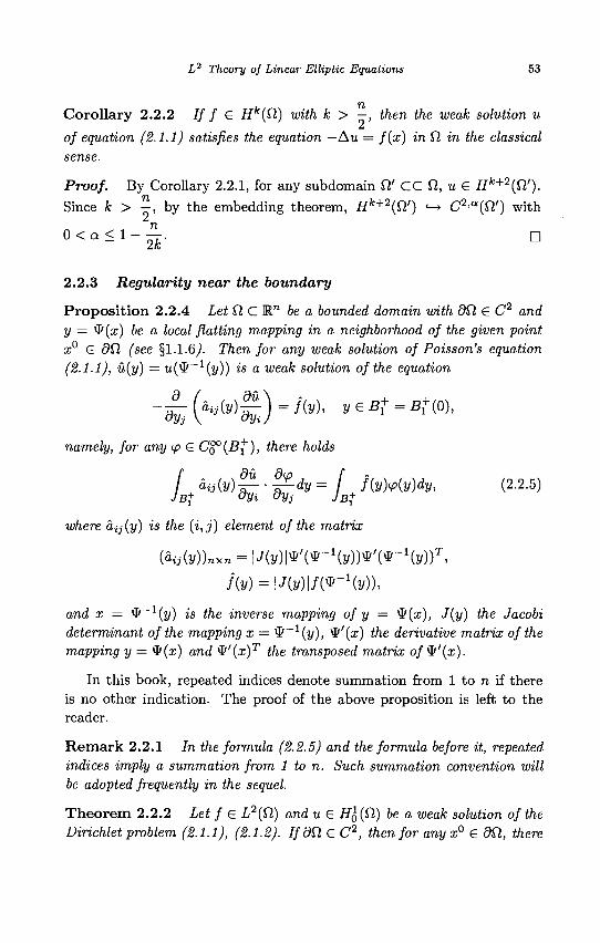
L? Theory of Linear Elliptic Equations 53
Corollary 2.2.2 If f £ Hk(fl) with k > —, then the weak solution u
of equation (2.1.1) satisfies the equation —Au = f(x) in fl in the classical sense.
Proof. By Corollary 2.2.1, for any subdomain Q.' CC Q, u G Hk+2(Q,').
Since k > - , by the embedding theorem, Hk+2{Cl') ^ C2'a(n') with
2.2.3 Regularity near the boundary
Proposi t ion 2.2.4 Let Cl C Rn be a bounded domain with dfl € C2 and y = ty(x) be a local flatting mapping in a neighborhood of the given point x° G dfl (see §1.1.6). Then for any weak solution of Poisson's equation (2.1.1), u(y) —u{^~1(y)) is a weak solution of the equation
namely, for any ip G C^(B^), there holds
[ + ^ l r • j£rdy = i + KvMv)dy, (2-2.5) JB+ °Vi °Vj JB+
where a,ij(y) is the (i,j) element of the matrix
(fiii(y))„xn = | J ( j / ) | * ' (* - 1 (y ) )* ' (* - 1 (y ) ) T ,
f(y) = \J(y)\W-Hy)),
and x = ^ , _ 1(y) is the inverse mapping of y = ^(x), J(y) the Jacobi determinant of the mapping x = * _ 1 ( y ) , W(x) the derivative matrix of the mapping y — $(x) and ^'(x)T the transposed matrix of^'{x).
In this book, repeated indices denote summation from 1 to n if there is no other indication. The proof of the above proposition is left to the reader.
R e m a r k 2.2.1 In the formula (2.2.5) and the formula before it, repeated indices imply a summation from 1 to n. Such summation convention will be adopted frequently in the sequel.
Theorem 2.2.2 Let f G L2(Q) and u G HQ(Q,) be a weak solution of the Dirichlet problem (2.1.1), (2.1.2). IfdCl G C2, then for any x° G dfi, there
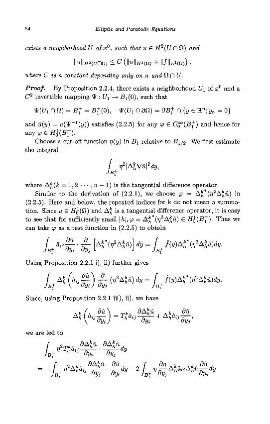
54 Elliptic and Parabolic Equations
exists a neighborhood U of x°, such that u G H2(U n 0) and
IM|jj2(t/nn) < C (\\u\\m{n) + \\fh*(n)),
where C is a constant depending only on n and SlnU.
Proof. By Proposition 2.2.4, there exists a neighborhood U\ of x° and a C2 invertible mapping \P : U\ —> Bi(0), such that
*((7i nfl) = B+ = B+(o), *(t/i n an) = 8B+ n {y e Rn; y„ = 0}
and -t*(y) = u(^!^1(y)) satisfies (2.2.5) for any <p G CQ°(B^) and hence for
any <p G floW)-Choose a cut-off function r](y) in Bi relative to -Bi/2- We first estimate
the integral
JB+ Tj2|A£v«|2dy,
where A£(fc = 1,2, • • • , n — 1) is the tangential difference operator. Similar to the derivation of (2.2.1), we choose <p = A£ (rj2A^u) in
(2.2.5). Here and below, the repeated indices for k do not mean a summation. Since u G HQ(£1) and A£ is a tangential difference operator, it is easy to see that for sufficiently small \h\,<p = A£*(T72A£U) G HQ(B+). Thus we can take tp as a test function in (2.2.5) to obtain
/ ^ 7 P • IT fA£VA^)1 dy = / f(y)tf(r,*Akhu)dy.
Using Proposition 2.2.1 i), ii) further gives
Lt AJ (a« w) w, (,2A!:") * = L t /C'^VAS*)* .
Since, using Proposition 2.2.1 iii), ii), we have
Ah\aijdy-)- h ij~dy~+ ht3dy0'
we are led to
/ .
o„fc. 0AU aA*<2
9Aju 5u / 77
2A^a i j—A- • — d y - 2 / 77—^-A^A^u—<fy
L2 Theory of Linear Elliptic Equations 55
-2f AtaijAkhu^dy+ / /(y)AJtVAJt«)d».
JB{ °Vj °Vi JB{
From this we can proceed similar to the proof of the interior estimate in Theorem 2.2.1 to derive
/ \kkhVu\2dy < C f \Wu\2dy + C f f2dy. (2.2.6)
JB+2 JB+ JB+
To do this, it is to be noted that, since dfl G C2, we have &ij G C1
and hence |A*ciij| < M for some constant M. Another more important fact to be noted is that there exist constants A > 0, ho > 0, such that ThaiMo > AKI2. provided 0 < \h\ < h0.
Using Proposition 2.2.3 ii), from (2.2.6) we see that for any k =
*** G L 2 ( 5 + 2 ) a n d 1,2, •• • ,n — 1 and j = 1,2, •
d2u
dykdyj
•lst/2 dykdyj
dy<C (4 \\7u\2dy + J + f2dy (2.2.7)
Now we rewrite (2.2.5) as
Lt &nnwn • S > = L t
IiyMy)dy - £2n Lt &ij iji • 1 ^
or, after integrating by parts in the second term of the right side,
Li ^nWn • | > = Li {Iiy) + i+ 2n W, ( % ^ ) J *{V)dy-
Prom this and (2.2.7) it follows that ——\ann-r—) G L2(Bt/0). Since it is dyn\ dynJ
l'2' d2u
easy to verify that ann ^ 0 in By2, we further have jr-j G L2(Sjy2) and dy2
L d2u
dVn dy<C \Vu\2dy + C / f'dy.
jBi JBi •L This combined with (2.2.7) implies u(y) G H2(B~f,2). Changing the variable
y to the original one shows that u G H2(U fl fi) with U = }i~1(B^,2) and u satisfies the estimate in Theorem 2.2.2. •
56 Elliptic and Parabolic Equations
Similar to the interior regularity, we also have
Corollary 2.2.3 Let u G HQ (Cl) be a weak solution of the Dirichlet problem (2.1.1), (2.1.2). IfdCl G Ck+2 and f G Hk(Cl) for some nonnegative integer k, then for any x° G dCl, there exists a neighborhood U ofx°, such that u G Hk+2(U n Cl) and
IM|jf*+2(t/nn) < C(H|tfi (fj) + | |/ | | jj*(n)),
where C is a constant depending only on k, n and CinU.
Corollary 2.2.4 If dCl G Ck+2, f G Hk(Cl) and k > | , then for any
x° G dCl, there exists a neighborhood U of x°, such that any weak solution u of the Dirichlet problem (2.1.1), (2.1.2) belongs to C2'a{U C\Cl) with 0 <
Ik
2.2.4 Global regularity
To prove the global regularity of weak solutions, we choose a finite open covering of Cl and decompose the solutions by means of the partition of unity (§1.1.5).
Theorem 2.2.3 Let f G L2(Cl) and u G HQ(CI) be a weak solution of the Dirichlet problem (2.1.1), (2.1.2). If dCl G C2, then u G H2{Cl) and
\HHHO) < C (||«||ffi(n) + ||/||L*(n)) , (2-2.8)
where C is a constant depending only on n and Cl.
Proof. By Theorem 2.2.2, for every x° G dCl, there exists a neighborhood U(x°) such that u G H2(U(x°) n 0) and
\H\H2(U(x°)nu) < C (\H\HHQ) + ll/lk2(n)) •
Using the finite covering theorem we can choose such neighborhoods of N
finite number f/i, • • • , UN to cover dCl. Denote K = Cl \ (J [/*. Then K i=\
is a closed subset of Cl and there exists a subdomain UQ CC Cl, such that U0 D K. Theorem 2.2.1 shows that u G H2(U0), and
NI/r*(c/0) < C (||u||ffi(n) + ||/l|z.3(«)) •
L2 Theory of Linear Elliptic Equations 57
Using the theorem on the partition of unity, we can choose functions
^o, ?7i> • • • i T)N> s uch that
0 < » / i ( x ) < l , V x e K (i = 0,1, - - - ,N), N
» = i
Thus
llullfl"2(n)
N
^ViU i=0
N
<£>• li?2(n) j?2(n) i = 0
< c ( H f f i ( n ) + | | / | |L a ( n ) ) . D
R e m a r k 2.2.2 Under the assumptions of Theorem 2.2.3, we have
hUnn) < C | | / | | L a ( n ) , (2.2.9)
where C is a constant depending only on n and fi.
Proof. We first set <p = u in
/ Vu • Vipdx = J ftpdx, V</> € H^{Q) Jn Jn
and use Cauchy's inequality with e and Poincare's inequality to obtain
/ \Vu\2dx = / fudx Jn Jn
<£- [ u2dx+±- [fdx
1 Jn i£ Jn
<£J± [\Vu\2dx + ± [ fdx, 2 Jn 2e Jn
where fi > 0 is the constant in Poincare's inequality. Choosing e = — then M
gives
/ \Wu\2dx < (j. I fdx. Jn Jn
and further by Poincare's inequality,
/ u2dx <n2 l fdx. Jn Jn
58 Elliptic and Parabolic Equations
Thus the desired inequality (2.2.9) follows by combining the above two estimates and substituting into (2.2.8). •
In the proof of Theorem 2.2.2, the normal derivative of second order is estimated via the equation and the estimates for the tangential derivatives. Repeating this procedure we can estimate higher order derivatives in normal direction.
Theorem 2.2.4 Let u G H&(Q.) be a weak solution of the Dirichlet problem (2.1.1), (2.1.2). Ifdn G Ck+2 and f G Hk{Q) for some nonnegative integer k, then u G Hk+2{Q) and
llulltf*+2(fi) < C (||u||ffi(n) + ||/||ff*(n)),
where C is a constant depending only on k, n and fi.
As an immediate corollary of this theorem, we have
Theorem 2.2.5 Let u G HQ(Q) be a weak solution of the Dirichlet problem (2.1.1), (2.1.2). IfdCl G C°° and f G C°°(Tl), then u G C°°(ty.
Remark 2.2.3 Theorem 2.24 shows that 30, G Ck+2, f G Hk(Cl) imply u £ Hk+2(Q.) and Theorem 2.2.5 shows that <9fi G C°°, f G C°°(Ti) imply u G C°°(f2). This means that the conclusions on the regularity of weak solutions are complete both in Hk(Q) and C°°(fi). In Chapter 8 it will be proved that f G Ca(Q) (a G (0,1)) implies u G C2,a(f2), which means that the conclusion on the regularity of solutions is also complete in Holder spaces. However it is impossible to assert u G C2(0) from f G C(Q).
2.2.5 Study of regularity by means of smoothing operators
Smoothing operators
u£ = JEu= / je(x - y)u(y)dy, (2.2.10) Jo.
instead of difference operators can also be applied to the study of regularity of weak solutions, where js(x) is an arbitrary mollifier. In (2.2.10), u is regarded as zero outside of CI.
It is easy to check the following facts which are an analog of Proposition 2.2.1 i), ii).
Proposition 2.2.5 Let Cl c Mn be a domain.
L2 Theory of Linear Elliptic Equations 59
i) For any u, v £ LJ(fi) vanishing outside ofQ,
/ uevdx = / uv~dx, Jn Jn
where
v~ = J~v= / j~(x - y)u{y)dy, j~(x) = j£(-x).
ii) For any Q' CC fi and sufficiently small e > 0,
DiUe = {DiU)e inQ' (i = 1,2, • • • ,n) .
However we do not have the analog of Proposition 2.2.1 iii) for smoothing operators. This will restrict the application of the present method in the study of regularity.
We also have the following proposition which corresponds to Proposition 2.2.2 and can be proved similarly.
Proposition 2.2.6 Let Q, CM" be a domain and i — 1,2, • • • , n. i)Ifu£ i?1(n) and Q' CC fi, then for sufficiently small e > 0,
\\DiUe\\L2(ni) < | |Diu| |L3(n).
ii) Ifu e if1(fi), fi' CC fi and for sufficiently small e > 0,
||Aw£||L2(fi') < -^
wii/i constant K independent of e, then DiU £ L2(0') and
||Aw||L2(fl') < # •
The proof is left to the reader. We do not state the analog of Proposition 2.2.3, although it does hold. Now we proceed to use smoothing operators to establish the interior
regularity, i.e. to prove Theorem 2.2.1. Choose a cut-off function r)(x) as in the proof of Theorem 2.2.1. By
Proposition 2.2.6 ii), it suffices to establish the estimate
/ Jo.
V2\DiVue\
2dx < C (|M|2„1(n) + | | / | |£ a ( n ) ) (2.2.11)
for some constant C independent of e. Using Proposition 2.2.5 and integrating by parts, we have
/ Jn
rf\DiS7ueYdx n
60 Elliptic and Parabolic Equations
= / A V u e • V(r}2DiUe)dx - 2 / •qDiueVn • A Vuedx Jn Jn
= - / Vu£ • V(A(r?2A«e))da; - 2 / •qDiuEViq • A V u £ d x Jn Jn
= - / Vu- V ( A ( l 2 A M £ ) ) £ " d i - 2 / T]DiU£Wr) • DiVu£dx. Jn Jn
Choosing ip = (Di(r]2DiUe))~ in (2.2.2) and combining the resulting equality with the above formula lead to
/ r)2\DiVue\2dx = - I fiDiirfDiU^-dx - 2 / rjDiUeVri • DiVuedx.
Jn Jn Jn
From this we may deduce (2.2.11) similar to the proof of (2.2.1).
2.3 L2 Theory of General Elliptic Equations
2.3.1 Weak solutions
Now we turn to the following general elliptic equations in divergence form
Lu = -Dj(cnjDiu) + biDiU + cu = f + A / * , (2.3.1)
where ay, 6», c G L°°(fi), / G L2(il), /* G L2(f2), and ay = a^j satisfy the uniform ellipticity condition, i.e. for some constants 0 < A < A,
A|£|2 < a y ( * ) ^ < A|^|2, V£ 6 i n , x € fi.
In this case, we call (2.3.1) uniformly elliptic equations. Here, repeated indices imply a summation from 1 up to n. As in the preceding sections, only the Dirichlet problem with the homogeneous boundary value condition
u = 0 (2.3.2) an
is discussed.
Remark 2.3.1 If a nonhomogeneous boundary value condition
u = g an
is prescribed with g G H1^), then, setting w = u—g, we can change (2.3.1) to an equation for the new unknown function w,
Lw = f + DJi,
L2 Theory of Linear Elliptic Equations 61
where
f = f - hDig - eg, f = f+aijDjg.
The boundary value condition which w satisfies is then a homogeneous one.
If u £ C2(fi) is a solution of equation (2.3.1), then multiplying (2.3.1) with any ip £ CQ?(£1) and integrating over fi lead to, after integrating by parts,
/ (aijDiuDjip + biDiU(p + cwp) dx = (ftp — f%Ditp)dx. (2.3.3) Jn Jn
Conversely, if u £ C2{fl) and for any (p £ CQ°(Q), (2.3.3) holds, then u satisfies (2.3.1) in the classical sense.
Definition 2.3.1 A function u € Hl(Vi) is said to be a weak solution of (2.3.1), if for any ip £ C^(Q), (2.3.3) holds. If, in addition, u £ H^{Cl), then u is said to be a weak solution of (2.3.1), (2.3.2).
2.3.2 Riesz's representation theorem and its application
Riesz's representation theorem applied to Poisson's equation can be carried over to equation (2.3.1) with 6j = 0 (i = 1, • • • , n), i.e. the equation
-DjiaijDiu) +cu = f + Dif*. (2.3.4)
To this purpose, we define a new inner product in HQ(CI) as follows:
(u, v) = / (aijDiuDjV + cuv) dx, Ja
whose corresponding norm is denoted by ||| • |||. It is easy to verify that if c > Co for a certain constant Co, then (•,•) possesses all properties of inner product. For example, using the ellipticity condition and Poincare's inequality, we have, for u £ HQ{Q),
Mil2 = (u, u) = / {aijDiuDjU + cu2) dx Jn
>A / |Vu|2dx + co / u2dx Jn Jn
>a]\u\\2,
62 Elliptic and Parabolic Equations
provided \- c0 > 0, where ||u|| is the norm in #o(Q), M > 0 i s t n e
constant in Poincare's inequality and a = min { - , \- CQ \. From this it I 2 2fi )
follows that (u, u) = 0 implies u = 0. Clearly, for a certain constant /3 > 0,
IIMII2</%II2-Thus
a | | u | | 2 < | |M | | 2 </? | | u | | 2 , (2.3.5)
which implies, in particular, that
F[v] = / (fv - fDiv) dx Jn
is a bounded linear functional in HQ(Q), the same space as H Q ( O ) endowed with the inner product (•, •). Hence, by Riesz's representation theorem (see §2.1.2), there exists a unique u G HQ{£1) such that
(u,v) = / (dijDiuDjV + cuv)dx Jn
= * > ] = f {fv- fDiv) dx, \fv e H&n). Jn
From (2.3.5) we have u £ HQ(Q) and the above formula implies
/ {dijDiuDjtp + cu<p) dx= (ftp - fDitp) dx My e C^(Q), Jn Jn
which means that u is a unique weak solution of (2.3.4), (2.3.2).
Theorem 2.3.1 There exists a constant CQ such that for any f £ L2(Cl), p £ L2(Cl)(i = l,--- ,n), the Dirichlet problem (2.34), (2.3.2) admits a unique weak solution provided c > CQ .
2.3.3 Variational method
Theorem 2.3.1 can also be proved by means of variational method. The functional corresponding to (2.3.4) is
J\v\ = o / (aijDivDjV + cv2) dx- I (fv - fD^) dx. 2 Jn Jn

L2 Theory of Linear Elliptic Equations 63
In fact, arguing as in §2.1.3, we may prove that if u G H^ft) is an extremal of the functional J[v] in HQ(CI), then u is a weak solution of the Dirichlet problem (2.3.4), (2.3.2).
To prove the existence of a minimizer of J[v] in HQ(£1), we first establish the boundedness from below of J[v] in HQ(CI). Using the ellipticity condition and Cauchy's inequality with e, we have
J[v] >7? / \Vv\2dx + ^ / v2dx - | / v2dx 2 Ja 2 Jn 2 JQ
-— f fdx - - f \Vv\2dx - -J- / ffdx. (2.3.6)
This and Poincare's inequality further give
M > i (A_I+ c o _£) j ^ i x _ ^ ^ _ ijf /(/Ml, (a AT)
where /x > 0 is the constant in Poincare's inequality. If Co satisfies —+co >
0, then we may choose e > 0 so small that - ( f- Co — e) > 0. The 2 V /Li /
boundedness from bellow of J\v] in #o (^ ) is thus proved. Combining (2.3.6) with (2.3.7), we obtain
/ v2dx + / \Vv\2dx <Ci+ C2J[v], Vv G H^(il), (2.3.8)
where C\, Ci are constants independent of v G HQ(Q).
Let {ufc} be a minimizing sequence of J[v] in #o(fi). From (2.3.8) it follows that both {uk} and {Vufc} are bounded in L2(Q) and hence there exist a subsequence {MA:I} of {uk} and a function u G i /^ f i ) such that
Ufc, —»• u, Vwfc, —*• Vu in L2(f2) as / —> oo.
In particular, we have
lim / fuk,dx = / fudx, (2.3.9) ; ^°° JQ JO,
lim / fiDiukldx= f fDiudx (i = 1, • •• ,n). (2.3.10)
Moreover, from
/ [a,ijDi(uk, - u)Dj(uk, -u) + c(v,k, - u)2] dx > 0
64 Elliptic and Parabolic Equations
i.e.
/ (cLijDiUktDjUkt +cul)dx Jn
>2 / (aijDiU^DjU + cuk^dx — / (aijDiuDjU + cu2)dx, Jn Ja
it follows that
lim (aijDiiiktDjUkt+cull)dx > (aijDiuDjU +cu2)dx. (2.3.11) i—>oo Jn Jn
Combining (2.3.9), (2.3.10) and (2.3.11),
lim J[uk] = lim J[ufc,] > J[u). k->oo j ^ o o
Thus u is a minimizer of J[v] in #o (fi) an(^ * n e existence of weak solutions of (2.3.4), (2.3.2) is proved.
2.3.4 Lax-Milgram's theorem and its application
It is to be noted that not any elliptic equation of the form (2.3.1) has its corresponding functional so that the variational method can be applied to the Dirichlet problem. If bi (i = 1, • • • ,n) are not all equal to zero, then Riesz's representation theorem also can not be applied. In this case, we need to slightly extend the representation theorem. Lax-Milgram's theorem is one of the very useful results obtained in this direction.
Definition 2.3.2 Let a(u, v) be a bilinear form in the Hilbert space H, i.e. a(u, v) is linear in u and in v respectively.
i) a(u, v) is said to be bounded, if for some constant M > 0,
\a(u,v)\ < M\\u\\\\v\\, Vu,v £ H;
ii) a(u, v) is said to be coercive, if for some constant 8 > 0,
a(u,u)>S\\u\\2, VueH.
Lax-Milgram's Theorem If a(u,v) is a bounded and coercive bilinear form in the Hilbert space H, then for any bounded linear functional F(v) in H, there exists a unique u £ H, such that
F(v)=a(u,v), Vv£H (2.3.12)
L2 Theory of Linear Elliptic Equations 65
and
IMI < ] \ \ n Proof. Since a(u, v) is bilinear and bounded, for any fixed u G H, a(u, •) is a bounded linear functional in H. By Riesz's representation theorem, there exists a unique Au G H, such that
a(u,v) = (Au,v), VveH. (2.3.13)
It is easy to verify from the bilinearity of a(u, v) that the operator A is linear. The boundedness of a(u, v) implies the same property of A:
\\Au\\ < M\\u\\, VuG if.
In addition, since a(u, v) is coercive, we have
S\\u\\2 < a(u,u) = (Au,u) < ||Au||||u||, Vu € H.
Hence
j | |u | | < ||A«||, Vu G H,
which shows the existence of A~l. Now we prove that the range of A, denoted by R(A), is the whole space
H. First of all, R(A) is a closed subset. In fact, if {Auk} C R{A) is a convergent sequence:
lim Auk = v, k~*oo
then, from
S\\UJ - Ufc|| < \\AUJ - Auk\\
we see that {uk} is a Cauchy sequence and hence {uk} is also a convergent sequence:
lim Uk = u. k—too
Hence, by the continuity of the operator A,
lim Auk = Au. fc—»oo
Therefore Au = v, i.e. v G R(A).
66 Elliptic and Parabolic Equations
Suppose R(A) ^ H. Then there exists a nonzero element w e H, such that
(Au, w) = 0 , Vu € H.
In particular, if we choose u = w, then
(Aw,w) = a(w,w) = 0,
which and the coercivity of a(u, v) imply w — 0, a contradiction. Thus R(A) = H.
For any bounded linear functional F(v) in H, by Riesz's representation theorem, there exists a unique w € H, such that \\w\\ = \\F\\ and
F(u) = (w,v), v e H.
Choose u = A~1w. Then
Hl^ll^lllhll^illFH
and
F{v) = {Au,v), veH
which combined with (2.3.13) leads to (2.3.12). •
As an application of Lax-Milgram's theorem, we have
Theorem 2.3.2 There exists a constant CQ, such that for any f € L2(fi) and p € L2(Q.) (i = 1, • • • , n), the Dirichlet problem (2.3.1), (2.3.2) admits a unique weak solution provided c> CQ.
Proof. Denote
a(u,V) = f ( ^ ^ H A ^ + H ^ , V.,, G ^ ( O ) . Jn
Obviously, a(u,v) is bilinear and the boundedness of a,j, bi, c implies the same property of a(u, v):
\a(u,v)\ <C / (|Vu||Vv| + |VM||V| + |u||v|)da; i n
<C(||Vu||La(n)||Vv||La(n) + ||Vu||ia(n)|MU»(n)
+ IMU2(n)IMlL=(n)) <C\\u\\Him\\v\\Hi(Q).
L2 Theory of Linear Elliptic Equations 67
Moreover, using the ellipticity condition and Cauchy's inequality with e, we derive, for u € HQ(Q),
a(u,u) >A| |Vu| | |2 ( n ) -C J |Vu||«|da; + co| |u | |^ ( n )
>A||Vu| | |2 ( n ) - | | | V n | | | 2 ( n ) - 2^||«| |ia(n) +co||«|ll3(n)
c2
Choosing e such that 0 < e < 2A and then taking CQ > ——, it follows that 2s
for some constant S > 0,
a{u,u) > 5\\u\\2Hi{n), Vu € H*(Q),
i.e. a(u, v) is coercive. Now we can apply Lax-Milgram's theorem to the bounded linear func
tional
F(v) = f (fv- fDiv) dx, v e Hi (Q) Ja
to conclude that there exists a unique u € HQ(CI), such that
I M I W < -5\\F\\
and
a(u,v) = F(v), Vu€Hl(£l),
which means that u £ HQ (fl) is the unique weak solution of the Dirichlet problem (2.3.1), (2.3.2). D
2.3.5 Fredholm's alternative theorem and its application
Theorem 2.3.2 merely affirms the weak solvability of the Dirichlet problem (2.3.1), (2.3.2) for the case c > CQ (some constant). To investigate the general case we need the following result (see [Zhong, Fan and Chen (1998)]).
Fredholm's Alternative Theorem Let V be a linear space endowed with a norm, A : V —• V a compact linear operator and I the identity operator. Then there is exact one of the following alternatives:
Elliptic and Parabolic Equations
i) Either the equation
x - Ax = 0 (2.3.14)
has a nontrivial solution x G V; ii) Or the equation
x-Ax = y (2.3.15)
admits a unique solution x G V for any y € V. In other words, if the homogeneous equation (2.3.14) merely has a trivial solution, then the non-homogeneous equation (2.3.15) admits a unique solution for any y G V, or if for some y G V, the solution of the nonhomogeneous equation (2.3.15) is unique, then for any y G V, the nonhomogeneous equation (2.3.15) has a unique solution.
As an immediate application of this theorem, we have
Theorem 2.3.3 There is exact one of the following alternatives: i) Either the boundary value problem
Lu = 0, u
has a nontrivial weak solution; ii) Or the boundary value problem
Lu = f + DJ\ u
= 0 an
= 0 an
has a unique weak solution for any f G L2(il) and p G L2{Q) (i =
!,••• ,n)-
Proof. According to Theorem 2.3.2, there exists a constant vQ, such that the equation
Lu + vu = f + Dif
has a unique weak solution u G HQ(CI) for any / G L2(fi) and /* G L2(f2) (i = 1, • • • ,n) provided v > v0, i.e. the operator L + vl has its inverse (L + vI)~l. Thus
Lu = h = f + Dif
is equivalent to
u = (L + u l ^ h + v{L + J / / ) _ 1 U
L2 Theory of Linear Elliptic Equations 69
or
i.e.
u-v{L + vl)~lu ={L + vl)~lh
u - Au = w,
where A = v(L + i/J)"1, w = (L + vl)~lh G #£(fi). To apply Fredholm's alternative theorem, it suffices to prove the com
pactness of the operator A : HQ(Q) —» HQ(Q). In fact, A can be regarded as a linear operator from l? (fi) to H\ (fi). If we use E to denote the embedding operator from H&(Cl) to L2(fi), then we have A = AE : H%(Sl) -> H&(ft). Since the embedding operator from HQ(SI) to L2(Q) is compact and A is a bounded linear operator as shown in the proof of Theorem 2.3.2, we can assert that the operator A — AE : HQ (fi) —+ HQ (0) is also compact. Thus the conclusion of the theorem follows from Fredholm's alternative theorem.
D
Exercises
1. Introduce the definition of weak solutions of the boundary value problem
' A2u = / , x € 0,
du
dv 0, x G 80,
and prove the existence and uniqueness, where CI C Kn is a bounded domain, / G L2(Cl) and v is the unit normal vector outward to dfl.
2. Define weak solutions of the Neumann problem for Poisson's equation
—Au = / , i e ( ] ,
du
. du 0, x£ dfl,
where Cl C K™ is a bounded domain, / G L2(fl), v is the unit normal vector outward to dfl. And prove that the problem has a weak solution if and only if
/ Jn
f{x)dx = 0.
70 Elliptic and Parabolic Equations
3. Assume A > 0. Define weak solutions of the equation
- A u + Xu = f, i e R "
and prove the existence and uniqueness, where / G L2(Rra). 4. Prove Proposition 2.2.1. 5. Prove Proposition 2.2.4. 6. Let B be the unit ball in Rn and u G HX(B) be a weak solution of
Laplace's equation
- A u = 0, x £ B.
i) Prove u G C°°(B); ii) Prove that if there exists a function v € C°°(M.n) such that u — v G
H^(B), then u G C°°(B). 7. Let u G CQ(IR") be a weak solution of the semi-linear equation
-Au + up = / , xeW1
where / G L2(R"), p > 0. Prove u G iJ2(R"). 8. Establish the theory of regularity for weak solutions of general elliptic
equations.
Chapter 3
L2 Theory of Linear Parabolic Equations
This chapter is a description of the L2 theory of linear parabolic equations parallel to the previous chapter. As in treating elliptic equations, we first discuss a typical equation, i.e. the heat equation in greater detail and then discuss the general linear parabolic equations in divergence form in a brief fashion.
3.1 Energy Method
In this section we introduce the energy method, one of the basic methods available to parabolic equations. Let fl C i " be a bounded domain with smooth boundary dQ, and T > 0 be a constant. Consider the heat equation
— - Au = f{x, t), (x, t)£QT = nx (0, T). (3.1.1)
Different from elliptic equations, we are not permitted to prescribe the condition on the whole boundary of QT- One of the typical conditions to determine the solution is
OPQT
where dpQr is the parabolic boundary of QT, i.e.
dpQT=dQT\(Clx {t = T}).
The problem of finding solutions of equation (3.1.1) satisfying this condition is called the first initial-boundary value problem. For simplicity, we merely
= 0, i.e. the condition d,QT
consider the case g{x, t)
u(x,t)=0, (x,t) edQx (0,T), (3.1.2)
71
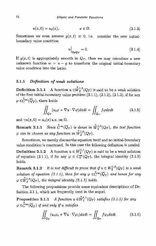
72 Elliptic and Parabolic Equations
u(x,0)=uo(x), xetl. (3.1.3)
Sometimes we even assume g(x,t) = 0, i.e. consider the zero initial-boundary value condition
u = 0 . (3.1.4) opQr
If g(x,t) is appropriately smooth in QT, then we may introduce a new unknown function w = u — g to transform the original initial-boundary value condition into the latter.
3.1.1 Definition of weak solutions
° 11 Definition 3.1.1 A function u £W2 (QT) is said to be a weak solution of the first initial-boundary value problem (3.1.1), (3.1.2), (3.1.3), if for any
<p eC°°(QT), there holds
/ / (ut(p + Vu-Wip)dxdt= fipdxdt (3.1.5) JJQT JJQT
and ju(x, 0) = uo{x) a.e. on Cl. o ° i n
Remark 3.1.1 Since C°°(QT) *S dense in W2 (QT), the test function <p can be chosen as any function in W2 (QT) •
Sometimes, we merely discuss the equation itself and no initial-boundary value condition is concerned. In this case the following definition is needed.
Definition 3.1.2 A function u £ W2' (QT) is said to be a weak solution of equation (3.1.1), if for any tp € CQ°(QT), the integral identity (3.1.5) holds.
Remark 3.1.2 It is not difficult to prove that ifu S W2' (QT) is a weak o
solution of equation (3.1.1), then for any (p &C°°(QT) and hence for any
O . n
tp £W2 (QT), the integral identity (3.1.5) holds.
The following propositions provide some equivalent descriptions of Definition 3.1.1, which are frequently used in the sequel.
° I I Proposition 3.1.1 A function u €W2 ' (QT) satisfies (3.1.5) for any o
<p £C°°(QT) ^ and only tfu satisfies
/ / (uttpt + Vw • Vipt)dxdt = II ftptdxdt (3.1.6) JJQT JJQT
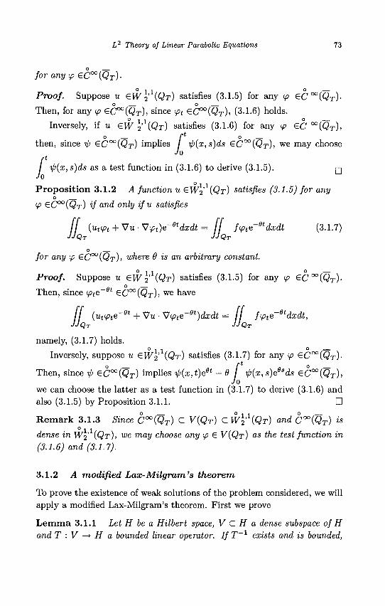
L2 Theory of Linear Parabolic Equations 73
Jo
foranyipeC°°(QT)-
Proof. Suppose u eW^iQr) satisfies (3.1.5) for any ip eC^iQr)-
Then, for any <p eC°°(QT), since <pt eC°°{QT), (3.1.6) holds.
Inversely, if u GW 1A(QT) satisfies (3.1.6) for any ip £C °°(QT)> o _ /"* o _
then, since tp &C°°(QT) implies / ip(x,s)ds &C°°(QT), w e may choose
Jo
ip(x,s)ds as a test function in (3.1.6) to derive (3.1.5). rj 0 I 1 Proposition 3.1.2 A function u GWJ (QT) satisfies (3.1.5) for any
o
<p &C°°(QT) if and only tfu satisfies
if (uttpt + Vu-V<pt)e-etdxdt= [[ fipte~9tdxdt (3.1.7) JJQT JJQT
o
for any <p GC°°(<3x)> where 6 is an arbitrary constant.
Proof. Suppose u &WI'1(QT) satisfies (3.1.5) for any <p eC^iQr)-
Then, since y>te~et &C°°(QT)I
w e have
/ / (ut(pte'et + Vu • S/<pte-et)dxdt = / / f<pte-etdxdt, JJQT JJQT
namely, (3.1.7) holds. o . , o
Inversely, suppose u £W2 ' (QT) satisfies (3.1.7) for any (p eC°°(Qr)-ft
Then, since ip GC°°(QT) implies ip(x,t)eet -6 ip(x,s)eesds GC°°(QT), Jo
we can choose the latter as a test function in (3.1.7) to derive (3.1.6) and also (3.1.5) by Proposition 3.1.1. •
Remark 3.1.3 Since C°°(QT) C V{QT) CW\'1(QT) and C°°(QT) is ° I I
dense in W2 (QT), we may choose any <p> € V(QT) as the test function in (3.1.6) and (3.1.7).
3.1.2 A modified Lax-Milgram's theorem
To prove the existence of weak solutions of the problem considered, we will apply a modified Lax-Milgram's theorem. First we prove
Lemma 3.1.1 Let H be a Hilbert space, V C H a dense subspace of H and T : V —> H a bounded linear operator. If T _ 1 exists and is bounded,
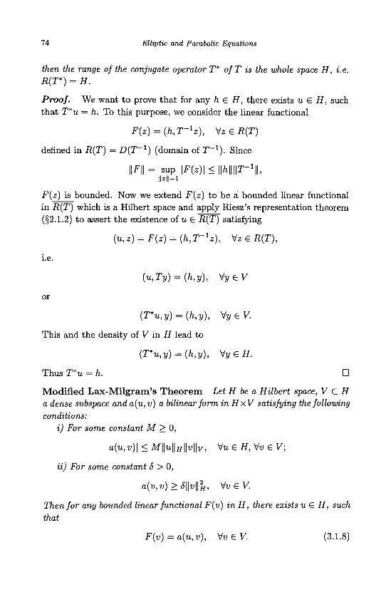
74 Elliptic and Parabolic Equations
then the range of the conjugate operator T* of T is the whole space H, i. e. R(T*) = H.
Proof. We want to prove that for any h € H, there exists u € H, such that T*u = h. To this purpose, we consider the linear functional
F(z) = (h,T~1z), Vz£R(T)
defined in R(T) = D{T~l) (domain of T~l). Since
| |F| | = sup \F(z)\ < \\h\\\\T-% IMI=i
F(z) is bounded. Now we extend F(z) to be a bounded linear functional in R(T) which is a Hilbert space and apply Riesz's representation theorem (§2.1.2) to assert the existence of u S R(T) satisfying
(u,z) = F(z) = (h,T-1z), VzER(T),
i.e.
(u,Ty) = (h,y), VyeV
or
(T*u,y) = (h,y), VyeV.
This and the density of V in H lead to
(T*u,y) = (h,y), Vy£H.
Thus T*u = h. U
Modified Lax-Milgram's Theorem Let H be a Hilbert space, V C H a dense subspace and a(u, v) a bilinear form in HxV satisfying the following conditions:
i) For some constant M > 0,
|o(u,w)| < M||u||ff||i;||v, Vu £H,\/v£ V;
ii) For some constant S > 0,
a(v,v)>6\\vfH, V«GV.
Then for any bounded linear functional F(v) in H, there exists u G H, such that
F(v)=a(u,v), W e F . (3.1.8)
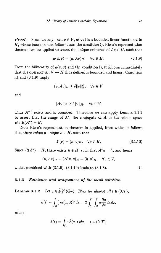
L2 Theory of Linear Parabolic Equations 75
Proof. Since for any fixed v £ V, a(-,v) is a bounded linear functional in H, whose boundedness follows from the condition i), Riesz's representation theorem can be applied to assert the unique existence of Av G H, such that
a(u,v) = (u,Av)H, Mu&H. (3.1.9)
Prom the bilinearity of a(u,v) and the condition i), it follows immediately that the operator A : V —• H thus denned is bounded and linear. Condition ii) and (3.1.9) imply
(v,Av)H>S\\v\\2H, VveV
and
\\Av\\H>S\\v\\H, VueV.
Thus A~l exists and is bounded. Therefore we can apply Lemma 3.1.1 to assert that the range of A*, the conjugate of A, is the whole space H : R{A*) = H.
Now Riesz's representation theorem is applied, from which it follows that there exists a unique h £ H, such that
F(v) = (h,v)H, VveH. (3.1.10)
Since R(A*) = H, there exists u G H, such that A*u — h, and hence
(«, Av)H = (A*u, v)H = (h, v)H, VU G V,
which combined with (3.1.9), (3.1.10) leads to (3.1.8). •
3.1.3 Existence and uniqueness of the weak solution
Lemma 3.1.2 Let u ew\'1 {QT). Then for almost all t G (0,T),
h(t) - I (lu(x,Q)))2dx = 2 / / u-^dxds, Ja Jo Jo. dt
where
h(t) = / u2(x,t)dx, t<= (0,T). Ja
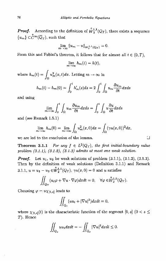
76 Elliptic and Parabolic Equations
1 1 Proof. According to the definition of W2' (QT), there exists a sequence
{um} CC°°(QT), such that
m l i m J | u m - u | | ^ 1 , 1 ( ^ = 0 .
Prom this and Fubini's theorem, it follows that for almost all t € (0,T),
lim hm(t) = h(t), m—MX)
where hm(t) = / u2n(x,t)dx. Letting m —> oo in
Jn ft ft /» Q
hm(t) - hm(0) = / h'm(s)ds = 2 / / um—^dxds
and using
lim / / Um—^p-dxds = u—dxds ™^°°Jo Jn °t J0 Jn dt
and (see Remark 1.5.1)
lim hm(0) = lim / uL(x,0)dx = / {~iu(x,0))2dx, m ^ o o m->oo Jn Jn
we are led to the conclusion of the lemma. •
Theorem 3.1.1 For any f € L2(QT), the first initial-boundary value problem (3.1.1), (3.1.2), (3.1.3) admits at most one weak solution.
Proof. Let u\, un. be weak solutions of problem (3.1.1), (3.1.2), (3.1.3). Then by the definition of weak solutions (Definition 3.1.1) and Remark
0 i i 3.1.1, u = u\ — ui €W2 ' (QT), JU(X, 0) = 0 and u satisfies
/ / (utip + Vu • Vip)dxdt = 0, V</> &W12°{QT)-JJQT
Choosing <p — u\[o,s] leads to
/ / (uut JJQ,
+ \Vu\2)dxdt = 0, iQs
where X[o,s](t) is the characteristic function of the segment [0, s] (0 < s < T). Hence
/ / uutdxdt = - \Wu\2dxdt < 0.
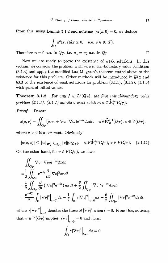
L2 Theory of Linear Parabolic Equations 77
From this, using Lemma 3.1.2 and noticing ju(x, 0) = 0, we deduce
/ u2(x, s)dx < 0, a.e. s € (0, T). Jn
Therefore u = 0 a.e. in QT, i.e. ui = u<i a.e. in QT- • Now we are ready to prove the existence of weak solutions. In this
section, we consider the problem with zero initial-boundary value condition (3.1.4) and apply the modified Lax-Milgram's theorem stated above to the existence for this problem. Other methods will be introduced in §3.2 and §3.3 to the existence of weak solutions for problem (3.1.1), (3.1.2), (3.1.3) with general initial values.
Theorem 3.1.2 For any f £ L2(QT), the first initial-boundary value * i i
problem (3.1.1), (3.1.4) admits a weak solution u £W2 (QT)-
Proof. Denote
a(u, v) = / / [utvt + Vu • Vvt)e-etdxdt, u £WI'X(QT), V £ V(QT), JJQT
where 0 > 0 is a constant. Obviously
Hu,v)\ < \\U\\WI,I{QT)\\V\\V{QT), U ew^iQT), v e V(QT). (3.1.11)
On the other hand, for v G V(QT), we have
/ / Vv • Vvte-etdxdt
=\IL«-et>v?dxdt
= \ j l ^t(\Vv\2e-et)dxdt+9-JJ \W\h-°*dxdt IQ
-6T f IVd2 dx-- f 7 | V d 2 dx + - [f \Vv\2e~etdxdt,
Jn t=T 2 Jn t=o 2 JJQT
where7|Vv| t=o
denotes the trace of | Vu|2 when t = 0. Prom this, noticing
that v € V(QT) implies -yS/v 0 and hence t=o
Jn dx = 0,
it=o
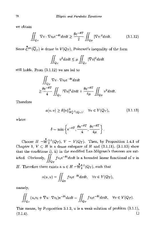
78 Elliptic and Parabolic Equations
we obtain
-8T / / Vv • S7vte-etdxdt > ——- / / \Vv\2dxdt. (3.1.12)
JJQT 2 JJQT
• Since C°°(QT) is dense in V(QT), Poincare's inequality of the form
/ / v2dxdt < fi / / \Vv\2dxdt JJQT JJQT IQT JJQT
still holds. From (3.1.12) we are led to
/ / Vi> • Vvte~etdxdt JjQT
-6T rr Qa-8T
Therefore
where
Qp-vT rr flp-^ rr
a(v,v)>S\\v\\2wi,1{QT), VveV(QT), (3.1.13)
5 = min < eT 9e~eT ee~eT
6 ' 4 ' 4/i
Choose # =wl'\QT), V = V(QT)- Then, by Proposition 1.4.1 of Chapter 1, V C H is a dense subspace of # and (3.1.11), (3.1.13) show that the conditions i), ii) in the modified Lax-Milgram's theorem are sat
isfied. Obviously, / / fvte etdxdt is a bounded linear functional of v in JJQT
* 1 1
H. Therefore there exists a u G H =Wi (QT), such that
IQT
namely,
a(u,v)= [f fvte-9tdxdt, ^v£V{QT), JJQT
ff (utvt + Vu-Vvt)Q-6tdxdt= ff fvte-etdxdt, Vv G V(Qr). JJQT JJQT
This means, by Proposition 3.1.2, u is a weak solution of problem (3.1.1), (3.1.4). •
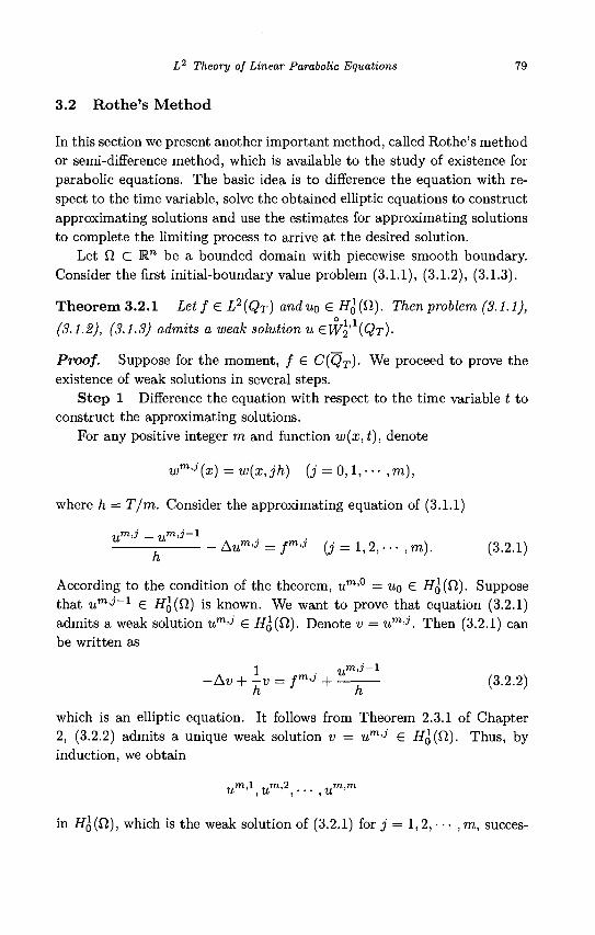
L2 Theory of Linear Parabolic Equations 79
3.2 Rothe's Method
In this section we present another important method, called Rothe's method or semi-difference method, which is available to the study of existence for parabolic equations. The basic idea is to difference the equation with respect to the time variable, solve the obtained elliptic equations to construct approximating solutions and use the estimates for approximating solutions to complete the limiting process to arrive at the desired solution.
Let Q C M.n be a bounded domain with piecewise smooth boundary. Consider the first initial-boundary value problem (3.1.1), (3.1.2), (3.1.3).
Theorem 3.2.1 Let f G L2(QT) anduQ G # o ( n ) - Then problem (3.1.1),
(3.1.2), (3.1.3) admits a weak solution u GWy (QT)-
Proof. Suppose for the moment, / G C(QT). We proceed to prove the existence of weak solutions in several steps.
Step 1 Difference the equation with respect to the time variable t to construct the approximating solutions.
For any positive integer m and function w(x,t), denote
wm'j(x)=w{x,jh) (j = 0,l,--- ,m),
where h = T/m. Consider the approximating equation of (3.1.1)
Aum,3=fm,: {j = lj2,...,m). (3.2.1)
According to the condition of the theorem, um'° = UQ G HQ(Q). Suppose that um '-J -1 G HQ(Q) is known. We want to prove that equation (3.2.1) admits a weak solution u m j G HQ(Q). Denote v = u m j . Then (3.2.1) can be written as
1 vm,j-l -Av + TV = fm<3 + — T — (3.2.2)
which is an elliptic equation. It follows from Theorem 2.3.1 of Chapter 2, (3.2.2) admits a unique weak solution v = u m j G HQ(Q,). Thus, by induction, we obtain
um'\um'2,--- ,um'm
in HQ(Q), which is the weak solution of (3.2.1) for j = 1,2, • • • ,m, succes-
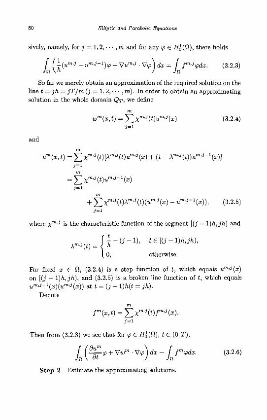
80 Elliptic and Parabolic Equations
sively, namely, for j = 1,2, • • • , m and for any ip £ HQ(£1), there holds
/ {^^ ~ "m'^1)^ + Wum,i " V < ^) dx = / /m 'Vz- (3.2.3)
So far we merely obtain an approximation of the required solution on the line t = jh = jT/m (j = 1,2, • • • , m). In order to obtain an approximating solution in the whole domain QT, we define
m
wm{x,t) =Y,Xm'j(t)um'j(x) (3.2.4)
and
« m ( i , t )=5] f J ' ( t )P ( t ) i ' , " J W + (1 - AmJ(t))uroj'-1(i)]
= 5>mj'(*K,J'-1(*) m
+ 53xm,j i(*)A" , J(t)(«T, , , , '(x) - u r o J - 1 ( x ) ) , (3-2-5)
where xm 'J ' is the characteristic function of the segment [(j — l)h,jh) and
A m J ( 4 ) = n - o - - D , *€[(,--i)M/o, ( 0, otherwise.
For fixed x e Cl, (3.2.4) is a step function of t, which equals um'*{x) on [{j — l)h,jh), and (3.2.5) is a broken line function of t, which equals umJ-l{x){um>i{x)) at t = {j- l)h(t = jh).
Denote
771
fm(x,t) = j2xm'jwm,jw-
Then from (3.2.3) we see that for ip € H&(Q,), t € (0,T),
j (^-<p + Vwm • V</> j dr = /" /"Vdar. (3.2.6)
S tep 2 Estimate the approximating solutions.
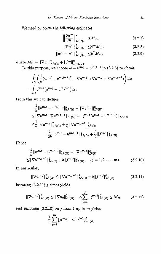
I? Theory of Linear Parabolic Equations
We need to prove the following estimates
dum 2
81
dt LHQT) <Mm,
\\^m\\h(QT) <4TMm,
\\™m-um\\lHQT)<h2Mm,
where Mm = ||Vuo||£a(n) + ll/mll!2(QT). To this purpose, we choose ip — u m j — u m , J _ 1 in (3.2.3) to obtain
= / fm'j{um>i -um'j-l)dx.
Prom this we can deduce
(3.2.7)
(3.2.8)
(3.2.9)
))dx
i . | | „ m J _ •> , m J- 1 | l 2 4- \\\7n,m<3\\'i
h\\u u llL2(n) + l l V u \\L
L2(Q)
• _l l . , in, j .,m,j —1||2 I " II fm,}\\2
2h" "L'W + 2"* " L 2
lli,2(n)
h 21 (")•
Hence
^ l l u u llL2(n) + l l V u llL2(fi)
< l |V Um ^ - 1 | | ! 2 ( n ) + / i | | / ^ | | i 2 ( n ) , (j = l , 2 , . . . ,m).
In particular,
iiv«mj'iiia(n) < i i v t ^ - 1 ! ^ + h\\rm*{ay
Iterating (3.2.11) j times yields
l |V«m J | |£ a ( n ) < | |V«o| | ia ( n ) + / i ^ | | / m ' i | | 2 ( n ) < M m
and summing (3.2.10) on j from 1 up to m yields
1 m 1 V II n
(3.2.10)
(3.2.11)
(3.2.12)
| i m , j _ u m , j - l | | 2
J = l L2(Q.)
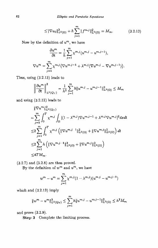
82 Elliptic and Parabolic Equations
<l|V«o||£a(n) + * £ \\fm'j\\lHci) = Mm.
Now by the definition of um, we have
dun_ ~ ~ ~h.
(3.2.13)
dt
- m
Vum = Y^Xm,j(^tJ-m'j'1 + Am,J'(Vum,J' - Vum j ' - 1)) .
Thus, using (3.2.13) leads to
dun
dt
Z •. Til
LHQT) n j = l
and using (3.2.12) leads to
HVum|||2(QT) m pT
= J2 Xm,j / 1(1 - An,J ')V«mj ' -1 + \m'jVum'j\2dxdt •=1 Jo Jn
< 2 E / *m'j (llV«m-,'-1|lia(n) + HVu r o ' i i2 ( n )) dt j = l 0
m
^ J X I I V I ^ - 1 ! ! ^ ) + ||VumJ||ia(n))
<4TMm.
(3.2.7) and (3.2.8) are then proved. By the definition of wm and um, we have
^ X m , i ( l - Am'J')(um'J' - um>j~l)
which and (3.2.13) imply
and prove (3.2.9). Step 3 Complete the limiting process.
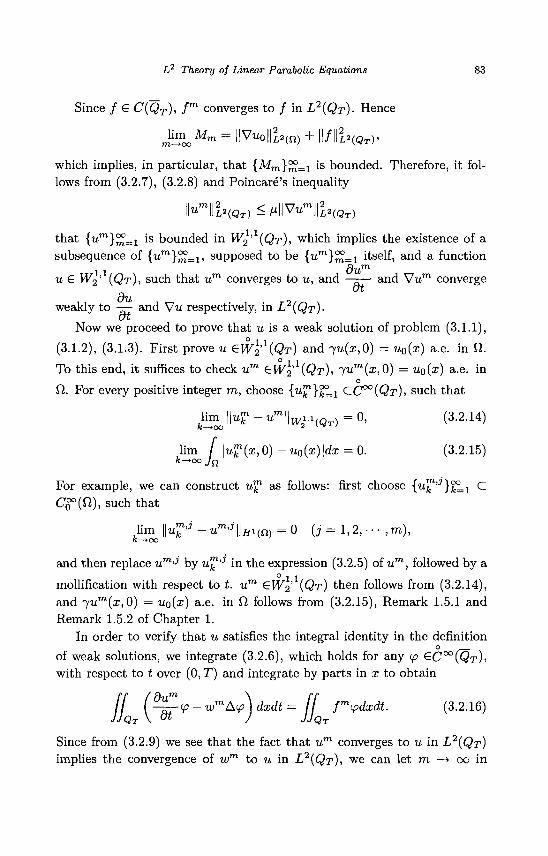
L2 Theory of Linear Parabolic Equations 83
Since / £ C(QT), fm converges to / in L2(QT)- Hence
Jirn^M™ = ||V«o||£a{n) + | | / | | £ 2 W T ) ,
which implies, in particular, that {Mm}m=i is bounded. Therefore, it follows from (3.2.7), (3.2.8) and Poincare's inequality
•u m l l 2 <? n l l V 7 i / m l l 2
that {um}^=1 is bounded in W2' (QT), which implies the existence of a subsequence of { u m } ~ = 1 , supposed to be {um}^=1 itself, and a function
u £ W2' (QT), such that um converges to u, and —-— and Vu m converge
dii weakly to — and Vu respectively, in L2(QT)-
(JTI
Now we proceed to prove that u is a weak solution of problem (3.1.1),
(3.1.2), (3.1.3). First prove u £W\'1(QT) and -yu(x,0) = u0(x) a.e. in £2. ° 1 1
To this end, it suffices to check um £Wy (Qr)> ryurn(x)0) = UQ{X) a.e. in o
fl. For every positive integer m, choose {u^}(^L1 C C ° ° ( Q T ) , such that limJuZ-um\\wui(QT)=0, (3.2.14)
lim / \uf(x,0) -uo(x)\dx = 0. (3.2.15)
For example, we can construct u™ as follows: first choose {u™'3}'%L1 C C§°(Cl), such that
lim \\u™'j - umJ\\^m = 0 (j = 1,2, • • • ,m), K—>00
and then replace u m J by u™'-1 in the expression (3.2.5) of um, followed by a ° I I mollification with respect to t. um SWV (QT) then follows from (3.2.14),
and 'yum(x, 0) = UQ(X) a.e. in Cl follows from (3.2.15), Remark 1.5.1 and Remark 1.5.2 of Chapter 1.
In order to verify that u satisfies the integral identity in the definition o
of weak solutions, we integrate (3.2.6), which holds for any <p GC°°(QT),
with respect to t over (0, T) and integrate by parts in x to obtain
jf ('^<p-wmA<p\dxdt= jf fmipdxdt. (3.2.16)
Since from (3.2.9) we see that the fact that um converges to u in L2(QT)
implies the convergence of wm to u in L2(QT), we can let m —> oo in
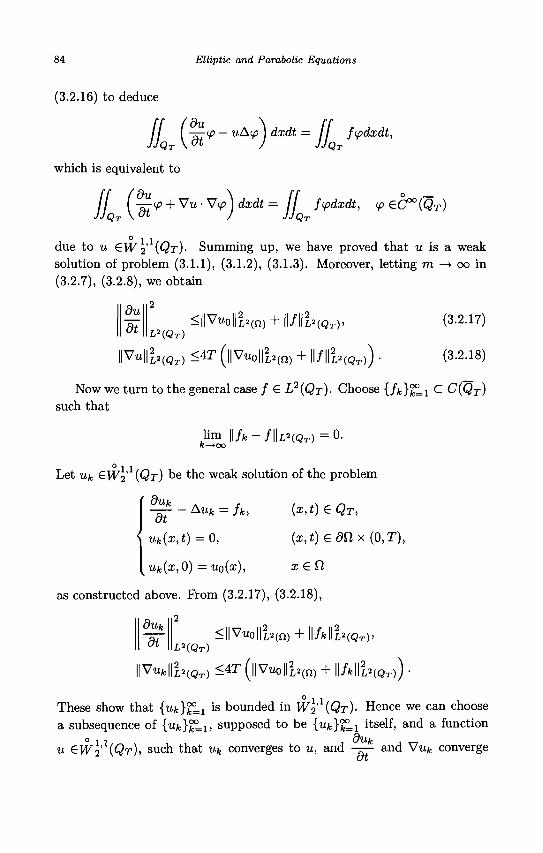
84 Elliptic and Parabolic Equations
(3.2.16) to deduce
/ / ( "PT^ ~ U^(P ) dxdt = II ftpdxdt,
which is equivalent to
' du
JJQ. dt tp + Vu • Vip I dxdt
JJQ-ftpdxdt, <p eC°°(Q r )
° 1 1 due to u £W2 (QT)- Summing up, we have proved that u is a weak solution of problem (3.1.1), (3.1.2), (3.1.3). Moreover, letting m —> oo in (3.2.7), (3.2.8), we obtain
du <l|V«o||£a(n) + ll/lli 'W T),
L2(QT)
HV«||£aWr) <4T (||V«o||ia(n) + ll/|lia(QT))
(3.2.17)
(3.2.18)
Now we turn to the general case / S L2(QT)- Choose {fk}^! C C(QT) such that
lim || fk - f\\L*(QT) = 0.
fc—>oo
0 1 1
Let uk GW2 (QT) be the weak solution of the problem ( duk
dt
uk(x,t) = 0,
Aufc = fk, (x,t)eQT,
(x,t)e9Slx (0,T),
[uk(x,0) = u0(x), xeQ,
as constructed above. Prom (3.2.17), (3.2.18),
duk
dt <HVuo||£a(n) + I IAIIL»W T) . LHQT)
l|V«fc||ia(Qr) <4T (||Vu0|||2(n) + \\fk\\lHQT)) -
0 1 1 These show that {wfc}^i is bounded in W2' (QT)- Hence we can choose
a subsequence of {ufc}£Li, supposed to be {uk}^ itself, and a function
u GWl'X(Qr), such that uk converges to u, and -^— and Vuk converge
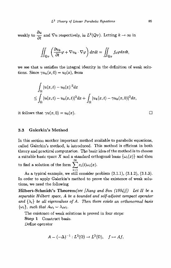
L2 Theory of Linear Parabolic Equations 85
weakly to — and Vu respectively, in L2(QT)- Letting k —> oo in
/ / l-zrlP + 'Vuk-'V(p)dxdt= fkipdxdt,
we see that u satisfies the integral identity in the definition of weak solutions. Since 7Ufc(:r,0) = uo(x), from
/ \u(x,t) — uo(x)\2dx Jfi
< / \u(x,i) - uk(x,t)\2dx + / \uk(x,t) -juk(x, 0)\2dx, Jn Jn
it follows that ju(x, 0) = UQ(X). O
3.3 Galerkin's Method
In this section another important method available to parabolic equations, called Galerkin's method, is introduced. This method is efficient in both theory and practical computation. The basic idea of the method is to choose a suitable basic space X and a standard orthogonal basis {u>i(x)} and then
oo
to find a solution of the form Yjcj(i)a;i(x). i = l
As a typical example, we still consider problem (3.1.1), (3.1.2), (3.1.3). In order to apply Galerkin's method to prove the existence of weak solutions, we need the following Hilbert-Schmidt's Theoremfsee [Jiang and Sun (1994)]) Let H be a separable Hilbert space, A be a bounded and self-adjoint compact operator and {Aj} be all eigenvalues of A. Then there exists an orthonormal basis {WJ}, such that Auii = AjWj.
The existence of weak solutions is proved in four steps: Step 1 Construct basis. Define operator
A = ( - A ) " 1 : L2(n) - L2(Q), f -> Af,
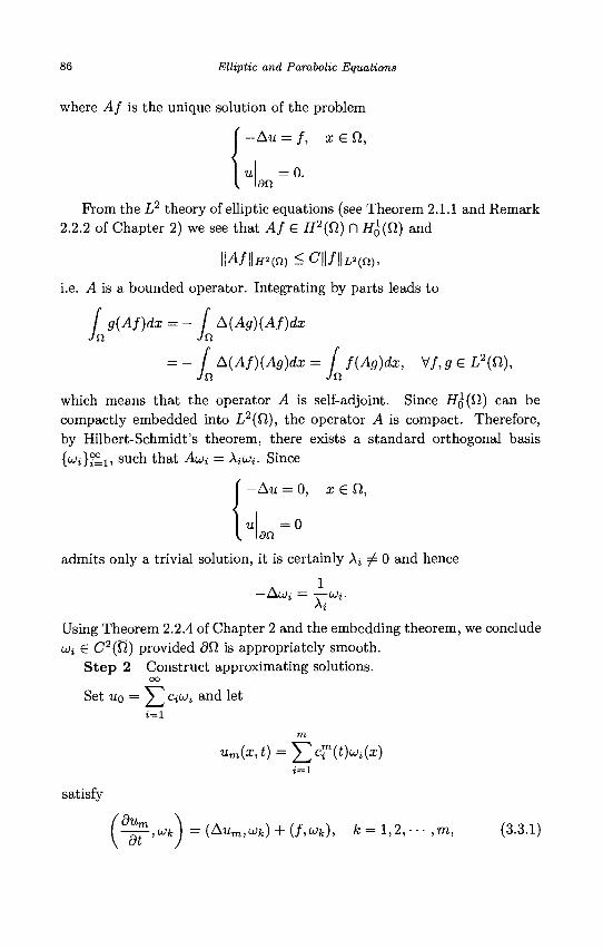
86 Elliptic and Parabolic Equations
J JQ
where Af is the unique solution of the problem
—Au — / , x £ ( l ,
= 0. an
From the L2 theory of elliptic equations (see Theorem 2.1.1 and Remark 2.2.2 of Chapter 2) we see that Af e H2(Q.) D #o(fi) and
\\Af\\HHQ) < C\\f\\LHn),
i.e. A is a bounded operator. Integrating by parts leads to
/ g(Af)dx = - [ A(Ag)(Af)dx JQ JQ
= - [ A(Af)(Ag)dx = f f(Ag)dx, Vf,g £ L2(ft), JQ JQ
which means that the operator A is self-adjoint. Since HQ(£1) can be compactly embedded into L2(£l), the operator A is compact. Therefore, by Hilbert-Schmidt's theorem, there exists a standard orthogonal basis {ui}iZi, such that AuJi = AjWj. Since
Au = o, x € n,
= 0 dQ
admits only a trivial solution, it is certainly \%^Q and hence
- A u > j = -— w». Aj
Using Theorem 2.2.4 of Chapter 2 and the embedding theorem, we conclude Wj € C2(fi) provided dd is appropriately smooth.
S tep 2 Construct approximating solutions.
i = l
Set t*o = / ^ QWi and let
m
satisfy
'dUjn
, dt u>k ) = (Aum,LJk) + {f,uk), k = 1,2, ••• ,m, (3.3.1)
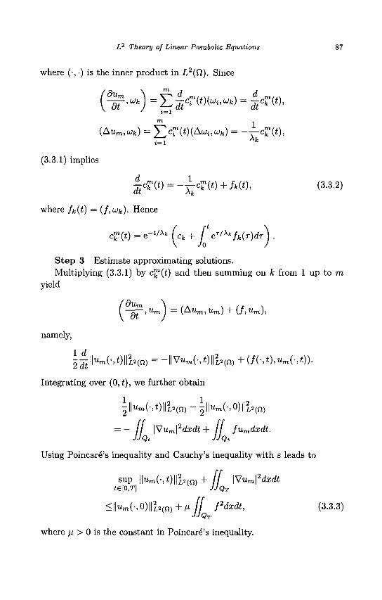
L2 Theory of Linear Parabolic Equations 87
where (•, •) is the inner product in L2(Q). Since
x ' i=\ m 1
(Aum,wfe) = ^c™(t)(Awi,u f e) = ——cjp(i),
(3.3.1) implies
±cT(t) = -j-cT(t)+fk(t), (3.3.2)
where fk(t) = (/.wjt)- Hence
# ( * ) = e-*/A* f cfc + y e^x"fk(r)dA .
Step 3 Estimate approximating solutions. Multiplying (3.3.1) by c™(£) and then summing on k from 1 up to m
yield
namely,
2^llum(-,i)ll |2(n) = -||V«m(-,t)lli,a(n) + (/(-»*).«m(-.*))-
Integrating over (0,£), we further obtain
2ll«i"(-.*)llia(n) - 2llu'"( -'0)lli2(n)
= — II \Vum\2dxdt+ / / fumdxdt. JJQt JJQt
Using Poincaxe's inequality and Cauchy's inequality with e leads to
sup | |w m ( - , i ) | | | 2 ( n ) + / / \Vum\2dxdt te[0,T] JJQT
<hm(-M\h{a)+^JJ fdxdt, (3.3.3)
where fi > 0 is the constant in Poincaxe's inequality.
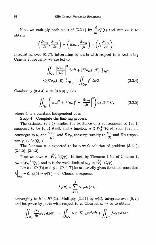
88 Elliptic and Parabolic Equations
Next we multiply both sides of (3.3.1) by —c™(£) and sum on k to
obtain
dum dum\ ( dum\ ( dun
-dr'-dr) = {Aum>-dr) + {f>-d-t Integrating over (0, T), integrating by parts with respect to x and using Cauchy's inequality we are led to
\dum
dt jf Jf^\ dxdt+\\Vum(;T)\\lHn)
<l |V«m(- ,0) | | i a ( n )+ / / fdxdt. (3.3.4) JJQT IQ
Combining (3.3.4) with (3.3.3) yields
2
I |Um|2 + |Vum |2 + QT \
du, m dt
dxdt < C, (3.3.5)
where C is a constant independent of m. S tep 4 Complete the limiting process. The estimate (3.3.5) implies the existence of a subsequence of {um},
supposed to be {um} itself, and a function u S W2' {QT), such that um , dum , _ , , du , _
converges to u, and —-— and \um converge weakly to -— and vu respec-at at
tively, in L2(QT)-
The function u is expected to be a weak solution of problem (3.1.1), (3.1.2), (3.1.3).
0 1 1
First we have u £W<2 {QT)- In fact, by Theorem 1.5.4 of Chapter 1, O i i O i i
um GW2' (QT) and u is the weak limit of um in Wi (QT)-
Let h S C2(Q) and ip e C2[0, T] be arbitrarily given functions such that
h = 0 , ip(0) = tp(T) = 0. Choose a sequence
3 hj(x) = '^2ajkUk(x),
fe=l
converging to h in H1^). Multiply (3.3.1) by ip(i), integrate over (0,T) and integrate by parts with respect to x. Then let m —-> oo to obtain
/ / —Ukipdxdt = - Vu • Vu)ki>dxdt + / / fuikiidxdt.
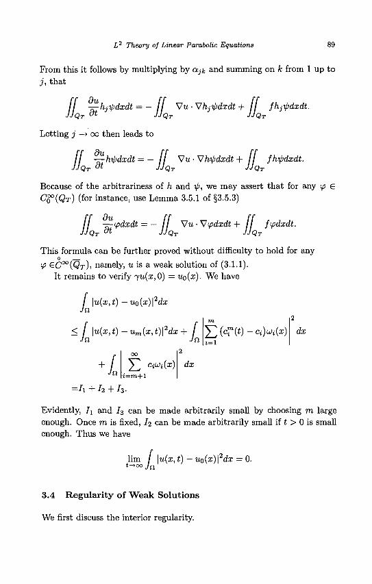
L2 Theory of Linear Parabolic Equations 89
Prom this it follows by multiplying by ajk and summing on k from 1 up to j , that
JJQ-
du hjtpdxdt -II
JJQT
Vu • Vhjipdxdt + / / fhjipdxdt II JJQT
Letting j —> co then leads to
du
JJQi dt hipdxdt
JJQ-Vu-Vhipdxdt+ / / f hipdxdt.
JJQT
Because of the arbitrariness of h and ip, we may assert that for any ip £ C O ° ( O T ) (for instance, use Lemma 3.5.1 of §3.5.3)
/ / —<pdxdt = - / / Vu • Wipdxdt + / / fipdxdt. JJQT ™ JJQT JJQT
This formula can be further proved without difficulty to hold for any o
<p €C°° (<9T) I namely, u is a weak solution of (3.1.1). It remains to verify 7u(:r,0) = UQ(X). We have
/ \u(x,t) — uo(x)\2dx Ja
; / \u(x,t) - um(x,t)\2dx + I Ja. Ja
£(c?(t)-*)<*(*) i = l
dx
+ J Jn
^2 CiU)i(x) l=7Tl + l
dx
=h + h + h
Evidently, I\ and I3 can be made arbitrarily small by choosing m large enough. Once m is fixed, Ii can be made arbitrarily small if t > 0 is small enough. Thus we have
lim / \u(x,t) — uo(x)\2dx = 0.
3.4 Regularity of Weak Solutions
We first discuss the interior regularity.
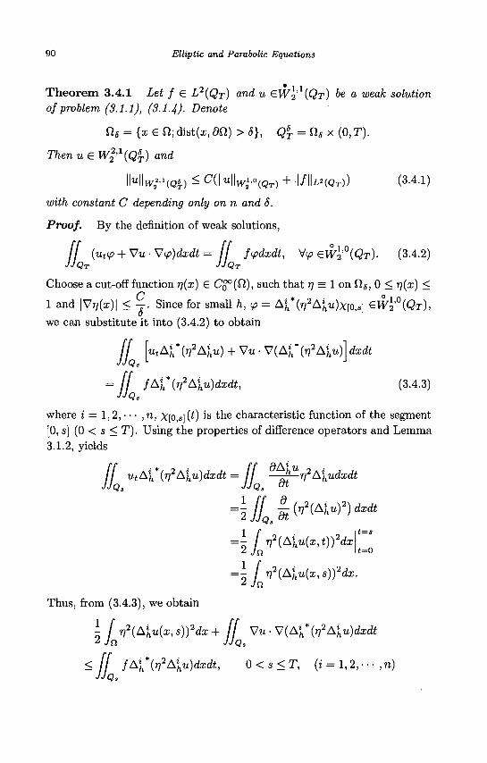
90 Elliptic and Parabolic Equations
Theorem 3.4.1 Let f € L2(QT) and u €W\X{QT) be a weak solution of problem (3.1.1), (3.14). Denote
fls = {xe Q; dist(x, 9fi) > 6}, Q5T = Slsx (0,T).
Thenu£Wl'l{QsT) and
\M\WI\QI.) < <?(Hlv^'°(QT) + ll/ll^(QT)) (3.4.1)
with constant C depending only on n and 5.
Proof. By the definition of weak solutions,
/ / (ut<p + Vu • Vtp)dxdt = if fipdxdt, V<p ewl'°(QT)- (3.4.2) JJQT JJQT
Choose a cut-off function r)(x) £ 0^(0.), such that rj = 1 on fig, 0 < rj{x) <
1 and |V77(ar)| < —. Since for small h, tp = A{*(r]2Aiu)x[o,s} €WI'°(QT),
we can substitute it into (3.4.2) to obtain
ff L A ^ V A > ) + Vu • V(Aj / (v2Aiu)} dxdt JJQs L J
= ff fAi*(r,2A{u)dxdt, (3.4.3) JJQs
where i = 1,2, • • • , n, X[o,s](t) is the characteristic function of the segment [0, s] (0 < s < T). Using the properties of difference operators and Lemma 3.1.2, yields
JJ utAih\n
2Aihu)dxdt=JJ ^^r,2Aiudxdt
-\j]Q}t^^hu)2)dxdt
= 1 f r,2(Aiu(x,t))2dxt=S
* Jn t=o
=\ f V2(Aiu(x,s))2dx.
J it
Thus, from (3.4.3), we obtain
\ f n2{Aihu{x,s))2dx+ ff Vu.V(Ai*(r,2Aiu)dxdt
z Jn JJQ3
< ff fA\*{r]2Aiu)dxdt, 0 < s < T, (i = 1,2, • • • , n)
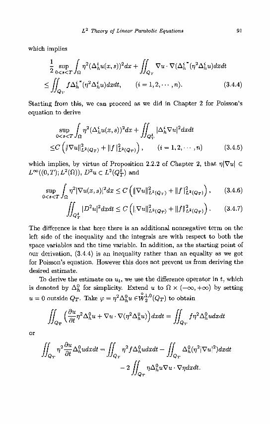
L2 Theory of Linear Parabolic Equations 91
which implies
i sup f rj2{Aihu{x,s))2dx + ff Vu-V(Ai*(r)2Aiu)dxdt
2o<s<r7n JJQT
< ff fA^^A^dxdt, (i = l , 2 , - . - , n ) . (3.4.4) JJQT
Starting from this, we can proceed as we did in Chapter 2 for Poisson's equation to derive
sup / rj2(Aihu{x,s))2dx + ff \A]yu\2dxdt
0<s<TJa JJQ%.
< c ( | | V U | | i 2 ( Q T ) + | | / | | i 2 ( Q T ) ) , (t = l , 2 , - . . , n ) (3.4.5)
which implies, by virtue of Proposition 2.2.2 of Chapter 2, that r?|Vu| S L°°((0,T);L2(f2)), D2u € L2(Q5
T) and
sup / r,2\Vu(x, s)\2dx < C ( | |V«| | i a ( Q T ) + | | / | | i 2 ( Q T ) ) , (3.4.6) o<s<TJn K '
ff \D2u\2dxdt < C ( | |V«| | i a ( Q T ) + | | / | | | 2 ( Q T ) ) • (3.4.7) JJQT
The difference is that here there is an additional nonnegative term on the left side of the inequality and the integrals are with respect to both the space variables and the time variable. In addition, as the starting point of our derivation, (3.4.4) is an inequality rather than an equality as we got for Poisson's equation. However this does not prevent us from deriving the desired estimate.
To derive the estimate on Ut, we use the difference operator in t, which is denoted by A° for simplicity. Extend u to Q x (-co, +oo) by setting
u = 0 outside QT- Take tp = r]2A°hu €WI'°(QT) to obtain
jf (^rj1Alu + Vu-V{r}2A°hu))dxdt = ff fV
2A°hudxdt
or
/ / rj2^A°hudxdt = ff r)2fA°hudxdt- ff A°h{r)2\Vu\2)dxdt JJQT &t JJQT JJQT
- 2 / / r)A°huVu • Vrjdxdt. JJQT
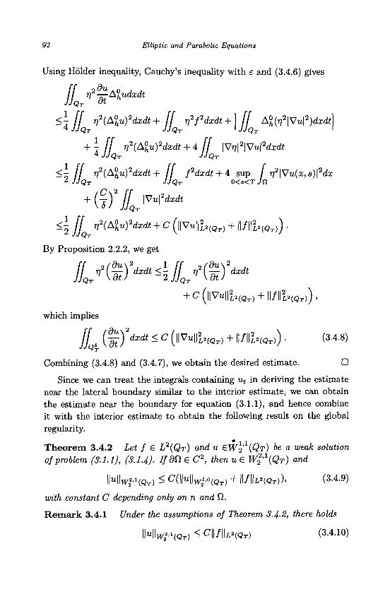
92 Elliptic and Parabolic Equations
Using Holder inequality, Cauchy's inequality with e and (3.4.6) gives
r]2—A0hudxdt
QT dt I
<- (I rj2(A°hu)2dxdt+ [f rffdxdt + l [[ A°h(r)2\Vu\2)dxdt 4 JJQT JJQT ' JJQT
+ \ fl r)2(A°hu)2dxdt + 4 / / |Vr/|2|Vu|2dxrft 4 JJQT JJQT
<\ II r]2(A°hu)2dxdt+ f[ fdxdt + 4 sup f r}2\Vu(x,s)\2dx * JJQT JJQT O<S<T Ja
+ ( T ) 7 1 | V * | 2 < M
< i If •r,HK")2dxdt + C (ll V«||l,(„r i + VHIHOT)) • >QT
By Proposition 2.2.2, we get
//a/(t)«4//0/(§^ + C( | |VU| | 2
L 2 ( Q T ) + | | / | | | 2 ( Q T ) ) ,
which implies
JJ s (^fdxdt < C (||VU\\2LHQT) + \\f\\lHQT)) . (3.4.8)
Combining (3.4.8) and (3.4.7), we obtain the desired estimate. •
Since we can treat the integrals containing ut in deriving the estimate near the lateral boundary similar to the interior estimate, we can obtain the estimate near the boundary for equation (3.1.1), and hence combine it with the interior estimate to obtain the following result on the global regularity.
Theorem 3.4.2 Let f £ L2(QT) and u €W\'X{QT) be a weak solution of problem (3.1.1), (3.14). If dQ e C2, then u £ Wl'l{QT) and
H I V ^ W T ) < C{\\U\\W1,O{QT) + | | / | | L ' W T ) ) , (3A9)
with constant C depending only on n and fi.
Remark 3.4.1 Under the assumptions of Theorem 3.4-2, there holds
\\u\\w^(QT)<C\\f\\L2{QT) (3.4.10)
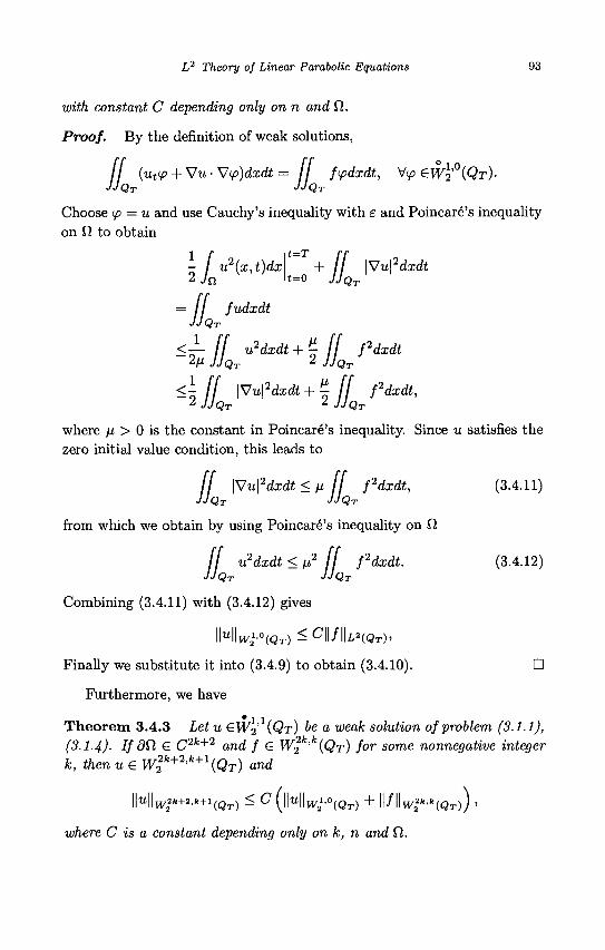
L2 Theory of Linear Parabolic Equations 93
with constant C depending only on n and Q..
Proof. By the definition of weak solutions,
ff (uttp + Vu-Vtp)dxdt= / / ftpdxdt, V<p ewl'°(QT)• JJQT JJQT
Choose (p = u and use Cauchy's inequality with e and Poincare's inequality on fi to obtain
- / u2(x,t)dx + / / \Vu\2dxdt 2jn «=o JJQT
= / / fudxdt JJQT
<— ff u2dxdt + £ ff fdxdt 2/u JJQT 2 JJQT
<\ ff \Vu\2dxdt+^ ff fdxdt, 2 JJQT 2 JJQT IQT * JJQi
where \x > 0 is the constant in Poincare's inequality. Since u satisfies the zero initial value condition, this leads to
ff \Vu\2dxdt < fi ff fdxdt, (3.4.11) JJQT JJQT
from which we obtain by using Poincare's inequality on D.
ff u2dxdt < \x2 ff fdxdt. (3.4.12) JJQT JJQT
Combining (3.4.11) with (3.4.12) gives
Finally we substitute it into (3.4.9) to obtain (3.4.10). •
Furthermore, we have
* I I T h e o r e m 3.4.3 Let u GW2 (QT) be a weak solution of problem (3.1.1),
(3.14). If dQ, e C2k+2 and f € W22fe,fe(Qr) for some nonnegative integer
k, then u e W2k+2'k+1 (QT) and
\\u\\wik+2,k+nQT) < C ( | | t i | | W a i . o W T ) + \\f\\w^k(QT)) >
where C is a constant depending only on k, n and Q,.
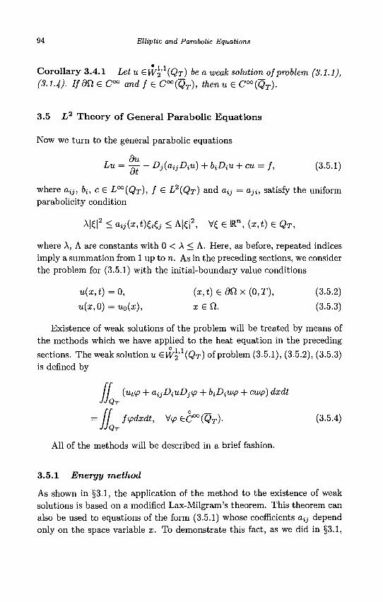
94 Elliptic and Parabolic Equations
Corollary 3.4.1 Let u &W\'1{QT) be a weak solution of problem (3.1.1), (3.1.4). IfdSl G C°° and f G C°°(QT), then u G C°°(QT).
3.5 L2 Theory of General Parabolic Equations
Now we turn to the general parabolic equations
Lu— — - Dj(aijDiu) + biDiU + cu = f, (3.5.1)
where ay, bt, c G Lco(QT), f G L2{QT) and oy = aji, satisfy the uniform parabolicity condition
A|£|2 < dijix^Uj < A|^|2, V£ € Rn , (x,t) G QT,
where A, A are constants with 0 < A < A. Here, as before, repeated indices imply a summation from 1 up to n. As in the preceding sections, we consider the problem for (3.5.1) with the initial-boundary value conditions
u(x,t) = 0,
u(x,0) = u0(x),
( x , t ) 6 3 f ix (0,T),
l £ f l .
(3.5.2)
(3.5.3)
Existence of weak solutions of the problem will be treated by means of the methods which we have applied to the heat equation in the preceding sections. The weak solution u GW2' (QT) of problem (3.5.1), (3.5.2), (3.5.3) is defined by
I {ut<p + aijDiuDjip + biDiwp + cwp) dxdt QT
ftpdxdt, V</> GC°°(QT). (3.5.4) QT
All of the methods will be described in a brief fashion.
3.5.1 Energy method
As shown in §3.1, the application of the method to the existence of weak solutions is based on a modified Lax-Milgram's theorem. This theorem can also be used to equations of the form (3.5.1) whose coefficients ay depend only on the space variable x. To demonstrate this fact, as we did in §3.1,
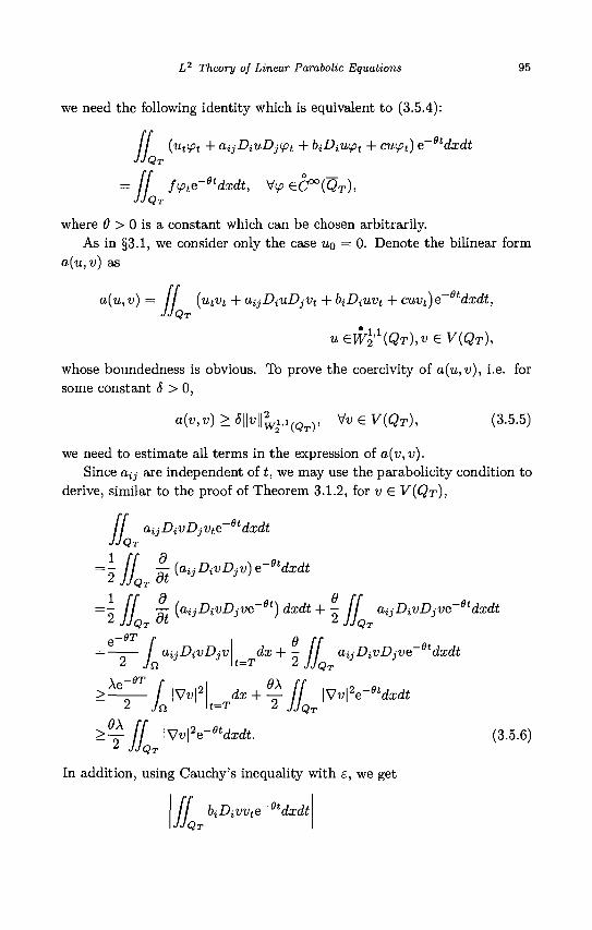
L2 Theory of Linear Parabolic Equations 95
we need the following identity which is equivalent to (3.5.4):
/ / (utft + aijDiuDjifit + biDiU(pt + cu<pt) e~etdxdt
II fipte-etdxdt, V^eC°°(Qr) ,
where 8 > 0 is a constant which can be chosen arbitrarily. As in §3.1, we consider only the case UQ = 0. Denote the bilinear form
a(u, v) as
a(u, v) = / / (utvt + UijDiuDjVt + biDiUvt + cuvt)e~~etdxdt, JJQT
UQW\'1{QT),V£V{QT),
whose boundedness is obvious. To prove the coercivity of a(u, v), i.e. for some constant S > 0,
a(v,v) > % | | ^ I . I W T ) , VveV(QT), (3.5.5)
we need to estimate all terms in the expression of a(v, v). Since a^ are independent of t, we may use the parabohcity condition to
derive, similar to the proof of Theorem 3.1.2, for v € V(QT),
11 a,ijDivDjVte~~0tdxdt JJQT
= 2 / / ^-(aijDivDjv)e~etdxdt
=x / / TT (aaDivDiVe"61) dxdt + - aaDivDiVe~etdxdt 2 JJQT dt K > 2 JJQT
I auDivDjV dx + - / / aaDivDiVe~etdxdt Jn t=r 2JJQT
IQT
-8T
2
Ae- e T
f \Vv Jo.
dx + t=T
2e~0tdxdt.
°4 II \Vv\2e~etdxdt 2 JJQT
(3.5.6)
In addition, using Cauchy's inequality with e, we get
/ / biDiVvte~6tdxdt JJQT
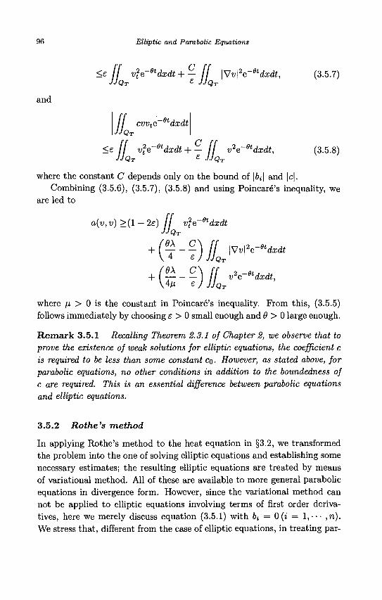
96 Elliptic and Parabolic Equations
<e ff v2e~etdxdt +- ff \Wv\2e~8tdxdt, (3.5.7)
and
/ / cvvte~8tdxdt\ JJQT I
<e / / v?e-0tdxdt + - ff v2e~etdxdt, (3.5.8) JJQT £ JJQT
where the constant C depends only on the bound of \bi\ and \c\. Combining (3.5.6), (3.5.7), (3.5.8) and using Poincare's inequality, we
are led to
a(v,v) >(1 - 2e) / / v2e~etdxdt JJQT
+ (e-±-C) ff \Vv\2e-0tdxdt 4 e , JJQT
+ IS-?)1"V"^ where /x > 0 is the constant in Poincare's inequality. From this, (3.5.5) follows immediately by choosing e > 0 small enough and 6 > 0 large enough.
Remark 3.5.1 Recalling Theorem 2.3.1 of Chapter 2, we observe that to prove the existence of weak solutions for elliptic equations, the coefficient c is required to be less than some constant CQ. However, as stated above, for parabolic equations, no other conditions in addition to the boundedness of c are required. This is an essential difference between parabolic equations and elliptic equations.
3.5.2 Rothe's method
In applying Rothe's method to the heat equation in §3.2, we transformed the problem into the one of solving elliptic equations and establishing some necessary estimates; the resulting elliptic equations are treated by means of variational method. All of these are available to more general parabolic equations in divergence form. However, since the variational method can not be applied to elliptic equations involving terms of first order derivatives, here we merely discuss equation (3.5.1) with bt = 0(i = 1,- • • ,n) . We stress that, different from the case of elliptic equations, in treating par-
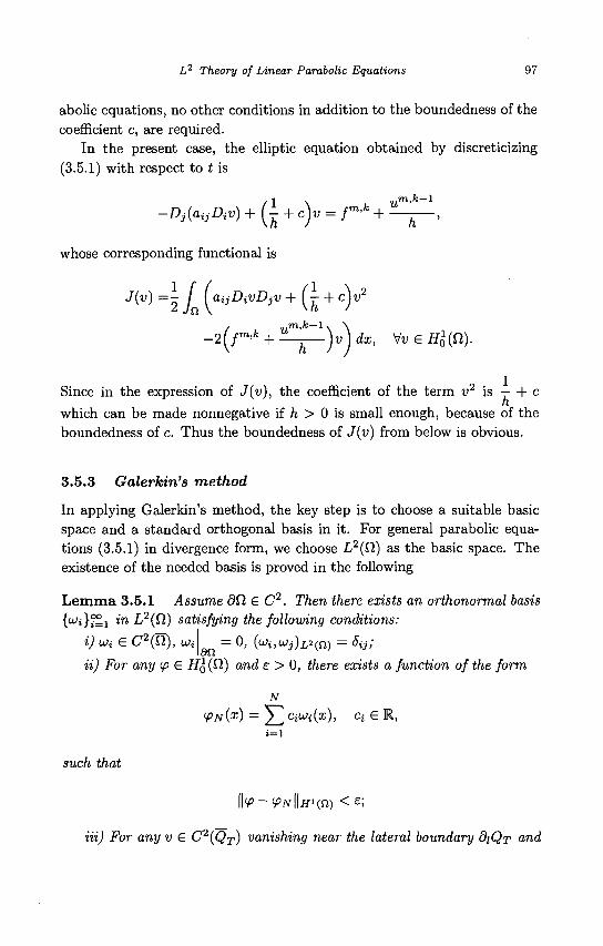
L2 Theory of Linear Parabolic Equations 97
abolic equations, no other conditions in addition to the boundedness of the coefficient c, are required.
In the present case, the elliptic equation obtained by discreticizing (3.5.1) with respect to t is
,,m,k-l j . + c)v = fm'k + ——,
whose corresponding functional is
J{v) = - / (aijDivDjV +[r+ cjv2
. , .m,fc- lN \
-2(/m' ,s + ^ — y)dx, Wei^O) .
Since in the expression of J(v), the coefficient of the term v2 is — + c h
which can be made nonnegative if h > 0 is small enough, because of the boundedness of c. Thus the boundedness of J(v) from below is obvious.
3.5.3 Galerkin's method
In applying Galerkin's method, the key step is to choose a suitable basic space and a standard orthogonal basis in it. For general parabolic equations (3.5.1) in divergence form, we choose L2(Q) as the basic space. The existence of the needed basis is proved in the following
Lemma 3.5.1 Assume 80, 6 C2. Then there exists an orthonormal basis
(wi}iSi in L2(Q) satisfying the following conditions:
i) ua e C2(f2), Ui = 0, (ui,Wj)Li(n) = <5y; oil
it) For any ip £ HQ (Q.) and e > 0, there exists a function of the form
N
<PN(X) = 'Y^ciu:i(x), cteR, i= l
such that
\\V~<PN\\H^Q) < £ ;
Hi) For any v € C2(QT) vanishing near the lateral boundary DIQT and
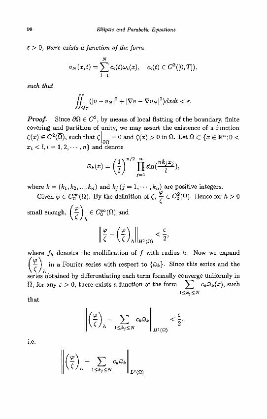
98 Elliptic and Parabolic Equations
e > 0, there exists a function of the form
N
vN(x,t) = Y,Ci{t)^i{x), a(t) G C2([0,T]), i = l
such that
/ / (\v-vN\2+ \Vv-VvN\2)dxdt <e. JJQT IQT
Proof. Since dCl € C2 , by means of local flatting of the boundary, finite
covering and partition of unity, we may assert the existence of a function
C(x) G C2(f2), such that C = 0 and C(x) > 0 in fi. Let Q, C {x G Rn; 0 <
^ < Z, i = 1,2, • • • , n} and denote
Wfc(a;)
n/2 n
nSin(
where A; = (fci, fc2,..., fcn) and fcj (j = 1, • • • , fcn) are positive integers.
Given ip G Cg°(fi). By the definition of C, j G C$(fi). Hence for h > 0
small enough, ( ^ ) G Cg°(ft) and
<P _ (<P <
#!(") 2'
where /^ denotes the mollification of / with radius h. Now we expand
I — I in a Fourier series with respect to {u)fc}. Since this series and the
series obtained by differentiating each term formally converge uniformly in Q, for any e > 0, there exists a function of the form VJ Ck<*>k{x), such
l<kj<N
that
(7) - E c^ v s / ' » l<kj<N
£
< 2 ' if!(fi)
i.e.
f £ CfcWfe
>» l<kj<N L2(fi)
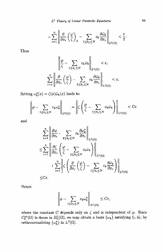
L2 Theory of Linear Parabolic Equations
+E dXi\<Jh !<!" <N
< L2(Cl)
Thus
<P E l<kj<N
CkUJk < £ ,
E 9 /V
L2(f2)
cfcDfc a^vcy ^ * * * <e.
L 2 ( f i )
Setting wj(x) = ((x)wfc(:E) leads to
l<kj<N L2(Q)
M 7 ~ E CkGlk <Ce L 2 ( f i )
and
£ i = l
n
sE i=\
dw v-^ 9^t
^ i<tr<N ^ L2(n)
- ^ 7 - y " cfcwfe
M ^ 1<7?<N L2(n)
+E » = i
c d ftp
dxt \ C 5Z c* Kki<N
duk dxi
i-si&j L2(n) <Ce.
Hence
V? - 5 Z CkU}*k l<kj<N
<Ce,
m(n)
where the constant C depends only on C and is independent of <p. Since C^°(fi) is dense in HQ(Q,), we may obtain a basis {wfc} satisfying i), ii), by orthonormalizing {w£} in L2(fi).
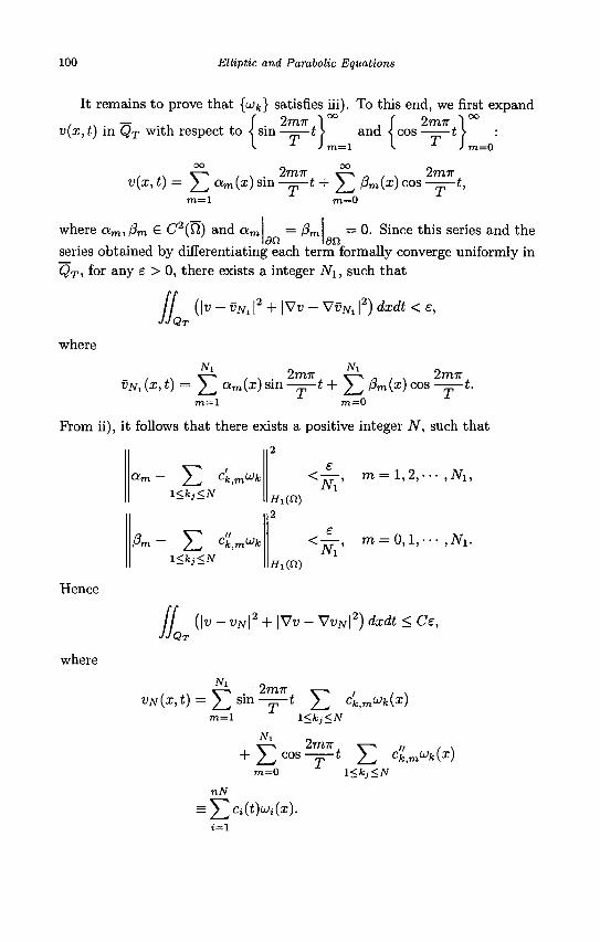
100 Elliptic and Parabolic Equations
It remains to prove that {uJk} satisfies iii). To this end, we first expand / \ . T=T . i i . 2rrm
v(x, t) in QT with respect to ^ sin t | s , „ — <) m = _ and ( c o s _ , | ^ :
, ,. v-^ / N . 2m7r y-^ . , . 2m-K v(x, t) = Z-, am{X) Sin —^-t + 2 ^ Pm(x) COS - ^ - * ,
m = l m=0
= /?m = 0. Since this series and the an Ian
series obtained by differentiating each term formally converge uniformly in
where am,/3m € C2(fi) and a„
series obtained by differentiatii QT, for any e > 0, there exists a integer Ni, such that
/ / (\v - vNl |2 + |Vu - VvNl |2) ctecft < e,
where
/ \ V"» / \ • 2m7T ^ r — > . . . 2m7T vNl (x, t) = 2 ^ am(aO sin -—-* + 2 ^ ftn(i) cos —jT*-
m=l m—0
Prom ii), it follows that there exists a positive integer N, such that
am- Yl c'k,mUk i<fcj<w
cfc,mwfc l<fcj<JV
Hi(n) 2
< — , m = 0, l , --- ,iVi.
tfi(n)
Hence
where
/ / {\v-vN\2 + \Vv-VvN\2)dxdt<Ce, JJQT
NI
VN 2TO7T
(x, t) = 2^ sin - — t 2_, V ^ l 1 ) m = l l<kj<N
Ni
c o s — - t 2 ^ Ck.mWkW m=0 \<kj<N
nN
•:^2ci(t)Wi(x). i= l
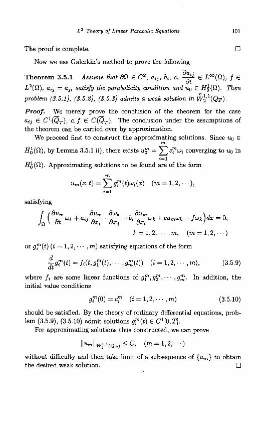
L2 Theory of Linear Parabolic Equations 101
The proof is complete. •
Now we use Galerkin's method to prove the following
Theorem 3.5.1 Assume that dCl G C2, o y , bt, c, -^- G L°°(fi), / G
L2(0), a,ij = aji satisfy the parabolicity condition and UQ G HQ(Q). Then ° I I
problem (3.5.1), (3.5.2), (3.5.3) admits a weak solution in WY (QT)-
Proof. We merely prove the conclusion of the theorem for the case atj G Cl{QT), c,f£ C(QT). The conclusion under the assumptions of the theorem can be carried over by approximation.
We proceed first to construct the approximating solutions. Since UQ G m
HQ(£1), by Lemma 3.5.1 ii), there exists u™ — ^ J c ™ ^ converging to UQ in i=i
Ho(fi). Approximating solutions to be found are of the form
m
um{x, t) = Y2 9T(t)ui(x) (m = 1,2, • • •), i=l
satisfying
(dum dum duik , , dum , ^ , n [~ariJl<: + aii~d~ ' ~Q~. + bi~Q~UJk + ^rn^k ~ J^kjdx = 0,
fc = 1 ,2 , •• • , m , ( m = l , 2 , • • • )
or g™(t) (i = 1,2, • • • , m) satisfying equations of the form
jt9r(t)=fi(t,9T(t),---,9Z(t)) (t = l > 2 , - . - , m ) , (3.5.9)
where fa are some linear functions of g™,g™, • • • ,g^- I*1 addition, the initial value conditions
9T(0)=c? (» = l ,2 > - . - > m) (3.5.10)
should be satisfied. By the theory of ordinary differential equations, problem (3.5.9), (3.5.10) admit solutions $"(*) G C^O.T].
For approximating solutions thus constructed, we can prove
\\um\\w^{QT)<C, (m = l ,2,---)
without difficulty and then take limit of a subsequence of {um} to obtain the desired weak solution. D
/
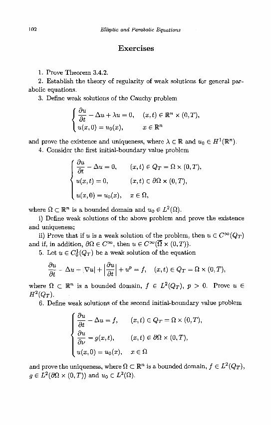
102 Elliptic and Parabolic Equations
Exercises
1. Prove Theorem 3.4.2. 2. Establish the theory of regularity of weak solutions for general par
abolic equations. 3. Define weak solutions of the Cauchy problem
du — -Au + Xu = 0, (x,t) e l " x (0,T), Oil
u(x,0) = u0(x), x £
and prove the existence and uniqueness, where A g R and UQ £ H 1(R"). 4. Consider the first initial-boundary value problem
du
u{x,t) = 0,
- A u = 0, ( i , f ) 6 Q r = fix(0,r),
(x,t)edQx (0,T),
u(x,0) = u0(x), xeQ.,
where O c Rn is a bounded domain and u0 £ L2(Q,). i) Define weak solutions of the above problem and prove the existence
and uniqueness; ii) Prove that if u is a weak solution of the problem, then u £ C°°(QT)
and if, in addition, dQ £ C°°, then u £ C°°(Ti x (0, T)). 5. Let u £ CQ(QT) be a weak solution of the equation
du Hi - Au + IVul +
du
at + up = f, fat) G QT = SI x (0,T),
where fi c Rn is a bounded domain, / £ L2(QT), p > 0. Prove u £
H2(QT). 6. Define weak solutions of the second initial-boundary value problem
r du dt
-Au = f, (i,t)GQr = nx(0,T),
du (x,t) e f f l x (0,T),
•u(x,0) = u0(x), x &Q,
and prove the uniqueness, where 0 C R™ is a bounded domain, / € L2(QT), g e L2{dCl x (0,T)) and u0 £ L2(^) .
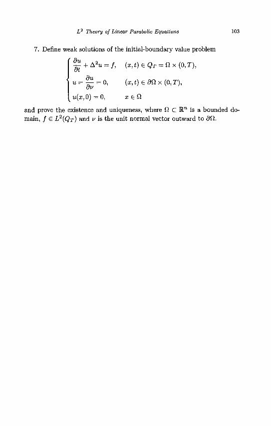
L2 Theory of Linear Parabolic Equations 103
7. Define weak solutions of the initial-boundary value problem
' du — + A2u = f, ( i , t ) e O r = n x ( 0 , r ) ,
du u = — =0,
ov u(x,0) = 0,
(x,t)£dQx (0,T),
and prove the existence and uniqueness, where fl c Rn is a bounded domain, / G L2(QT) and v is the unit normal vector outward to 80..

Chapter 4
De Giorgi Iteration and Moser Iteration
This chapter is devoted to a discussion of properties of weak solutions. Two powerful techniques, the De Giorgi iteration and the Moser iteration, are introduced, which can be applied not only to linear elliptic and parabolic equations in divergence form, but also to quasilinear equations, not only to the estimate of maximum norm, but also to the study of other properties, such as regularity of weak solutions. In order to expose the basic idea and main points of these techniques in a limited space, we confine ourselves basically to Poisson's equation and the heat equation, and apply the techniques merely to the estimate of maximum norm of weak solutions.
4.1 Global Boundedness Estimates of Weak Solutions of Poisson's Equation
In this section we illustrate the De Giorgi iteration by applying it to the estimate of maximum norm of weak solutions for Poisson's equation.
4.1.1 Weak maximum principle for solutions of Laplace's equation
Definition 4.1.1 Let u G Hl{1H). The least upper bound and the greatest lower bound of u on 0, and dQ, are defined as
supu = inf{/; (u — /)+ = 0, a.e. in Q,},
supu = inf {7; (u — l)+ S HQ(Q)}, dU
inf u = — sup(—u), inf u = — sup(—u), n n an a n
105
106 Elliptic and Parabolic Equations
where s+ = max{s,0}.
In case u is continuous on Q, the definition of supu, inf u and supu, n n an
inf u coincides with the usual one. For sup u and inf u, this is obvious and an (f n for sup u and inf u, this follows from the discussion of the trace of functions
a n 9Q.
in Hl(Sl) (see §1.5). Let Cl c M.n be a bounded domain. Consider Laplace's equation
- A u = 0, xeCl. (4.1.1)
Proposition 4.1.1 Let u e iJx(fi) be a weak solution of Laplace's equation (4.1.1). Then
supu < supu. n an
Proof. By the definition of weak solutions, u satisfies
Vu-V<pdx = 0 (4.1.2) / JQ
/ Jo.
for any tp £ CQ°(Q) and hence for any ip € HQ(Q). Set I = supu. Then for an
any k > I, (u — k)+ £ HQ(CI). From Proposition 1.3.10 of Chapter 1,
!
du ., , dx~' l > ' 0, if tx < fc.
Choosing (p = (u — k)+ in (4.1.2) gives
|V(u-fc)+|2da; = 0. /n
Thus from Poincare's inequality (Theorem 1.3.4 of Chapter 1), we obtain
/ \(u - k)+\2dx < n f |V(u - k)+\2dx = 0, Jo. Jn
where y. > 0 is the constant in Poincare's inequality, which implies (u — k)+ = 0, or u < k a.e. in Q.. Thus the conclusion of the proposition follows from the arbitrariness of k > I. •
Corollary 4.1.1 Let u G if1 (£2) be a weak solution of Laplace's equation
(4.1.1). Then
inf u > inf u. n an
De Giorgi Iteration and Moser Iteration 107
Choosing functions of the form (u — k) + as test functions to derive the estimate of maximum norm is an important technique in establishing a priori estimates. However, the argument as simple as above cannot be used to the same estimate for general equations, even Poisson's equation. For such equations, instead, one has to proceed by means of some iteration techniques, among them is the De Giorgi iteration introduced in the following.
4.1.2 Weak maximum principle for solutions of Poisson's equation
Lemma 4.1.1 Let ip(t) be a nonnegative and nonincreasing function on [fco,+oo), satisfying
ip(h) < ( ^ — J [¥>(*)]", Vh>h>k0 (4.1.3)
for some constants M > 0, a > 0, (3 > 1. Then there exists d > 0 such that
(fi(h) = 0 , V/i > fc0 + d.
Proof. Set
ks = k0 + d- —, s = 0,1,2, •••
with constant d > 0 to be determined. Then from (4.1.3) we obtain the recursive formula
V(ks+i)< j a [<p(ks)f (s = 0 ,1 ,2 , . . . ) . (4.1.4)
From this we can prove, by induction,
¥>(*.) < ^ (s = 0 ,1 ,2 , . . . ) (4.1.5)
with constant r > 1 to be chosen. Once this is proved, letting s —> oo then derives ip(ko + d) = 0 and the conclusion of the lemma by the nonin-creasingness of <p(t). Suppose that (4.1.5) is valid for s, then using (4.1.4) gives
Ma2(«+1)° r 0 <p(ko) Ma2(*+1>Q r ^
V(k3+1) < [<p(kt)f < —^ • • ( g_1 )_1 [<p(ko)]p \
108 Elliptic and Parabolic Equations
Now we choose r = 2a/^~1\ Then
¥>(fc.+i) < ^ ^ Hh)f '-
Prom this, we see that if d > 0 satisfies
M a 2 a / 9 / ( / J - l )
Ta [f{ko)f-1 < 1,
i.e.
then (4.1.5) is also valid for s replaced by s + 1. •
Now we turn to Poisson's equation
-Au = f(x), xen. (4.1.6)
Theorem 4.1.1 Let f € L°°(fi) and u £ i71(fi) be a weak solution of Poisson's equation (4-1-6). Then
s u p u < supu + C||/||Loo(m, n an
w/iere C is a constant depending only on n and CI.
Proof. By the definition of weak solutions, u satisfies
/ Vu • Vipdx = / fipdx Jn Jn
for any ip £ CQ^(Q) and hence for any <p 6 HQ(Q). AS did in the proof of Proposition 4.1.1, set I = supu and choose ip = (u — k)+ with k > I in the
an above identity. Then we obtain
/ \SJ<p\2dx = J fipdx Jn Jn
and hence
/ \V<p\2dx < f \f<p\dx. (4.1.7) Jn Jn
Using the embedding theorem gives
\ 2/p / \tp\Pdx <C \f<p\dx,
Jn / Jn
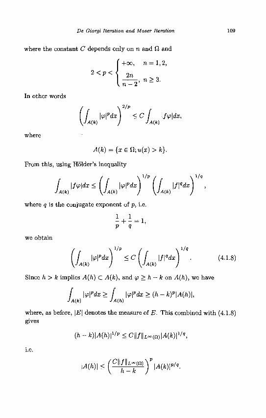
De Giorgi Iteration and Moser Iteration 109
where the constant C depends only on n and si and
{ +00, n = l ,2,
In other words
2/P
' ~ ' IX, f \<p\»dx) <C f \f<p\da jA(k) I JA(k) >A(k) / JA(k)
where
A(k) = {x e fi;u(x) > fc}.
Prom this, using Holder's inequality
/ \f<p\dx<(f \<p\pdx) If |/|«dx) , ./Ac*:) \v,4(it) y \-/>i(fc) y
where 9 is the conjugate exponent of p, i.e.
i + i-i. P Q
we obtain
\ i /p / \ 1/9 ( / " M ' d x ) < C ( / l/l'efa] . (4.1.8) V-^w y v^(fc) y
Since h > k implies A(h) C A(k), and (p> h — k on A(h), we have
/ M p d i > / | ^ | p ^ > ( / i - f c ) p | ^ ( / i ) | ,
where, as before, \E\ denotes the measure of E. This combined with (4.1.8) gives
(h-k)\A(h)\1'p<C\\f\\Lo.(a)\A(k)\1/'>,
i.e.
\A{h)\<(CU^~W)YlA{k)lv/<,.
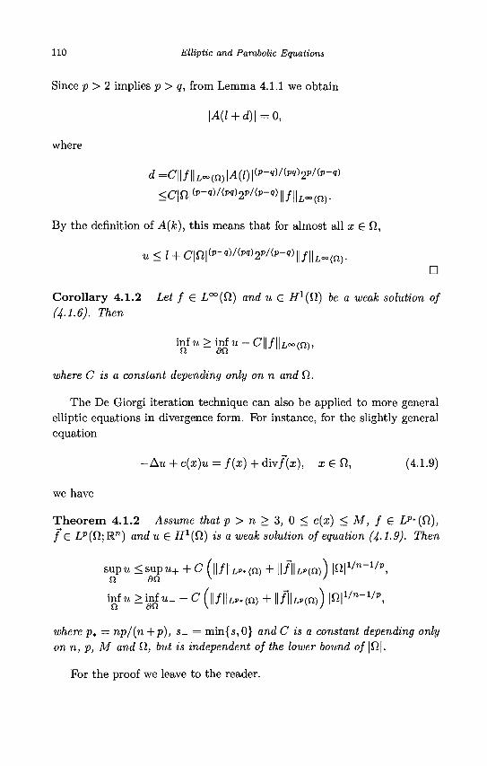
110 Elliptic and Parabolic Equations
Since p > 2 implies p > q, from Lemma 4.1.1 we obtain
\A(l + d)\=0,
where
^=C||/||L~(n)|^(0l(p_<') /(p9)2p/(p-9)
<C|fi|(P-«)/<«)2P/(P-«)||/| |L- (n).
By the definition of A(k), this means that for almost all x £ fi,
« < i + c|n|^-«)/^2"/<"-«)||/||L=o(n). n
Corollary 4.1.2 Lei / € L°°(0) and u £ /f1(fi) be a weafc solution of (4.1.6). Then
i n f u > i n f u - C | | / | | L o o ( n ) ,
where C is a constant depending only on n and 0 .
The De Giorgi iteration technique can also be applied to more general elliptic equations in divergence form. For instance, for the slightly general equation
- A u + c(x)u = f(x) + divf(x), i e ( l , (4.1.9)
we have
Theorem 4.1.2 Assume that p > n > 3, 0 < c(x) < M, f € Lp*(fi), / £ Lp(fi;R") andu £ iJ1(f2) is a weak solution of equation (4-1.9). Then
supu < s u p u + + C (||/||LP.(n) + ||/1lLP(n)) | f i | 1 / n " 1 / p ,
inf u >mf u_ - C (||/||LP.(n) + | | / | | L ^ ) ) | 0 | 1 / n " 1 / p ,
where p* = np/(n + p), s_ = min{s,0} and C is a constant depending only on n, p, M and Q, but is independent of the lower bound of |fi|.
For the proof we leave to the reader.
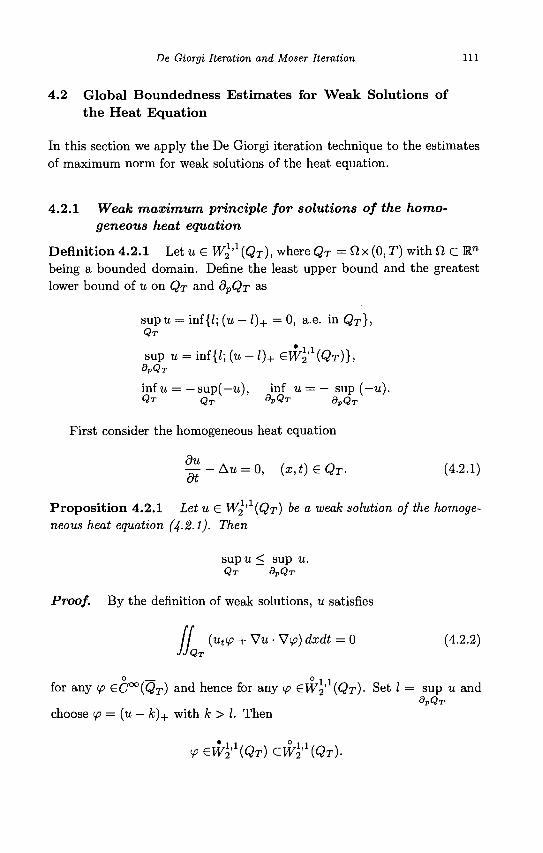
De Giorgi Iteration and Moser Iteration 111
4.2 Globa l B o u n d e d n e s s E s t i m a t e s for W e a k So lu t ions of
t h e H e a t E q u a t i o n
In this section we apply the De Giorgi iteration technique to the estimates
of maximum norm for weak solutions of the heat equation.
4.2 .1 Weak maximum principle for solutions of the homo
geneous heat equation
Def in i t ion 4 .2 .1 L e t u e W2hl(QT), where QT = ftx(0,T) with ft C W1
being a bounded domain. Define the least upper bound and the greatest
lower bound of u on QT and dpQr as
s u p u = inf{Z; (u — l)+ = 0, a.e. in QT}, QT
sup u = inf{/; (u - l)+ eW2' (QT)}, dpQr
inf u = — sup(—u), inf u — — sup (—u). QT QT dpQT dpQT
First consider the homogeneous heat equation
flit ^ - A u = 0, (x,t)eQT- (4.2.1)
P r o p o s i t i o n 4 .2 .1 Let u £ W2' (QT) be a weak solution of the homoge
neous heat equation (4-2.1). Then
s u p u < sup u. QT BVQT
Proof. By the definition of weak solutions, u satisfies
/ / (ut<p + V u • Vy>) dxdt = 0 (4.2.2)
JJQT
o ° 1 1 for any ip &C°°(QT) and hence for any <p £W2 (QT)- Set I = sup u and
9VQT
choose (p = (u — k)+ with k > I. Then
<P £WY(QT) CWl'^Qr).
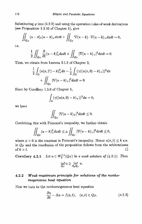
112 Elliptic and Parabolic Equations
Substituting <p into (4.2.2) and using the operation rules of weak derivatives (see Proposition 1.3.10 of Chapter 1), give
/ / (u - k)t(u - k)+dxdt + W(u-k)-V(u-k)+dxdt = 0, JJQT JJQT
i.e.
- if —(u-k)%dxdt+ [J \V(u-k)+\2dxdt = Q. IQT
Ul JJQT
Thus, we obtain from Lemma 3.1.2 of Chapter 3,
\ I (u(x, T) - k)\dx - \ \ (7((u(ar, 0) - k)+))2dx «/ 12 </ S2
+ ff \\7(u-k)+\2dxdt = 0. JJQT 'QT
Since by Corollary 1.5.6 of Chapter 1,
/ ( 7 ( K a ; , 0 ) - f c ) + ) ) 2 d a ; = 0,
we have
/ / \V(u-k)+\2dxdt<0. JJQT
Combining this with Poincare's inequality, we further obtain
/ / (u - k)\dxdt < M / / |V(u - k)+\2dxdt < 0, JJQT JJQT
where /x > 0 is the constant in Poincare's inequality. Hence u(x,t) < k a.e. in QT and the conclusion of the proposition follows from the arbitrariness of k > I. D
Corollary 4.2.1 Let u G W^iQr) be a weak solution of (4-2.1). Then
inf u > inf u. QT 9PQT
4.2.2 Weak maximum principle for solutions of the nonho-mogeneous heat equation
Now we turn to the nonhomogeneous heat equation
^ - A u = f(x,t), (x,t)€QT. (4.2.3)
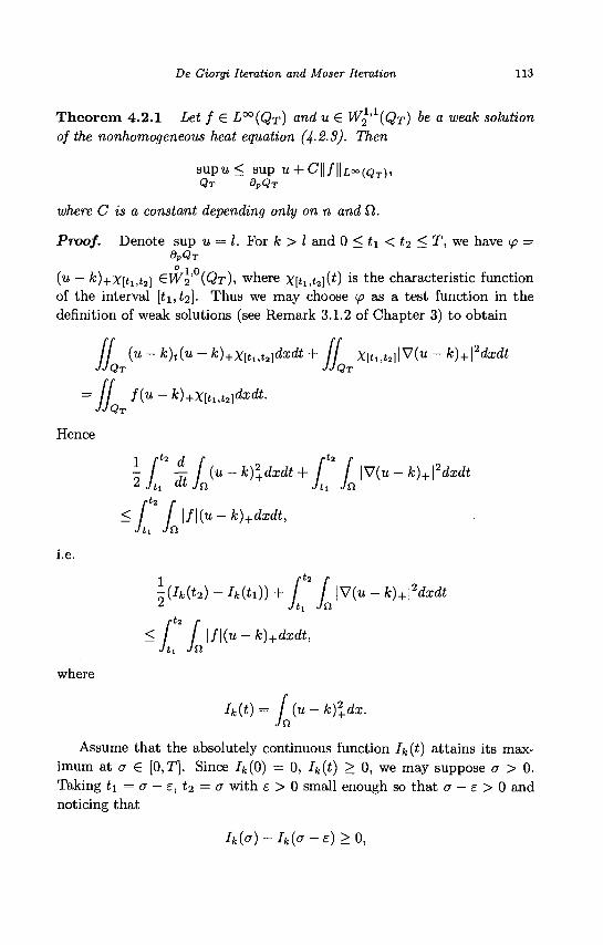
De Giorgi Iteration and Moser Iteration 113
Theorem 4.2.1 Let f £ L°°(QT) and u £ W2' (QT) be a weak solution of the nonhomogeneous heat equation (4-2.3). Then
s u p u < sup u + C||/ | |L<»(Q r ), QT 9PQT
where C is a constant depending only on n and il.
Proof. Denote sup u = 1. For k > I and 0 < t\ < t2 < T, we have <p = dpQT
O < n
(u — k)+X[t1,t2] GWV (QT), where X[ti,t2]W 1S ^e characteristic function
of the interval [ t i , ^ ] . Thus we may choose tp as a test function in the definition of weak solutions (see Remark 3.1.2 of Chapter 3) to obtain
/ / (u-k)t(u-k)+X[t1,t2]dxdt+ / / X[tl,t2]|V(u - k)+\2dxdt JJQT JJQT
JJc 'QT
Hence
QT JJQT
f(u-k)+X[tut2\dxdt.
o / H (u-k)2+dxdt+ / / \X7(u-k)+\2dxdt 2 Jti dt Jn Jti Jn
< 1^ I \f\(u-k)+dxdt, Jti Jn
i.e.
where
\(ik(t2) - Mil)) + r i iv(u - k)+\2dxdt 1 Jti Jn
< [* I \f\(u - k)+dxdt, Jti Jn
Ik(t)= / ( u - k ) \ d x . Jn
Assume that the absolutely continuous function Ik(t) attains its maximum at a e [0,T]. Since Jfe(0) = 0, h(t) > 0, we may suppose a > 0. Taking ti = a — e, t2 = o with e > 0 small enough so that a — e > 0 and noticing that
h(°) - h(°-~ s) > 0,
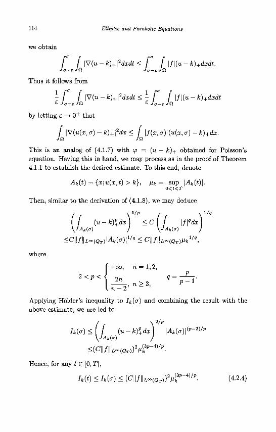
114 Elliptic and Parabolic Equations
we obtain
f f |V(« - k)+\2dxdt < f f \f\{u - k)+dxdt. J<7—£ JQ J a—E JQ
Thus it follows from
- / / l v ( u - k)+\2dxdt <- f [ \f\(u - k)+dxdt e Jcr-e Jfl £ J as JQ,
by letting e —> 0+ that
/ \V{u(x,a)-k)+\2dx < / \f(x,a)\(u(x,a) - k)+dx. JO. JO.
This is an analog of (4.1.7) with (p = (u — k)+ obtained for Poisson's equation. Having this in hand, we may process as in the proof of Theorem 4.1.1 to establish the desired estimate. To this end, denote
Ak(t) = {x;u(x,t)> k}, \ik = sup \Ak(t)\. 0<t<T
Then, similar to the derivation of (4.1.8), we may deduce
( / (u-k)p+dx) <C\ [ \f\"dx)
\JAk(cT) J \JAk(cr) ) <C\\}\\L-{QT)\Ak{o)\V« < C||/||L~(QT)/ifc
1/9, where
+oo, n = 1,2,
2 <p< < 2 n n > 3 , Q P-1'
U - 2
Applying Holder's inequality to Ik(a) and combining the result with the above estimate, we are led to
h{°) <( [ (« - kf+dx J \Ak(a)\^-^p
\JAk(a) J
<(cn/ik~(QT))2/43p-4)/p.
Hence, for any t € [0, T],
/*(*) < hi*) < (C\\f\\L~(QT))2tfp-i)/p. (4.2.4)
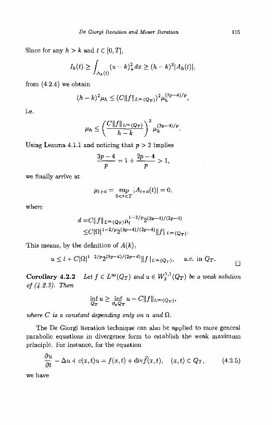
De Giorgi Iteration and Moser Iteration 115
Since for any h > k and t £ [0, T],
h(t) > f (u - k)2+dx >(h- k)2\Ah(t)\,
JAh(t)
from (4.2.4) we obtain
(h-k)W<(C\\f\\L^QT))2^4)/p,
i.e.
(C\\f\\ L^iQrA (3p-4)/p
Using Lemma 4.1.1 and noticing that p > 2 implies
P P
we finally arrive at
/xj+d = sup \Ai+d(t)\ = 0 , 0<t<T
where
rf=G||/ll^(QT)^-2/P2(3p-4)/(2p-4)
^cifil1-2/^^-4)/^-4)!!/!!^^).
This means, by the definition of A(k),
uKl + ClQf-V^-W^Wfh^Q^, a.e. i n Q r . Q
Corollary 4.2.2 Let f £ L°°(QT) and u £ W^' ( Q T ) &e a weofc solution of (4.2.3). Then
}?*"-/>"# U - C 1 I / I U ~ ( Q T ) . Q T O P Q T
where C is a constant depending only on n and 0 .
The De Giorgi iteration technique can also be applied to more general parabolic equations in divergence form to establish the weak maximum principle. For instance, for the equation
du -* — -Au + c(x,t)u = f(x,t)+divf(x,t), (x,t)eQT, (4.2.5)
we have
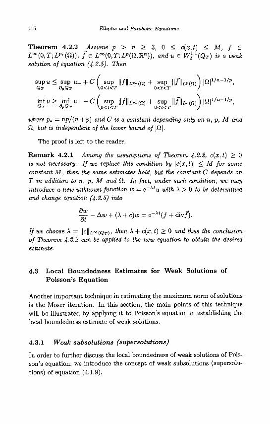
116 Elliptic and Parabolic Equations
Theorem 4.2.2 Assume p > n > 3, 0 < c(x,t) < M, f e L°°(0,T;LP'(D.)), fe Loo(0,T;IA'(Q,Rn)), and u € W\<X{QT) is a weak solution of equation (4-2.5). Then
s u p u < s u p u + + c f sup | | / | | i , . ( n ) + sup | | / |UP(n)) M 1 / n _ 1 / p , QT dpQT \0<t<T 0<t<T /
mfu> inf u . - c ( sup | | / | | L , . ( n ) + sup ll/IU^n) V | 1 / n - 1 / p , QT OPQT \0<t<T 0<t<T J
where p* = np/(n+p) and C is a constant depending only on n, p, M and Cl, but is independent of the lower bound of |fi|.
The proof is left to the reader.
Remark 4.2.1 Among the assumptions of Theorem 4-2.2, c(x,t) > 0 is not necessary. If we replace this condition by \c(x,t)\ < M for some constant M, then the same estimates hold, but the constant C depends on T in addition to n, p, M and Q. In fact, under such condition, we may introduce a new unknown function w = e_ A tu with A > 0 to be determined and change equation (4-2.5) into
^ - Aw + (A + c)w = e - A t ( / + div/). at
If we choose A = ||c||i,°o(Qr), then A + c(x,t) > 0 and thus the conclusion of Theorem 4-2-2 can be applied to the new equation to obtain the desired estimate.
4.3 Local Boundedness Estimates for Weak Solutions of Poisson's Equation
Another important technique in estimating the maximum norm of solutions is the Moser iteration. In this section, the main points of this technique will be illustrated by applying it to Poisson's equation in establishing the local boundedness estimate of weak solutions.
4.3.1 Weak subsolutions (supersolutions)
In order to further discuss the local boundedness of weak solutions of Poisson's equation, we introduce the concept of weak subsolutions (supersolutions) of equation (4.1.9).
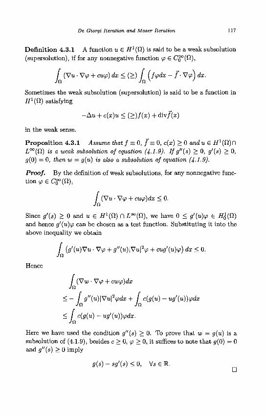
De Giorgi Iteration and Moser Iteration 117
Definition 4.3.1 A function u € H1^) is said to be a weak subsolution (supersolution), if for any nonnegative function <p £ Co°(ft),
/ (Vu • V<p + cuip) dx < (>) / (fipdx - / • V(p) dx.
Sometimes the weak subsolution (supersolution) is said to be a function in if1(fi) satisfying
-Au + c(x)u < (>)/(x) + div/(x)
in the weak sense.
Proposition 4.3.1 Assume that f = 0, / = 0, c(x) > 0 andu e if1(f2)n L°°(Q) is a weak subsolution of equation (4-1.9). If g"(s) > 0, g'(s) > 0, 3(0) = 0, then w = g(u) is also a subsolution of equation (4-1.9).
Proof. By the definition of weak subsolutions, for any nonnegative function tp G Cg°(fi),
/ (Vu • Vy> + cwp)dx < 0. n
Since g'(s) > 0 and u <E tf^fi) n L°°(D,), we have 0 < g'{u)<p € H^(Sl) and hence g'(u)<p can be chosen as a test function. Substituting it into the above inequality we obtain
/ (g'(u)Vu • V<£> + g"(u)\Vu\2<p + cug'(u)tp) dx < 0. Jo,
Hence
/ (Vu; • Vtp + cwip)dx Jn
<- g"(u)\Vu\2<pdx + / c(g(u) - ug'(u))<pdx Jn Jn
< / c{g{u) - ug'(u))ipdx. Jn
Here we have used the condition g"(s) > 0. To prove that w = g(u) is a subsolution of (4.1.9), besides c > 0, cp > 0, it suffices to note that 5(0) = 0 and g"{s) > 0 imply
g(s) - sg'(s) < 0, Vs e R. D
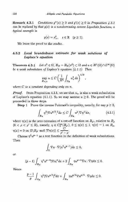
118 Elliptic and Parabolic Equations
Remark 4.3.1 Conditions g"(s) > 0 and g'(s) > 0 in Proposition 4-3-1 can be replaced by that g(s) is a nondecreasing convex Lipschitz function; a typical example is
g(s) = sp+, s e R ( p > l ) .
We leave the proof to the reader.
4.3.2 Local boundedness estimate for weak solutions of Laplace's equation
Theorem 4.3.1 Let x° & Q, BR = BR(x°) Cfl andut H1 (SI) n L°°(0.) be a weak subsolution of Laplace's equation (4-1.1). Then
sup u < C I —— / u+dx BR,2 \ R n JBR
— / u2,t 1/2
where C is a constant depending only on n.
Proof. Prom Proposition 4.3.1, we see that u+ is also a weak subsolution of Laplace's equation (4.1.1). So we may assume u > 0. The proof will be proceeded in three steps.
Step 1 Prove the inverse Poincare's inequality, namely, for any p > 2,
f r)2\Vup'2\2dx < C [ up\Vn\2dx, (4.3.1) JBR JBR
where rj(x) is the zero extension of a cut-off function on Bp>, relative to Bp
(0 < p < pf < R), namely, rj € C$>(Bp,), 0 < n(x) < 1, n(x) = 1 on Bp,
r](x) = 0 on Cl\Bp> and \S7n(x)\ < — .
Choose 7y2up_1 as a test function in the definition of weak subsolutions. Then
/ Vu-V(n2up-l)dx<0, Jn
(p-l) f n2up-2\Vu\2dx + 2 J riup-lVu • Vrjdx < 0. J BR J BR
^ ^ / ri2\Vup/2\2dx + f r)up'2Vup/2 • Vrjdx < 0. P JBR JBR
or
Hence
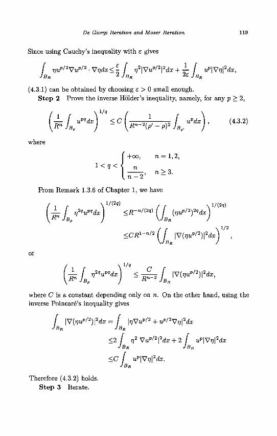
De Giorgi Iteration and Moser Iteration 119
Since using Cauchy's inequality with e gives
/ r,up'2^up'2 -S/r]dx<^ [ r)2\Vup/2\2dx + l- [ up\Wr]\2dx, JBR
2 JBR
2e JBR
(4.3.1) can be obtained by choosing e > 0 small enough. Step 2 Prove the inverse Holder's inequality, namely, for any p > 2,
i-z- [ upqdx) <C[„ * r= f updx), (4.3.2)
\RnJBp ) ~ \Rn-2(p,-p)2JBl>, J y ' where
+oo, n = 1,2,
n n > 3.
1 <q < <
. n - 2 '
Prom Remark 1.3.6 of Chapter 1, we have
/ , , \ 1 / ( 2 < j ) / , \i/(2g) _ L / rpundx] <R-n'<*>U W'2)*>dx\
<CRi-"/*([ \V{riup/2)\2dx\ ,
or
where C is a constant depending only on n. On the other hand, using the inverse Poincare's inequality gives
/ \V(r]up/2)\2dx = f \r)Vup'2 + up/2VV\2dx J BR J BR
<2 [ r]2\Vup/2\2dx + 2 [ up\Vr)\2dx JBR JBR
<C [ up|Vry|2
JBR
Therefore (4.3.2) holds. Step 3 Iterate.
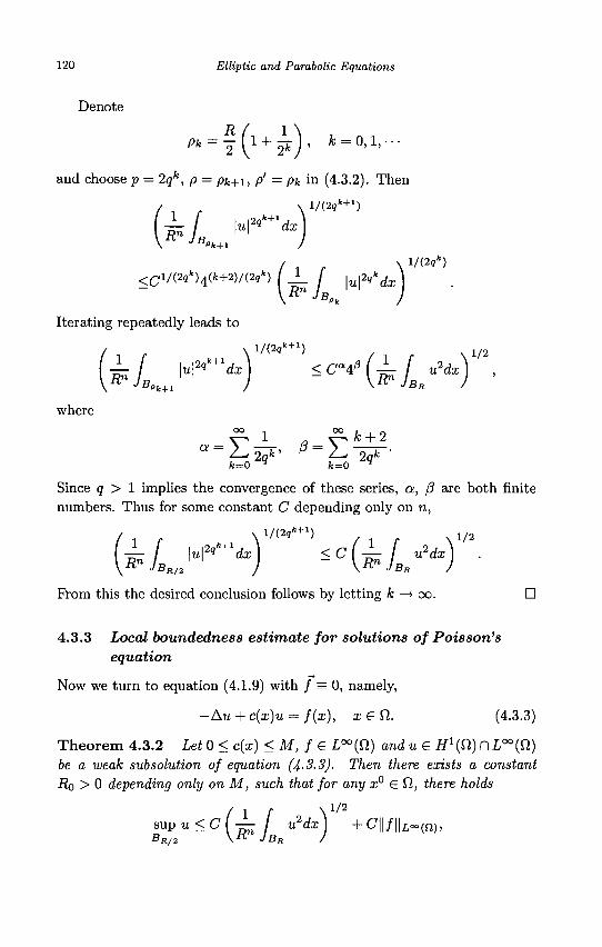
120 Elliptic and Parabolic Equations
Denote
and choose p = 2qk, p = pk+i, p' = pk in (4.3.2). Then
\ i / ( 2 g f c + 1 )
RnJB. „ . \u\2"k+1dx
/ N V<2«*>
Iterating repeatedly leads to
/ i /• \ 1 / { 2 q k + 1 ) S i r \ V2
where OO - OO fc + 2
2 o f c ' ^ ^ 2o fc '
Since 9 > 1 implies the convergence of these series, a, (3 are both finite numbers. Thus for some constant C depending only on n,
/ v l / ( 2 9f c + 1 ) 1/2
Prom this the desired conclusion follows by letting k —• oo. •
4.3.3 Local boundedness estimate for solutions of Poisson's equation
Now we turn to equation (4.1.9) with / = 0, namely,
-Au + c(x)u = f(x), x G f i . (4.3.3)
Theorem 4.3.2 Let 0 < c(x) <M, f G L°°(ft) and u G if 1(f i )nL°°(n) 6e a weafc subsolution of equation (4-3.3). Then there exists a constant Ro > 0 depending only on M, such that for any x° G Cl, there holds
s u p u < C ( — / u2dx) +C| | / | | L oo ( n ) , B R / 2 V-" JBR J
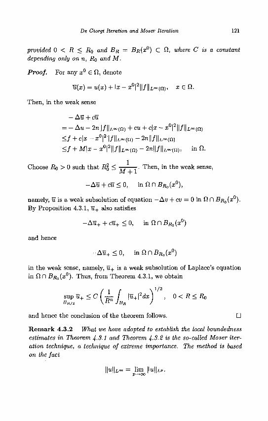
De Giorgi Iteration and Moser Iteration 121
provided 0 < R < R0 and BR = BR(X°) C Q, where C is a constant depending only on n, RQ and M.
Proof. For any x° e £1, denote
u(x) = u(x) + \x- z°|2||/||L=c(n), x € ft.
Then, in the weak sense
— Au + cu
= -Au- 2n||/ | |Loo (n) +cu + c\x - x°|2||/||L°°(fi)
<f + c\x - x°|2 | | / | |L Oc ( n ) - 2n | | / | | L - ( n)
< / + M\x - x°|2 | | / | |L=c (n ) - 2n| | / | |L» (n), in SI.
Choose i?o > 0 such that RQ < ——-. Then, in the weak sense,
-Au + cu<0, mQr\BRo(x°),
namely, u is a weak subsolution of equation —Av + cv = 0 in Q D BR0(X°).
By Proposition 4.3.1, u+ also satisfies
- A u + + cu+ < 0, in Q, n Bfl0 (x°)
and hence
- A u + < 0 , mQ,nBRo(x0)
in the weak sense, namely, u+ is a weak subsolution of Laplace's equation in fi n jBfl0(a;0). Thus, from Theorem 4.3.1, we obtain
sup u+ < C ( — / \u+\2dx ] , 0 < R < Ro Ban +~ WJBJ + ' J
\ l / 2 i p u + <C[ -^ I \u+\zdo
BR
and hence the conclusion of the theorem follows. •
R e m a r k 4.3.2 What we have adopted to establish the local boundedness estimates in Theorem 4-3.1 and Theorem 4-3.2 is the so-called Moser iteration technique, a technique of extreme importance. The method is based on the fact
IMU°o = lim \\U\\LP-
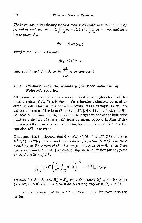
122 Elliptic and Parabolic Equations
The basic idea in establishing the boundedness estimates is to choose suitably Pk and pk such that po = R, lim pk = R/2 and lim pk = +00, and then
fe—»oo fe—»oo
try to prove that
Ak = \\u\\L'k(BPk)
satisfies the recursive formula
Ak+1 < Ca"Ak
00
with otk > 0 such that the series VJ ctk is convergent. fc=o
4.3.4 Estimate near the boundary for weak solutions of Poisson's equation
All estimates presented above are established in a neighborhood of the interior points of Q. In addition to these interior estimates, we need to establish estimates near the boundary points. As an example, we will do this for a domain of the form Q+ = {x € M.n; |XJ| < 1 (1 < i < n),xn > 0}. For general domains, we may transform the neighborhood of the boundary point to a domain of this special form by means of local flatting of the boundary. Of course, after a local flatting transformation, the shape of the equation will be changed.
Theorem 4.3.3 Assume that 0 < c(x) < M, f £ L°°(Q+) and u € H1(Q+) n L°°(Q+) is a weak subsolution of equation (4-3.3) with trace vanishing on the bottom of Q+, i.e. ju(x\,--- ,a;„_i,0) = 0. Then there exists a constant Ro £ (0,1] depending only on M, such that for any point x° on the bottom of Q+,
sup u<c(— I u2dx\ + C | | / | | L ~ ( Q + ) , BR/2 \ R /
provided 0 < R < RQ and B^ = B+(x°) C Q+, where B^(x°) = BR(x°) n {x s Rn;xn > 0} and C is a constant depending only on n, Ro and M.
The proof is similar as the one of Theorem 4.3.2. We leave it to the reader.
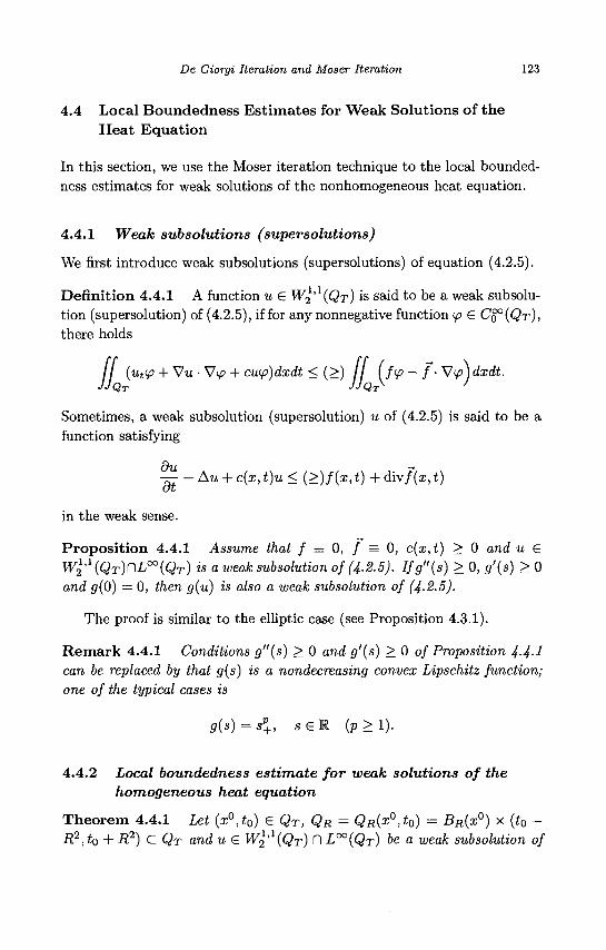
De Giorgi Iteration and Moser Iteration 123
4.4 Local Boundedness Estimates for Weak Solutions of the Heat Equation
In this section, we use the Moser iteration technique to the local boundedness estimates for weak solutions of the nonhomogeneous heat equation.
4.4.1 Weak subsolutions (supersolutions)
We first introduce weak subsolutions (supersolutions) of equation (4.2.5).
Definition 4.4.1 A function u G W^iQr) is said to be a weak subsolution (supersolution) of (4.2.5), if for any nonnegative function <p G CQ° (QT) , there holds
/ / (ut<p + Vu-V<p + cu(p)dxdt < (>) / / (ftp - f- Vip)dxdt. JJQT JJQT^ '
Sometimes, a weak subsolution (supersolution) u of (4.2.5) is said to be a function satisfying
OVL ~*
— - Au + c(x, t)u < ( > ) / ( ! , t) + div/(x, t)
in the weak sense.
Proposition 4.4.1 Assume that f = 0, / = 0, c(x,t) > 0 and u G W2
1 '1(gr)nL0 0(Qr) is a weak subsolution of (4.2.5). Ifg"(s) > 0, g'(s) > 0 and g(0) = 0, then g(u) is also a weak subsolution of (4-2.5).
The proof is similar to the elliptic case (see Proposition 4.3.1).
R e m a r k 4.4.1 Conditions g"{s) > 0 and g'(s) > 0 of Proposition 4-4-1 can be replaced by that g(s) is a nondecreasing convex Lipschitz function; one of the typical cases is
g(s) = sp+, s e R ( p > l ) .
4.4.2 Local boundedness estimate for weak solutions of the homogeneous heat equation
Theorem 4.4.1 Let (x°,t0) G QT, QR = QR(x°,t0) = BR(x°) x {t0 -R2,t0 + R2) C QT and u G Wl'1(QT) n L°°(QT) be a weak subsolution of
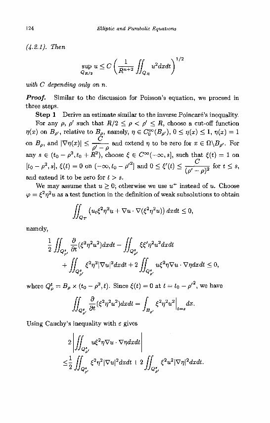
124 Elliptic and Parabolic Equations
(4-2.1). Then
ST~C(n^l/dxdt)"2
with C depending only on n.
Proof. Similar to the discussion for Poisson's equation, we proceed in three steps.
Step 1 Derive an estimate similar to the inverse Poincare's inequality. For any p, p' such that R/2 < p < p' < R, choose a cut-off function
rj(x) on Bpi, relative to Bp, namely, n G CQ°(BP>), 0 < n(x) < 1, r](x) = 1
on Bp, and |V^(x)| < — and extend 77 to be zero for x G Q\Bpi. For
any s G (to — P2,h + R2), choose £ G C°°(—00, s], such that £(t) = 1 on
[t0 - p2,s], £(t) = 0 on (-00, t0 - p'2] and 0 < C(t) < — ^ for t < s, (P - P)
and extend it to be zero for t > s. We may assume that u > 0; otherwise we use u+ instead of u. Choose
ip = £2n2u as a test function in the definition of weak subsolutions to obtain
IQ
namely,
/ / {ut£"n2u + Vu • V ( £ V u ) ) dxdt < 0, JJQT
\jj. Wt{ev2u2)dxdt~U s ti'^dxdt p' p'
+ if tW\Vu\2dxdt + 2 if u^nVu • Vrjdxdt < 0, *<pi pi
where Qp = Bp x (to - p2,t). Since f (t) = 0 at t = t0 - p' , we have
[f ±L(Z2r,2u2)dxdt = f ZWu2 dx. JJQ* or JB t=s
Using Cauchy's inequality with e gives
2 / / u£2rjVu • Vrjdxdt
p'
-If Z2r,2\Vu\2dxdt + 2 ff Z2u2\Vr)\2dxdt. <-~2
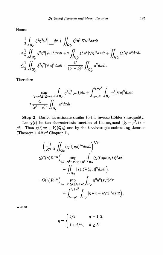
De Giorgi Iteration and Moser Iteration 125
Hence
\ [ £ W dx+ [[ er?\Vu\2dxdt
<- ff tW\Vu\2dxdt + 2 / / £2u2\Vr)\2dxdt+ ff tt'r}2u2dxdt 2 JJQp JJQ^ JJQS^
<\ ff £2ri2\Vu\2dxdt+ , C / / u2dxdi. 2 y jQ' , (.P _ P) .A/Q',
Therefore
/• rto+P r sup / r)2u2(x,t)dx+ / / T72|Vu|2dxdt
to-p2<t<to+p2JB0, Jto-p2 JBp,
<, . ^ xo / / u2da:eft. JJQj
C_ '{P'-PYJJQ
Step 2 Derive an estimate similar to the inverse Holder's inequality. Let x (0 be the characteristic function of the segment [to — p2,to +
p2}. Then x{t)rlu G V^Q/j) and by the t-anisotropic embedding theorem (Theorem 1.4.2 of Chapter 1),
(sw/0„wt) '" )2w 'r <C(n)R-n( sup / (x(t)7?u(a:,t))2dx
^t0-R2<t<t0+R2 JBR
+ IJ \X(t)V(Vu)\2dxdt).
=C{n)R7n( sup / r)2u2(x,t)dx ^t0-p
2<t<t0+p2 JB-i
rto+P r . + / / \r]Vu + uVr)\2dxdt),
where
5/3, n = l ,2,
1 + 2/ra, n > 3.
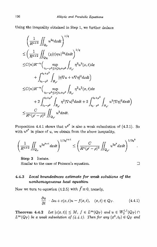
126 Elliptic and Parabolic Equations
Using the inequality obtained in Step 1, we further deduce
1/9
'Qt j
Dn+2
JJ {X{t)rjufdxd^
<C(n)R-n( sup / r?u2{x,t)dx V *o-p 2 <t<*o+p 2 JBp,
t-to+p r . + / / \r]Vu + uVri\2dxdt)
Jto-p2 JBp, ' <C{n)R-n( sup / rj2u2(x,t)dx
^t0-p2<t<t0+p2 JBp,
rto+p r fto+p2 /• . + 2 / / n2\Wu\2dxdt + 2 / / u2\Vn\2dxdt)
Jto-p2 JB„, Jt0-p2 JB„, '
< „ _ , ^ — / / U 2 d l ^ . Rn{p'-P)2 JJQ P
Proposition 4.4.1 shows that u9 is also a weak subsolution of (4.2.1). So with uq in place of u, we obtain from the above inequality,
/ x l/2qk+1 / v l/2qk
Step 3 Iterate. Similar to the case of Poisson's equation. •
4.4.3 Local boundedness estimate for weak solutions of the nonhomogeneous heat equation
Now we turn to equation (4.2.5) with / = 0, namely,
Qu — -Au + c(x,t)u = f(x,t), (x,t)GQT. (4.4.1)
Theorem 4.4.2 Let \c(x,t)\ < M, f £ L°°(QT) and u £ W2M(Qr) f~l
L°°(QT) be a weak subsolution of (4-4-1)- Then for any (x°,to) € QT and
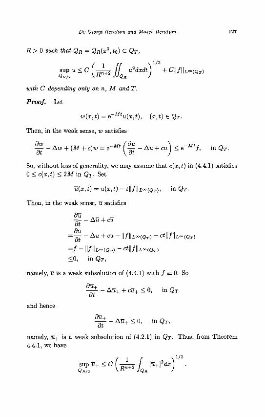
De Giorgi Iteration and Moser Iteration 127
R > 0 such that QR = QR{X°, t0) C QT,
sup u<c(j±^ IJ u2dxdt^j + C | | / | | L O O W T )
1/2 U<C { -^y; /I U2dxdt }
QR/2
with C depending only on n, M and T.
Proof. Let
w(x,t) = e~Mtu(x,t), (x,t)eQT-
Then, in the weak sense, w satisfies
^ - Aw + (M + c)w = e-Mt (^-Au + cu]< e~Mtf, in QT. at \at )
So, without loss of generality, we may assume that c(x, t) in (4.4.1) satisfies 0<c(x,t) <1M in QT. Set
u(x,t) =u{x,t)-t\\f\\Loc{QT), in QT-
Then, in the weak sense, u satisfies
&& A — —
— Au + cu at dit
=~di ~Au + cu~ H/IU~(QT) _ ct\\f\\L^(QT)
= / - II/IU»(QT) - CtWfh^iQr)
<0, in QT,
namely, u is a weak subsolution of (4.4.1) with / = 0. So s-i
—^- — Au+ + cu+ < 0, in QT (so
and hence
— - Au+ < 0, in QT, dt
namely, u+ is a weak subsolution of (4.2.1) in QT- Thus, from Theorem 4.4.1, we have
ss^-c(^LMdx)
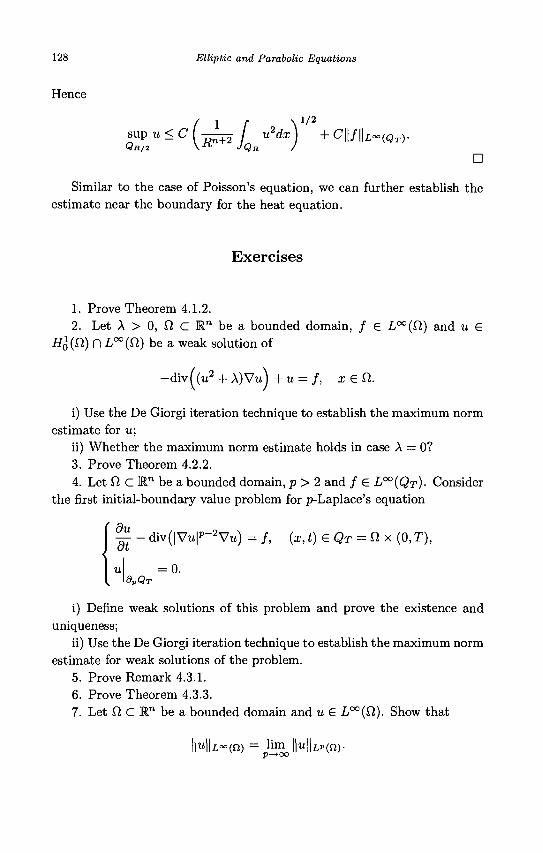
128 Elliptic and Parabolic Equations
Hence
1/2
sup u < C ( - L j f u2dx) + C | | / | | L - ( Q T ) . QR/2 V-0,
JQR /
• Similar to the case of Poisson's equation, we can further establish the
estimate near the boundary for the heat equation.
Exercises
1. Prove Theorem 4.1.2. 2. Let A > 0, n C R" be a bounded domain, / G L°°(fi) and u G
HQ(Q) n L°°(fi) be a weak solution of
-d iv ( (u 2 + A)Vu) +u = f, i e f i .
i) Use the De Giorgi iteration technique to establish the maximum norm estimate for u;
ii) Whether the maximum norm estimate holds in case A = 0? 3. Prove Theorem 4.2.2. 4. Let 0 C t n be a bounded domain, p > 2 and / G L°°(QT)- Consider
the first initial-boundary value problem for p-Laplace's equation
— - divfl V u r 2Vu) = / , (x, i ) G Q r = O x (0, T),
= 0. dPQx
i) Define weak solutions of this problem and prove the existence and uniqueness;
ii) Use the De Giorgi iteration technique to establish the maximum norm estimate for weak solutions of the problem.
5. Prove Remark 4.3.1. 6. Prove Theorem 4.3.3. 7. Let Q C Kn be a bounded domain and u G L°°(Q). Show that
IMU~(n) = limJ|u||LP(n).
De Giorgi Iteration and Moser Iteration 129
8. Let u\ and U2 € HQ(Q) >e a w e a k solution and a weak subsolution of Poisson's equation
—Au = / , i £ f i ,
where Q C R" is a bounded domain and / € L2(Q,). Show that
ui(x) > U2{x), a.e. x € £1.
9. Prove that u £ W2' (QT) is a weak solution of the equation
— -Au + c(x,t)u = f, (x,t)eQT = flx(0,T)
if and only if u is both the weak supersolution and the weak subsolution of the equation, where fi C W1 is a bounded domain, c S L°°(QT) and / G L2(QT).
10. Prove Proposition 4.4.1 and Remark 4.4.1. 11. Let u G W2' (QT) n L°°(QT) be a weak solution of the equation
W " div ( ( ^ r l ) V u ) + < X ^ U = *> (x'*)e gr = fi x (°'T) where Q. C R" is a bounded domain, c £ L°°(QT) and / € L2(QT). Use the Moser iteration technique to derive the local boundedness estimate for u.
12. Use the Moser iteration technique to derive the local boundedness estimate near the boundary for weak solutions of the heat equation.

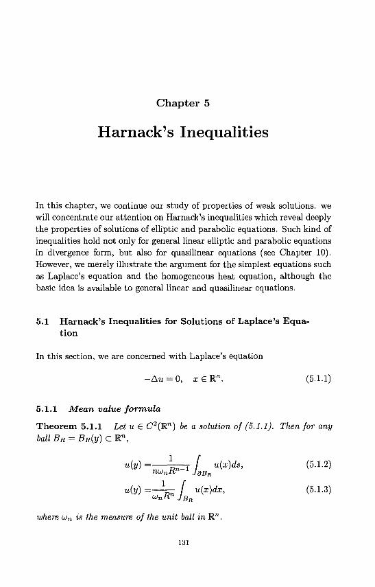
Chapter 5
Harnack's Inequalities
In this chapter, we continue our study of properties of weak solutions, we will concentrate our attention on Harnack's inequalities which reveal deeply the properties of solutions of elliptic and parabolic equations. Such kind of inequalities hold not only for general linear elliptic and parabolic equations in divergence form, but also for quasilinear equations (see Chapter 10). However, we merely illustrate the argument for the simplest equations such as Laplace's equation and the homogeneous heat equation, although the basic idea is available to general linear and quasilinear equations.
5.1 Harnack's Inequalities for Solutions of Laplace's Equation
In this section, we are concerned with Laplace's equation
- A u = 0, x£Rn. (5.1.1)
5.1.1 Mean value formula
Theorem 5.1.1 Let u € C2(Rn) be a solution of (5.1.1) ball BR = BR{y) C Rn ,
u(y) =~ ^T=T / u(x)ds, nunR
n l J9BR
u(y) =—5^ / u(x)dx,
where un is the measure of the unit ball in M.n.
Then for any
(5.1.2)
(5.1.3)
131
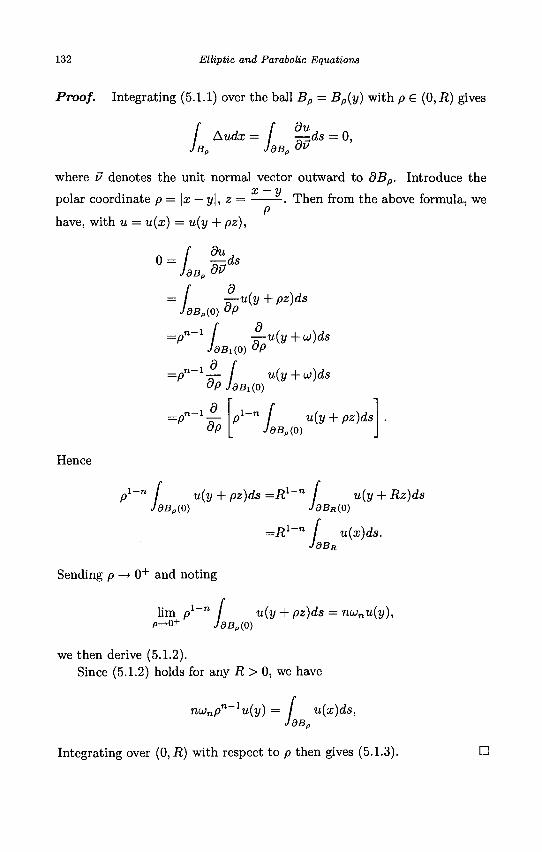
132 Elliptic and Parabolic Equations
Proof. Integrating (5.1.1) over the ball Bp = Bp(y) with p € (0, R) gives
/ Audx = / JB„ Jdi
Audx = I Tr^ds — 0, IB0 JdBB du
where v denotes the unit normal vector outward to dBp. Introduce the
polar coordinate p=\x — y\,z =
have, with u = u(x) = u(y + pz),
0
x-y Then from the above formula, we
Jdi IdB, dv
-L aBp(o)
d_ dp
u(y + pz)ds
7 JdBx
(0)
d_ dp
u(y + u)ds
„ n - i d =p- '— / u(y + u)ds
dp JdB^o)
dp p1 n u(y + pz)ds
JdBp(0)
Hence
pl~n ( u(y + pz)ds =R1~n I u{y + Rz)ds JdBp(o) JdBR(.o)
= i ? 1 - " / u(x)ds. JdBR
Sending p —• 0 + and noting
lim pl~n / u(y + pz)ds = nunu(y), P-+0+ JdBp(0)
we then derive (5.1.2). Since (5.1.2) holds for any R > 0, we have
ncjnpn~1u(y) = / u(x)ds,
JdBp
Integrating over (0,-R) with respect to p then gives (5.1.3). •
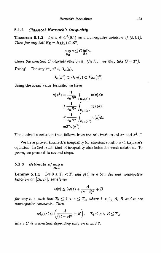
Harnack's Inequalities 133
<
5.1.2 Classical Harnack's inequality
Theorem 5.1.2 Let u € C2(Rn) be a nonnegative solution of (5.1.1). Then for any ball BR = BR(y) C M.n,
sup u < C inf u, BR BR
where the constant C depends only on n. (In fact, we may take C = 3n).
Proof. For any x1, x2 G BR(y),
BR{xl) c B2R(y) C B3R(x2).
Using the mean value formula, we have
ufx1) =——- / u(x)dx
< — — / u(x)dx unR
n 7s2R(y)
'—^- / u(x)dx
=3nu(x2).
The desired conclusion then follows from the arbitrariness of x1 and x2. O
We have proved Harnack's inequality for classical solutions of Laplace's equation. In fact, such kind of inequality also holds for weak solutions. To prove, we proceed in several steps.
5.1.3 Estimate of sup u Ben
Lemma 5.1.1 Let 0 < To < T\ and <p(t) be a bounded and nonnegative function on [To,Ti], satisfying
for any t, s such that TQ < t < s < T\, where 9 < 1, A, B and a are nonnegative constants. Then
^ - C ( ( f l - p ) « + g ) ' r 0 < p < i j < r 1 ,
where C is a constant depending only on a and 9.
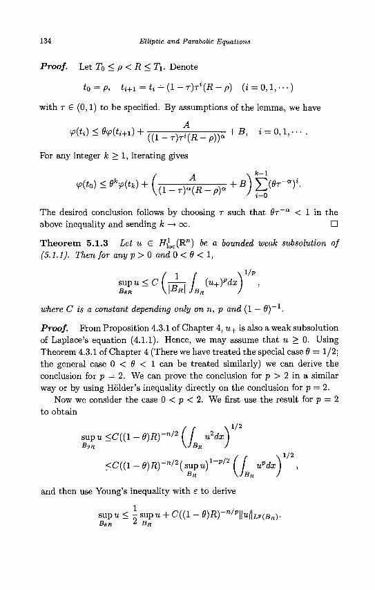
134 Elliptic and Parabolic Equations
Proof. LetT0<p<R<T1. Denote
to = p, ti+1=U + 0--T)Ti(R-P) (t = 0 , l , " - )
with r G (0,1) to be specified. By assumptions of the lemma, we have
^)<Wti+i)+{{1_T)Ti{R_p))a+B, i = 0,l, . . . .
For any integer k > 1, iterating gives
rtto) < *<p{tk) + ({1_T)aA
{R_p)a+B) | > - . ) « .
The desired conclusion follows by choosing r such that Qr~a < 1 in the above inequality and sending k —> oo. •
Theorem 5.1.3 Let u G Hioc(M.n) be a bounded weak subsolution of (5.1.1). Then for any p > 0 and 0 < 6 < 1,
s u p u ^ c f - z j - r / (u+)pdx) Ben Vl-Dfll VBH /
1/p
- 1 where C is a constant depending only on n, p and {1 — 0)
Proof. From Proposition 4.3.1 of Chapter 4, u+ is also a weak subsolution of Laplace's equation (4.1.1). Hence, we may assume that u > 0. Using Theorem 4.3.1 of Chapter 4 (There we have treated the special case 6 = 1/2; the general case 0 < 9 < 1 can be treated similarly) we can derive the conclusion for p = 2. We can prove the conclusion for p > 2 in a similar way or by using Holder's inequality directly on the conclusion for p = 2.
Now we consider the case 0 < p < 2. We first use the result for p = 2 to obtain
supu <C((1 - 6)R)-n'2 ( f u2dx\ Bert \JBR J
O r \1//2
vPdx) , BR J
and then use Young's inequality with e to derive
supw < \ supu + C((l - 9)R)-n/"\\u\\LP{BR). BBR l BR
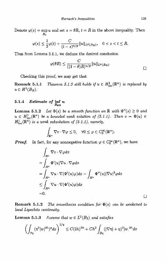
Harnack's Inequalities 135
Denote (f(s) = sup u and set s — 6R, t = R in the above inequality. Then B,
1 C V(») < gVW + ( t_8)n/pllUH^(gi»)' 0 < S < i < i?.
Thus from Lemma 5.1.1, we deduce the desired conclusion
Checking this proof, we may get that
Remark 5.1.1 Theorem 5.1.3 still holds if u G Hioc(Rn) is replaced by
5.1.4 Estimate of inf it Ben
Lemma 5.1.2 Let 3>(s) be a smooth function on R with $"(s) > 0 and u G Hloc(R
n) be a bounded weak solution of (5.1.1). Then v = $(u) G Hyoc(R
n) is a weak subsolution of (5.1.1), namely,
J Ju
Vu • V</> < 0, VO < y> G C^(Rn).
Proof. In fact, for any nonnegative function ip G Co°(Rn), we have
/ Vv • Vipdx JRn
= / $'(u)Vu • V(fdx JR*
= [ Vu-V(&{u)<p)dx- f &'(v)\Vu\2<pdx JRn JRn
; / Vu • V{$'(u)<p)dx JR"
<
=0. a
Remark 5.1.2 The smoothness condition for $(s) can be weakened to local Lipschitz continuity.
Lemma 5.1.3 Assume that w G L2{B2) and satisfies
( f (v2\w\2h)"dx) < C(2h)2h + Ch2 [ (|VT7| + r])2\w\2hdx \JB2 J JB2
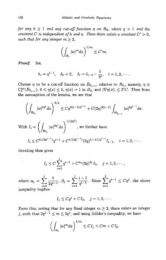
136 Elliptic and Parabolic Equations
for any h > 1 and any cut-off function r] on Bi, where q > 1 and the constant C is independent of h and r\. Then there exists a constant C > 0, such that for any integer m>2,
\w\mdx) < Cm.
Proof. Set
hi = qi~1, S0 = 2, S i ^ S ^ - y , i = 1,2, ••• .
Choose T) to be a cut-off function on Bsi_1, relative to Bst, namely, 77 G C ^ C ^ i - i ) . 0 < r){x) < 1, »j(x) = 1 in BSi and |V??(x)| < 2*C. Then from the assumption of the lemma, we see that
(L 1/9
^dx J < Cq^-W-1 + C{2q)W-V f {w^dx.
\ l/(2<?*)
With It= [ I \w\Zq'dx , we further have
7.<cl/(2^-)gi-i+ci/(29-1)(29)(i-i)/9i-1
/._1) i = i , 2 ) . . . .
Iterating then gives
Ij < C J ] g*"1 + CQ ' (29)ft Jo, j = 1,2, • • • , i = l
J 1 J' i — 1 * where Oj = 5 3 o »_i > &' = 5 3 ;- i • Since 5 ^ ^ _ 1 - ^q^, the above
i = l 9 i = l 9 i = l
inequality implies
Ij^Cqi+CIo, j = 1,2, • • - .
From this, noting that for any fixed integer m > 2, there exists an integer j , such that 2qi~1 <m< 2qj, and using Holder's inequality, we have
l /m
< CIj <Cm + CI0.
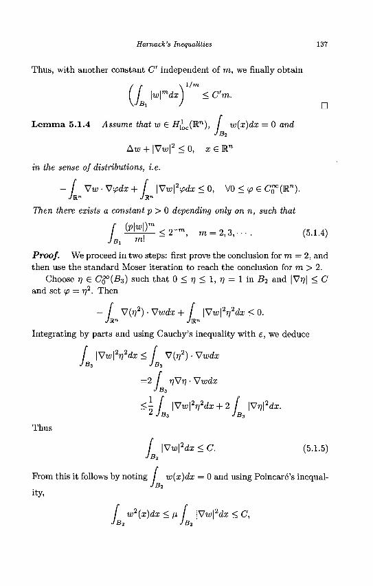
Harnack's Inequalities 137
Thus, with another constant C independent of m, we finally obtain
\w\mdx < Cm. B1 J D
5.1.4 Assume that w € H^c(Rn), / w(x)dx = 0 and
JBi Lemma
Aw + \Vw\2 < 0, x e W
in the sense of distributions, i. e.
-f Vw-Vipdx+ J \Vw\2<pdx<0, V0<<peCZ°(Rn).
Then there exists a constant p > 0 depending only on n, such that
r (P\w\y JBi m\
<2~m, m = 2 ,3 , - - - . (5.1.4)
Proof. We proceed in two steps: first prove the conclusion for m = 2, and then use the standard Moser iteration to reach the conclusion for m > 2.
Choose ri G C$°(B3) such that 0 < r) < 1, 77 = 1 in B2 and |Vr7| < C and set <p = rj1. Then
- / V(T?2) • Vwdx + / \Vw\2n2dx < 0.
Integrating by parts and using Cauchy's inequality with e, we deduce
/ \Vw\2r)2dx < / V(T72) • Vwdx JB3 JB3
=2 / 77V77 • Vwdx JB3
<- I \Vw\2n2dx + 2 I \Vrj\2dx. 2 JB3 JB3
Thus
/ \Vw\2dx<C. (5.1.5) JBi
Prom this it follows by noting / w(x)dx = 0 and using Poincare's inequal-JB2
ity,
/ w2(x)dx <n \Vw\2dx < C, JB2 JBo
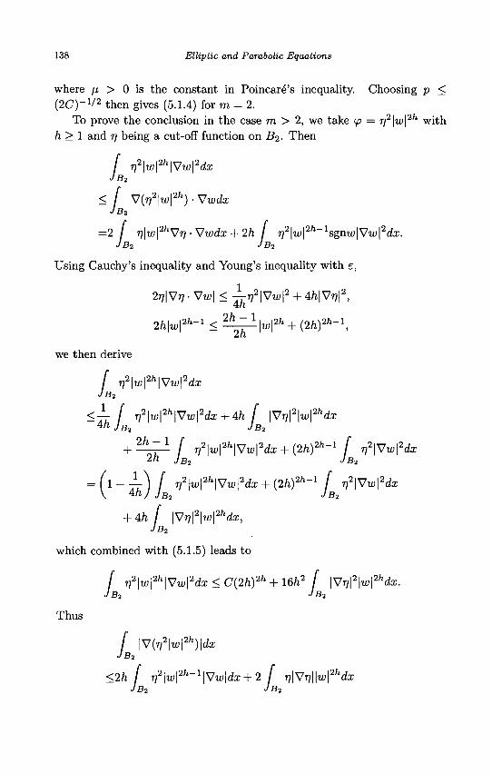
138 Elliptic and Parabolic Equations
where fi > 0 is the constant in Poincare's inequality. Choosing p < (2C)- 1 / 2 then gives (5.1.4) for m = 2.
To prove the conclusion in the case m > 2, we take tp = rj2\w\2h with ft > 1 and 77 being a cut-off function on B^. Then
/ ri2\w\2h\Vw\2dx JB2
< [ V{r?\w\2h) • Vwdx JB2
= 2 / r)\w\2hVrj • Wwdx + 2 f t / 772|w|2/l_1sgni(;|Viy|2dx. J B2 J Bo 1B2 J B2
Using Cauchy's inequality and Young's inequality with e,
277IV7? • Ww\ < —r]2\Vw\2 + 4/i|V7y|2, An
2h\w\2h-1 < ^ ^ H 2 h + {2h)2h~\
we then derive
/ ri2\w\2h\Vw\2dx JB2
< \ [ r)2\w\2h\Vw\2dx + 4h f \Vr)\2\w\2hdx 4ft JB2 JB2
+ : ^ L Z ! f r,2\w\2h\Vw\2dx + (2h)2h~1 f rP\Vv,\2dx 2ft JB2 JB2
= (1~ih) [ V2\w\2h\Vw\2dx + (2h)2h~l f V2\Vw\2dx
+ 4h f \Vr)\2\w\2hdx, JB2
which combined with (5.1.5) leads to
/ r)2\w\2h\Vw\2dx < C(2h)2h + 16h2 f |Vr7 | 2 |u ; | 2^. JB2 JB2
Thus
/ \V(V2\w\2h)\dx
JB2
<2h f rt2\w\2h-1\Vw\dx + 2 f r]\Vri\\w\2hdx
JB2 JB2
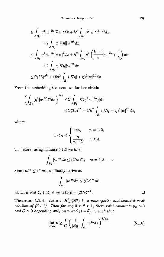
Hamack's Inequalities 139
<[ V2\w\2h\Vw\2dx + h2 f rfH^-^d
+ 2 1 r]\Vr]\\w\2hdx JB2
< f r,2\w\2h\Vw\2dx + h2 f 7 ? 2 f c
+ 2 [ r,\Vr,\\ JBn
h—1, .o/. 1 , , w\2h + -)dx
w\2hdx >B2
\2h , i « 2 <C(2h)2h + 16h2 f (\Vr,\+r,)2\w\2hdx. JB2
Prom the embedding theorem, we further obtain
1/9 f {ri2\w\2h)qdx) <C f \V(r)2\w\2h)\dx
J B2 / J B2
<C{2h)2h + Ch2 f (\Vr]\+r,)2\w\2hdx, JBn.
where
IB2
+00, n = 1,2,
n n > 3.
1 <q < <
. n - 2 '
Therefore, using Lemma 5.1.3 we infer
/ \w\mdx < (Cm)m, m = 2,3
Since m m < emm!, we finally arrive at
/ \w\mdx < (Ce)mm\, JBx
which is just (5.1.4), if we take p = (2Ce)_1 . • Theorem 5.1.4 Let u G Hloc(M.n) be a nonnegative and bounded weak solution of (5.1.1). Then for any 0 < 6 < 1, there exist constants po > 0 and C > 0 depending only on n and (1 — 6)"1, such that
inf u > ^ f T^-T / up°dx) Ben C\\BR\JBR J
\ 1/Po
(5.1.6)
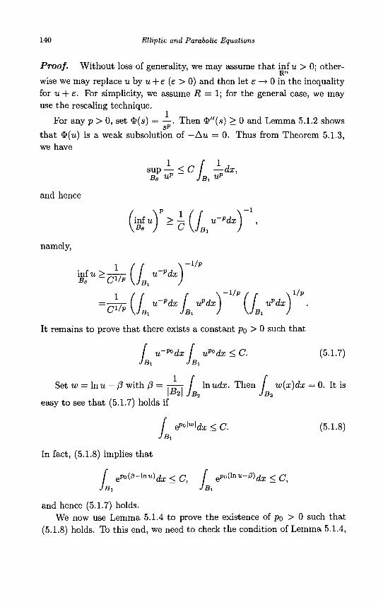
140 Elliptic and Parabolic Equations
Proof. Without loss of generality, we may assume that inf u > 0; other-
wise we may replace u by u + e (e > 0) and then let e —> 0 in the inequality for u + e. For simplicity, we assume R = 1; for the general case, we may use the rescaling technique.
For any p > 0, set $(s) = —. Then $"(s) > 0 and Lemma 5.1.2 shows that $(u) is a weak subsolution of —An = 0. Thus from Theorem 5.1.3, we have
—dx, UP
L - l
u ~pdx
and hence
namely,
inf u Be
1
1
~CXIP
sup —<U Be U" JB
(¥•)'**(/.
/ f \ - I / P
(V""")
=<k(Lu-"*-Is*)'1' \Lu,ixT'• It remains to prove that there exists a constant po > 0 such that
u-podx f upodx < C. (5.1.7) / u-podx J JBi JB1
Set w = lnu — j3 with (3 = -—- / \nudx. Then / u;(a;)(ix = 0. It is
e^i^ldx < C. (5.1.8)
IB2
easy to see that (5.1.7) holds if
JB, IB!
In fact, (5.1.8) implies that
f epo{0-lnu)dx < C j /" epo(lnu-/3) r f 2 . < C ]
and hence (5.1.7) holds. We now use Lemma 5.1.4 to prove the existence of p0 > 0 such that
(5.1.8) holds. To this end, we need to check the condition of Lemma 5.1.4,
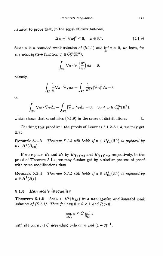
Harnack's Inequalities 141
namely, to prove that, in the sense of distributions,
Aw + \Vw\2 < 0, xeW1. (5.1.9)
Since u is a bounded weak solution of (5.1.1) and inf u > 0, we have, for R"
any nonnegative function y> S Co°(R"),
/ Vu • V ( - ) dx = 0,
namely,
/ - V u • Vv?cta - / —y>|Vu|2d:r = 0
or / VwVipdx- j |Vu/|Vfa: = 0, V0 < <p S CS°(Rn),
,/R" 7R"
which shows that w satisfies (5.1.9) in the sense of distributions. •
Checking this proof and the proofs of Lemmas 5.1.2-5.1.4, we may get that
Remark 5.1.3 Theorem 5.1.4 still holds if u G Hloc(Rn) is replaced by
ueH\B3R).
If we replace B\ and f?2 by B^g+iy2 and -B(0+3)/4, respectively, in the proof of Theorem 5.1.4, we may further get by a similar process of proof with some modifications that
R e m a r k 5.1.4 Theorem 5.1-4 still holds if u G H*oc(M.n) is replaced by u G H\BR).
5.1.5 Harnack's inequality
Theorem 5.1.5 Let u € H1{B3R) be a nonnegative and bounded weak solution of (5.1.1). Then for any 0 < 9 < 1 and R > 0,
sup u < C inf u BBR
B«H
with the constant C depending only on n and (1 — 0 ) - 1 .
142 Elliptic and Parabolic Equations
Proof. From Theorem 5.1.3 and Remark 5.1.1, for any p > 0,
SUP U < C I -j-jr-r / UPdx ) Ben \\BR\ JBR J
On the other hand, from Theorem 5.1.4 and Remark 5.1.3, there exists a constant po > 0, such that
W*h{ikL'f"*y Combining these two inequalities derives the desired conclusion. •
Furthermore, the condition u G H1(B3R) in Theorem 5.1.5 may be replaced by u G H1{BR), according to Remark 5.1.4 or by the finite covering theorem. More general, we have
Theo rem 5.1.6 Let fi C W1 he a domain and u G Hl{Q) he a nonnega-tive and bounded weak solution of (5.1.1). Then for any bounded suhdomain Q' cc fi,
supu<Cinfu (5.1.10)
n> fi'
with the constant C depending only on n, fi' and fi.
Proof. Fix
0< i?< Jdist(fi',<9fi).
For any x G fi , from Theorem 5.1.5, there exists a constant C depending only on n such that
sup u < C inf u. (5.1.11) BR(X) B H W
Choose xx,x2 G fi so that
sup u = supu, inf u = infu. (5.1.12) BR(x*) fi' BR(x2) H'
Let r C fi be a closed arc joining a;1 and x2. By virtue of the finite covering theorem, T can be covered by a finite number N (depending only on fi' and fi) of balls of radius R. Applying the estimate (5.1.11) in each ball and
Harnack's Inequalities 143
BR{X1)I BR{X2), respectively, and combining the resulting inequalities, we
obtain
sup u<CN+2 inf u.
Then, (5.1.10) follows from this and (5.1.12). •
5.1.6 Holder's estimate
The following auxiliary lemma is useful in proving the Holder continuity of solutions.
Lemma 5.1.5 Let w(R) be a nonnegative and nondecreasing function on [0, RQ\. If there exist 6, n £ (0,1), 7 £ (0,1] and K > 0, such that
UJ{6R) < T]UJ(R) + KRt, 0<R<R0, (5.1.13)
then there exist constants a € (0,7) and C > 0 depending only on 6, i), 7, such that
u(R)<c(^-) [u(Ro) + KI%], 0<R<R0. (5.1.14)
Proof. We may take 77 so close to 1 that 0_7?7 > 1 and (5.1.13) still holds. Let Ro € (6Ro,Ro] and denote
RS=6SR0, s = 0 , l , 2 , - - - .
Then, from (5.1.13) we have
u(Rs+1)<r,Lj(Rs) + KiFs, s = 0 , l , 2 , - - - .
Iterating gives, for s = 0,1,2, • • • ,
?7
Ls—m—1 « A ) <vs"(Ro) + Yl Kr>mRl
m=0
<r,3u(Ro) + KRp^-V J2 (e^rj)7
m = 0
^ui^ + KRp^-^^^
144 Elliptic and Parabolic Equations
# - 7 Rs
where C = — . Since s = log^ -=4, we have 0 JV ~ 1 Ro
w(Ra)<(5A [w{Ro) + CKRl]
-C[lt) M ^ + ^ o ] , s = 0,l,2,--.,
where a = r—- G (0,7). Let .ffo vary over (9R0,Ro\. Then fta (s = hit)
0,1,2, • • •) varies over (0, RQ\. Thus we can obtain (5.1.14) from the above inequality. •
Theorem 5.1.7 Let ! ! c R " be a domain and u G i71(fi) be a bounded weak solution of (5.1.1). Then for any bounded subdomain il' CC fl, there exists a constant a G (0,1) such that
[u]a;{V < C,
where C is a constant depending only on n, il' and Q.
Proof. For any fixed x° e ft' and 0 < R < -dist(fi ', dfl), denote o
m(R) = inf u, M(R) = supu, B « BR
where BR = BR(x°). Let
v(x) = u{x) —m(R), w(x) = M(R) -u(x).
Then v,w G H1(B3R) are nonnegative and bounded and —Av — —Aw = 0 in B3R in the sense of distributions. Using Harnack's inequality to v and w gives
sup v < C inf v, sup w < C inf w, BR/2
B « / 2 B R / 2 B « / 2
namely,
M{R/2)-m{R) < C[m{R/2)-m{R)\, M{R)-m(R/2) < C[M{R)-M{R/2)
We may assume C > 1; otherwise we replace C by C + 1. From the above two inequalities, we see that
M(R/2) - m(R/2) < ^±[M(R) - m{R)\.
Harnack's Inequalities 145
C — 1 Denote f(R) = M(i?) — m(R), 77 = ——-. Then f(R) is nonnegative and
G + 1 nondecreasing and satisfies
/GR/2) < r,f(R).
By the iteration lemma (Lemma 5.1.5), there exists a £ (0,1), such that
f(R) < CRa,
namely,
Ma;BR(x°) < C.
The conclusion of the theorem can then be completed by an easy covering argument. •
5.2 Harnack's Inequalities for Solutions of the Homogeneous Heat Equation
In §5.1, we have proved that for nonnegative and bounded weak solution u e H^c(R
n) of (5.1.1), there holds
sup u < C(n, 9) inf u, V0 e (0,1). Ben B<>R
A natural question is that for the homogeneous heat equation
— - Au = 0, (x, t ) £ f x R+ (5.2.1)
whether the analogous inequality
sup u < C(n, 9) inf u, V6> € (0,1) (5.2.2) QeR Go*
holds? The following example shows that the answer is negative.
Example 5.2.1 The equation ut — uxx = 0 has a nonnegative and bounded solution on (—R,R) x [0,i?2],
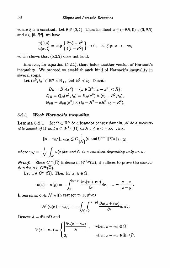
146 Elliptic and Parabolic Equations
where £ is a constant. Let 9 G (0,1). Then for fixed x G (-OR, 0) U (0,9R) and* G [0,.R2], we have
u(0,t) f 2x£ + x2 I = eXP\4(t + R2)) ' a-55 £ s S n x ^ - ° ° > u(cc,i)
which shows that (5.2.2) does not hold.
However, for equation (5.2.1), there holds another version of Harnack's inequality. We proceed to establish such kind of Harnack's inequality in several steps.
Let (x°,t0) G Rn x R+, and R2 <t0. Denote
BR = BR(x°) = {xe Rn; \x - x°\ < R},
QR = QR(x°,t0) = BR(x°) x (t0 - R2,t0),
QeR = BeR(x°) x (to - R2 - OR2, t0 - R2).
5.2.1 Weak Harnack's inequality
Lemma 5.2.1 Let 0 C R" be a bounded convex domain, H be a measurable subset o/fi and u G W1'P(Q) with 1 < p < +oo. Then
\\u - u/s\\LP{n) < C-^j-(diamn)"+1||Vu||Lp(f2),
where uyy = -rrTi / u(x)dx and C is a constant depending only on n. =w\Lu{
Proof. Since C°°(Q) is dense in W1,P(Q), it suffices to prove the conclusion for u G C°°(Ti).
Let u G C°°(T7). Then for x,y&9,,
u(x) - u(y) = - / Jo
x v' du(x + ruj) , y — x dr. OJ — ,0 dr \x-y
Integrating over Af with respect to y, gives
\M\(u(x) - UM) = - J J ^ drdy.
Denote d = diamfi and
du(x + rw)
V(x + rw) = when x + ru> G Cl,
dr
0, when x + rw € R n \Q .
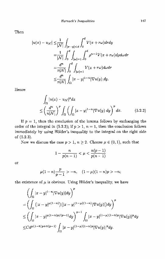
Harnack's Inequalities 147
Then
\u(x) -utf\ <Yj-7: I / V(x + roj)drdy \-N\ J\x-y\<dJo
=JTn I f I pn-lV{x + ru)dpdujdr \-N\ Jo J\u\=iJo
J0 J\ui\ = l
dn
nW\ JO j \ u \ x + rw)dwdr
^w\L]x-yll~n]Vu{y)ldy-Hence
/ \u(x
Jn ) — u/s\pdx
4^"L(ilx-yll"'Wy)]dv)'di- (5-2-3) If p = 1, then the conclusion of the lemma follows by exchanging the
order of the integral in (5.2.3); if p > 1, n = 1, then the conclusion follows immediately by using Holder's inequality to the integral on the right side of (5.2.3).
Now we discuss the case p > 1, n > 2. Choose /x € (0,1), such that
1 _ ^ _ < / x < ^ - 1 ) p(n — 1) p(n — 1)
or P /i(l — n) > — n, (1 — /i)(l — n)p > — n;
p-1
the existence of /x is obvious. Using Holder's inequality, we have
= (_£ (\x - yr{1-n)) (\x - j/|<1-"><1-n>|Vu(j/)|)dj/)P
< ( [ \x - ylM-nWto-Vdy) f \x- y\{l-^){1-n)p\Vu{y)\pdy \Jn J Jn
<CdM(l-n)p+n(p-l) J |a; _ y|<1-^(1-")P|VM(l/) |pdj/ . JQ.
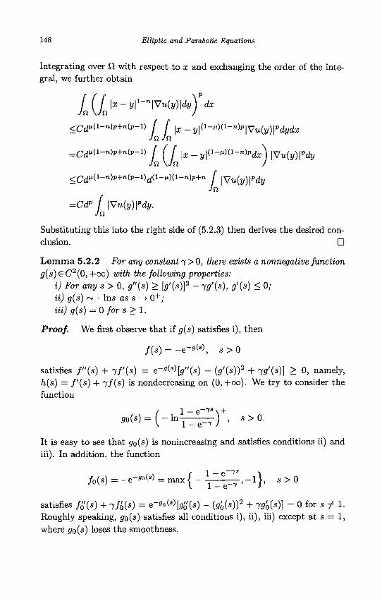
148 Elliptic and Parabolic Equations
Integrating over fi with respect to x and exchanging the order of the integral, we further obtain
jf Qjjz-yMVuMldi/Yda;
< C d M(l-n) P +n(p- l ) J f \x - y\Q-lM-n)P\S7u(y)\Pdydx JnJn
=C-dM(l-n)lH-n(p-l) f f f ^ _ y^-Ml-nfrfa} |Vu(y)|"dj/
<CdM(i-n)p+n(P-i)d(i-M)(i-n)P+n / \Vu(y)\pdy Jn
=C<F [ \Vu(y)fdy.
Substituting this into the right side of (5.2.3) then derives the desired conclusion. •
Lemma 5.2.2 For any constant 7 > 0, there exists a nonnegative function j ( s ) s C 2 ( 0 , +00) with the following properties:
i) For any s > 0, g"(s) > [g'(s)}2 - yg'(s), g'(s) < 0; ii) g(s) ~ —Ins as s —> 0 + ; Hi) g(s) = 0 for s > 1.
Proof. We first observe that if g(s) satisfies i), then
/ (s) = - e - s ( s \ s > 0
satisfies f"{s) + jf'(s) = e-^[g"(s) - (g'(s))2 + 7</(s)] > 0, namely, h(s) = f'(s) + 7/(s) is nondecreasing on (0, +00). We try to consider the function
(to(s)= ( - I n — — J , s > 0 .
It is easy to see that go{s) is nonincreasing and satisfies conditions ii) and iii). In addition, the function
-7s - 1_e-T>-1}> S > 0
satisfies fS(s) + jf^(s) = e"*. W[0»(a) - (g>0(s))* + ig'0(s)} = 0 for s ± 1. Roughly speaking, go(s) satisfies all conditions i), ii), iii) except at s = 1, where go(s) loses the smoothness.
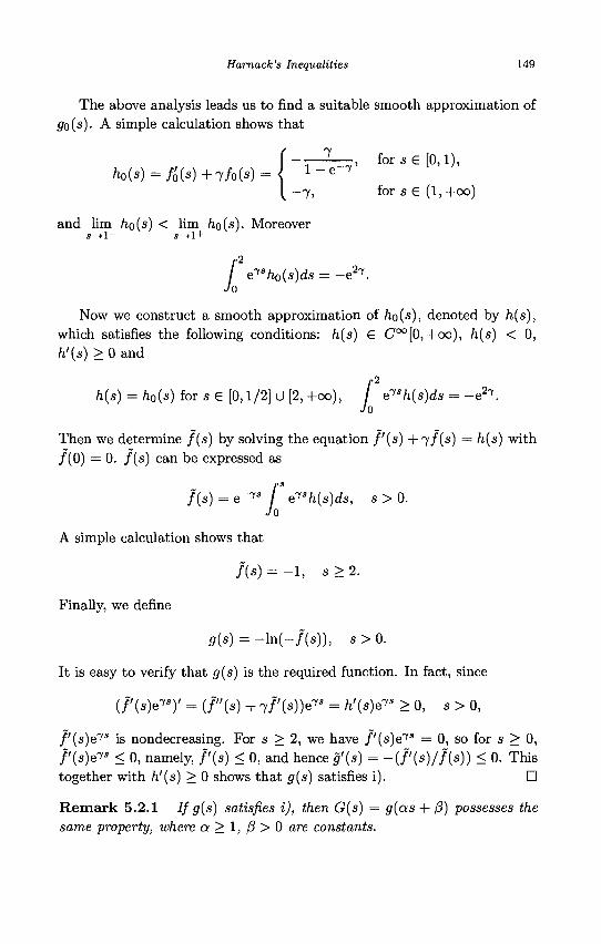
Hamack's Inequalities 149
The above analysis leads us to find a suitable smooth approximation of go(s)- A simple calculation shows that
~-—, for s € [0,1), M * ) = /o(*)+7/o(s) = < 1 - e " 7
—7, for s G (l ,+oo)
and lim ho(s) < lim ho{s). Moreover s—+l~ a—>1 +
f JO
e^sho(s)ds = - e 2 7 .
Now we construct a smooth approximation of ho(s), denoted by h(s), which satisfies the following conditions: h(s) G C°°[0, +00), h(s) < 0, h'{s) > 0 and
h{s) = h0(s) for s G [0,1/2] U [2, +00), / ersh(s)d Jo
s = -e2\
Then we determine f(s) by solving the equation f'(s) + jf(s) = h(s) with /(0) = 0. f(s) can be expressed as
/ (s ) = e - 7 * / e~<sh(s)ds, s > 0. /o
A simple calculation shows that
f(s) = - 1 , s > 2.
Finally, we define
g(s) = - l n ( - / » ) , 5 > 0 .
It is easy to verify that g(s) is the required function. In fact, since
(f'(s)e^)' = (f"(s) + ff'(s))eT = h'W > 0, s > 0,
f'(s)e'ys is nondecreasing. For s > 2, we have f'(s)ey3 = 0, so for s > 0, /'(s)eTs < 0, namely, f'(s) < 0, and hence g'(s) = - ( / ' ( s ) / / ( s ) ) < 0. This together with ft'(s) > 0 shows that g(s) satisfies i). •
R e m a r k 5.2.1 If g(s) satisfies i), then G(s) = g(as + (3) possesses the same property, where a > 1, 0 > 0 are constants.
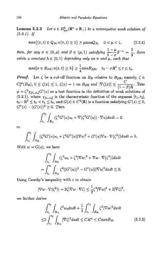
150 Elliptic and Parabolic Equations
Lemma 5.2.3 Let u £ H{oc(Rn x R+) be a nonnegative weak solution of
(5.2.1). If
mes{(x, t) eQR-,u(x,t) >1} > fimesQR, 0 < / i < 1, (5.2.4)
1 — u 2 then, for any a £ (0, (J,) and f3 £ (/i, 1) satisfying - 0 n = -, there
1 — cr 3 exists a constant h £ (0,1) depending only on n and /J,, such that
mes{a; £ BpR; u(x, t) >h} > -mesBpR, to — o-R2 <t<t0.
Proof. Let £ be a cut-off function on BR relative to BpR, namely, C £
CS°(BR), 0 < C(a?) < 1, C(z) = 1 on 5 ^ and |V<(a;)| < ( 1 ° ) R - Take
yj = C2X[tj,t2]^'(u) as a tes* function in the definition of weak solutions of (5.2.1), where X[ti,t2] *s * n e characteristic function of the segment [ii,^]) t0-R
2 < h < t2 < t0, and G(s) £ C2(R) is a function satisfying G'(s) < 0, G"(s) - (G'(s))2 > 0. Then
[ 2 / (C2G'(u)ut + V(C2G'(u)) • Vu)dxdt = 0 Jti JBR
or
f2 j {C2G'(u)ut + {2G"(u)\Vu\2 + G'{u)Vu-V(C2))dxdt = 0. Jti JBR
With w = G(u), we have
2wt + C2|Vu;|2 + Vu> • \/{C,2))dxdt
= f2 I C2[(G'(u))2 - G"(u)]\Vu\2dxdt < 0. Jt! JBR
Using Cauchy's inequality with e to obtain
|V«> • V(C2)| = 2C|VW • VC| < \<?\Vw? + 2|VC|2,
we further derive
I \ C2wtdxdt+- / C2\Vw\2dxdt Jti JBR 2 Jtl JBR
\V<:\2dxdt < CRn < CmesBR. (5.2.5)
Jt! JBR
Jn JBR
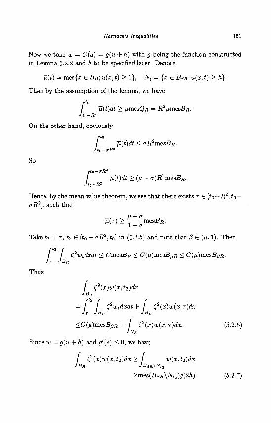
Harnack's Inequalities 151
Now we take w = G(u) = g(u + h) with g being the function constructed in Lemma 5.2.2 and h to be specified later. Denote
jET(t) = mes{x G BR-,u(x,t) > 1}, JVt = {x e BpR-,u(x,t) > h}.
Then by the assumption of the lemma, we have
/imesQfi = i?2jUmesB/j. /•to
/ -p{t)dt > Jto-R2 >to-
On the other hand, obviously
/•to
/ ~p{t)dt < aR2mesBF
So
rto-<rR2 /•to-
Jto-fi(t)dt > (/i — a)R mesBR.
R2
Hence, by the mean value theorem, we see that there exists r G [to — R2, to — CTR2}, such that
/X(T) > mes.BR. l — cr
Take h =r,t2€ [t0 - crR2,t0] in (5.2.5) and note that /3 G (fi, 1). Then
(,2wtdxdt < CmesBjt < C(/x)mesJBMij < C(fi)mesBpR. n JT JB,
'BR
Thus
(2(x)w(x,t2)dx BR
= / C,2wtdxdt + / C,2{x)w(x,T)dx
<C(hi)mesB0R + / C2{x)w(x,r)dx. (5.2.6) JBR I BR
Since w — g(u + h) and g'(s) < 0, we have
/ C,2(x)w(x,t2)dx > / w(x,t2)dx •IBR JB0R\Nt2
>mes{B0R\Nt2)g(2h)- (5-2.7)
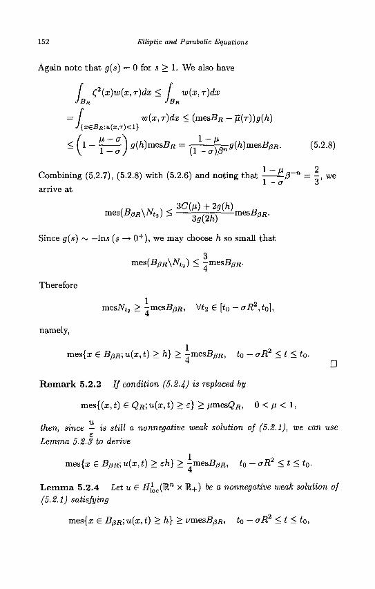
152 Elliptic and Parabolic Equations
Again note that g(s) = 0 for s > 1. We also have
/ C,2(x)w{x,r)dx < I w(x,r)dx JBR JBR
— / w(x,r)dx < (mesBR — Jl(T))g(h) J{X€BR;U(X,T)<1}
^ f1 ~ Y ~ ) 9(h)mesBR = -L=J~g(h)mesBm. (5.2.8)
Combining (5.2.7), (5.2.8) with (5.2.6) and noting that — — / 3 ~ n = - , we 1 — a 3
arrive at ,„ S.T s ^ 3C(n) + 2g(h)
m e s ^ . j A A U < 3 ( 2 M mesBW-
Since g(s) ~ —Ins (s —> 0+) , we may choose h so small that
3 mes(B/3/i\Aft2) < -mesB^fi.
Therefore
mes7Vt2 > -mesBpR, Vt2 € [<0 - o-R2,t0],
a
namely,
mes{x € Bj3R; u(x, t) > h} > -mesBpn, to - eR2 <t<t0.
Remark 5.2.2 / / condition (5.2.4) is replaced by
mes{(x,t) G QR;u(x,t) > e} > /xmesQ/j, 0 < fj, < 1,
then, since — is still a nonnegative weak solution of (5.2.1), we can use e
Lemma 5.2.3 to derive
mes{z G BpR; u(x, t) > eh} > - m e s S ^ , t0 - o-R2 <t<t0. 4
Ton *j 'locV Lemma 5.2.4 Let u G H^oc(R
n x R + ) be a nonnegative weak solution of (5.2.1) satisfying
mes{z £ BpR; u(x, t) > h} > ismesBpR, t0 - crR2 <t <t0,
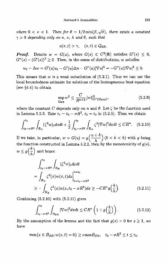
Harnack's Inequalities 153
where 0 < v < 1. Then for 6 = l/2min(/3, -</&), there exists a constant 7 > 0 depending only on n, v, h and 9, such that
u(x,t)>j, (x,t)£QeR-
Proof. Denote w = G(u), where G(s) € C2(E) satisfies G'(s) < 0, G"(s) — (G'(s))2 > 0. Then, in the sense of distributions, w satisfies
wt - Aw = G'(u)ut - G'(u)Au - G"(u)\Vu\2 = -G"{u)\Vu\2 < 0.
This means that w is a weak subsolution of (5.2.1). Thus we can use the local boundedness estimate for solutions of the homogeneous heat equation (see §4.4) to obtain
S u p W2 < - ^ H H 2 ( 0 2 e R ) , (5-2.9)
where the constant C depends only on n and 6. Let £ be the function used in Lemma 5.2.3. Take t\ = to — CTR2, ti = to in (5.2.5). Then we obtain
/ / {(?w)tdxdt + \ [° [ <;2\Vw\2dxdt<CRn. (5.2.10) Jto-oR? JBR 2 Jtg-aR2 JBR
If we take, in particular, w = G(u) = g(—-—J (0 < fc < h) with g being
the function constructed in Lemma 5.2.2, then by the monotonicity of g(s),
w < g (— J and hence
/ / Jto-oR2 JBR
(C w)tdxdt
t=t0
t=to-<rR2 £2(x)w(x,t)dx
>- f <:2(x)w{x,t0-aR2)dx>-CRng(^). (5.2.11) IBR
Combining (5.2.10) with (5.2.11) gives
rto
[° f \S7w\2dxdt<CRn(l+g(^)\ (5.2.12) Jto-vRiJBpR \ ^hJ J
By the assumption of the lemma and the fact that g(s) = 0 for s > 1, we have
mes{a: 6 BpR;w(x,t) = 0} > vmesBpn, to — crR2 <t<t0.
154 Elliptic and Parabolic Equations
Using Lemma 5.2.1 with Q = BpR and N = {x £ BpR; w(x, t) = 0}, we see that, for any to — aR2 <t<to,
f w2(x,t)dx <C^f]" [ \Vw(x,t)\2dx JB0R \M I JB0R
< C ( W " + 2 J \Vw{X:t)\2dx I-O/JHI JB0R
<CR2 f \Vw{x,t)\2dx. J BgR
Prom (5.2.12), we further obtain
/•to r /-to r / / w2(x,t)dxdt<CR2 / \Vw\2dxdt
Jto-aR2 JBgR Jto-crR2 JB0R
< C R » « ( i + 9 ( i ) ) .
Combining this with (5.2.9) yields
supi*2 < -£&\MIHQMR) < C ( l + g(±)) . (5.2.13)
Choosing 7 so small that 27 < h and
2
we must have u > 7 on Qefi- Suppose, to the contrary, there exists (x, i) € QOR, such that u(x,i) < 7. Then from (5.2.13), we would have
which contradicts (5.2.14). D
Prom Remark 5.2.2 and Lemma 5.2.4, we obtain
Theorem 5.2.1 (Weak Harnack's Inequality) Assume that u £ 77[QC(R™ x R_|_) is a nonnegative weak solution of (5.2.1) and for some constants e > 0 and fi £ (0,1),
mes{(a:,£) £ QR\u(x,t) > e} > ^imesQR.
Harnack's Inequalities 155
Then there exist a constant 6 £ (0,1/2) depending only on n and fi and a constant 7 > 0 depending only on n, /x, e and 0, such that
u ( x , £ ) > 7 , V(x,t)€Q6R.
5.2.2 Holder's estimate
Applying the weak Harnack's inequality, we can establish interior Holder's estimate for solutions of the homogeneous heat equation.
Lemma 5.2.5 Let u e i?1(Qfl0) be a bounded weak solution of (5.2.1) in QnQ. Then there exist constants 6 € (0,1/2) and a € (0,1) depending only on n, such that for any 0 < R < RQ/2, either
i) osc u < CR QOR
or ii) osc u < aoscu.
QeR QR
Proof. Denote M = sup u. Without loss of generality, we may assume QR
that ui(R) = osc u = 2M; otherwise we consider v = u — — ( sup u + inf u QR 2 \ Q R QR
instead of u, which is a bounded weak solution of (5.2.1) with
oscw = osc it = 2supv. Q R QR QR
If M < R, then for 6 € (0,1), we have
osc u < osc u — 2M < 2R, QSR QR
which implies i). To prove ii) in case M > R, note that one of the following two cases
must be valid:
mes{(a;,t) € QR,U > 0} > -mesQR
and
mes{(a;,i) € QR, —U > 0} > -mesQj?.
156 Elliptic and Parabolic Equations
U For defmiteness, we assume that the first one is valid. Let u = 1 H . _, M Then u > 0 and
mes{(:r,£) G QR,U > 1} > -mesQ^.
From the weak Harnack's inequality (Theorem 5.2.1), it follows that there exist 6 G (0,1/2) and 0 < 7 < 1, such that
Thus
Hence
u(x , t )>7> (x,t)eQdR.
- M ( l - 7) < u(x, t) < M, (x, t) G Q8R.
ui{6R) = supu - inf u < 2M(l - - ) = acj(R)
7 with a = 1 — —. n
2 Using the iteration lemma (Lemma 5.1.5), we can obtain
Corollary 5.2.1 Let u G i/1(Qfl0) be a bounded weak solution of (5.2.1). Then there exist constants a G (0,1) and C > 0 depending only on n, such that
osc u < G -=— QR \RO
Furthermore, we have
osc u + Ro 9*o
, 0<i?<i?o-
Theorem 5.2.2 Let u G H^^W1 x R + ) be a bounded weak solution of (5.2.1). Then there exists a constant a G (0,1), such that for any QR C QR C M.n x R+,
b4a,QR < C,
where the constant C depends only on n and QR.
5.2.3 Harnack's inequality
Using the weak Harnack's inequality (Theorem 5.2.1) and Holder's estimate (Theorem 5.2.2). We can derive the following Harnack's inequality.
Harnack's Inequalities 157
Theorem 5.2.3 Let u G Hloc(Rn x R + ) be a nonnegative and bounded
weak solution of (5.2.1). IfAR2 < to, then there exists a constant 6 € (0,1) depending only on n, such that
sup u < C inf u, eR QSR
where the constant C depends only on n and 6.
Proof. We may assume that R = 1, since in the general case, we can transform the problem to the case R = 1 by rescaling.
Suppose first supu = 1. Prom Theorem 5.2.2, there exist constants Oi
a G (0,1) and C > 0 depending only on n, such that [U]Q,Q2 < C. Since ©i C Q2, there must be constants e > 0 and \x G (0,1) depending only on n but independent of u, such that
mes{(x,t) G Q2\u{x,t) > e} > /xmes<52-
From Theorem 5.2.1, it follows that there exist a constant 9 G (0,1) depending only on n, // and a constant 7 depending only on n, /i, e and 8, such that
u(x,t) > 7, (x,t) G Qe-
Thus
sup u = 1 < — inf u 0! 7 Qe
and the conclusion of the theorem follows with C = —. 7
The case supix = 0 is trivial. For the general case supu > 0, we consider 6 i 0 1
w = u, which is also a nonnegative and bounded weak solution of supw 0 i
(5.2.1) with supw = 1. Thus, from what we have proved, ©i
supw — 1 < Cinf w. 0 i Qo
Multiplying both sides by sup u leads to Qi
sup u < C inf u. © i Qe n
158 Elliptic and Parabolic Equations
Exercises
1. Assume that fi C KB is a bounded domain and u € C(Cl) satisfies the mean value equality, namely, for any y £ft and R > 0,
u(y) = „ , P n _ ! / u(x)ds, nwnRn l JdBR
provided BR(J/ ) C Bji(y) C CI. Prove that u € C2(fi) and satisfies Laplace's equation
- A u = 0, x e Q,
where Bn{y) is the ball in Rn of radius R, centered at y, wn is the measure of the unit ball in Rn .
2. Prove Remarks 5.1.1, 5.1.3 and 5.1.4. 3. Assume that BR is a ball in R" of radius R, f € L°°(BR) and
u G H1 (BR) is a nonnegative and bounded weak solution of
-Au = / , x£ BR.
Set u = u + i?2 | |/| |Loo (BK). Prove that for any 0 < 6 < 1,
sup u < C inf u, BeR
BOR
where C > 0 is a constant depending only on n, (1 — 0 ) _ 1 and ||u||i,«>(BR). 4. Establish the weak Harnack's inequality for solutions of the nonho-
mogeneous heat equation.
Chapter 6
Schauder's Estimates for Linear Elliptic Equations
In this and next chapters, we introduce Schauder's estimates for linear elliptic equations and linear parabolic equations of second order respectively. These estimates will be applied to the existence theory of classical solutions in Chapter 8. In this chapter, Schauder's estimates will be established first for Poisson's equation. To establish Schauder's estimates for such a typical and simple in form equation, one can easily expound the basic idea of the method and catch the essence of the argument. Based on the results obtained for this equation, we finally complete the estimates for general linear elliptic equations.
To establish Schauder's estimates, we will adopt the theory of Cam-panato spaces. By means of such approach, the derivation will be more succinct compared with those based on the potential theory or based on mollification of functions given by Trudinger. In addition, this approach is available not only to linear elliptic equations and systems of second order, but also to equations and systems of higher order.
6.1 Campanato Spaces
Schauder's estimates are a priori estimates on the Holder norms of the derivatives of solutions, which are certain kind of pointwise estimates. It is well-known that in many cases, it is quite difficult to derive pointwise estimates directly from the differential equation considered. However, to derive integral estimates is relatively easy. Thus it is reasonable to ask if there is some approach based on an integral description, instead of the above pointwise estimate. The answer is positive. In this section the Campanato spaces are introduced to describe the integral characteristic of the Holder continuous functions.
159
160 Elliptic and Parabolic Equations
Definition 6.1.1 Let fi C 1 " be a bounded domain. If there exists a constant A, such that for any x &Q and 0 < p < diamfi,
\Qp(x)\ > Apn,
where Clp(x) = Q,nBp(x), then fi is called a domain of (A)-type.
Definition 6.1.2 (Campanato Spaces) For p > 1, p, > 0, the subset of all functions u in LP(Q) satisfying
Mp,wn = SUP \P " \ \u(y) ~ uxJpdy
•en V J£l„(x) i
l/V
J < +00 \ . /oc-r i /
0<p<diamf2
and endowed with the norm
\\u\\Cv.» = \\u\\a>^(n) = [u]p^-ii + ||u||z,p(n)
is called a Campanato space, denoted by £p'M(fi), where
Ux'p = T?nvYT / u^dy-
Note that [ix]p,M;n is a semi-norm rather than a norm, since [u]p>M;n = 0 dose not imply u = 0.
It is easy to verify
Proposition 6.1.1 Cp'^(Q)is a Banach space.
Proposition 6.1.2 (Property of the Mean Value) Let Q C Rn be a domain of (A)-type and u € £p '^(fi). Then for any x € Q and p such that 0 < p < R < diamfi, there holds
K * - «*,p| < c[u]p ,M;n/o-" /pi?M/p ,
where the constant C depends only on A and p.
Proof. For any y £ Op(x), we have
\ux,R - uxJp < 2p-\\ux,R - u(y)\p + \ux<p - u(y)\p).
Integrating over Clp(x) C $IR(X) with respect to y leads to
\tiP{x)\\ux,R - uXyP\p
<2p-x ( [ \ux,R - u(y)\pdy + [ \uXiP - u(y)\pdy) . \JnR(x) Jo.f,(x) J
Schauder's Estimates for Linear Elliptic Equations 161
Hence
Apn\ux,R - uXiP|" < C M ^ ; n ( ^ + pP) < C[u]l^nR»
or
\UZ,R ~ «x,p| < C[u}PMnp-n^R^
with another constant C. D
Theorem 6.1.1 (Integral Characteristic of Holder Continuous Functions) If Q is a domain of (A)-type and n < p, < n + p, then £p,M(f2) = Ca(U) and
Ci[u]a-n < MP,M;n < C2[u)afr,
ix — n where a = and C\, Ci are some positive constants depending only
P on n, A, p, p.
The precise meaning of £"'"(0) = CQ(fi) is that Ca(H) c £ ^ ( 0 ) and for any u G £p , , i(Q), there exists a function u G Ca(Q.) such that u = u a.e. in fi.
Proof. Let u G Ca(fi). Then for any a; G fi, 0 < /o < diamfi and y G fip(x), we have
*(y) - u^l = 1
" \np(x)
<-
Qp(x) (u{y) - u(z))dz
——Y, / \u(y) - u(z)\dz
< Ma-,n / I w - z ^ d z
<M^i / k r d z
-^jf"*"*""** where w„ is the measure of the unit ball in R™. Hence
p-" / |«(y) - Ul,„|*dy < c'Ka;fir-^,(^)l < o w < . n
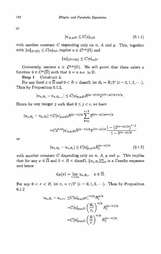
162 Elliptic and Parabolic Equations
Mp,M-,n < C[u]a.}n (6.1.1)
with another constant C depending only on n, A and p. This, together with ||u||z,P(n) < C|u|o;n implies u € £ ^ ( 0 ) and
Ilull£p.c(n) < C|u|a ;n.
Conversely, assume u € Cp'^(il). We will prove that there exists a function u € Ca(fi) such that u = u a.e. in CI.
Step 1 Construct u. For any fixed x € Ti and 0 < R < diamfi, let Ri = R/2i (i = 0,1,2, • • •).
Then by Proposition 6.1.2,
\ux,Ri - uXtRi+1\ < C[u]PlMinie ("-n) /p2 i<n-">/*+"/'\
Hence for any integer j such that 0 < j < i, we have
i - l
r,fl, - « * , * ! < C [ U ] p , w n ^ - n ) / p ^ 2 , : ( " " M ) / p + " / p
i-i —C,1nl'p\t\\ -T>(v--n)/Pni(n-n)/p \ / - o z iujp,M;n/t z 1 _ 2 ( n _ M ) / p
or
Kit , - «*,«, I < C[u)p^nR^'n)/p (6.1.2)
with another constant C depending only on n, A, p and /i. This implies that for any x £ fl and 0 < i? < diamfi, {ux,iJi}i^o ' s a Cauchy sequence and hence
UR(X) = lim u I | f i i , a; G fi.
For any 0 < r < R, let r< = r/2* (i = 0,1,2, • • •). Then by Proposition 6.1.2
K A -Ux.rJ <C[u]P i M ;nrp / p i?f / p
( p \ n / p
7 ) ^-")/p-
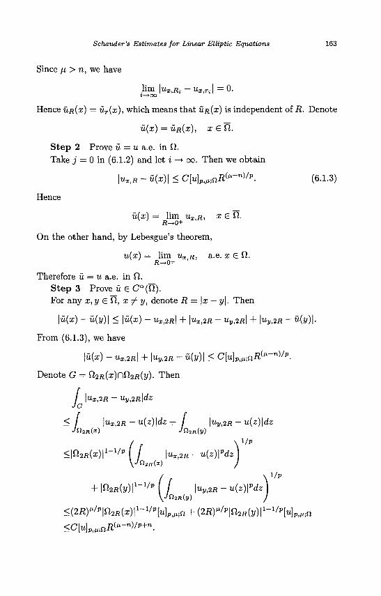
Schauder's Estimates for Linear Elliptic Equations 163
Since \i > n, we have
lim |ux,Ri - Ux,n | = 0. i~+00
Hence UR(X) = ur{x), which means that UR(X) is independent of R. Denote
u(x) = UR{X), I £ ( 1 .
Step 2 Prove u = u a.e. in Cl.
Take j = 0 in (6.1.2) and let i —> 00. Then we obtain
K H - u(x)\ < C[u]p^R{tl-n)/p. (6.1.3)
Hence u(x) = lim ux A, a; £ fi.
ij—0+
On the other hand, by Lebesgue's theorem,
u(x) = lim ux R, a.e. x € fi. fi->0+
Therefore u = u a.e. in Q. Step 3 Prove fi G C a (0 ) . For any x,y £fl, x ^ y, denote R = \x — y\. Then
|u(:r) - u(y)| < \u{x) - UX,2R\ + \UX,2R - uyaR\ + \uy,2R - u{y)\.
From (6.1.3), we have
\u(x) - ux,2R\ + \uy,2R - fife)I < C[u]p,Minii (M-n) /p.
Denote G = f22fi(x)nQ2ij(y). T h e n
/ \Ux,2R - Uy,2R\dz JG
< \ux,2R - u(z)\dz+ / |u„ i 2f l -u(z) |dz v/f!2R(x) Jtl2n.(y)
< | ^ 2 J R ( ^ ) | 1 - 1 / P ( / |u I l 2 R-u(z)|P(fc \JCl2R(x) j
+ |0 2 f l (y) | 1 - 1 / p ( f \uyt2R - u(z)\pdz) \Jn2R(y) )
< ( 2 i ? ) ^ | n 2 f l ( x ) | 1 - 1 / p N P , w f i + {2RylP\£l2R{y)\l-l'P\u]p^n
<C[u}PMaR{il-n)'p+n.
i /p
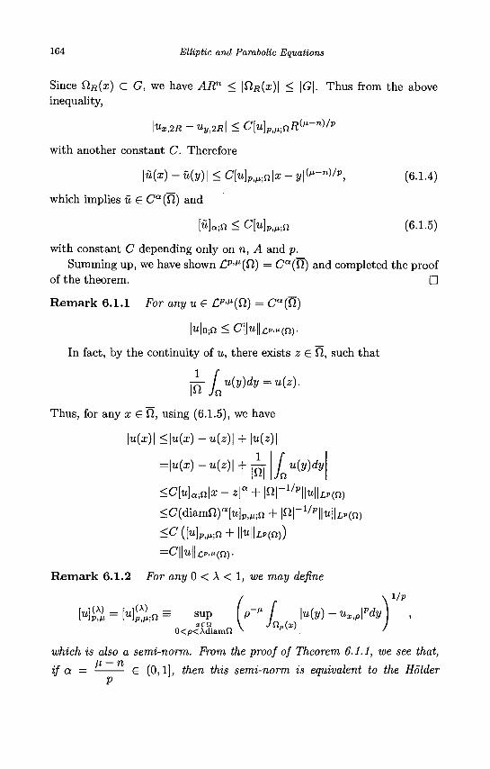
164 Elliptic and Parabolic Equations
Since SlR(x) C G, we have ARn < \SIR(X)\ < \G\. Thus from the above inequality,
\ux,2R - uyt2R\ < C[u}p^nR(,i-n)/p
with another constant C. Therefore
\u{x) - u(y)\ < C[«]PlMin|a: - y\^-n)/v, (6.1.4)
which implies u e Ca (Q) and
[«]0in < C[«]Pi/ i.n (6.1.5)
with constant C depending only on n, A and p. Summing up, we have shown £p , / i(0) = C"*(0) and completed the proof
of the theorem. •
Remark 6.1.1 For any u e £ ^ ( 0 ) = Ca(U)
\u\0;Cl < C| | l i | |£p,n(fi) .
In fact, by the continuity of u, there exists z £ Q, such that
Thus, for any x € fi, using (6.1.5), we have
\u{x)\ <\u{x) — u(z)\ + \u(z)\
1 I f =\u(x) - u{z)\ + ]QT / u(y)dv
<C[u]a,n\x - z\a + \a\-1/p\\u\\LP{n)
<C(diamfi )>] P ) / i ; n + \ft\-1/p\\u\\LPin)
<C ([tt]PlM;n + |M|j>(n))
=C\\u\\cp,na).
Remark 6.1.2 For any 0 < A < 1, we may define
0<p<Ad
p (p M / l«(y)-«*,plpdy 1 diamQ x '
1/p
which is also a semi-norm. From the proof of Theorem 6.1.1, we see that, II JT
if a = e (0,1], then this semi-norm is equivalent to the Holder
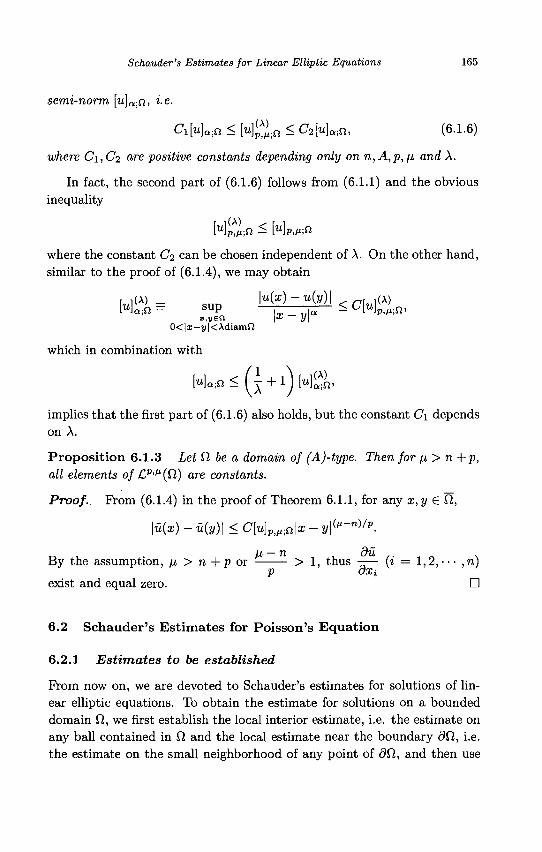
Schauder's Estimates for Linear Elliptic Equations 165
semi-norm [u]a-n, i.e.
C i M a i n < H ^ i n < C , 2 [ « ] a i n , (6.1.6)
where C\,C2 are positive constants depending only on n,A,p,/i and A.
In fact, the second part of (6.1.6) follows from (6.1.1) and the obvious inequality
MiJU < ("]p,wn
where the constant Ci can be chosen independent of A. On the other hand, similar to the proof of (6.1.4), we may obtain
\u]W = SUD Hx)-U(y)\ (A)
i,»en I J> i/| 0<|x—y|<Adiam£2
which in combination with
[u]«;n<Q + l)[u£ (A)
implies that the first part of (6.1.6) also holds, but the constant C\ depends on A.
Proposition 6.1.3 Let O be a domain of (A)-type. Then for fi> n + p, all elements of £P'M(Q) are constants.
Proof. Prom (6.1.4) in the proof of Theorem 6.1.1, for any x, y £ Cl,
\u(x)-u(y)\<C[u}p^u\x-y\^-n^.
_ , , . ^ — n , , d u , . , n . By the assumption, fx > n + p or > 1, thus —— n = 1,2, • • • , n)
p dXi exist and equal zero. •
6.2 Schauder's Estimates for Poisson's Equation
6.2.1 Estimates to be established
From now on, we are devoted to Schauder's estimates for solutions of linear elliptic equations. To obtain the estimate for solutions on a bounded domain Q, we first establish the local interior estimate, i.e. the estimate on any ball contained in fl and the local estimate near the boundary dCl, i.e. the estimate on the small neighborhood of any point of dCl, and then use
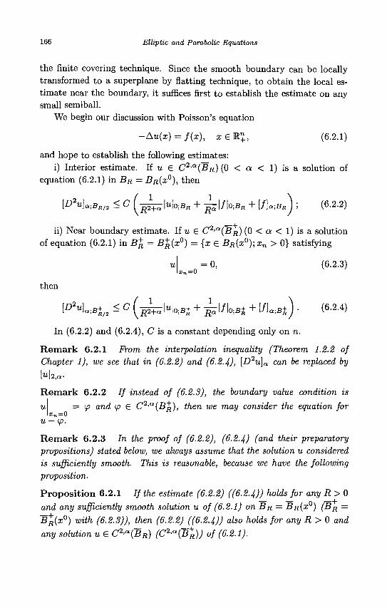
166 Elliptic and Parabolic Equations
the finite covering technique. Since the smooth boundary can be locally transformed to a superplane by flatting technique, to obtain the local estimate near the boundary, it suffices first to establish the estimate on any small semiball.
We begin our discussion with Poisson's equation
-Au(x) = f(x), x £ Rl, (6.2.1)
and hope to establish the following estimates: i) Interior estimate. If u £ C2'a(BR)(0 < a < 1) is a solution of
equation (6.2.1) in BR = BR(X°), then
[D2u]a;BR/2 < C ( - ^ \U\0,BR + - ^ | / | 0 ; B R + [/]Q;Bfl) ; (6.2.2)
ii) Near boundary estimate. If u £ C2'a{BR) (0 < a < 1) is a solution of equation (6.2.1) in J5^ = B^(x°) = {x £ BR{XQ);XU > 0} satisfying
0, (6.2.3) x„=0
then
P a < B j „ * C ( ^ > I O ; B + + ^ I / I O ; B + + I / U j ) • (6-2-4)
In (6.2.2) and (6.2.4), C is a constant depending only on n.
R e m a r k 6.2.1 From the interpolation inequality (Theorem 1.2.2 of Chapter 1), we see that in (6.2.2) and (6.2.4), [D2u]a can be replaced by
M2,a-
R e m a r k 6.2.2 / / instead of (6.2.3), the boundary value condition is
u = <p and tp € C2'a(B~ft), then we may consider the equation for xn=0
u — ip.
R e m a r k 6.2.3 In the proof of (6.2.2), (6.2.4) (and their preparatory propositions) stated below, we always assume that the solution u considered is sufficiently smooth. This is reasonable, because we have the following proposition.
Proposi t ion 6.2.1 / / the estimate (6.2.2) ((6.2.4)) holds for any R>0
and any sufficiently smooth solution u of (6.2.1) on BR = BR(X°) (BR =
~B+R{xQ) with (6.2.3)), then (6.2.2) ((6.2.4)) also holds for any R>0 and
any solution u £ C2>a{BR) (C2^(BR)) of (6.2.1).
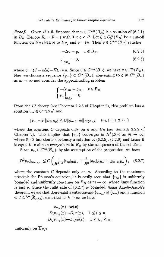
Schauder's Estimates for Linear Elliptic Equations 167
Proof. Given R > 0. Suppose that u £ C2'a(BR) is a solution of (6.2.1) in BR. Denote Re = R-e with 0 < e < R. Let £ e Cfi°(BR) be a cut-off function on BR relative to BRC and v = £u. Then v £ C2'a(BR) satisfies
-Av = g, x£ BR, (6.2.5)
= 0, (6.2.6) dBR
where g = £f - uA£ - V£ • Vtt. Since u € C2'a(BR), we have g € Ca(BR). Now we choose a sequence {ffm} C C°°(BR), converging to g in Ca(BR) as m —• co and consider the approximating problem
XGBR,
Prom the L2 theory (see Theorem 2.2.5 of Chapter 2), this problem has a solution vm £ C°°(BR) and
\\Vm -Vl\\H*(BR) < C\\9m-gi\\L*(BR), ( " I , / = 1, 2, • • • )
where the constant C depends only on n and B« (see Remark 2.2.2 of Chapter 2). This implies that {vm} converges in H2(BR) as m —> oo, whose limit function is obviously a solution of (6.2.5), (6.2.6) and hence it is equal to v almost everywhere in BR by the uniqueness of the solution.
Since vm € C°°(BR), by the assumption of the proposition, we have
[D2Vm}a]BR/2 < C ( ^2+S>m|0;B* + -j^\9mW,BR + [9m]a;BR J , (6.2.7)
where the constant C depends only on n. According to the maximum principle for Poisson's equation, it is easily seen that {vm} is uniformly bounded and uniformly converges on BR as m —• oo, whose limit function is just v. Since the right side of (6.2.7) is bounded, using Arzela-Ascoli's theorem, we see that there exist a subsequence {vmk} of {vm} and a function w € C2'a(BR/2), such that as k —> oo we have
Vmk{x)->w(x),
DiVmk(x)->Diw(x), 1 < i < n,
Dijvmk(x)-^Dijw(x), l<i,j<n,
uniformly on BR/2-
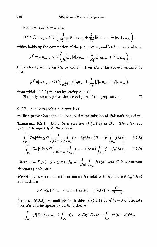
168 Elliptic and Parabolic Equations
Now we take m = rrik in
[D Vm]a;BRc/2 < C ( R2+a\vm\o;BRe + -j^\9m\o;BRs + [9m]a;BRc J ,
which holds by the assumption of the proposition, and let k —> oo to obtain
\D2wUBRc/2 < C l^^\v\0.BRc + -j^\g\0;BRc + [g]a;BReJ ,
Since clearly w = v on BRe/2 and £ = 1 on BRC, the above inequality is just
\D2uUBRc/2 < C(-jJ2+^W\0;BRc + - ^ I / I O J B K , + [f]a;BRt),
from which (6.2.2) follows by letting e —> 0 + . Similarly we can prove the second part of the proposition. •
6.2.2 Caccioppoli's inequalities
we first prove Caccioppoli's inequalities for solution of Poisson's equation.
Theorem 6.2.1 Let u be a solution of (6.2.1) in BR. Then for any 0 < p < R and A € i , there hold
[ \Du\2dx<c\.0 -1 . - / (u-X)2dx+(R-p)2 [ f2dx], (6.2.8) JB„ <-{R-P) JBR JBR
J
L \Dw\2dx<C (R
^ f (w-X)2dx+[ (f-fR)2dx\, (6.2.9) - PYJBR JBR J
where w = Diu{l < i < n), fR = / f(x)dx and C is a constant \BR\ JBR
depending only on n.
Proof. Let 77 be a cut-off function on BR relative to Bp, i.e. 77 6 CQ°(BR) and satisfies
C 0 < T)(x) < 1, r)(x) = 1 in Bp, \Dr](x)\ <
R- p
To prove (6.2.8), we multiply both sides of (6.2.1) by rj2(u — A), integrate over BR and integrate by parts to derive
/ T]2\Du\2dx =-2 j rj{u - \)Drj • Dudx + r]2(u-\)fdx. JBR JBR JBR
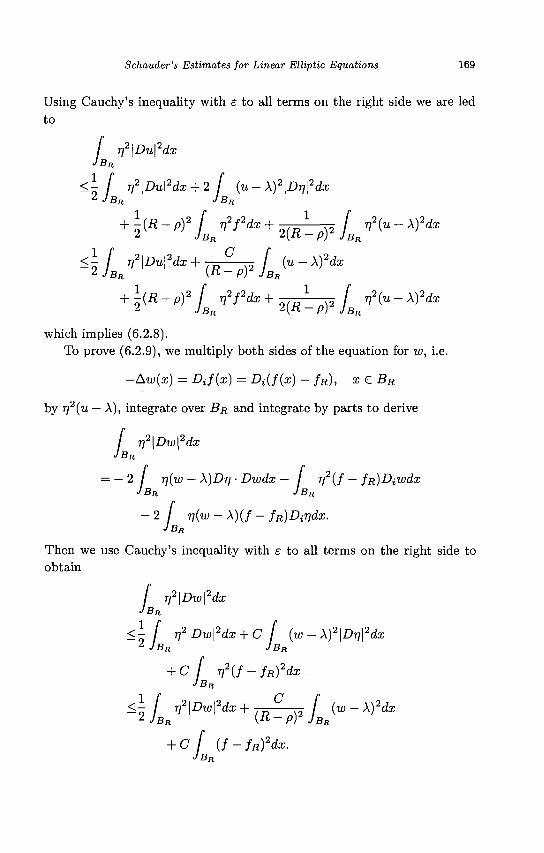
Schauder's Estimates for Linear Elliptic Equations 169
Using Cauchy's inequality with e to all terms on the right side we are led to
/ r]2\Du\2dx JBR
<\ I r)2\Du\2dx + 2 [ (u-X)2\Dr,\2dx 2 J BR J BR
which implies (6.2.8).
To prove (6.2.9), we multiply both sides of the equation for w, i.e.
-At»( i ) = Dif(x) = Di(f(x) - f R ) , xeBR
by T]2(U — A), integrate over BR and integrate by parts to derive
/ ri2\Dw\2dx JBR
= - 2 / n(w- \)Dr) • Dwdx - f n2(f - fR)Diwdx JBR JBR
- 2 / v(w-\)(f- fR)Dir1dx. JBR
Then we use Cauchy's inequality with e to all terms on the right side to obtain
/ r)2\Dw\2dx JBR
<\ I r)2\Dw\2dx + C f (w - X)2\Dr]\2dx 2 JBR JBR
+ C f V2(f~fR)2dx JBR
/ (f-M* JBR
C (/ - fRYdx. IBR
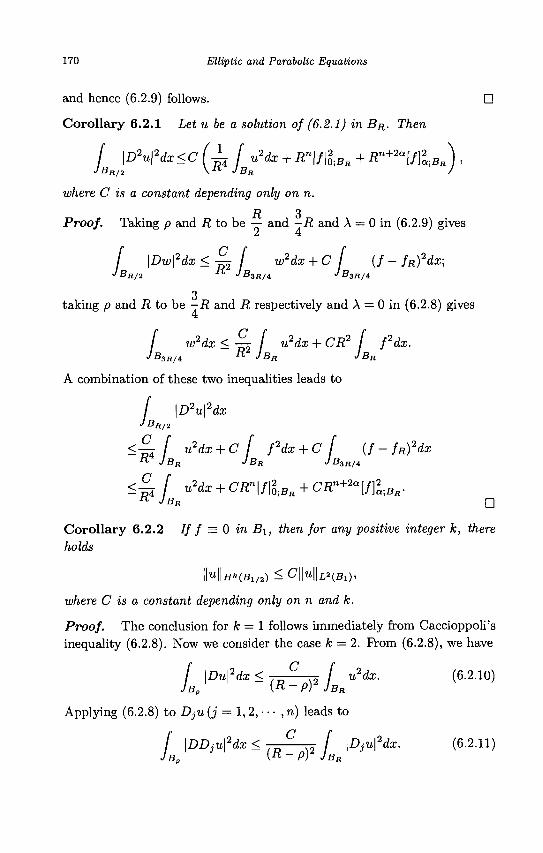
170 Elliptic and Parabolic Equations
and hence (6.2.9) follows. •
Corollary 6.2.1 Let u be a solution of (6.2.1) in BR. Then
JB \D2u\2dx<C (± j B u2dx + Rn\f\20,BR + Rn+2a[f}l,B^ ,
where C is a constant depending only on n.
Proof. Taking p and R to be — and -R and A = 0 in (6.2.9) gives
f \Dw\2dx < jL J w2dx + C f (f- fR)2dx; JBRI2 JB30/4 •'B3R/4 ?R/2 J &3R/4 JD3R/4
3 taking p and R to be -R and R respectively and A = 0 in (6.2.8) gives
/ w2dx < - ^ / u2dx + CR2 f fdx. JB3R/4 R JBR JBn
A combination of these two inequalities leads to
f \D2u\2dx
<£z f u2dx + C f f2dx + C f {f-fR)2dx R JBR JBR JB3R/i
< | _ f u2dx + CRn\f\l,BR + CR^2a[f}2a,BR.
K JBR •
Corollary 6.2.2 If f = 0 in B\, then for any positive integer k, there holds
IMItf*(B1/2) < C||W||L J(BI)»
where C is a constant depending only on n and k.
Proof. The conclusion for fc = 1 follows immediately from Caccioppoli's inequality (6.2.8). Now we consider the case fc = 2. Prom (6.2.8), we have
[ \Du\2dx < — ^ / u2dx. (6.2.10) JBP {R-PY JBR
Applying (6.2.8) to DjU (j = 1,2, • • • , n) leads to
/ \DDjU\2dx < .J3 ,2 f \DjU\2dx. (6.2.11) JBD {R ~ P) JBR
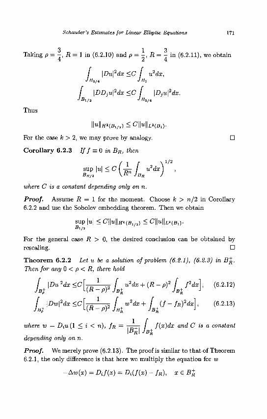
Schauder 's Estimates for Linear Elliptic Equations 171
3 1 3 Taking p = -, R = 1 in (6.2.10) and p = - , R = - in (6.2.11), we obtain
J \Du\2dx <C f u2dx, J B3/4 J B\
j \DDju\2dx <C J \Dju\2dx. JBx/2 JB3/I
Thus
IMIff*(B1/a) < C||u| |L2 (B l ) .
For the case k > 2, we may prove by analogy. •
Corollary 6.2.3 lff = 0in BR, then
sup \u\ < C ( — / u2dx I BR/2 \ K JBR J
where C is a constant depending only on n.
Proof. Assume R = 1 for the moment. Choose k > n/2 in Corollary 6.2.2 and use the Sobolev embedding theorem. Then we obtain
SUp \u\ < C | | u | | f f f c ( B l / 2 ) < C | | u | | L 2 ( B l ) . B1/2
For the general case R > 0, the desired conclusion can be obtained by rescaling. •
Theo rem 6.2.2 Let u be a solution of problem (6.2.1), (6.2.3) in B^. Then for any 0 < p < R, there hold
j \Du\2dx<c\,„ l so f u2dx + (R-p)2 [ f2dx\, (6.2.12)
JB+ 1(R-P) JB+ JB+ J
/ \Dw\2dx<c\.u l j w2dx+ [ (f-fR)2dx\, (6.2.13)
JB+ l(R-prJB+ JB+ J
where w — Diu(l < i < n), / » = -—xr / f(x)dx and C is a constant
depending only on n.
Proof. We merely prove (6.2.13). The proof is similar to that of Theorem 6.2.1, the only difference is that here we multiply the equation for w
- A » ( i ) = Dif{x) = Di(f(x) - / „ ) , x&B+
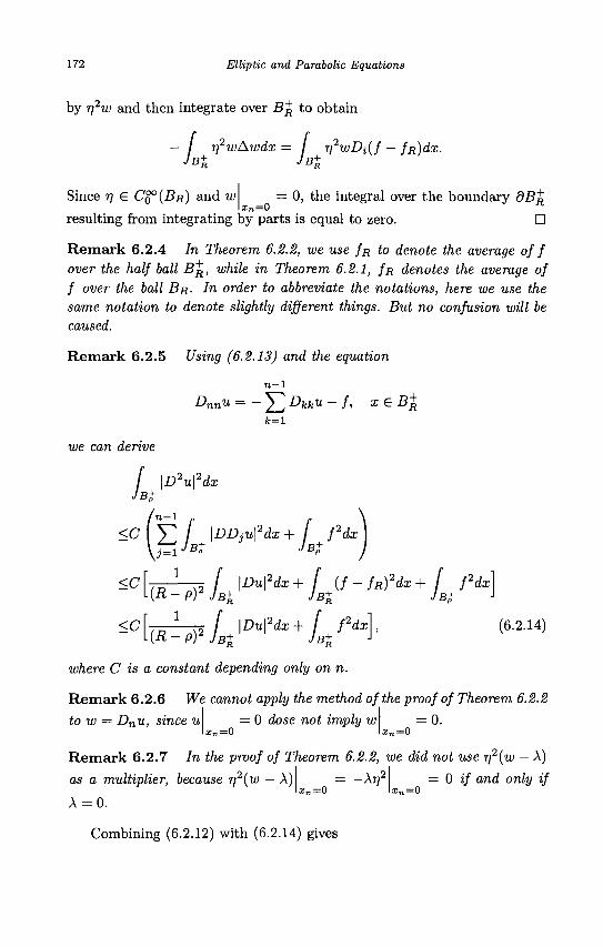
172 Elliptic and Parabolic Equations
by r)2w and then integrate over JB^ to obtain
- / T]2wAwdx = / n2wDi(f - fR)dx. JB+ JB+
Since n € C^(BR) and w xn=0
0, the integral over the boundary dB^
resulting from integrating by parts is equal to zero. • Remark 6.2.4 In Theorem 6.2.2, we use fa to denote the average of f over the half ball B^, while in Theorem 6.2.1, $R denotes the average of f over the ball BR. In order to abbreviate the notations, here we use the same notation to denote slightly different things. But no confusion will be caused.
Remark 6.2.5 Using (6.2.13) and the equation
n - l
L'nn'U' = ~ 2 DkkU ~ f> xeBR fc=l
we can derive
L \D2u\2dx
<C\Y f \DDjU\2dx + [ fdx I \J=W jBt )
<C
<c
(R
(R
dx+ / (f-fR)2dx
• l ^ j / \Du\2dx+ [ fdx - P)2 JBt JBt
f fdx JBt
(6.2.14)
where C is a constant depending only on n.
Remark 6.2.6 We cannot apply the method of the proof of Theorem 6.2.2
to w = Dnu, since u x n =0
= 0 dose not imply w x„=0
0.
Remark 6.2.7 In the proof of Theorem 6.2.2, we did not use n2{w — A)
as a multiplier, because r)2(w — A)
A = 0. x n =0
= -Xrf xn=0
= 0 if and only if
Combining (6.2.12) with (6.2.14) gives
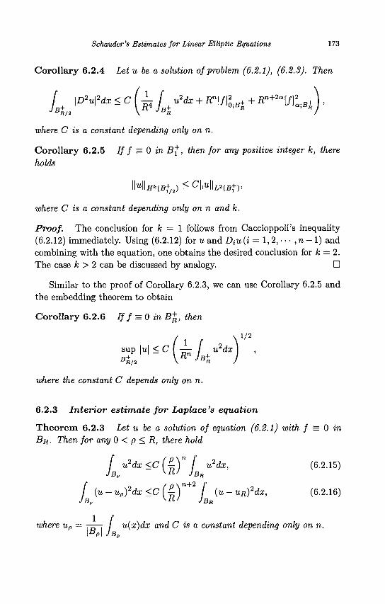
Schauder's Estimates for Linear Elliptic Equations 173
Corollary 6.2.4 Let u be a solution of problem (6.2.1), (6.2.3). Then
j \D2u\2dx < C (^ J u2dx + R«KB+R + R^[fl,B+) ,
where C is a constant depending only on n.
Corollary 6.2.5 If f = 0 in B*, then for any positive integer k, there holds
\\U\\H"(B+/2) ^ C 'IIUIIL2(B+)>
where C is a constant depending only on n and k.
Proof. The conclusion for fc = 1 follows from Caccioppoli's inequality (6.2.12) immediately. Using (6.2.12) for u and DiU (i = 1,2, • • • , n — 1) and combining with the equation, one obtains the desired conclusion for fc = 2. The case k > 2 can be discussed by analogy. •
Similar to the proof of Corollary 6.2.3, we can use Corollary 6.2.5 and the embedding theorem to obtain
Corollary 6.2.6 If f = 0 in B^, then
1/2 (i r V
sup \u\ < C I —- / u2dx ,
where the constant C depends only on n.
6.2.3 Interior estimate for Laplace's equation
Theorem 6.2.3 Let u be a solution of equation (6.2.1) with f = 0 in BR. Then for any 0 < p < R, there hold
I u2dx<c(^Y I u2dx, (6.2.15) JBP
v # y JBR
I (u-up)2dx<c(£)n I (u-uR)2dx, (6.2.16)
JBP ^RJ JBR
where up = . . / u(x)dx and C is a constant depending only on n. \BP\ JBD
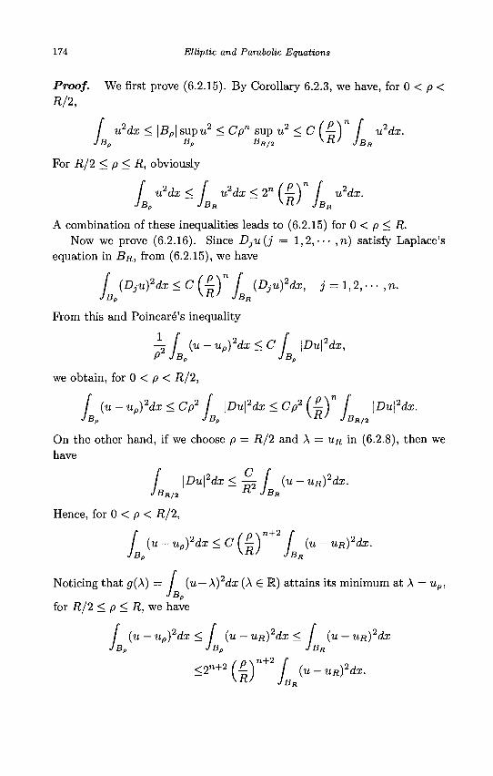
174 Elliptic and Parabolic Equations
Proof. We first prove (6.2.15). By Corollary 6.2.3, we have, for 0 < p < R/2,
/ u2dx < \BP\ supu2 < Cpn sup u2 < C (^Y [ u2dx. JB„ B„ BR/2 Vi t / JBR
For R/2 < p<R, obviously
/ u2dx < f u2dx < 2" (~Y / u2dx. JB„ JBR
yRJ JBR
A combination of these inequalities leads to (6.2.15) for 0 < p < R. Now we prove (6.2.16). Since Dju(j = 1,2, ••• ,n) satisfy Laplace's
equation in BR, from (6.2.15), we have
j (DjU)2dx < C ( ^ ) " J (DjU)2dx, j = 1,2, • • • ,n.
From this and Poincare's inequality
~2 / (u — up)2dx <C \Du\2dx,
P JBP JB„
we obtain, for 0 < p < R/2,
[ (u - up)2dx < Cp2 [ \Du\2dx < Cp2 ( • § ) " / \Du\2dx.
JB„ JB„ XR) JBRn
On the other hand, if we choose p = R/2 and A = UR in (6.2.8), then we have
/ \Du\2dx <% f (u - uR)2dx. JBR/2
K JBa
Hence, for 0 < p < R/2,
f {u-up)2dx<c(^)n+2 f (u-uR)2dx.
JBp JBR
Noticing that g(X) = / (u — X)2dx (A £ R) attains its minimum at A = up, JBP
for R/2 < p < R, we have
/ (u — up)2dx < (u — UR)2dx < j {u — UR)2dx
JBp JBP JBR
< 2 " + 2 ( | ) n + 2 y (u-uR)2dx.
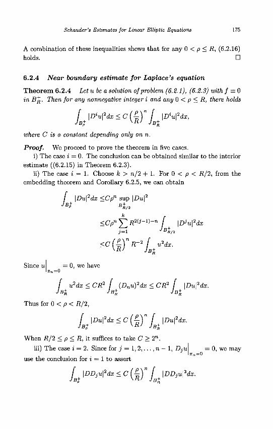
Schauder's Estimates for Linear Elliptic Equations 175
A combination of these inequalities shows that for any 0 < p < R, (6.2.16) holds. •
6.2.4 Near boundary estimate for Laplace's equation
Theorem 6.2.4 Let u be a solution of problem (6.2.1), (6.2.3) with / = 0 in Bft. Then for any nonnegative integer i and any 0 < p < R, there holds
f ID^dx^cl^-Y f iD^dx, JB+ \R' JB+
where C is a constant depending only on n.
Proof. We proceed to prove the theorem in five cases. i) The case i = 0. The conclusion can be obtained similar to the interior
estimate ((6.2.15) in Theorem 6.2.3). ii) The case i = 1. Choose k > n/2 + 1. For 0 < p < R/2, from the
embedding theorem and Corollary 6.2.5, we can obtain
/ . Bi K/2
\Du\2dx <Cpn sup \Du\2
B£/2 k .
<Cpn^2R2{j-1)-n \Dju\2dx
'<
Since u — 0, we have xn=0
f u2dx < CR2 f (Dnu)2dx < CR2 [ \Du\2dx. JB+
R JB+ JB+
Thus for 0 < p < R/2,
I \Du\2dx<c(^Y f \Du\2dx. JB+ ^ttJ
JB+ JR
When R/2 < p < R, it suffices to take C > 2n.
hi) The case i = 2. Since for j = 1,2,. . . , n — 1, DjU
use the conclusion for i = 1 to assert
= 0, we may xn=0
f \DDjU\2dx<c(£)n f \DDjU\2dx.
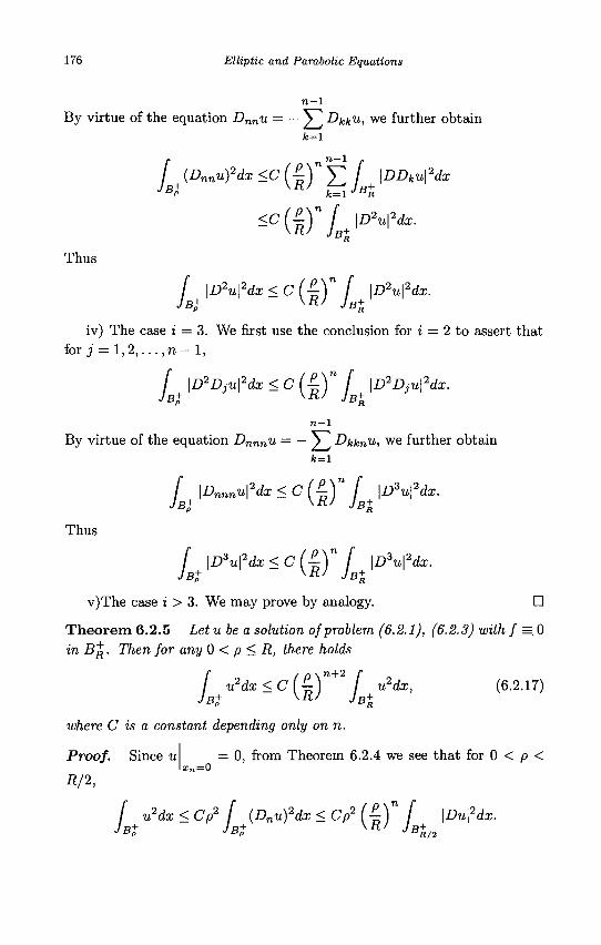
176 Elliptic and Parabolic Equations
n - 1
By virtue of the equation Dnnu = — V^ DkkU, we further obtain fe=i
n-\
Thus
/ {Dnnufdx <C (-§) V / \DDku\2dx JBt KRJ £^IJB+R
/ |D2u|2dx < C (4)" / |£>2u|2dx.
iv) The case i = 3. We first use the conclusion for i = 2 to assert that for j = 1 , 2 , . . . , n - l ,
/ |I>2I>7-u|2da; < C f ^ " / |£>2£>,u|2cfc.
n - l
By virtue of the equation Dnnnu = — YJ DkknU, we further obtain fc=i
/ \Dnnnu\2dx<c(£)n [ \D3u\2dx. JB+ ^RJ JB+
Thus
f + \D3u\2dx < C ( | ) n f + \D3u\2dx.
v)The case i > 3. We may prove by analogy. •
Theorem 6.2.5 Let u be a solution of problem (6.2.1), (6.2.3) with / = 0 in B'R . Then for any 0 < p < R, there holds
f u2dx<c(^-)n+2 f u2dx, (6.2.17) JB+ XRJ JB+
where C is a constant depending only on n.
Proof. Since u
R/2, x = 0
0, from Theorem 6.2.4 we see that for 0 < p <
f u2dx < Cp2 f (Dnu)2dx < Cp2 ( •§ ) " / \Du\2dx. JB+ JB+ V ^ JB+/2
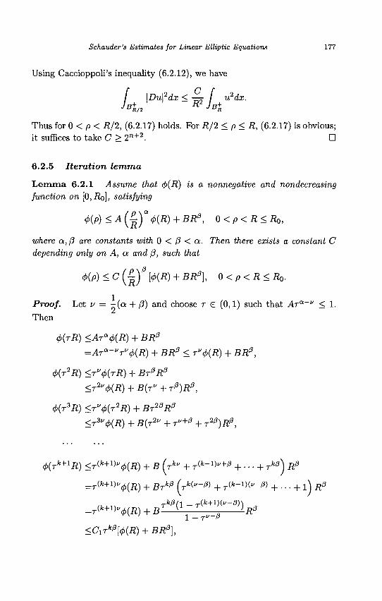
Schauder's Estimates for Linear Elliptic Equations 177
Using Caccioppoli's inequality (6.2.12), we have
/ \Du\2dx <-^[ u2dx. JB+,„ R JB+ JR/2
Thus for 0 < p < R/2, (6.2.17) holds. For R/2 < p < R, (6.2.17) is obvious; it suffices to take C > 2"+2. •
6.2.5 Iteration lemma
Lemma 6.2.1 Assume that <f>(R) is a nonnegative and nondecreasing function on [0,Ro], satisfying
4>(p)<A^y4>{R) + BR0, 0<p<R<R0,
where a, (3 are constants with 0 < 8 < a. Then there exists a constant C depending only on A, a and 0, such that
<p(p)<C^y[cf)(R) + BR13}, 0<p<R<Ro.
Proof. Let v = -(a + 0) and choose r € (0,1) such that AT01'" < 1.
Then
(J){TR) <Ara(f)(R) + BR0
=ATa-/T»4>{R) + BR0 < T"4>{R) + BR0,
4>{T2R) <TU<J>(TR) + BT0R0
<T2V4>(R) + B{TV + T0)R0,
4>(T3R) <TV(J>{T2R) + BT20R0
<T3V<P(R) + B(T2V + TU+0 + T20)R0,
<j>{rk+1R) <T^k+1^4>(R) + B (rkv + T^-l>+0 + ••• + rk0) R0
=r(fc+1>"0(fl) + Brk0 (,><"-« + T^-^v~^ + • • • + l ) R0
=r^>4>{R) + BT ( 1 ~ r ' V
<CiTk0[</>(R) + BR0},
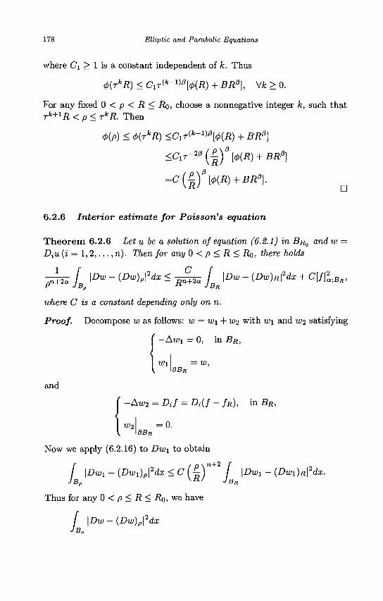
178 Elliptic and Parabolic Equations
where C\ > 1 is a constant independent of k. Thus
cj){TkR) < CITV-WMR) + BRf3}, Vfc > 0.
For any fixed 0 < p < R < Ro, choose a nonnegative integer k, such that rk+1R <p< rkR. Then
4>(p) < <t>(TkR) <ClT^k-1^[<j>{R)+BRp]
<C,r-^{^[4>{R)+BR^
=c(£fMR)+BB?].
6.2.6 Interior estimate for Poisson's equation
Theorem 6.2.6 Let u be a solution of equation (6.2.1) in £?R0 and w = DiU (i = 1,2,. . . , n). Then for any 0 < p < R< RQ, there holds
- L ; / \Dw- (Dw)p\2dx < - g ^ / \Dw - (Dw)R\2dx + C[f]%BR,
where C is a constant depending only on n.
Proof. Decompose w as follows: w = wi + u>2 with wi and w^, satisfying
-Atoi = 0, in BR,
WI dBE
= W,
and
-Aw2 = Dif = Di(f - f R ) , in BR,
W2 dBR
0.
Now we apply (6.2.16) to Dw\ to obtain
/ \DWl-{DWl)p\2dx<c(^)n^ f \DWl-{DWl)R\2dx.
JBP XK/ JBR
Thus for any 0 < p < R < Ro, we have
/ \Dw - (Dw)p\2dx
JBD
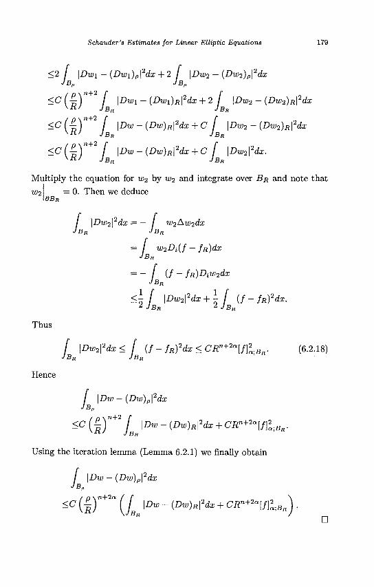
Schauder's Estimates for Linear Elliptic Equations 179
<2 / \Dwi - (Dwi)p\2dx + 2 / \Dw2 - (Dw2)p\
2dx JBP JBP
<C(^Y+2 f \DWl-(DWl)R\2dx + 2 f \Dw2-(Dw2)R\2dx yii/
JBR JBR
<C ( | ) " + 2 / \Dw - (Dw)R\2dx + C f \Dw2 - (Dw2)R\2dx JBR JBR
<C(^-Y+2 f \Dw-(Dw)R\2dx + C f \Dw2\2dx.
KRJ JBR J BR
Multiply the equation for w2 by w2 and integrate over BR and note that
w2 = 0 . Then we deduce dBR
I \Dw2\2dx — — I w2Aw2dx
JBR JBR
= I w2Di(f - fR)dx JBR
= ~ {f - fR)DiW2dx J BR
<\f \Dw2\2dx + \f (f-fR)2dx.
J BR " JBR
Thus
f \Dw2\2dx < / " ( / - fR)2dx < CRn+2a[f}2
a.BR. (6.2.18) JBR JBR > BR
Hence
/ \Dw - (Dw)p\2dx
JBP
~C (RT+2 jBR
lDW - ^W^\2dX + CRn+2alft,BR-
Using the iteration lemma (Lemma 6.2.1) we finally obtain
/ \Dw-{Dw)p\2dx
JBP
~C ( | ) " + 2 a (JBR \DW - (Dw)x\2d* + C*n+2alf}l;BR) • a
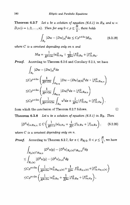
180 Elliptic and Parabolic Equations
Theorem 6.2.7 Let u be a solution of equation (6.2.1) in BR and w =
DiU (i = 1,2 , . . . ,n) . Then for any 0 < p < —, there holds
f \Dw-(Dw)p\2dx<Cpn+2aMR, (6.2.19)
JBP
where C is a constant depending only on n and
Proof. According to Theorem 6.2.6 and Corollary 6.2.1, we have
/ \Dw - (Dw)p\2dx
JBP
^Pn+2a ( ^ k JBR/2 \DW ~ (Dw)R/2\2dx + lf}i]BR/)j
^ + 2 " ( ^ W / B R / 2 I ^ I ^ + [ / I U / 2 )
^Pn+2a { j ^ JBR u2dx + ^ I / I U + \f]l,BR) ,
from which the conclusion of Theorem 6.2.7 follows. •
Theorem 6.2.8 Let u be a solution of equation (6.2.1) in BR. Then
[D2u]a;BR/2 < C (^^\U\0;BR + ^\f\o-,BR + [ / U B K ) , (6.2.20)
where C is a constant depending only on n.
Proof. According to Theorem 6.2.7, for x G BR/2, 0 < p < —, we have
/ \D2u(y)-(D2u)Bp{x)nBR/2\2dy
JBp(x)f\BR/2
< f \D2u(y) - (D2u)XtP\2dy
JBp{x)
<Cpn+ a f Ri+2a \U\o;BR/2(x) + - ^ l/lo;BH/2(x) + U\a;BR/2(x)
^ P ^ ( j ^ \ < B R + ^\f\l,BR + [ft,BR) ,
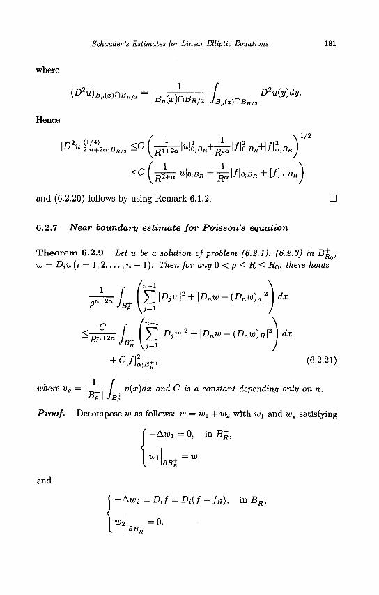
Schauder's Estimates for Linear Elliptic Equations 181
where
Hence
(D2u)B{x)r)B = } - / D2u(y)dy K/i \Bp{x)r\BR/2\ JBp(x)nBR/2
1/2
[D U]2,n+2a;BR/2 ^ ( p 4 + 2 a \U\o;BR+^2^\f\o;BR+[f]a;BR )
and (6.2.20) follows by using Remark 6.1.2. D
6.2.7 Near boundary estimate for Poisson's equation
Theorem 6.2.9 Let u be a solution of problem (6.2.1), (6.2.3) in B^, w = DiU (i = 1,2,. . . , n — 1). Then for any 0 < p < R < Ro, there holds
• ^ jB+ ( E l^ 'H2 + \Dnw - (Dnw)p\2 J dx
^J^ fg+ f E \Diwf + \D"W ~ (A^)fil2 dx
+ c[f)lBt, (6.2.21)
where vp = , / v(x)dx and C is a constant depending only on n. \BP I JB+
Proof. Decompose w as follows: w = W1+W2 with w\ and u>2 satisfying
' -Awi = 0, in B^,
w 9Bt
and
' -Aw2 = Dif = Di(f - f R ) , in B+,
V)2 dBl
0.
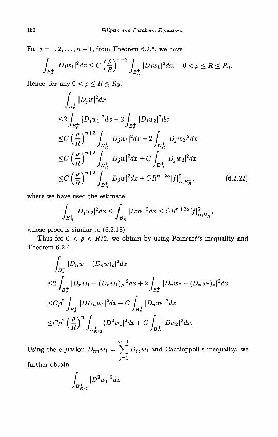
182 Elliptic and Parabolic Equations
For j' — 1,2,. . . , n — 1, from Theorem 6.2.5, we have
/ IDjWifdxKCf^Y / IDjWxfdx, 0<P<R<RQ. JB+ v-fty JB+
Hence, for any 0 < p < R < Ro,
/ \Djw\2dx JB+
<2 \DjWi\2dx + 2 \DjW2\2dx
J Bp J Bp
< C ( 4 ) " + 2 / \DjWl\2dx + 2 f \DjW2\
2dx v-ft' JB+ JB+
<C(^Y+ f \DjW\2dx + C f \DjW2\2dx
<C ( |)"+2 j + \DjW\2dx + CRn+2a[f}2a;B+R, (6.2.22)
where we have used the estimate
/ \DjW2\2dx< f \Dw2\
2dx<CRn+2a[f]2B+,
JB+ JB+
whose proof is similar to (6.2.18). Thus for 0 < p < R/2, we obtain by using Poincare's inequality and
Theorem 6.2.4,
/ \Dnw - (Dnw)p\2dx
JB+
<2 / \Dnwi - (Dnwi)p\2dx + 2 \Dnw2 - {Dnw2)p\
2dx JB+ JB+
<Cp2 / \DDnwx\2dx + C / \Dnw2\
2dx JB+ JB+
<Cp2(^Y f \D2Wl\
2dx + C f \Dw2\2dx.
^R' JB+„ JB+ JR/2
n-\ Using the equation DnnW\ = )> DjjW\ and Caccioppoli's inequality, we
further obtain
/ \D2wi?dx JB+,„
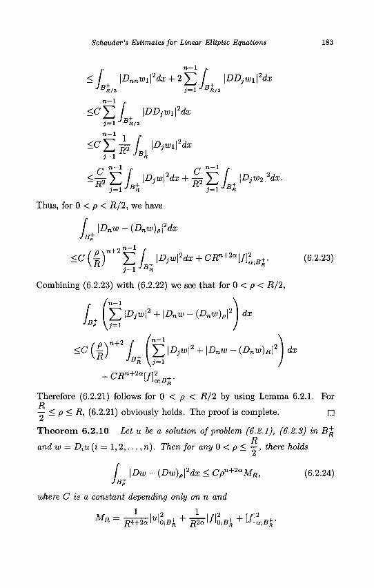
Schauder's Estimates for Linear Elliptic Equations 183
< / \Dnnwi\2dx + 2 V / \DDjWi\2dx JB+/2 , = 1 JB+„
n—l .
DR/2 j = l DR/1
n-1
\DDjWi?dx /R+
7 1 - 1
417B. |^ |2^+^l14 i^2|2da:-Thus, for 0 < p < R/2, we have
\Dnw - (Dnw)p\2dx
, 7 1 - 1
/ .
^ ( 4 ) " + 2 E / l ^^ | 2 ^ + Ci?"+2a[/]^+. (6.2.23) XK/ J=IJBR
Combining (6.2.23) with (6.2.22) we see that for 0 < p < R/2,
I V] \DjW\2 + \Dnw - (Dnw)p\2 dx
JB* \i=i )
,2 p I n—l \
-C(R) I + I S l^wl2 + l £ > n U '~ (£ >"u ,)«l2 dx
+ C i r , + 2 a [ / ] 2 ; B i -
Therefore (6.2.21) follows for 0 < p < R/2 by using Lemma 6.2.1. For
— < p < R, (6.2.21) obviously holds. The proof is complete. •
Theorem 6.2.10 Let u be a solution of problem (6.2.1), (6.2.3) in B^
and w = DiU (i = 1,2,.. . , n). Then for any 0 < p < —, there holds
L \Dw - (Dw)p\*dx < Cpn+^aMR, (6.2.24) B+
where C is a constant depending only on n and
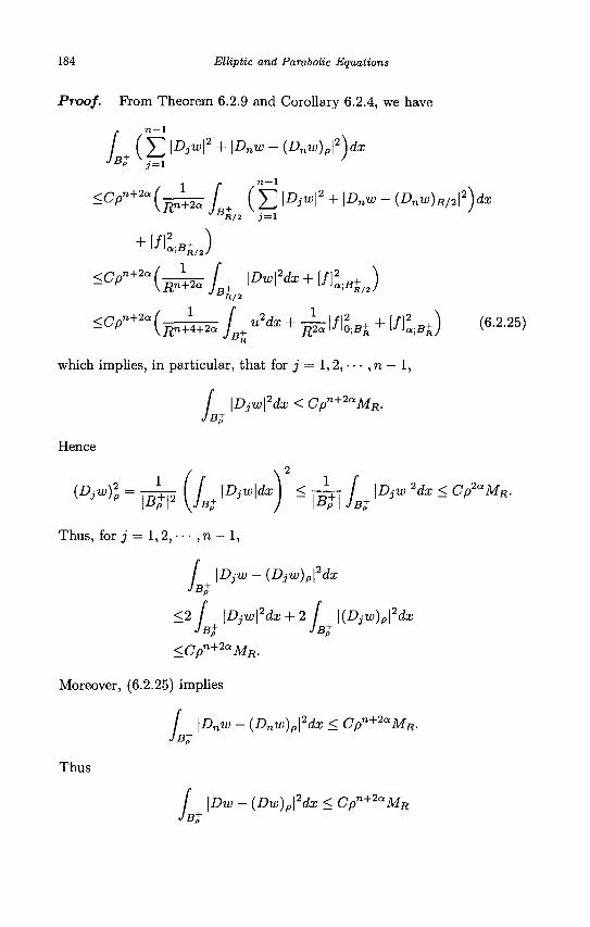
184 Elliptic and Parabolic Equations
Proof. From Theorem 6.2.9 and Corollary 6.2.4, we have
~ 71— 1
/ ( ^ \DjW\2 + \Dnw - {Dnw)p\2\dx
JB+ j=1
JBR/2 j = l
^n+2a(^lBJD^d^KBR/2) ^f>n+2a ( ^ jB+ «
2*° + j^Mrt + K*)
which implies, in particular, that for j = 1,2, • • • , n — 1,
/ \Djw\2dx < CPn+2aMR.
JBt
Hence
(DjW)2p = - J j - ( / IZ -Hdz J < 7 +7 / + l-D^I2^ <
Thus, for j = 1,2, • • • , n — 1,
/ \DjW — (Djw)p\2dx
JB+
<2 / \D1w\2dx + 2 / |(£>,u))pl2da;
i s+ JB+
<Cpn+2aMR.
Moreover, (6.2.25) implies
[ \Dnw - (Dnw)p\2dx < Cpn+2aMR.
Thus
/ \Dw - {Dw)p\2dx < Cpn+2aMR
JB+
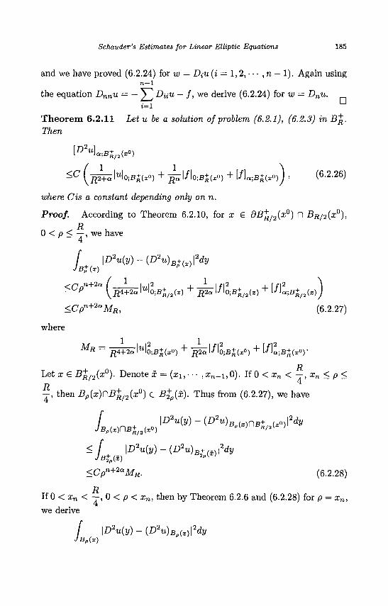
Schauder's Estimates for Linear Elliptic Equations 185
and we have proved (6.2.24) for w — DiU (i — 1,2, • • • , n — 1). Again using n - l
the equation Dnnu •= — V^ Duu — / , we derive (6.2.24) for w = Dnu. i=l
Theorem 6.2.11 Let u be a solution of problem (6.2.1), (6.2.3) in B^. Then
[£ 2 < ; B + / 2 (x°)
^C ( fi2+^ Ho;B+(xO) + ^ l/lo;B+(xO) + [/]a;B+(x<>) J , (6.2.26)
where Cis a constant depending only on n.
Proof. According to Theorem 6.2.10, for x € dB^/2(x°) n BR/2(x°),
0 < p < - j i we have
/ \DMy)-(D2u)BUx)fdy
<CPn+2a \j^^-\u\liB+^x) + - ^ | / l o ; B + / 2 ( x ) + [ /]a i B+ / 2(x)J
<Cpn+2aMR, (6.2.27)
where
1 . ., . 1 .-,2 ^ #4+2a N();B+(x°) + #2a l'lo;B+(i°) + V ia;B+(x°
Let x e B^^2(x°). Denote x = (xi,- •• , x n _i ,0 ) . If 0 < xn < —, xn < p <
—, then Bp(x)nB+/2(x°) C B%p{x). Thus from (6.2.27), we have
</" | D V I / ) - ( ^ 2 « ) B + ( 2dt/
<Cpn+2aMR. (6.2.28)
If 0 < xn < —, 0 < p < xn, then by Theorem 6.2.6 and (6.2.28) for p = xn,
we derive
/ \D2u(y)-(D2u)Bf>{x)\2dy
JB„(x)
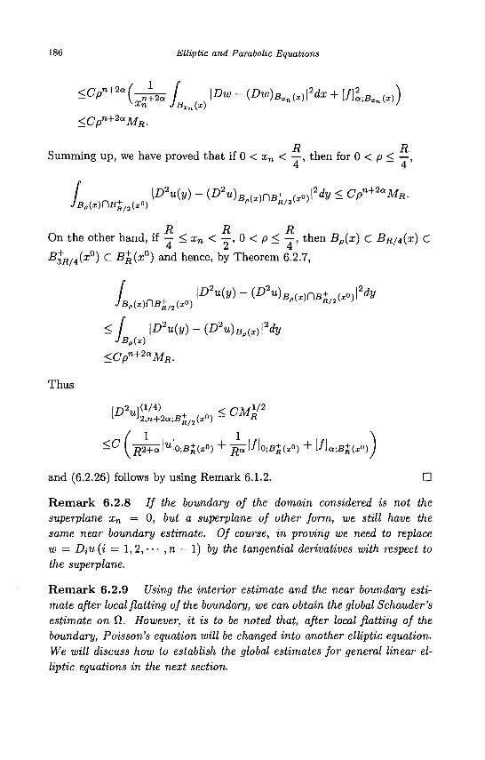
186 Elliptic and Parabolic Equations
<CPn+2a(-^ f r\Dw-(Dw)Bxn{x)fdX+[f}lM))
sXn JBXn(x) '
<Cpn+2aMR.
R R Summing up, we have proved that if 0 < xn < —, then for 0 < p < —,
/ .
T> D D
On the other hand, H — <xn < —,Q < p < —, then Bp(x) C BR/4(x) C
B+R/4(x°) C B^(x°) and hence, by Theorem 6.2.7,
/ l-D2u(v)-(£ , a«)Bp(*)nB+a(*o )l2dy
<[ \D2u(y)-(D2u)Bp{x)\2dy
JBJx) lB„{x)
<Cpn+2aMR
Thus
[ D 2 7 , l ( 1 / 4 ) < CM1/2 J2,n+2a;B+ / 2(x°)
- ^ (^^2+^lU lo;B+(xO) + ^ l / l o ; B + ( x O ) + [ / ]a ;B+(x°)J
and (6.2.26) follows by using Remark 6.1.2. •
Remark 6.2.8 / / the boundary of the domain considered is not the superplane xn = 0, but a superplane of other form, we still have the same near boundary estimate. Of course, in proving we need to replace w = Diu(i = 1,2,- • • ,n — 1) by the tangential derivatives with respect to the superplane.
Remark 6.2.9 Using the interior estimate and the near boundary estimate after local flatting of the boundary, we can obtain the global Schauder's estimate on Q,. However, it is to be noted that, after local flatting of the boundary, Poisson's equation will be changed into another elliptic equation. We will discuss how to establish the global estimates for general linear elliptic equations in the next section.
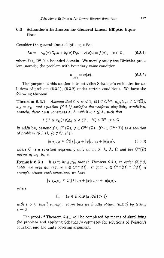
Schauder's Estimates for Linear Elliptic Equations 187
6.3 Schauder's Estimates for General Linear Elliptic Equations
Consider the general linear elliptic equation
Lu = —a,ij(x)DijU + bi(x)DiU + c(x)u = f(x), x € CI, (6.3.1)
where fi c R™ is a bounded domain. We merely study the Dirichlet problem, namely, the problem with boundary value condition
= <p(x). (6.3.2) oil
The purpose of this section is to establish Schauder's estimates for solutions of problem (6.3.1), (6.3.2) under certain conditions. We have the following theorem.
Theorem 6.3.1 Assume that 0 < a < 1, 9 0 6 C2>a, a^^c £ Ca(Tl), aij = aji, and equation (6.3.1) satisfies the uniform ellipticity condition, namely, there exist constants A, A with 0 < A < A, such that
A|£|2 < aijWtej < A|£|2, V£ e l n , i £ 0 .
In addition, assume f £ Ca(fi), </? £ C2'a(Q). Ifu£ C2'a(fl) is a solution of problem (6.3.1), (6.3.2), then
M2,a;ft ^ CG/k f i + M2,a;fi + Mo;fj), (6.3.3)
where C is a constant depending only on n, a, A, A, 0 and the Ca(Cl) norms of'ay, bi, c.
Remark 6.3.1 It is to be noted that in Theorem 6.3.1, in order (6.3.3) holds, we need not require u £ C2'a(fl). In fact, u £ C2'a(Cl) n C(Cl) is enough. Under such condition, we have
|u|2,a;ne < C(\f\a-n + M2,a;fi + W\o;n),
where
Cl£ = {x £ Cl; dist(x, dd) > e}
with e > 0 small enough. From this we finally obtain (6.3.3) by letting e->0.
The proof of Theorem 6.3.1 will be completed by means of simplifying the problem and applying Schauder's estimates for solutions of Poisson's equation and the finite covering argument.
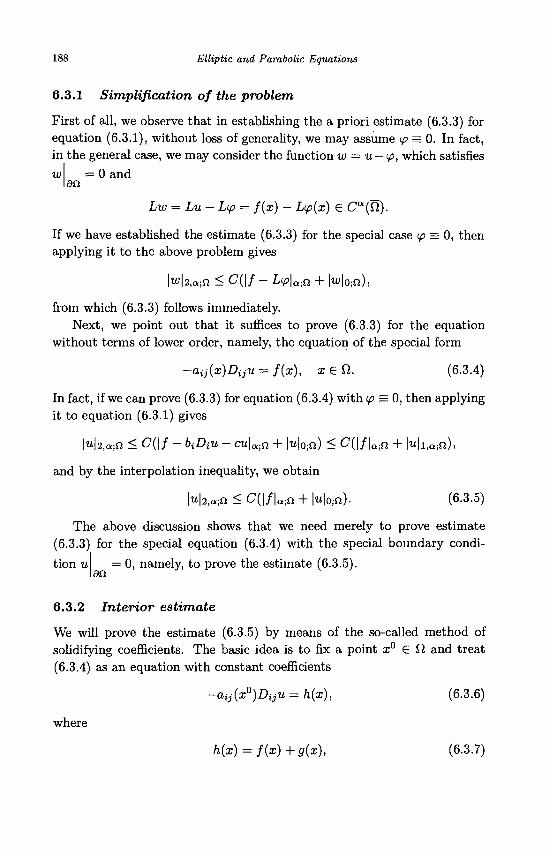
188 Elliptic and Parabolic Equations
6.3.1 Simplification of the problem
First of all, we observe that in establishing the a priori estimate (6.3.3) for equation (6.3.1), without loss of generality, we may assume <p = 0. In fact, in the general case, we may consider the function w = u — (p, which satisfies w = 0 and
an
Lw = Lu-L<p = f(x) - Lip(x) € Ca(Q).
If we have established the estimate (6.3.3) for the special case (p = 0, then applying it to the above problem gives
\w\2,a;Q < C(\f - L(p\a.Q + Mo;fi),
from which (6.3.3) follows immediately. Next, we point out that it suffices to prove (6.3.3) for the equation
without terms of lower order, namely, the equation of the special form
—a,ij(x)DijU — f(x), x £ fi. (6.3.4)
In fact, if we can prove (6.3.3) for equation (6.3.4) with I ^ E O , then applying it to equation (6.3.1) gives
|«|2,ain < C(\f - biDiU - cu\a-a + \u\0.n) < C( | / | a i n + |u|i ,a ;n),
and by the interpolation inequality, we obtain
\u\2,a;U < C(\f\a-Q + |u|o;fi)- (6.3.5)
The above discussion shows that we need merely to prove estimate
(6.3.3) for the special equation (6.3.4) with the special boundary condi
tion u = 0 , namely, to prove the estimate (6.3.5).
6.3.2 Interior estimate
We will prove the estimate (6.3.5) by means of the so-called method of solidifying coefficients. The basic idea is to fix a point x° € fl and treat (6.3.4) as an equation with constant coefficients
—a,ij(x°)DijU = h(x), (6.3.6)
where
h(x) = f(x) + g(x), (6.3.7)
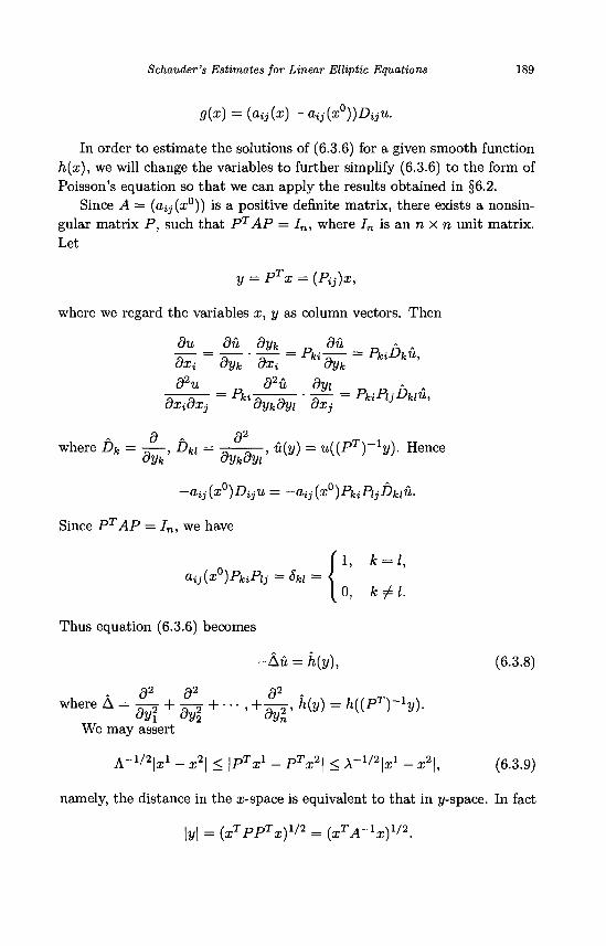
Schauder's Estimates for Linear Elliptic Equations 189
g(x) = (a,ij(x) - aij(x°))DijU.
In order to estimate the solutions of (6.3.6) for a given smooth function h(x), we will change the variables to further simplify (6.3.6) to the form of Poisson's equation so that we can apply the results obtained in §6.2.
Since A = (ciij(x0)) is a positive definite matrix, there exists a nonsin-gular matrix P , such that PTAP — In, where In is an n x n unit matrix. Let
y = PTx = (P^x,
where we regard the variables x, y as column vectors. Then
du du dyk D du D A . dxi dyk dxi dyk
d2u d2u dyi = Pkia.. *.. ' ~^r = PkiPljDklU, dxidxj dykdyi dx
d - d 2
where Dk = — , Dkl = ^ - ^ - , u{y) = u{{PT)-ly). Hence
-a,ij(x0)DijU = -aij{x°)PkiPijbkiu.
Since PTAP = In, we have
ay(a;0)Pfc<Py = 6kl =
Thus equation (6.3.6) becomes
- A n = h(y), (6.3.8)
where A=!*+M+'""'+5rh{y)=K{pT)~ly)-We may assert
A " 1 / V - A < \PTxl - PTx2\ < \~l'2\xl - x2\, (6.3.9)
namely, the distance in the x-space is equivalent to that in y-space. In fact
\y\ = {xTPPTx)x'2 = (xTA~1x)^2.
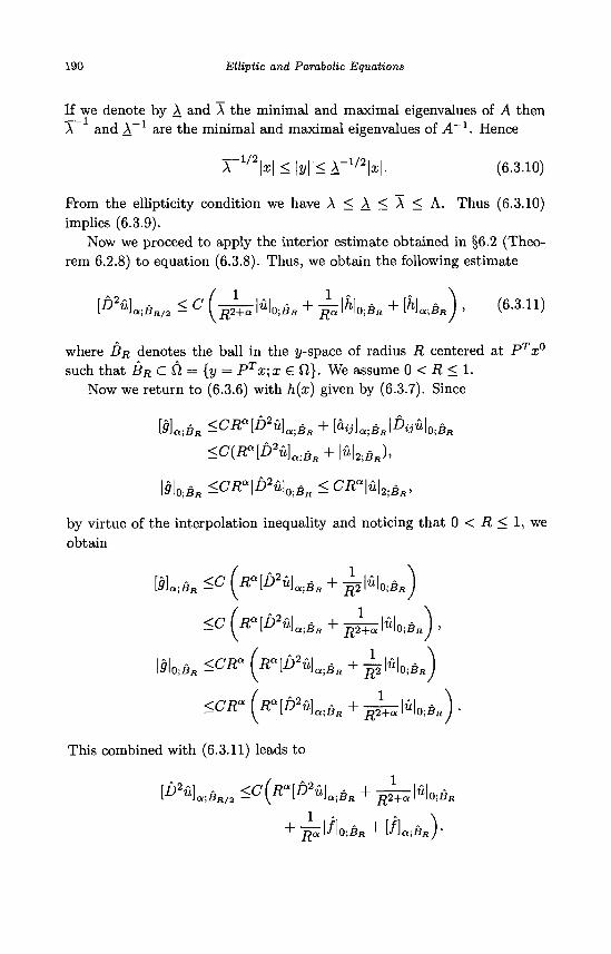
190 Elliptic and Parabolic Equations
If we denote by A and A the minimal and maximal eigenvalues of A then A and A are the minimal and maximal eigenvalues of A~1. Hence
A~ I / 2 |z | < \y\ < A_1 /2 |x|- (6.3.10)
From the ellipticity condition we have A < A < A < A. Thus (6.3.10) implies (6.3.9).
Now we proceed to apply the interior estimate obtained in §6.2 (Theorem 6.2.8) to equation (6.3.8). Thus, we obtain the following estimate
where BR denotes the ball in the y-space of radius R centered at PTx° such that BR C Cl = {y = PTx; x € 9,}. We assume 0 < R < 1.
Now we return to (6.3.6) with h{x) given by (6.3.7). Since
[g]a,BR <CRa[D2u]a,BR + [ f i y U s J A i f i l o ; ^
<C(Ra[D2u}a.>BR + \u\2;BR),
\9\Q]BR<CRa\D2u\0,BR<CRa\u\^BR,
by virtue of the interpolation inequality and noticing that 0 < R < 1, we obtain
[9\a.,BR<c[Ra[D2u]a]BR + ^2\u\o-,BR)
<c(Ra[D2u]a.iBR + ^\u\0.,BR),
\9\0]BR <CR" (Ra[D2u]a;BR + ^\o-,BR)
<CRa[Ra[D2u]a,BR + ^\u\0,BR).
This combined with (6.3.11) leads to
[D2u\a,BR/2 <c(Ra[D2u}a,BR + J^\U\0;BR
+ ~]^\f\o;BR + lf}a;BR)-
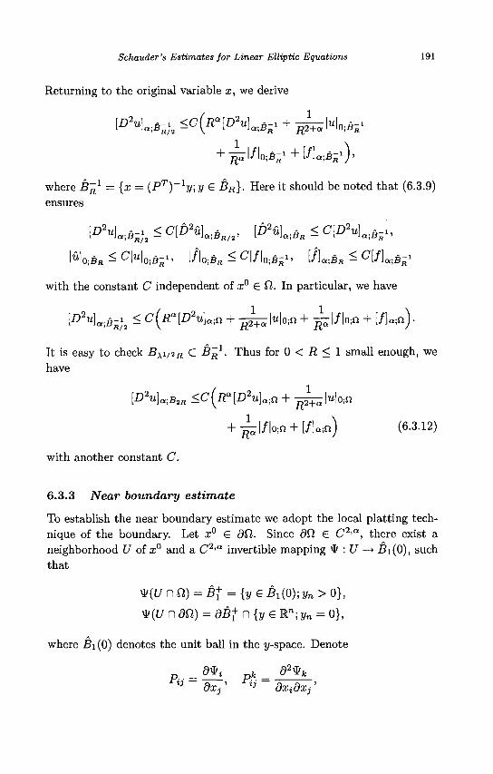
Schauder's Estimates for Linear Elliptic Equations 191
Returning to the original variable x, we derive
where B'1 = {x = (PT)-1y; y € BR}. Here it should be noted that (6.3.9) ensures
No;B„ < C\U\0;B-1, | / |0;B f l < C | / | 0 . B - I , [f]a.6R < C[/]a .B-i
with the constant C independent of x° € fi. In particular, we have
ID2<-,B-}2 < c{Ra[D2u]a.n + ^ M o ; n + ^ | / | o ; n + [/] a in).
It is easy to check Bxi/2R C BR1. Thus for 0 < R < 1 small enough, we have
[D2u]a.B2R <c(Ra[D2u}a;n + ^ > | o ; n
+ ^ l / | o : n + [/]„;n) (6.3.12)
with another constant C.
6.3.3 Near boundary estimate
To establish the near boundary estimate we adopt the local platting technique of the boundary. Let x° e dfl. Since dCl £ C 2 , a , there exist a neighborhood U of x° and a C 2 , a invertible mapping \I> : U —> Bi(0), such that
V(U nf i ) = B+ = {|/e Bi(0); yn > 0},
¥(CA n dQ) = dB+ n {y £ R"; yn = 0},
where Bi(0) denotes the unit ball in the y-space. Denote
p. =d% k d^k 13 BXj' ij dXidXj'
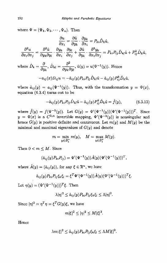
192 Elliptic and Parabolic Equations
where * = (*X) * 2 , • • • , *«)• Then
du du dyk D A . dxi dyk axi
d2u d2u dyk dyi du d2yk - fe " -dxidxj dykdyi dxi dxj dyk dxidxj ° y' '
d - d2
where Dk = -=—, Dki = -—5—, u(y) = u ( * ^j/)). Hence
-aij(x)Diju = -aij(y)PkiPijDkiu - aij(y)PfcjDku,
where a>ij(y) = aij('^~1(y)). Thus, with the transformation y = ^(x), equation (6.3.4) turns out to be
-ai^PkiPijDuu - aij(y)PlcjDkU = f{y), (6.3.13)
where f(y) = / ( * - x ( » ) ) . Let G(y) = * ' (* - 1 (y ) ) (* , (* - 1 ( t f ) ) ) r . Since y = $(x) is a C2'a invertible mapping, \P'(\I>-1(y)) is nonsingular and hence G(y) is positive definite and continuous. Let m{y) and M{y) be the minimal and maximal eigenvalues of G(y) and denote
m = min m(y), M = max M{y). yeB+ y€B+
Then 0 < m < M. Since
(a^PkiPj) = * ' ( * - 1 ( 2 / ) ) i ( 2 / ) ( ^ ( * - 1 ( 2 / ) ) ) T ,
where A(y) = (a,ij(y)), for any £ € Mn, we have
&ij{y)PuPijtei = ^ * ' ( * - 1 ( y ) ) i ( y ) ( * ' ( * - 1 ( y ) ) ) T e
Let 77(2/) = ( ^ ( t f - 1 ^ ) ) ) ^ . Then
AM2 < cuMPkiPiM < A|T?|2.
Since |?y|2 = rjTr] = £,TG(y)£, we have
m|£|2 < H2 < M|£|2.
Hence
Am|£|2 < cuMPkiPiMi < AM|e|2.
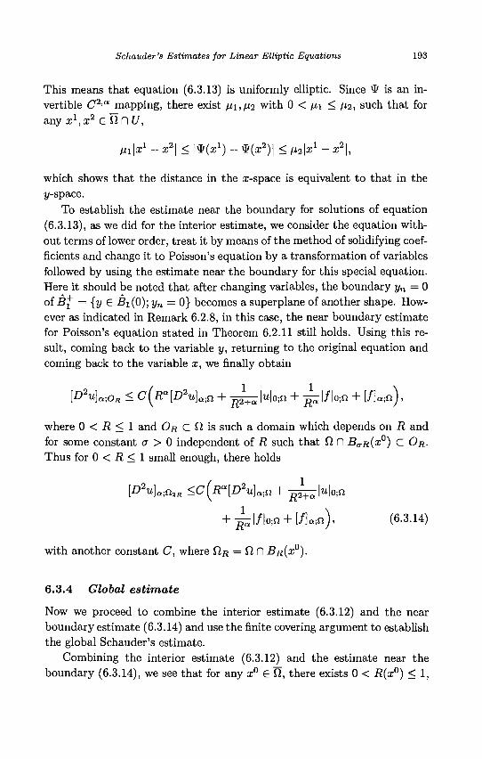
Schauder 's Estimates for Linear Elliptic Equations 193
This means that equation (6.3.13) is uniformly elliptic. Since * is an in-vertible C2'a mapping, there exist /xi,/X2 with 0 < /zi < fi2, such that for any xl,x2 £ ft fl U,
H^x1 - x2\ < |^(xx) - * (x 2 ) | < n2\xl - x2\,
which shows that the distance in the x-space is equivalent to that in the y-space.
To establish the estimate near the boundary for solutions of equation (6.3.13), as we did for the interior estimate, we consider the equation without terms of lower order, treat it by means of the method of solidifying coefficients and change it to Poisson's equation by a transformation of variables followed by using the estimate near the boundary for this special equation. Here it should be noted that after changing variables, the boundary yn = 0 of B± = { ) / £ Bi(0);yn = 0} becomes a superplane of another shape. However as indicated in Remark 6.2.8, in this case, the near boundary estimate for Poisson's equation stated in Theorem 6.2.11 still holds. Using this result, coming back to the variable y, returning to the original equation and coming back to the variable x, we finally obtain
[D2u)a,oR < c(Ra\D2u]a,u + ^ | « | o ; n + ^ l / k n + [/]«.;«),
where 0 < R < 1 and OR C fi is such a domain which depends on R and for some constant a > 0 independent of R such that Q fl BaR(x0) C OR. Thus for 0 < R < 1 small enough, there holds
[D2uUn2R <c(Ra[D2u}a,u + ^ ^ | « | o ; n
+ ^ l / l o ; n + [ / U n ) , (6-3.14)
with another constant C, where CIR = ft n BR(X°).
6.3.4 Global estimate
Now we proceed to combine the interior estimate (6.3.12) and the near boundary estimate (6.3.14) and use the finite covering argument to establish the global Schauder's estimate.
Combining the interior estimate (6.3.12) and the estimate near the boundary (6.3.14), we see that for any x° £ ft, there exists 0 < R(x°) < 1,
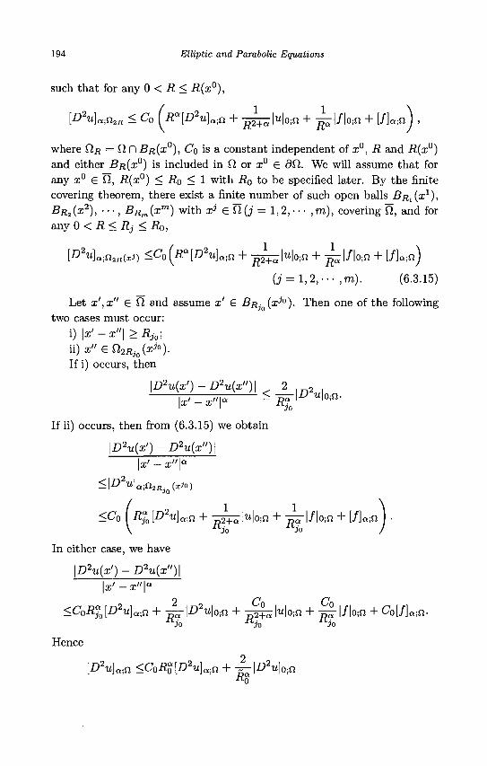
194 Elliptic and Parabolic Equations
such that for any 0 < R < R(x°),
[D2u]a.,n2R < Co (Ra[D2u]a.t(l + ^ | « | 0 i n + ^ l / k n + [/]« ;n) ,
where CIR = fi n BR(X°), CQ is a constant independent of x°, R and R(x°) and either BR(X°) is included in Q or x° e dfl. We will assume that for any x° € fi, i?(x°) < -Ro < 1 with .R0 to be specified later. By the finite covering theorem, there exist a finite number of such open balls BR1(X
1),
BR2 (X2), •••, BRm (xm) with xJ' £ CI (j = 1,2, • • • , m), covering fi, and for any 0 < R < R3 < Ro,
[D2u]a.U2R{xJ) <C0(Ra[D2u]a;Q + ^\u\0-n + ^ | / | 0 i n + IfUn)
(j = l , 2 , - - - , m ) . (6.3.15)
Let x',x" € fi and assume x' G BRJO{X^°). Then one of the following two cases must occur:
i) \x' -x"\ >Rjo; n)x"en2RJ0(xt°). If i) occurs, then
\D2u(x') - D2u(x")\ ^ 2 < -S5-I^«|0 ,n.
•""jo
If ii) occurs, then from (6.3.15) we obtain
\D2u{x') - D2u(x")\
,.,„<**>) <\D2u\a-,n2Rji
<C0 IR%[D2u}a]U + - ^ > | o ; n + ^ r l / l o j n + [ / k n
In either case, we have
\D2u(x') - D2u{x")\
\x' — x"
<C0Rl\D2u]a,u + ~\D2u\0.tQ + 4 ^ > | o ; n + -j§-|/|o ;n + C0[/]Qin. U3o Hj0
KJo
Hence
\D2u}a,n <CQR%[D2u)a.n + S\D2u\o-,a R0
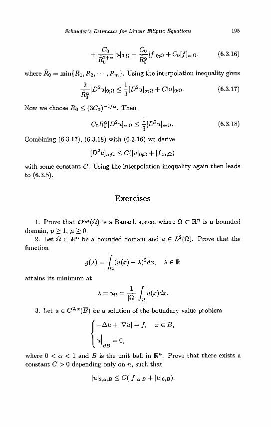
Schauder's Estimates for Linear Elliptic Equations 195
+ W ^ M o s n + S / l c n + CotfUci. (6.3.16)
where Ro = min{.R1, R2, • • • , i? m }. Using the interpolation inequality gives
•§-\D2u\o-,n < \{D2u]a.,ci + C\u\0,n. (6.3.17)
Now we choose Ro < ( 3C 0 ) _ 1 / a . Then
CQRt[D2u\a,Q < ^[D2u]a.,n, (6.3.18)
Combining (6.3.17), (6.3.18) with (6.3.16) we derive
[D2u]a,n < C(|u|0;n + l /Un)
with some constant C. Using the interpolation inequality again then leads to (6.3.5).
Exercises
1. Prove that £p'M(fi) is a Banach space, where Cl C Rn is a bounded domain, p > 1, /x > 0.
2. Let fi C K™ be a bounded domain and u G L2(fi). Prove that the function
g{\) = f {u(x) - X)2dx, X £ Jn
attains its minimum at
x = u^W\iu{x)da \n\
3. Let u £ C2'a(B) be a solution of the boundary value problem
' -Au + \Vu\ = / , x € B,
u = 0, dB
where 0 < a < 1 and B is the unit ball in W1. Prove that there exists a constant C > 0 depending only on n, such that
\u\2,a;B < C{\f\a-,B + |w|o;fi)-
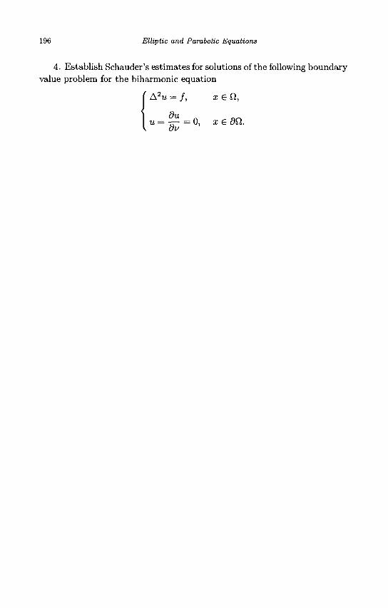
196 Elliptic and Parabolic Equations
4. Establish Schauder's estimates for solutions of the following boundary value problem for the bihaxmonic equation
r A 2U = /, x € Q,
X6ffl .
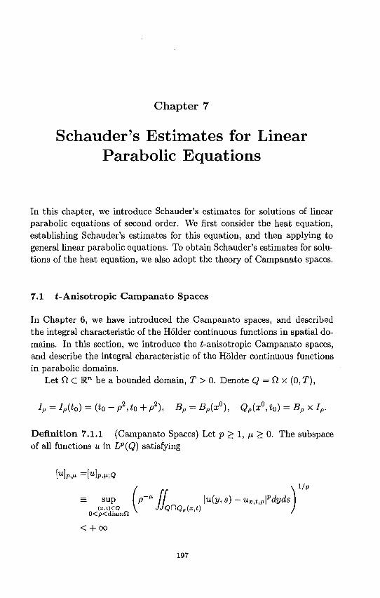
Chapter 7
Schauder's Estimates for Linear Parabolic Equations
In this chapter, we introduce Schauder's estimates for solutions of linear parabolic equations of second order. We first consider the heat equation, establishing Schauder's estimates for this equation, and then applying to general linear parabolic equations. To obtain Schauder's estimates for solutions of the heat equation, we also adopt the theory of Campanato spaces.
7.1 t-Anisotropic Campanato Spaces
In Chapter 6, we have introduced the Campanato spaces, and described the integral characteristic of the Holder continuous functions in spatial domains. In this section, we introduce the ^-anisotropic Campanato spaces, and describe the integral characteristic of the Holder continuous functions in parabolic domains.
Let Q C R" be a bounded domain, T > 0. Denote Q = £1 x (0,T),
Ip = IP{to) = {to-p2,t0 + p2), Bp = Bp(x°), Qp{x°,t0) = BpxIp.
Definition 7.1.1 (Campanato Spaces) Let p > 1, n > 0. The subspace of all functions u in LP(Q) satisfying
MP,M =[U1P,M;Q
= sup \P~ti \u(y,s)-uXit,P\pdyds) (x,t)£Q \ JJQC\QJx,t) I
< + 00
197
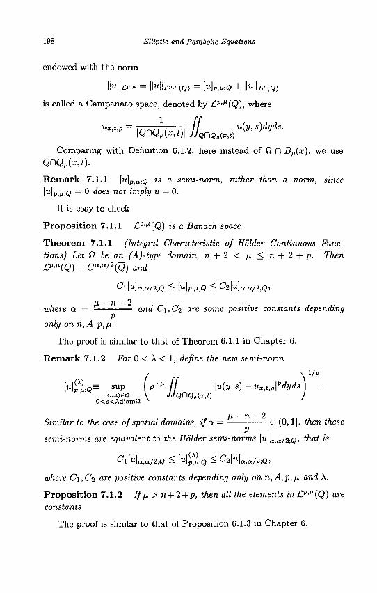
198 Elliptic and Parabolic Equations
endowed with the norm
||w|U».e = IMUP.M(Q) = M P I M ; Q + ||U||LP(Q)
is called a Campanato space, denoted by £P,M(Q), where
"*•*•' = \nnn (n- *\\ II " ^ ' s)dVds-
Comparing with Definition 6.1.2, here instead of fi n Bp(x), we use QnQp(x,t).
R e m a r k 7.1.1 [u]p,/i;Q is a semi-norm, rather than a norm, since [U\P,IJ,;Q — 0 does not imply u = 0.
It is easy to check
Proposi t ion 7.1.1 £P'M(Q) is a Banach space.
Theorem 7.1.1 (Integral Characteristic of Holder Continuous Functions) Let fi be an (A)-type domain, n + 2 < /x < n + 2 + p. Then £p."(Q) = Ca'a/2(Q) and
Cl[u]ata/2,Q < [u]p,n,Q < C 2 M a , a / 2 , Q )
where a = and C\, C2 are some positive constants depending P
only on n,A,p,fi.
The proof is similar to that of Theorem 6.1.1 in Chapter 6.
R e m a r k 7.1.2 For 0 < A < 1, define the new semi-norm
MJ2;Q= S U P (P~* II l«(y.s) ~ ux,t,P\pdyds I . (x.oeq V JJQC\Qp(x,t) )
0<p<Adiamn X '
Similar to the case of spatial domains, ifa= € (0,1], then these
semi-norms are equivalent to the Holder semi-norms [u]a,a/2;Q, that is
ClMa,a/2;Q < Mp^;Q ^ C2{u)a^/2-Q,
where C\,C2 are positive constants depending only on n,A,p,fi and X.
Proposi t ion 7.1.2 If fi> n + 2+p, then all the elements in Cp,tl(Q) are constants.
The proof is similar to that of Proposition 6.1.3 in Chapter 6.
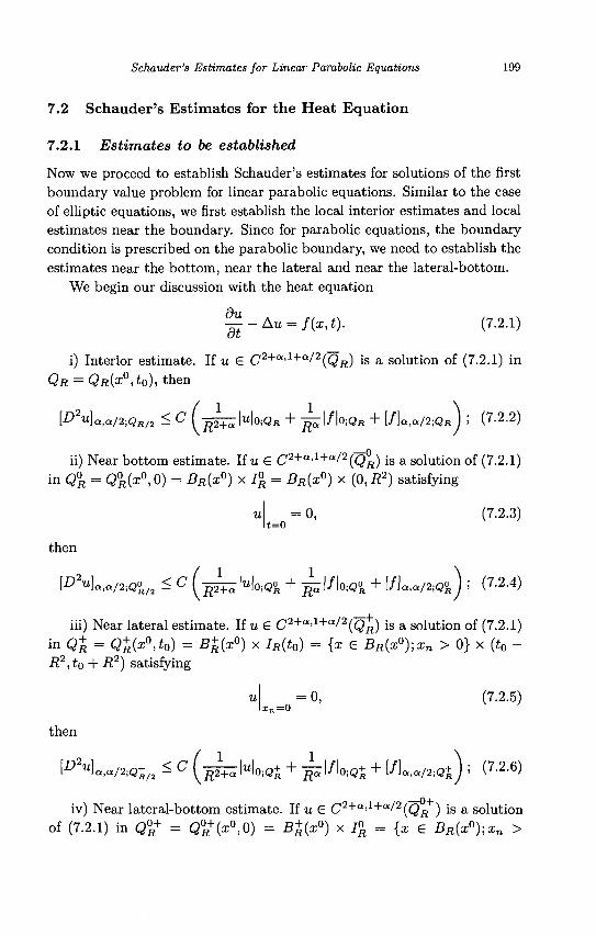
Schauder's Estimates for Linear Parabolic Equations 199
7.2 Schauder's Estimates for the Heat Equation
7.2.1 Estimates to be established
Now we proceed to establish Schauder's estimates for solutions of the first boundary value problem for linear parabolic equations. Similar to the case of elliptic equations, we first establish the local interior estimates and local estimates near the boundary. Since for parabolic equations, the boundary condition is prescribed on the parabolic boundary, we need to establish the estimates near the bottom, near the lateral and near the lateral-bottom.
We begin our discussion with the heat equation
^ - A u = f(x,t). (7.2.1)
i) Interior estimate. If u G C2+a'1+a/2(QR) is a solution of (7.2.1) in
QR = QR{XQM), then
\D2u]aia/2.QR/2 < C (jl^\u\0.QK + ^ l / l o i Q * + [ / ] a , « / 2 ; Q B ) I (7-2.2)
ii) Near bottom estimate. If u € C2+a<1+a/2(cfR) is a solution of (7.2.1) in Q°R = Q°R(x°,0) = BR(x°) xI°R = BR{x°) x (0,R2) satisfying
= 0, (7.2.3) t=o
then
[D2u}a,a/2]Q0R/2 < C ( ^ M o ; Q ° R + ^l/l0;QOR + [f\a,a/2&^ ! (7-2.4)
iii) Near lateral estimate. If u e C 2 + a ' 1 + Q / 2 (Q^) is a solution of (7.2.1) in Q+ = Q+(xVo) = B+(x°) x IR(t0) = {x € BR(x°);xn > 0} x (t0 -R2,t0 + R2) satisfying
= 0, (7.2.5) x„=0
then
[D2u]a,a/2.iQ+R/2 < C ( ^ N c o j + ^ 1 / l o i Q j + t / U / a , g j ) 5 (7-2-6)
iv) Near lateral-bottom estimate. If u e C2+a'1+a/2(QR ) is a solution of (7.2.1) in Q°+ = Q°R
+(x°,0) = B+(x°) x 7° = {x e BR(x°);xn >
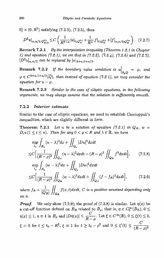
200 Elliptic and Parabolic Equations
0} x (0,i?2) satisfying (7.2.3), (7.2.5), then
^ ] a , a / 2 ^ 2 < ^ ( ^ k l o ; Q O R + + ^ | / | 0 l Q 0 B + + [/]a,Q/2;Q0R+) . (7.2.7)
R e m a r k 7.2.1 By the interpolation inequality (Theorem 1.2.1 in Chapter 1) and equation (7.2.1), we see that in (7.2.2), (7.2.4), (7.2.6) and (7.2.7), [D2u]a^/2 can be replaced by |u|2+a,i+a/2-
R e m a r k 7.2.2 If the boundary value condition IS 111 — {Q CLTld _ dPQ
ip € C2+a'1+a/2(Q), then instead of equation (7.2.1), we may consider the equation for u — tp.
R e m a r k 7.2.3 Similar to the case of elliptic equations, in the following arguments, we may always assume that the solution is sufficiently smooth.
7.2.2 Interior estimate
Similar to the case of elliptic equations, we need to establish Caccioppoli's inequalities, which are slightly different in form.
Theorem 7.2.1 Let u be a solution of equation (7.2.1) in QR, W = DiU (1 < i < n). Then for any 0 < p < R and A £ R, we have
sup / (u — X)2dx + / / \Du\2dxdt h JB„ JJQP
<C []_ (j (u- Xfdxdt + (R- p)2 ff f2dxdt\, (7.2.8)
s u p / (w-X)2dx+ \Dw\2dxdt IP JBf, JjQp
<C[ * jj (w - Xfdxdt + Jj (f - fR)2dxdt], (7.2.9)
where / H = / / f(x, t)dxdt, C is a positive constant depending only \QR\ JJQR
on n.
Proof. We only show (7.2.9); the proof of (7.2.8) is similar. Let r](x) be a cut-off function defined on BR related to Bp, that is, 77 £ CQ°(BR), 0 <
n T](x) < 1, r) = 1 in Bp and \Dr)(x)\ < . Let f £ C°°(R), 0 < £(t) < 1,
R — p (j
£ = 0 for t < t0 - R2, £ = 1 for t > t0 - p2 and 0 < £'(£) < — r? . (H - py
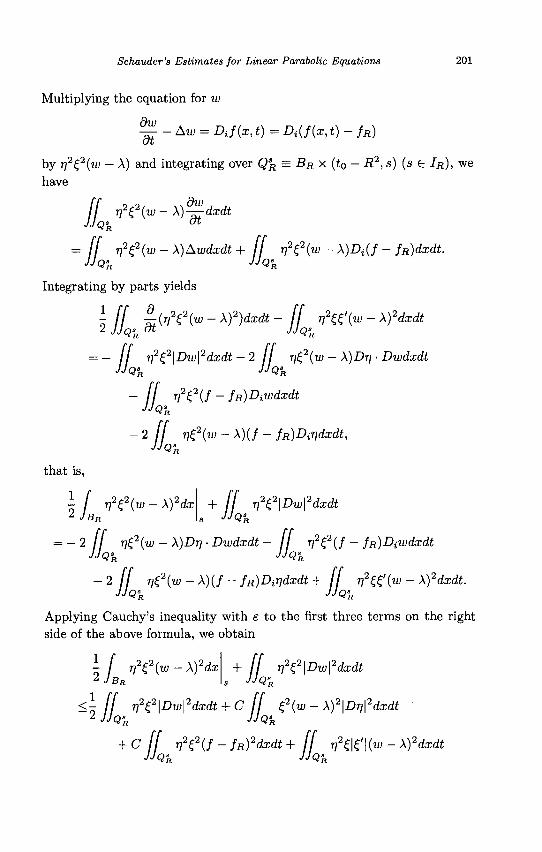
Schauder's Estimates for Linear Parabolic Equations 201
Multiplying the equation for w
^ - AW = DJ(x,t) = Di{f(x,t) - fR)
by r]2t,2(w - A) and integrating over Q3R = BRx (t0 - R2, s) (s € IR), we
have
#,<'« ,<"-*>!?*•* / / V2^2(w - X)Awdxdt + ff r)2Z2(w - X)Di(f - fR)dxdt.
Integrating by parts yields
\ l l itfe{w-\)2)dxdt- ff rftfiw-Xfdxdt 2 JJQR at JJQR
= - ff T]2£2\Dw\2dxdt-2 ff r)Z2(w-\)Dr)-Dwdxdt JJQ'R JJQ'R
- ff r?eU - fR)DiWdxdt JJQ%
-2 ff r)Z2(w - X)(f - fR)DiT]dxdt, JJQ%,
that is,
\f 7]2^2{w-X)2dx + ff r)2£2\Dw\2dxdt 2 JBR S JJQR
= -2 ff ri£2(w-X)Dri-Dwdxdt- ff r)2£2(f - fR)Diwdxdt JjQR JjQn
- 2 ff tf2(w - A)(/ - fR)Dir]dxdt + ff r]2^'(w - X)2dxdt. JJQR JJQR
Applying Cauchy's inequality with e to the first three terms on the right side of the above formula, we obtain
\ f V2Z2(w - A)2dx + ff T]2t2\Dw\2dxdt 2 JBR S JJQR
<\ ff r)2£2\Dw\2dxdt + C ff £,2{w-X)2\Dr)\2dxdt 2 JJQR JJQH
+ C ff V2e(f-fR)2dxdt+ ff r,2£\e\(w - Xfdxdt
JJQ%, JJQ'v
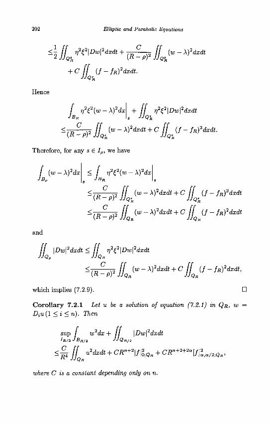
202 Elliptic and Parabolic Equations
4 I. ^ M " * * + Jf (» - A)'** 'Ok
+ cJJa(f-fR)2dxdt.
Hence
dxdt
<
f r,2e(w - \)2dx + ff V2e\Dw\'-
JBR S JJQR
C ff (w- Xfdxdt + C ff (/ - fRf :(R-P)2JJQR
Therefore, for any s e Ip, we have
dxdt.
f (w-X)2dx < f r,2£2(w-X)2dx JB„ S JBR S
-JiSw II .{w ~ x)2dxdt + c II .(/ " fRfdxdt >Q'n
<,RC_ )2 JJ (w-X)2dxdt + C Jf (f-fR)2dxdt
and
/ / \Dw\2dxdt < ff rj2(,2\Dw\: dxdt
<-C ff (w - Xfdxdt + C II (/ - fR)2dxdt,
JJQR JJQR :(R-P)2JJQR
which implies (7.2.9). •
Corollary 7.2.1 Let u be a solution of equation (7.2.1) in QR, w = Diu{l <i<n). Then
sup / w2dx + / / \Dw\2dxdt IR/2 J BR/2 JJQR/2
~W HQR UHXdt + CRn+2W^« + CRn+2+2aVta/2;QR'
where C is a constant depending only on n.
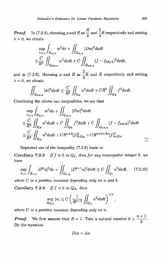
Schauder's Estimates for Linear Parabolic Equations 203
7? "i
Proof. In (7.2.9), choosing p and R as — and -R respectively and setting
A = 0, we obtain
sup / w 2dx + / / \Dw\2dxdt IR/2 •> BR/2 JJQR/2
<•£ / / w2dxdt + C ff (/ - hR/i)2dxdt,
'Q3H/4 JJQsR/i
3 and in (7.2.8), choosing p and R as -R and i? respectively and setting A = 0, we obtain
/ / \w\2dxdt < - ^ / / u2dxdt + CR2 ff fdxdt. JJQ3R/4 R JJQR JJQR
Combining the above two inequalities, we see that
sup / w2dx + / / \Dw\2dxdt IR/2 JBR/2 JJQR/2
< • £ / / u2dxdt + C [[ fdxdt + C ff (f - hn/ifdxdt R JJQR JJQR JJQ3R/4
< £ ff u2dxdt + CR«+2\f\2;QR + CR^2^[f}2
a,QR. n JJQR •
Repeated use of the inequality (7.2.8) leads to
Corollary 7.2.2 If f = 0 in Q\, then for any nonnegative integer k, we have
s u p / \Dku\2dx+ ff \Dk+1u\2dxdt<C ff u2dxdt, (7.2.10) h/2 JB1/2 JJQI/2 JJQI
where C is a positive constant depending only on n and k.
Corollary 7.2.3 If f = 0 in QR, then
izM-c(^ILu2dxdt) ' where C is a positive constant depending only on n.
n + 1 Proof. We first assume that R = 1. Take a natural number k > —-—.
By the equation
Dtu = Au
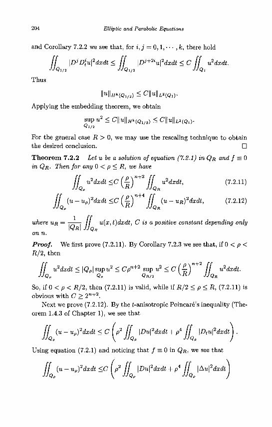
204 Elliptic and Parabolic Equations
and Corollary 7.2.2 we see that, for i, j = 0,1, • • • , k, there hold
ff \DjD\u\2dxdt < ff \Dj+2iu\2dxdt <C ff u2dxdt. JJQI/2 JjQl/2 JJQl
Thus
ll«llff*(Q1/a) < C| |u| |LaW l ) .
Applying the embedding theorem, we obtain
sup u2 < C\\U\\HH{QI/2) < C||u||L2Wl). Q l / 2
For the general case R > 0, we may use the rescaling technique to obtain the desired conclusion. •
Theorem 7.2.2 Let u be a solution of equation (7.2.1) in QR and f = 0 in QR. Then for any 0 < p < R, we have
ff u2dxdt <C ( 4 ) " + / / u2dxdt, (7.2.11)
ff (u-Up)2dxdt<c(^Y+ ff (u-uR)2dxdt, (7.2.12)
where UR = -r-pr—r / / u(x, t)dxdt, C is a positive constant depending only \QR\ JJQR
on n.
Proof. We first prove (7.2.11). By Corollary 7.2.3 we see that, if 0 < p < R/2, then
/ / u2dxdt <\QP\ supu2 < Cpn+2 sup u2 < C (^Y ff u2dxdt. JJQ,, Qp QR/2 K R / JJQR
So, if 0 < p < R/2, then (7.2.11) is valid, while if R/2 < p < R, (7.2.11) is obvious with C > 2n+2.
Next we prove (7.2.12). By the ^-anisotropic Poincare's inequality (Theorem 1.4.3 of Chapter 1), we see that
/ / (u - Upfdxdt <C\p2 ff \Du\2dxdt + p4 / / \Dtu\2dxdt ) .
Using equation (7.2.1) and noticing that / = 0 in QR, we see that
ff (u - up)2dxdt <C Ip2 ff \Du\2dxdt + p4 ff \Au\2dxdt)
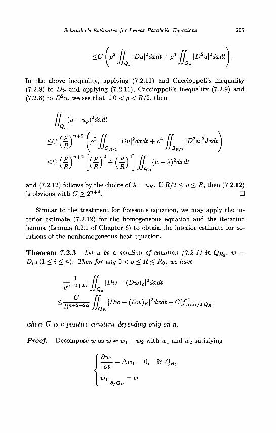
Schauder's Estimates for Linear Parabolic Equations 205
<C\p2 ff \Du\2dxdt + p4 ff \D2u\ \ JJQf, JJQf,
2dxdt .
In the above inequality, applying (7.2.11) and Caccioppoli's inequality (7.2.8) to Du and applying (7.2.11), Caccioppoli's inequality (7.2.9) and (7.2.8) to D2u, we see that if 0 < p < R/2, then
JJQP
up)2dxdt
2dxdt + p4 II \D2u\2dxdt QR/2 J
^(r+2[(i)2+(i)li<«->^ and (7.2.12) follows by the choice of A = uR. If R/2 < p < R, then (7.2.12) is obvious with C > 2"+4. •
Similar to the treatment for Poisson's equation, we may apply the interior estimate (7.2.12) for the homogeneous equation and the iteration lemma (Lemma 6.2.1 of Chapter 6) to obtain the interior estimate for solutions of the nonhomogeneous heat equation.
T h e o r e m 7.2.3 Let u be a solution of equation (7.2.1) in QR0, W = DiU (1 < i < n). Then for any 0 < p < R < RQ, we have
T ^ i i \Dw-(Dw)p\2dxdt
JJQP
ff \Dw - (Dw)R\2dxdt + C\f\2a>a/2iQR,
JJQR
<-C
: Rn+2+2a
where C is a positive constant depending only on n.
Proof. Decompose w as w = w\ + W2 with w\ and w2 satisfying
dt
W\
- Awi = 0, in QR,
dpQR = w
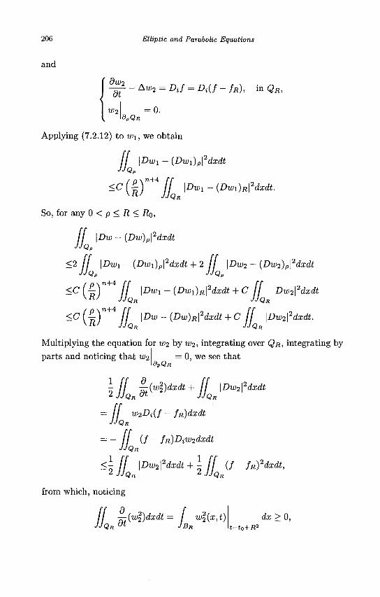
206 Elliptic and Parabolic Equations
and
-^1-Aw2 = DJ = Dt(f - f R ) , in QR,
W2 = 0. dpQn
Applying (7.2.12) to w\, we obtain
/ / \Dwx - (Dwi)p\2dxdt
JJQP
<C ( | ) " + 4 jj \Dw! - (DWl)R\2dxdt.
So, for any 0 < p < R < Ro,
/ / \Dw - {Dw)p\2dxdt
JJQP
<2 / / \Dwi - {Dw{)p\2dxdt + 2 if \Dw2 - (Dw2)p\
2dxdt JJQP JJQ„
<C ( - | ) " + 4 ff \Dw! - (DWl)R\2dxdt + C ff \Dw2\2dxdt
-C{^Y+ ff \Dw-(Dw)n\2dxdt + c ff \Dw2\2dxdt.
Multiplying the equation for w2 by w2, integrating over QR, integrating by
parts and noticing that w2 9VQR
0, we see that
\jjJ-{wl)dxdt + jjjDw. •• II w2Di{f - fR)dxdt JJQR
dxdt
iW2dxdt = - II (/ - /*)At JJQR
<\ jj \Dw2\2dxdt + \ ff (f-fR)2dxdt,
1 JJQR l JJQR
from which, noticing
/ / —{wl)dxdt= I wl(x,t) JJQR ot JBR
dx>0, t=t0 + R2
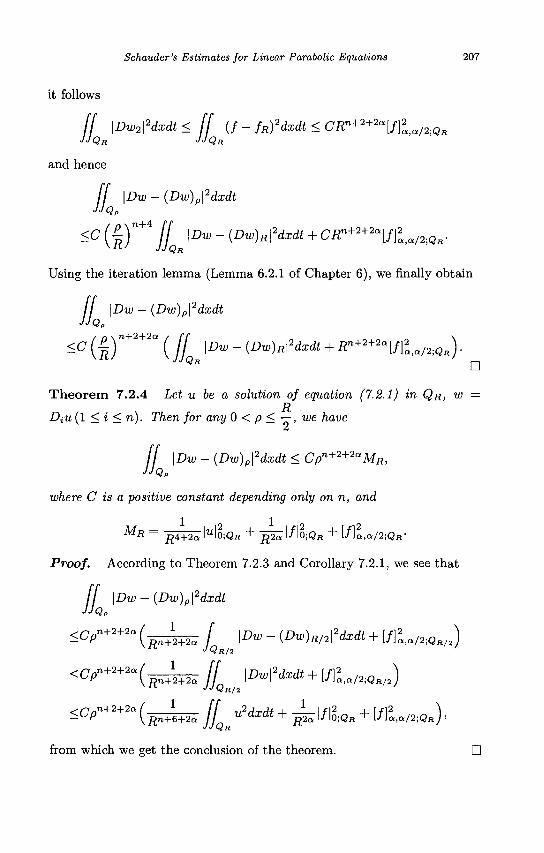
Schauder's Estimates for Linear Parabolic Equations 207
it follows
ff \Dw2\2dxdt < ff (/ - fRfdxdt < CRn+2+2a[f}la/2]QR
JJQR JJQR
and hence
/ / \Dw - (Dw)p\2dxdt
JJQP
<C ( | ) " + 4 JJ \Dw - (Dw)R\2dxdt + CRn+2+2a[f}la/2.<QR.
Using the iteration lemma (Lemma 6.2.1 of Chapter 6), we finally obtain
/ / \Dw- {Dw)p\2dxdt
JJQP
-C(R)n+2+2a(JI \Dw-(Dw)R\2dxdt + R^2+2a[f]la/2.iQR).
Theorem 7.2.4 Let u be a solution of equation (7.2.1) in QR, W =
DiU (1 < i < n). Then for any 0 < p < —-, we have
ff \Dw - (Dw)p\2dxdt < Cpn+2+2aMR,
JJQP
where C is a positive constant depending only on n, and
MR = #4+2a MO;QH + ^2^l/lo ;QR + [f]a,a/2;QR-
Proof. According to Theorem 7.2.3 and Corollary 7.2.1, we see that
/ / \Dw - (Dw)p\2dxdt
JJQP
<CPn+2+2a ( ^ ^ / \Dw - (Dw)R/2\
2dxdt + [f)l,a/2;QR/2)
<CPn+2+2a ( — ^ ff \Dw\2dxdt + [f]l>a/2.iQR/2)
•"• JJQR/2
<CPn+2+2a(—^ JJQR u2dxdt + \f\2
0]QR + Wl,a/*QR).
from which we get the conclusion of the theorem. •
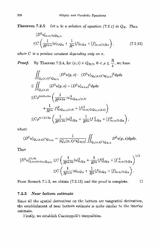
208 Elliptic and Parabolic Equations
Theorem 7.2.5 Let u be a solution of equation (7.2.1) in QR. Then
[D2u}a,a,2;QR/2
^C ( # T ^ M o ; Q « + Jfi\f\o;Qn + I/]<W2;Q*) , (7-2.13)
where C is a positive constant depending only on n.
Proof. By Theorem 7.2.4, for (x,t) e QR/2, 0 < p < —, we have
/ / \D2u{v,«) - (D2u)Qp{Xtt)nQ \2dyds JJQp(x,t)f]QR/2
< ff \D2u(y, s) - (D2u)XttJ2dyds
JJQp(x,t)
</n. n+2+2a ( 1 I |2 I i?4+2alUIO;QR / 2(x, t)
+ jR2Sn/ '0iQR /2(i , t ) + l / Ja ,a /2;Q f i / 2 (x , t ) J
<C/Jn + + " ( ^ 4 + 2 Q I U I O ; Q B + ^ ^ l / l o ; Q H + [f]a,a/2;QRJ >
where
Thus
1/2
[-0 U ]2 ,n+2+2a ;Q R / 2 ^ ^ (p4+2c« lU lo;QR + £ 2 ^ l / l o ; Q H + [ / ]a ,a /2 ;Q R
- ^ ( ^2+^l" l°^« + ^ I ^ I ° ; Q R + [f\a,a/2;QR ) •
Prom Remark 7.1.2, we obtain (7.2.13) and the proof is complete. •
7.2.3 Near bottom estimate
Since all the spatial derivatives on the bottom are tangential derivatives, the establishment of near bottom estimate is quite similar to the interior estimate.
Firstly, we establish Caccioppoli's inequalities.
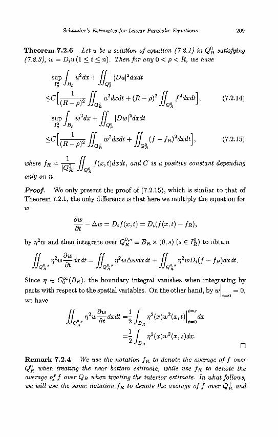
Schauder's Estimates for Linear Parabolic Equations 209
Theorem 7.2.6 Let u be a solution of equation (7.2.1) in QR satisfying (7.2.3), w = Dtu (1 < i < n). Then for any 0 < p < R, we have
sup / u2dx + / / \Du\2dxdt i° JBP JJQO
sup / w2dx + / / \Dw\2dxdt JB„ JJQ°
<C (7.2.14)
i°P JBD
, p 1
s2 / / w2dxdt+ [[ (f - fR)2dxdt\, (7.2.15) {R - pY JJQOR JJQ0R J
where fn = 0 / / f(x, t)dxdt, and C is a positive constant depending \QR\ JJQI
only on n.
Proof. We only present the proof of (7.2.15), which is similar to that of Theorem 7.2.1, the only difference is that here we multiply the equation for w
dw ~dt
- Aw = Dif(x,t) = Di(f(x,t) - f R ) ,
by r)2w and then integrate over Q^8 = BR X (0, s) (s € IR) to obtain
/ / ri2w-pr- dxdt = II ri2wAwdxdt+ / / tfwDAf — fn)dxdt. JJQ°-° ot JJQo,s JJQO,S iQr >QT
Since rj e CQ°(BR), the boundary integral vanishes when integrating by
parts with respect to the spatial variables. On the other hand, by w
we have t=o = 0,
UQR, f^dxdt =\ j ^ rj2(x)w2(x,t) t=s
dx t=o
4/./w w2(x, s)dx.
D
Remark 7.2.4 We use the notation f& to denote the average of f over QR when treating the near bottom estimate, while use fR to denote the average of f over QR when treating the interior estimate. In what follows, we will use the same notation fR to denote the average of f over Q^ and
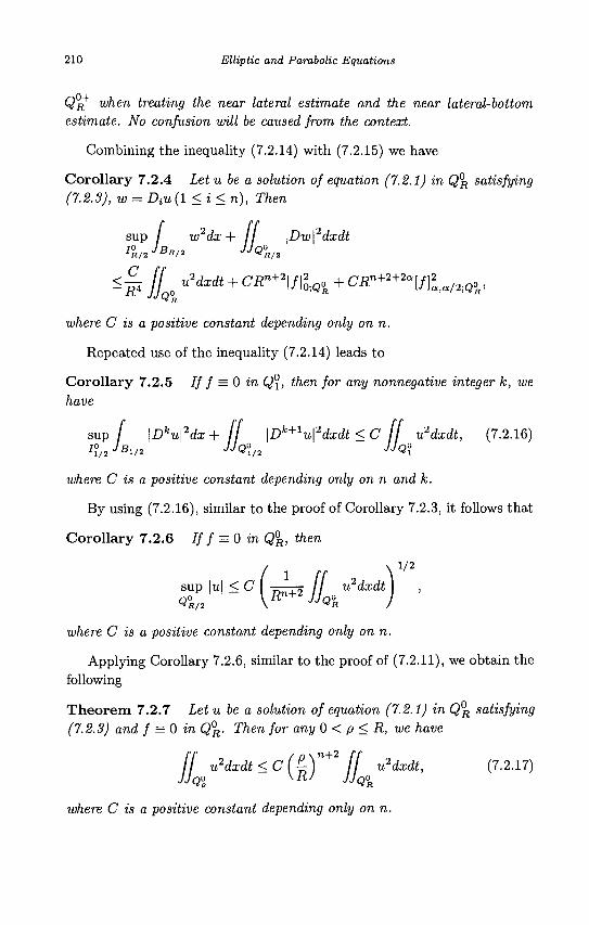
210 Elliptic and Parabolic Equations
QR when treating the near lateral estimate and the near lateral-bottom estimate. No confusion will be caused from the context.
Combining the inequality (7.2.14) with (7.2.15) we have
Corollary 7.2.4 Letu be a solution of equation (7.2.1) in Q°R satisfying (7.2.3), w = Diu(l <i<n), Then
sup / w2dx + / / \Dw\2dxdt i°R/2 JBR/2 JJQ°R/2
~W II o uHxdt + CSr*2W*«k + CRn+2+2aWl«,2;Q°R>
where C is a positive constant depending only on n.
Repeated use of the inequality (7.2.14) leads to
Corollary 7.2.5 If f = 0 in Q\, then for any nonnegative integer k, we have
s u p / \Dku\2dx+ ff \Dk+1u\2dxdt < C ff u2dxdt, (7.2.16) n/2 JBU2 JJQ°1/2 JJQ\
where C is a positive constant depending only on n and k.
By using (7.2.16), similar to the proof of Corollary 7.2.3, it follows that
Corollary 7.2.6 If f = 0 in Q°R, then
( \ 1 / 2
sup H < C I -^-To / / u2dxdt 1 Q%, \ R + JJQ°n J
where C is a positive constant depending only on n.
Applying Corollary 7.2.6, similar to the proof of (7.2.11), we obtain the following
Theorem 7.2.7 Let u be a solution of equation (7.2.1) in QR satisfying (7.2.3) and f = 0 in Q°R. Then for any 0 < p < R, we have
ff u2dxdt<c(^-)n+ ff u2dxdt, (7.2.17) JJQO \R; JJQOR
where C is a positive constant depending only on n.
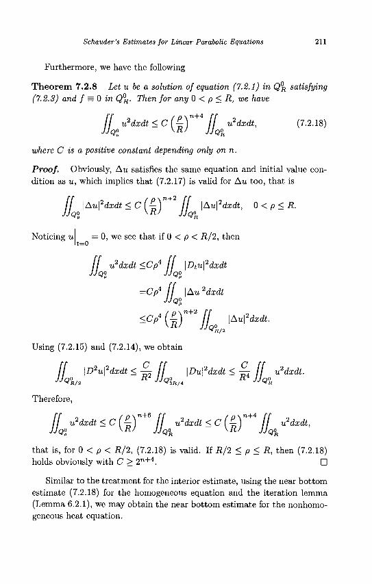
Schauder 's Estimates for Linear Parabolic Equations 211
Furthermore, we have the following
Theorem 7.2.8 Let u be a solution of equation (7.2.1) in Q°R satisfying (7.2.3) and f = 0 in QR. Then for any 0 < p < R, we have
II u2dxdt<c(J^\n+ I] u2dxdt, (7.2.18)
where C is a positive constant depending only on n.
Proof. Obviously, Au satisfies the same equation and initial value condition as u, which implies that (7.2.17) is valid for Aw too, that is
/ / \Au\2dxdt<c(^-)n+ ff \Au\2dxdt, 0 < p < R. JJQO \RS JJQOR
Noticing u = 0, we see that if 0 < p < R/2, then t=o
/ / u2dxdt <Cp4 [[ \Dtu\2dxdt JJQ° JJQ0,
=Cpi ff \Au\2dxdt JJQ°P
Using (7.2.15) and (7.2.14), we obtain
/ / \D2u\2dxdt <—r ff \Du\2dxdt < — f u2dxdt. JJQ%, R JJQ%R/i
R JJQ°R
Therefore,
ff u2dxdt<C^Y+6 ff u2dxdt<c(^Y+i ff u2dxdt,
that is, for 0 < p < R/2, (7.2.18) is valid. If R/2 < p < R, then (7.2.18) holds obviously with C > 2"+4. •
Similar to the treatment for the interior estimate, using the near bottom estimate (7.2.18) for the homogeneous equation and the iteration lemma (Lemma 6.2.1), we may obtain the near bottom estimate for the nonhomo-geneous heat equation.
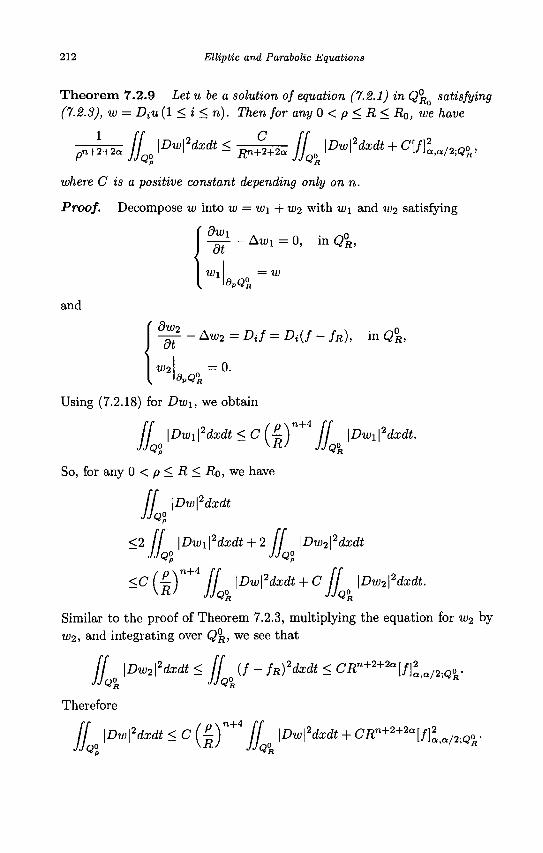
212 Elliptic and Parabolic Equations
Theorem 7.2.9 Let u be a solution of equation (7.2.1) in QR satisfying (7.2.3), w = DiU (1 < i < n). Then for any 0 < p < R < RQ, we have
- ^ Ij^ \Dw\2dxdt < ^ ^ Jl^ \DW\2dxdt + C[/]2Q,a/2;QoR,
where C is a positive constant depending only on n.
Proof. Decompose w into w = w\ + W2 with w\ and w2 satisfying
- B - - Awi = 0, in Q°R,
Wl Wh
w
and
f ^ - Aw2 = DJ = A ( / - / « ) , ™Q%
W2 0. 9PQ°R
Using (7.2.18) for Dw\, we obtain
/ / \DWl\2dxdt<c(^]n+ ff \DWl\
2dxdt. JJQO \R/ JJQ<R
So, for any 0 < p < R < Ro, we have
/ / \Dw\2dxdt
<2 / / \Dw1\2dxdt + 2 / / \Dw2\
2dxdt JJQ° JJQ°P
<c(^)n+A jl \Dw\2dxdt + C ff \Dw2\2dxdt.
KRJ JJQR JJQl
Similar to the proof of Theorem 7.2.3, multiplying the equation for w2 by w2, and integrating over QR, we see that
ff \Dw2\2dxdt < ff ( / - fR)2dxdt < CRn+2+2a[f}2
aiOc/2.iQ0R. >QH
Therefore
II o \Dw\2dxdt < C ( £ ) " + 4 IIQ \Dw\2dxdt + CRn+2+2a[f}2ata/2.iQoR.
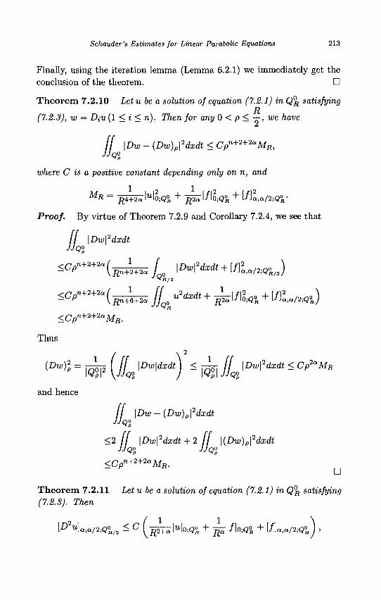
Schauder's Estimates for Linear Parabolic Equations 213
Finally, using the iteration lemma (Lemma 6.2.1) we immediately get the conclusion of the theorem. D
Theorem 7.2.10 Let u be a solution of equation (7.2.1) in Q°R satisfying
(7.2.3), w = DiU (1 < i < n). Then for any 0 < p < —, we have
II \Dw - (Dw)p\2dxdt < Cpn+2+2aMR,
JJQ°
where C is a positive constant depending only on n, and
MR = flS+^Ho;^ + ^ l / l o ; Q ^ + U\l,a/2;QR-
Proof. By virtue of Theorem 7.2.9 and Corollary 7.2.4, we see that
/ / \Dw\2dxdt Hs p
^pn+2+2a ( ^ W L u 2 d x d t + ^ ^ + [ / 1 - / ^ 0 <Cpn+2+2aMR.
Thus
{D< - w? [L | D«"H£ m IL |D""2<fa<" - CI?"MR
and hence
/ / \Dw - {Dw)p\2dxdt
JJQ°P
<2 II \Dw\2dxdt + 2 II \(Dw)p\2dxdt
JJQ° JJQ°P
<Cpn+2+2aMR.
Theorem 7.2.11 Let u be a solution of equation (7.2.1) in QR satisfying (7.2.3). Then
[D2u}ata/2.Q°R/2 < C ^-^2T^Mo;Q°„ + -jp\f\o;Q°R + lf}a,a/2;QR) >
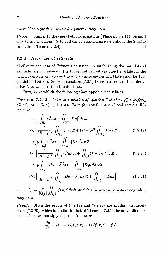
214 Elliptic and Parabolic Equations
where C is a positive constant depending only on n.
Proof. Similar to the case of elliptic equations (Theorem 6.2.11), we need only to use Theorem 7.2.10 and the corresponding result about the interior estimate (Theorem 7.2.4). •
7.2.4 Near lateral estimate
Similar to the case of Poisson's equation, in establishing the near lateral estimate, we can estimate the tangential derivatives directly, while for the normal derivatives, we need to apply the equation and the results for tangential derivatives. Since in equation (7.2.1) there is a term of time derivative Dtu, we need to estimate it too.
First, we establish the following Caccioppoli's inequalities.
Theorem 7.2.12 Letu be a solution of equation (7.2.1) in Q\ satisfying (7.2.5), w = DiU (1 < i < n). Then for any 0 < p < R and any A e E", we have
sup / u2dx + / / \Du\2dxdt iP JB+ JJQt
',„ l „ / / u2dxdt + (R- p)2 [[ fdxdt L(R-P)2JJQ+ JJQ+
sup / w2dx + / / \Dw\2dxdt IP JB+ JJQp-
, p 1 ,2 II w2dxdt + [I {f- fR)
up / \Du - X\2dx + / / |£>, ID JB+ JJQt
<C
<c dxdt
(7.2.19)
(7.2.20)
sup ~)tu\ dxdt
<C
where fR -
only on n.
(R fdxdt (7.2.21) ^—-r II \Du-\\2dxdt+ II
- P) JJQt JjQ„
-—q— // f{x,t)dxdt and C is a positive constant depending \QR\ JJQ+
R
Proof. Since the proofs of (7.2.19) and (7.2.20) are similar, we merely show (7.2.20), which is similar to that of Theorem 7.2.1, the only difference is that here we multiply the equation for w
^ - Aw = DJ(x,t) = Di{f(x,t) - f R ) ,
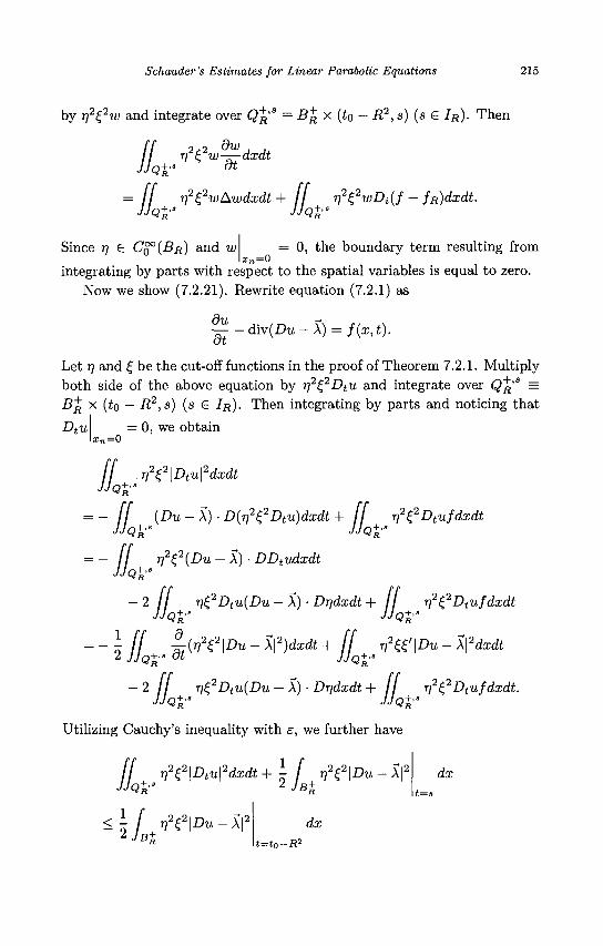
Schauder's Estimates for Linear Parabolic Equations 215
by r72£2w and integrate over Q^'s = B^ x (t0 - R2, s) (s € IR). Then
dw ~dt
[[ rfe^dxdt J Jot-3
'Ql-
if r)2Z2wAwdxdt+ if r)2Z2wDi(f - fR)dxdt. JJQ+-* JJQ+
R'
Since r\ e C^{BR) and w xn=0
= 0, the boundary term resulting from
integrating by parts with respect to the spatial variables is equal to zero. Now we show (7.2.21). Rewrite equation (7.2.1) as
^ - d i v ( £ > u - A ) = / ( M ) .
Let 77 and £ be the cut-off functions in the proof of Theorem 7.2.1. Multiply both side of the above equation by r)2£2Dtu and integrate over Q~^'s = BR x (£0 — R2,s) (s S IR). Then integrating by parts and noticing that
Dtu = 0, we obtain x n =0
II r]2i2\Dtu\2dxdt JJQ+"
: - / / (Du - A) • D{r)2Z2Dtu)dxdt + If rj2Z2Dtufdxdt JJQV JJQRS
- r]2(,2(Du-X)-DDtudxdt JjQf
- 2 / / r)£,2Dtu(Du - A) • Drjdxdt + / / r)2£2Dtufdxdt JjQ+-a JJQ+a
: ~ 2 Hot QR
2
d_
dt (r)2Z2\Du - X\2)dxdt + II iftfl Du - \\2dxdt
II r)Z2Dtu{Du - A) • Drjdxdt + / / r)2£2Dtufdxdt. JJQR-» JJQ+R->
Utilizing Cauchy's inequality with e, we further have
/ / r?Z2\Dtu\2dxdt+\ J 772£2|£>u-A|:
JjQi3 2 JB+ dx
*iL* ?\Du-\\* dx t=t0-R
2
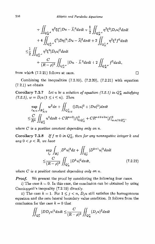
216 Elliptic and Parabolic Equations
+ 11 V2tt'\Du-\\2dxdt+l [[ r)2Z2\Dtu\2dxdt JjQt-s 2 JJQ+,s
+ 4 / / i2\Dr1\2\Du-X\2dxdt + 2 [[ r]2^2f2dxdt
JJQR> JJQ+°
<\ II r,2Z2\Dtu\2dxdt 2 JJQ+--
+ TZ ^r / / \Du - M2dxdt + 2 / / fdxdt, (R - p)2 JJQ+-° JJQ+.>
from which (7.2.21) follows at once. •
Combining the inequalities (7.2.19), (7.2.20), (7.2.21) with equation (7.2.1) we obtain
Corollary 7.2.7 Let u be a solution of equation (7.2.1) in Q^ satisfying (7.2.5), w = Diu(l<i< n): Then
s u p / w2dx+ (\Dtu\2 + \Dw\2)dxdt IRIIJB+,„ ^QR/2
dxdt + CR^2\f\lQl + ^ + 2 + 2 «[ /£ , a / 2 ; Q + ,
V JBj / 2 JJQR/2
<— II u^^^+A.niin+2\t\2 _1_/ .pn+2+2ar/l2
where C is a positive constant depending only on n
Corollary 7.2.8 If f = 0 in Q~^, then for any nonnegative integer k and any 0 < p < R, we have
s u p / \Dku\2dx+ II \Dk+1u\2dxdt h JBi JJQ+
^TB^W llQt}Dku?dxdt' (7-2'22)
where C is a positive constant depending only on n.
Proof. We present the proof by considering the following four cases. i) The case k = 0. In this case, the conclusion can be obtained by using
Caccioppoli's inequality (7.2.19) directly. ii) The case k = 1. For 1 < j < n, DjU still satisfies the homogeneous
equation and the zero lateral boundary value condition. It follows from the conclusion for the case k = 0 that
/ / \DDjU\2dxdt <— ^ / / {Djufdxdt JjQt \ R - P) JJQR
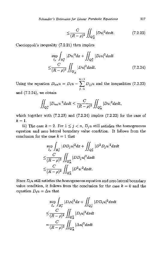
Schauder's Estimates for Linear Parabolic Equations 217
Caccioppoli's inequality (7.2.21) then implies
^wh? L ^ d x i t (T'2-23)
sup / \Du\2dx+ / / \Dtu\2dxdt iP JB+ JJQ+
-whr tfQ+JDu?dxdt <7-2-24)
n - l
Using the equation Dnnu = Dtu — \~] DjjU and the inequalities (7.2.23)
and (7.2.24), we obtain
/ / \Dnnu\2dxdt < — rx / / \Du\2dxdt, JjQt (R ~ P) JJQ+
which together with (7.2.23) and (7.2.24) implies (7.2.22) for the case of k = l.
iii) The case k = 2. For 1 < j < n, DjU still satisfies the homogeneous equation and zero lateral boundary value condition. It follows from the conclusion for the case k = 1 that
sup / \DDju\2dx+ / / \D2Dju\2dxdt iP JB+ JJQ+
C <,n^ „ / / \DDju\2dxdt
(R-P)2JJQ+
c_ •{R-pyjjQ+R
< , „ ^ xo / / \D2u\2dxdt.
Since Dtu still satisfies the homogeneous equation and zero lateral boundary value condition, it follows from the conclusion for the case k = 0 and the equation Dtu = Au that
sup / |D tu\2dx + / / \DDtu\2dxdt Ip JB+ JJQ +
C_ (R-P)2JJQi
C_ \R-P)2JJQ+R
<,„~ ,„ / / \Dtu\2dxdt JJQ+R
/ / \Au\2dxdt JJQt
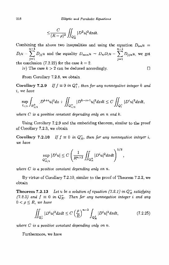
218 Elliptic and Parabolic Equations
\D2u\2dxdt. -{R-PYJIQI
Combining the above two inequalities and using the equation Dnnu = n—1 n - 1
Dtu - 2 J DJJU and the equality Dnnnu = DnDtu — J ^ Djjnu, we get j = i j = i
the conclusion (7.2.22) for the case k = 2. iv) The case A; > 2 can be deduced accordingly. •
Prom Corollary 7.2.8, we obtain
Corollary 7.2.9 If f = 0 in Q~l, then for any nonnegative integer k and i, we have
sup / \Dk+iu\2dx + ff \Dk+i+1u\2dxdt <C ff {D^dxdt, A/a JB+/2 JJQt/2 JJQt
where C is a positive constant depending only on n and k.
Using Corollary 7.2.9 and the embedding theorem, similar to the proof of Corollary 7.2.3, we obtain
Corollary 7.2.10 If f = 0 in Q^, then for any nonnegative integer i, we have
sup |D'u| < C ( - ^ - 2 / / |Z3*«|2dardt
1/2
where C is a positive constant depending only on n.
By virtue of Corollary 7.2.10, similar to the proof of Theorem 7.2.2, we obtain
Theorem 7.2.13 Let u be a solution of equation (7.2.1) in Q^ satisfying (7.2.5) and f = 0 in Q\. Then for any nonnegative integer i and any 0 < p < R, we have
ff ID^dxdt < C (^)n+2 [ ID^dxdt, (7.2.25) JJQt y R / JQ+R
where C is a positive constant depending only on n.
Furthermore, we have
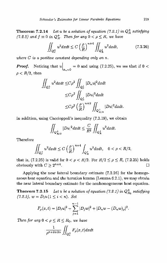
Schauder's Estimates for Linear Parabolic Equations 219
Theorem 7.2.14 Letu be a solution of equation (7.2.1) in Q^ satisfying (7.2.5) and f = 0 in Q\. Then for any 0 < p < R, we have
ff u2dxdt<c(^)n+ ff u2dxdt, (7.2.26)
where C is a positive constant depending only on n.
Proof. Noticing that u = 0 and using (7.2.25), we see that if 0 < x =0
p < R/2, then
/ / u2dxdt <Cp2 / / \Dnu\2dxdt
<Cp2 ff \Du\2dxdt JjQt
<Cp2 (^)n+2 ff \Du\2dxdt.
In addition, using Caccioppoli's inequality (7.2.19), we obtain
/ / \Du\2dxdt < TPT / / u2dxdt. JjQln R JJQt
Therefore
II u2dxdt<c(^Y+ f u2dxdt, 0 < p < R/2, JJQp JQR
that is, (7.2.25) is valid for 0 < p < R/2. For R/2 < p < R, (7.2.25) holds obviously with C > 2n+A. •
Applying the near lateral boundary estimate (7.2.26) for the homogeneous heat equation and the iteration lemma (Lemma 6.2.1), we may obtain the near lateral boundary estimate for the nonhomogeneous heat equation.
Theorem 7.2.15 Let u be a solution of equation (7.2.1) in Q^o satisfying (7.2.5), w = Diu(l <i<n). Set
n - l
Fp(x,t) = \Dtu\2 + Y^ \DJW\2 + \Dnw - (Dnw)p\2.
Then for any 0 < p < R < Ro, we have
p n + 2 + 2a JJ Fp(x,t)dxdt
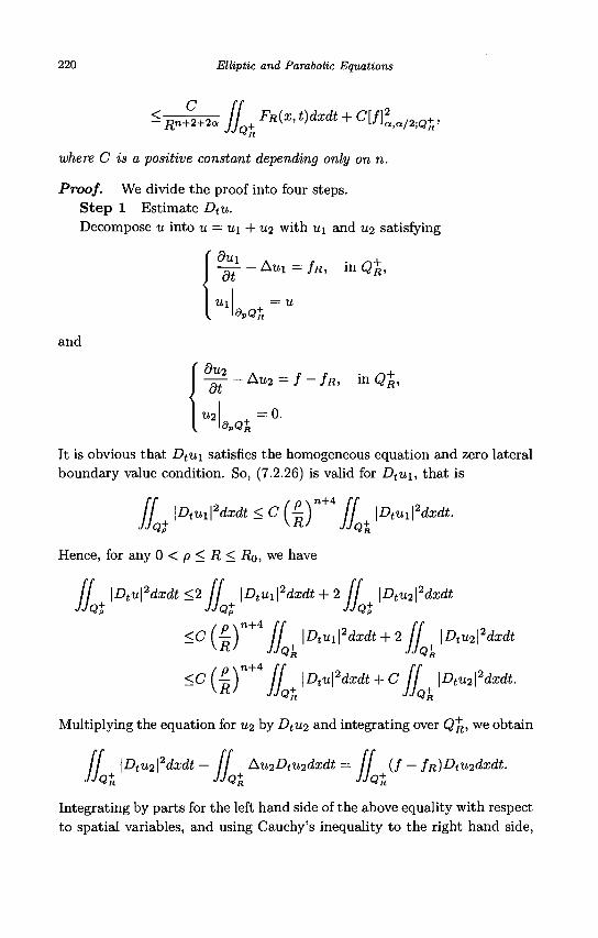
220 Elliptic and Parabolic Equations
<- c If FR(x,t)dxdt + C[f}la/2.Q+R, Rn+2+2oc JJQj
where C is a positive constant depending only on n.
Proof. We divide the proof into four steps. Step 1 Estimate Dtu. Decompose u into u = u\ + u2 with u\ and u2 satisfying
-^r - Aui = fR, in <2£, dt
and
dpQt
- ^ - Au2 = f - fR, in Q-R-,
u2 . = 0 . 9PQ+
R
It is obvious that Dtui satisfies the homogeneous equation and zero lateral boundary value condition. So, (7.2.26) is valid for Dtui, that is
ff \DtUl\2dxdt < C (4)" + / / Wtu^dxdt.
Hence, for any 0 < p < R < RQ, we have
/ / \Dtu\2dxdt<2 \DtUi\2dxdt + 2 \Dtu2\2dxdt
<c(^)n+ ff \Dtu1\2dxdt + 2 ff \Dtu2\
2dxdt V-R / JjQt JJQR
<C(^Y+ ff \Dtu\2dxdt + C ff \Dtu2\2dxdt.
Multiplying the equation for u2 by Dtu2 and integrating over Q^, we obtain
/ / \Dtu2\2dxdt- ff Au2Dtu2dxdt= ff ( / - fR)Dtu2dxdt.
JJQ+ JJQ+ JJQ+
Integrating by parts for the left hand side of the above equality with respect to spatial variables, and using Cauchy's inequality to the right hand side,
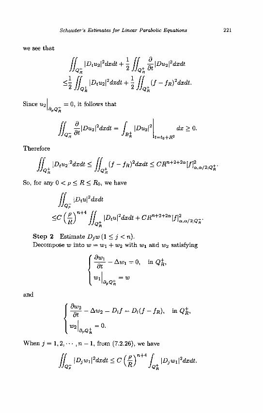
Schauder's Estimates for Linear Parabolic Equations 221
we see that
dxdt
<\ ft \Dtu2\2dxdt+± [[ (f-fR)2dxdt.
1 JJQt l JJQt
Since u2 9pQt = 0, it follows that
dx >0 . t=t0+R2
[[ ^\Du2\2dxdt = I \Du2?
JJQ+ ot JB+
Therefore
ff + \Dtu2\2dxdt < ff (/ - fR)2dxdt < CRn+2+2a[f}2
aa/
So, for any 0 < p < R < Ro, we have
/ / \Dtu\2dxdt JJQt
-c ( l )" + 4 IIQt WtU?dxdt+CRn+2+2aKa/*Qf
Step 2 Estimate DJW(1 < j <n). Decompose w into w = w\ + w2 with w\ and w2 satisfying
' 9wi . „ . „+
— - Aw! = 0, m Q+,
W\ dvQt
and
^--Aw2 = DJ = A ( / - /«), in Q+,
w2 Wt 0.
When j = 1,2, • • • , n - 1, from (7.2.26), we have
/ / |D j U ; i | 2 da ;d t<cf4) n + 4 / \DjWl\2dxdt.
JJQt KKJ JQ+ 'Qt
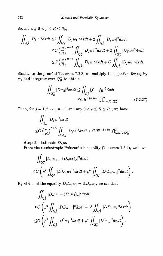
222 Elliptic and Parabolic Equations
So, for any 0 < p < R < RQ,
/ / \Djw\2dxdt<2 \Djw1\2dxdt + 2 \Djw2\
2dxdt JjQi JJQi JJQ+
-C(RT II \DJwi\2(ixdt + 2 (I \DjW2\2dxdt
- C ' ( f l ) n + / / \DM2dxdt + C II \DjW2\2dxdt.
Similar to the proof of Theorem 7.2.3, we multiply the equation for w2 by u>2 and integrate over Q^ to obtain
/ / \Dw2\2dxdt < ft {f-fR)2dxdt
JJQ+ JJQ$
<CRn+2+2«[f}2aa/2.Q+R (7.2.27)
Then, for j = 1,2, • • • , n — 1 and any 0 < p < R < RQ, we have
/ / \Djw\2dxdt
^C ( l ) n + 4 UQ+R \DM2dxdt + CR^2^[f]2aa/2iQ+R
Step 3 Estimate Dnw. From the ^-anisotropic Poincare's inequality (Theorem 1.3.4), we have
/ / \Dnwi - (Dnwi)p\2dxdt
JJQt
<clp2 I \DDnwi\2dxdt + p4 / / \DtDnwi\2dxdt\ .
By virtue of the equality DtDnw\ = ADnw\, we see that
// \Dnwi - (Dnwi)p\2dxdt
JjQt
<C ( p2 If \DDnwi\2dxdt + p* / / |ADnWi\2dxdt)
<C [p2 If \D2Wl\
2dxdt + p4 II \D3Wl\
2dxdt\ .
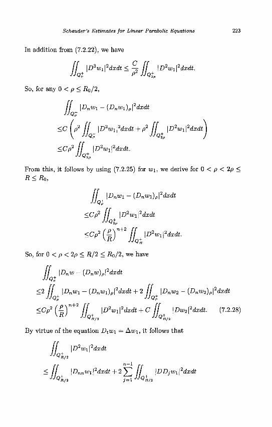
Schauder's Estimates for Linear Parabolic Equations 223
In addition from (7.2.22), we have
/ / ID^^dxdt < -z \\ \D2wi\2dxdt. JjQt P2 JJQt
So, for any 0 < p < R0/2,
// \Dnwi - (Dnwi)p\2dxdt
JJQt
<clp2 ff \D2wi\2dxdt + p2 II \D2wi\2dxdt)
<Cp2 ff \D2Wl\
2dxdt. JJQt
Prom this, it follows by using (7.2.25) for wi, we derive for 0 < p < 1p < R < ilo,
// \Dnw\ - (Dnwi)p\2dxdt
JJQt
<Cp2 ff \D2Wl\
2dxdt JJQt
<Cp2 ( | ) " + 2 [[\D2Wl\
2dxdt.
So, for 0 < p < 2p < R/2 < R0/2, we have
/ / \Dnw - (Dnw)p\2dxdt
JJQt
<2 If \Dnwi - {Dnwi)p\2dxdt + 2 \Dnw2 - {Dnw2)p\
2dxdt JJQt JJQt
<Cp2(£-Y+2 ff \D2wA2dxdt + C ff \Dw2\2dxdt. (7.2.28)
KRJ JJQt,* JJQt/2
By virtue of the equation Dtw\ = Au>i, it follows that
/ / \D2Wl\
2dxdt JJQt„
< ff \Dnnwi\2dxdt + 2y" ff \DDjWi\2dxdt JJQt,* j^i JJQt,2
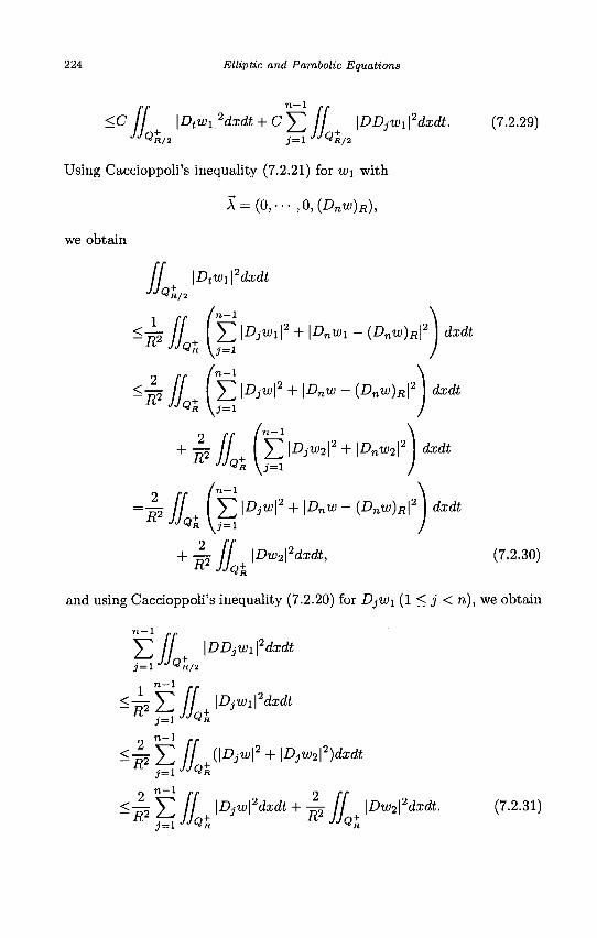
224 Elliptic and Parabolic Equations
<C [[ IDtW^dxdt + cY] if IDDjW^dxdt. (7.2.29) JJQ+R/2 7^1 JJQh2 'R/2 J = l ^R/2
Using Caccioppoli's inequality (7.2.21) for w\ with
X = (0,--- ,0,{Dnw)R),
we obtain
\2dxdt If lA i JJQi/2
^jp Jf +\Y \Diw? + \Dn™ - i.Dnw)R\z I dxdt
+ JJ2 II +[Y \D0W1? + \DnW2? ) dxdt
=IP IJ A Y I ^ I 2 + \ D » W - (D"W)R
and using Caccioppoli's inequality (7.2.20) for DjWi (1 < j < n), we obtain
Ik 2 n~1 rr
-"R2 Y / / +(\Djw\2 + \DjW2\2)dxdt
<4oY If \Djw\2dxdt+-E2 If \Dw2\2dxdt. (7.2.31)
" ~Z[JJQR H JJQt
/n-1
- ^ / / , I Y \DJWl\2 + IA»U>1 - (DnW)R\2 | dxdt
' n - 1
' n - 1
<n-l
dxdt
I H \Dw2\2dxdt, (7.2.30)
R
-- -tR
m o m m l i i - i r ^ 7 O 9 f l \ fi-.r 7 , . ,
n - 1
\DDjWi\2dxdt j = l •'JQR/2
n - 1 ^ Y II , |£j«>il2<*«ft
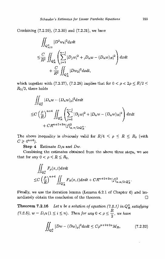
Schauder's Estimates for Linear Parabolic Equations 225
Combining (7.2.29), (7.2.30) and (7.2.31), we have
/ / \D2wi\2dxdt JJQ+
R/2
^§2 If + [Yl \Diwf + \D"W ~ (Dnw)R\2 J dxdt
+ w llQJDw^2dxdt> which together with (7.2.27), (7.2.28) implies that for 0 < p < 2p < R/2 < Ro/2, there holds
/ / \Dnw - (Dnw)p\2dxdt
JjQt
<C ( |)"+4 II+ I 5Z \Diw\2 + \D"W ~ (Dnw)R\2 J dxdt
, f-ipn+2+2alf]2 + L/K VL,a/2;Q+-
The above inequality is obviously valid for R/A < p < R < Ro (with C > 4n+4).
Step 4 Estimate Dtu and Dw. Combining the estimates obtained from the above three steps, we see
that for any 0 < p < R < Ro,
/ / Fp(x,t)dxdt JJQt
~C ( ^ r 4 HQt Ffi(X't)dXdt + CRn+*+2aVt«/2;Qf
Finally, we use the iteration lemma (Lemma 6.2.1 of Chapter 6) and immediately obtain the conclusion of the theorem. •
Theorem 7.2.16 Letu be a solution of equation (7.2.1) in Q^ satisfying
(7.2.5), w = DiU (1 <i <ri). Then for any 0 < p < —, we have
ff \Dw - (Dw)p\2dxdt < Cpn+2+2aMR, (7.2.32)
JJQ+
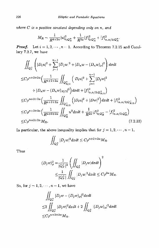
226 Elliptic and Parabolic Equations
where C is a positive constant depending only on n, and
1 • , 2 . 1
Proof. Let i = 1,2,••• ,n — 1. According to Theorem 7.2.15 and Corollary 7.2.7, we have
jj + | \Dtu\2 + Y^ \DJW\2 + \DnW - (Dnw)p\2 J dxdt
+ |D„io - (Dnw)R/2f)dx4t + lf?v/2lQiJ
iCeM2° (s^s JIQi »2 " ' + j ^ l /Ha t + W„/™s)
<C /o"+ 2 + 2 aM f l . (7.2.33)
In particular, the above inequality implies that for j = 1,2, • • • , n — 1,
[[ \DjW\2dxdt < Cpn+2+2aMR. JjQt
Thus
{D><=m\lUDMdxd) Qt\ JjQt -\QJ
So, for j = 1,2, • • • , n — 1, we have
<T-TT / / \Djw\'dxdt < Cp'aMR.
II \DjW — (Djw)p\2dxdt
<2 / / \Djw\2dxdt + 2 / / \{DjW)p\2dxdt
<Cpn+2+2aMR
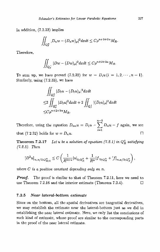
Schauder's Estimates for Linear Parabolic Equations 227
In addition, (7.2.33) implies
/ / \Dnw - (Dnw)p\2dxdt < Cpn+2+2aMR.
JjQt
Therefore,
/ / \Dw - (Dw)p\2dxdt < Cpn+2+2aMR.
JjQt
To sum up, we have proved (7.2.32) for w = Diu(i = 1,2, • • • ,n — 1). Similarly, using (7.2.33), we have
/ / \Dtu - (Dtu)p\2dxdt
JjQt
<2 / / \Dtu\2dxdt + 2 I \(Dtu)p\2dxdt
JjQt JJQt <Cpn+2+2aMR.
7 1 - 1
Therefore, using the equation Dnnu = Dtu — \] D^u — f again, we see i = i
that (7.2.32) holds for w = Dnu. •
Theorem 7.2.17 Let u be a solution of equation (7.2.1) in Q\ satisfying (7.2.5). Then
[£>2<a/2;Q+ /2 < C ( ^ | « | 0 ; Q + + ^ l / l 0 ; Q + + [/]a,a/2 i0+) -
where C is a positive constant depending only on n.
Proof. The proof is similar to that of Theorem 7.2.11, here we need to use Theorem 7.2.16 and the interior estimate (Theorem 7.2.4). •
7.2.5 Near lateral-bottom estimate
Since on the bottom, all the spatial derivatives are tangential derivatives, we may establish the estimate near the lateral-bottom just as we did in establishing the near lateral estimate. Here, we only list the conclusions of such kind of estimate, whose proof are similar to the corresponding parts in the proof of the near lateral estimate.
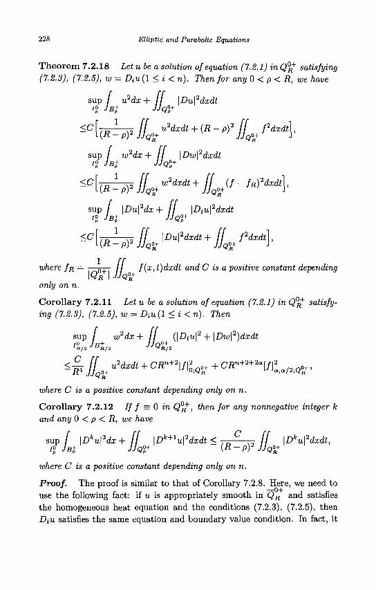
228 Elliptic and Parabolic Equations
Theorem 7.2.18 Letu be a solution of equation (7.2.1) inQR+ satisfying
(7.2.3), (7.2.5), w = Diu(l<i<n). Then for any 0 < p < R, we have
sup / u2dx+ / / \Du\2dxdt i° JB+ JJQ°+
'.mh? IL°+u2dxdt+{R~p? IL - fdxdt <c >Q7
<C dxdt
<C
sup / w2dx + / / \Dw\2dxdt
sup / \Du\2dx+ / / \Dtu\2dxdt i° JB+ JJQ°+
, p l ,2 / / \Du\2dxdt+ [f f2dxdt],
(R - p)2 JJQo+ JJQO+ 1
where / # = -—g — / / f(x, t)dxdt and C is a positive constant depending \QR.\ JJQI+
only on n.
Corollary 7.2.11 Let u be a solution of equation (7.2.1) in Q°R satisfying (7.2.3), (7.2.5), w = Diu(l<i<n). Then
sup / w2dx+ / / (\Dtu\2 + \Dw\2)dxdt
^ f L u 2 d x d t + CRn+2KQ°R+ +CRn+2+2aKa/2-,Q^ JJQR
where C is a positive constant depending only on n.
Corollary 7.2.12 If f = 0 in Q°R , then for any nonnegative integer k and any 0 < p < R, we have
sup / \Dku\2dx + (I \Dk+1u\2dxdt < l J 3 . , II \Dku\2dxdt, 79 JBt JJQ0+ (R-prJjQ0+
where C is a positive constant depending only on n.
Proof. The proof is similar to that of Corollary 7.2.8. Here, we need to use the following fact: if u is appropriately smooth in QR and satisfies the homogeneous heat equation and the conditions (7.2.3), (7.2.5), then Dtu satisfies the same equation and boundary value condition. In fact, it
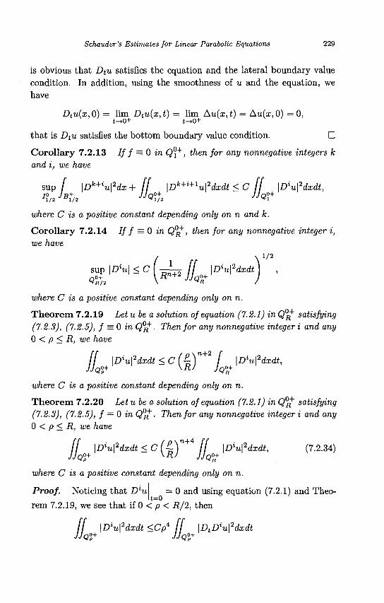
Schauder's Estimates for Linear Parabolic Equations 229
is obvious that Dtu satisfies the equation and the lateral boundary value condition. In addition, using the smoothness of u and the equation, we have
Dtu(x,0) = lim Dtu(x,t) = lim Au(x,t) = Au(x, 0) = 0, t->0+ t->0+
that is Dtu satisfies the bottom boundary value condition. •
Corollary 7.2.13 If f = 0 in Q?+ , then for any nonnegative integers k and i, we have
sup / \Dk+iu\2dx + [[ \Dk+i+1u\2dxdt < C [[ [D^dxdt,
where C is a positive constant depending only on n and k.
Corollary 7.2.14 If f = 0 in Q°R , then for any nonnegative integer i, we have
I \ 1/2
sup | ^ | <C \*JJ" JD^dxdA ,
where C is a positive constant depending only on n.
Theorem 7.2.19 Letu be a solution of equation (7.2.1) inQ°^~ satisfying (7.2.3), (7.2.5), f = 0 in Q°R~• Then for any nonnegative integer i and any 0 < p < R, we have
[[ {D'uPdxdt < C (£-Y+ f iD^dxdt, JJQ°+ \R/ JQ°+
where C is a positive constant depending only on n.
Theorem 7.2.20 Let u be a solution of equation (7.2.1) in Q^+ satisfying (7.2.3), (7.2.5), f = 0 in Q0^ • Then for any nonnegative integer i and any 0 < p < R, we have
If {D^dxdt < C ( " | ) " + ft ^ufdxdt, (7.2.34)
where C is a positive constant depending only on n.
Proof. Noticing that D%u = 0 and using equation (7.2.1) and Theo
rem 7.2.19, we see that if 0 < p < R/2, then
ff ID^dxdt <Cp4 [[ WtD^dxdt JJQ°P
+ JJQ°+
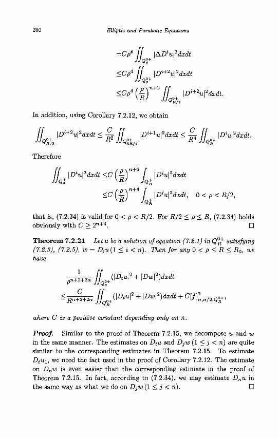
230 Elliptic and Parabolic Equations
=CpA (I lADVdaaft JJQV-
<CpA II \Di+2u\2dxdt JJQI+
<CpA f 4 ) " + 2 / / \Di+2u\2dxdt. KRJ JJQV,*
In addition, using Corollary 7.2.12, we obtain
/ / \Di+2u\2dxdt <%r II \Di+1u\2dxdt < £ II l&ufdxdt. JJQV/2 R 2JJQI+/4
R4JJQ°R+
Therefore
II {D^dxdt^cl^-Y^ I ID^dxdt J Jot yRj
JQ+
<c(^)n+ I {D^dxdt, 0<p<R/2, y R / JQ+
R
that is, (7.2.34) is valid for 0 < p < R/2. For R/2 < p < R, (7.2.34) holds obviously with C > 2n + 4 . •
Theorem 7.2.21 Letu be a solution of equation (7.2.1) inCf^ satisfying (7.2.3), (7.2.5), w = Dtu (1 < i < n). Then for any 0 < p < R < R0, we have
^nJ^ /L^i2+M)***+^[/]^/2iQoR+, JJQR
where C is a positive constant depending only on n.
Proof. Similar to the proof of Theorem 7.2.15, we decompose u and w in the same manner. The estimates on DfU and DjW (1 < j < n) are quite similar to the corresponding estimates in Theorem 7.2.15. To estimate Dtu\, we need the fact used in the proof of Corollary 7.2.12. The estimate on Dnw is even easier than the corresponding estimate in the proof of Theorem 7.2.15. In fact, according to (7.2.34), we may estimate Dnu in the same way as what we do on DjW (1 < j < n). •
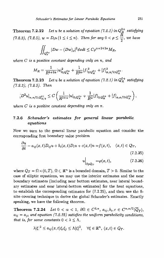
Schauder 's Estimates for Linear Parabolic Equations 231
Theorem 7.2.22 Let u be a solution of equation (7.2.1) in Q0^ satisfying
(7.2.3), (7.2.5), w = Dtu (1 < i < n). Then for any 0 < p<—, we have
[[ \Dw - (Dw)p\2dxdt < Cpn+2+2aMR,
JJQ°P+
where C is a positive constant depending only on n, and
MR = ^4+2^lUlo;Q°R+ + ;R2^lo;Q0R+ + ^l,a/2;Q°R
+-
Theorem 7.2.23 Let u be a solution of equation (7.2.1) in Q°R+ satisfying
(7.2.3), (7.2.5). Then
lD2u]a,a/2;Q°+/2 < C ( ] ^ M o ; Q R + + Jp\f\o;Q°+ + [/]a,a/2;Q°+J ,
where C is a positive constant depending only on n.
7.2.6 Schauder's estimates for general linear parabolic equations
Now we turn to the general linear parabolic equation and consider the corresponding first boundary value problem
dii
— - aij(x,t)Diju + bi(x,t)DiU + c(x,t)u =f(x,t), (x,t) € QT,
(7.2.35)
u =tfi(x,t), (7.2.36) dpQr
where QT = O x (0, T), Q c M™ is a bounded domain, T > 0. Similar to the case of elliptic equations, we may use the interior estimates and the near boundary estimates (including near bottom estimates, near lateral boundary estimates and near lateral-bottom estimates) for the heat equations, to establish the corresponding estimates for (7.2.35), and then use the finite covering technique to derive the global Schauder's estimates. Exactly speaking, we have the following theorem. Theorem 7.2.24 Let 0 < a < 1, dfl 6 C2'a, aihbuc £ Ca>a/2(QT), aij = aji and equation (7.2.35) satisfies the uniform parabolicity conditions, that is, for some constants 0 < A < A,
A|e|2 < a«(a,t)&& < A|£|2, V£ € R", (x,t) € QT-
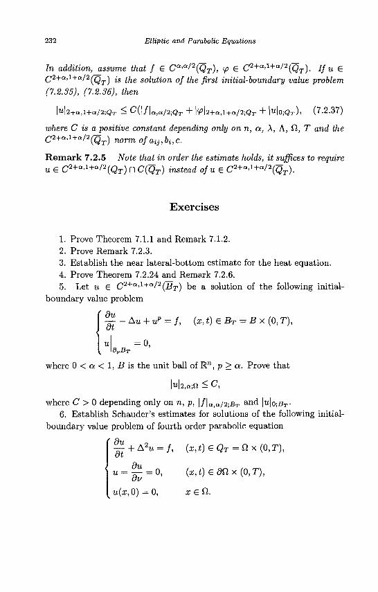
232 Elliptic and Parabolic Equations
In addition, assume that f £ Ca'a/2(QT), <p £ C 2 + a > 1 + a / 2 (Q T ) . If u £ C2+a'1+a/2(QT) is the solution of the first initial-boundary value problem (7.2.35), (7.2.36), then
M2+a, l+<*/2;Q T ^ C{\f\a,a/2;QT + \p\2+a,l+a/2;QT + \u\o-,QT)> (7 .2 .37)
where C is a positive constant depending only on n, a, A, A, f2, T and the C2+a,l+a/2(QT) norm 0f a^^ c,
Remark 7.2.5 Note that in order the estimate holds, it suffices to require u £ C2+a>l+a'2{QT) n C(QT) instead ofu£ C2+a'1+a'2(JQT).
Exercises
1. Prove Theorem 7.1.1 and Remark 7.1.2. 2. Prove Remark 7.2.3. 3. Establish the near lateral-bottom estimate for the heat equation. 4. Prove Theorem 7.2.24 and Remark 7.2.6. 5. Let u £ C2+a>1+a/2{BT) be a solution of the following initial-
boundary value problem
~^-Au + up = f, (x,t)£BT = Bx(0,T),
dpBT
0,
where 0 < a < 1, B is the unit ball of W1, p > a. Prove that
where C > 0 depending only on n, p, |/ |Q,a/2 ;BT and |U|O;BT-
6. Establish Schauder's estimates for solutions of the following initial-boundary value problem of fourth order parabolic equation
f du dt
+ A2u = f, (x,t)£QT = Clx(0,T),
du u = — = 0,
ov
u(x,Q) = 0 ,
(x,t)£dQ,x (0,T),
x £ £1.
Chapter 8
Existence of Classical Solutions for Linear Equations
In this chapter, we establish the existence theory of classical solutions for linear elliptic and parabolic equations of second order.
8.1 Maximum Principle and Comparison Principle
The existence of classical solutions is based on Schauder's estimates. In addition, the L00 norm estimate on solutions is also needed. In this section, we introduce the maximum principle, which will be used to establish the L°° norm estimate and comparison principle on classical solutions.
8.1.1 The case of elliptic equations
Consider the following linear elliptic equation
Lu=—aij(x)DijU + bi(x)DiU + c(x)u = f(x), x £ fi, (8.1.1)
where Q, C W1 is a bounded domain, a^ = dji and for some constant A > 0,
aij(x)^j > A|£|2, V f e R " , i e ( l .
Theorem 8.1.1 (Maximum Principle) Let c(x) > 0, bi(x) and c(x) be bounded inQ., u G C2(f2) n C(H) satisfy Lu = f < 0 (> 0) in Q.. Then
sup u(x) < sup u+ (x) (inf u(x) > inf u_ (x)), n an \ n an J
where u+ = max{it,0}, u_ = min{w,0}.
233
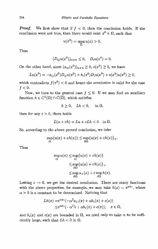
234 Elliptic and Parabolic Equations
Proof. We first show that if / < 0, then the conclusion holds. If the conclusion were not true, then there would exist x° € Cl, such that
u(x°) = rnaxu(x) > 0. n
Thus
(DijU(x°))nxn < 0, DiU(x°) = 0.
On the other hand, since (aij(x°))nxn > 0, c(x°) > 0, we have
Lu(x°) = -aij{x0)Diju{x0) + bi(x0)Diu{x0) + c(x°)u(x°) > 0,
which contradicts f(x°) < 0 and hence the conclusion is valid for the case / < 0 .
Now, we turn to the general case / < 0. If we may find an auxiliary function h G C2(Q) fl C(Q), which satisfies
h > 0, Lh<0, in fi,
then for any e > 0, there holds
L(u + eh) = Lu + eLh < 0 in 9,.
So, according to the above proved conclusion, we infer
sup{'u(a;) + eh(x)} < sup{u(x) + eh(x)}+. n an
Thus
supu(a;) <sup{u(x) +eh(x)} n n
< sup{w(x) + eh(x)}+ an
< sup u+ (x) + e sup h{x). an an
Letting e —> 0, we get the desired conclusion. There are many functions with the above properties, for example, we may take h{x) = e a x i , where a > 0 is a constant to be determined. Noticing that
Lh{x) =eaxi(-a2an(x) + ah(x) + c(x))
<e Q X l ( -a 2 A + a6i(a;) + c(x)), x £ ft,
and bi(x) and c(x) are bounded in fi, we need only to take a to be sufficiently large, such that Lh < 0 in Cl.
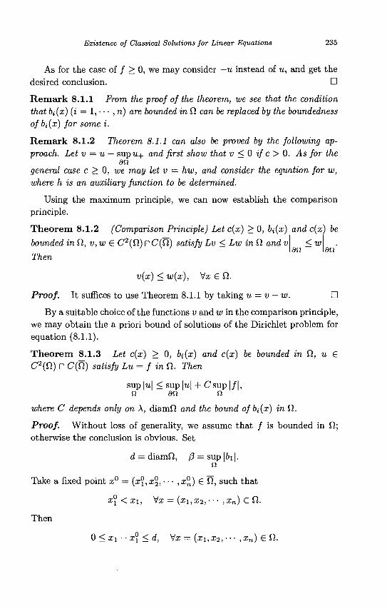
Existence of Classical Solutions for Linear Equations 235
As for the case of / > 0, we may consider — u instead of u, and get the desired conclusion. •
Remark 8.1.1 From the proof of the theorem, we see that the condition that bi(x) (i = 1, • • • ,n) are bounded in fi can be replaced by the boundedness ofbi(x) for some i.
Remark 8.1.2 Theorem 8.1.1 can also be proved by the following approach. Let v = u — supu+ and first show that v < 0 if c > 0. As for the
an general case c > 0, we may let v = hw, and consider the equation for w, where h is an auxiliary function to be determined.
Using the maximum principle, we can now establish the comparison principle.
Theorem 8.1.2 (Comparison Principle) Let c(x) > 0, bi(x) and c{x) be
bounded in Vt, v,w € C2(f2) l~lC(f2) satisfy Lv < Lw in Cl and v
Then
< w an an
v(x) < w(x), \tx £ Q,.
Proof. It suffices to use Theorem 8.1.1 by taking u = v — w. •
By a suitable choice of the functions v and w in the comparison principle, we may obtain the a priori bound of solutions of the Dirichlet problem for equation (8.1.1).
Theorem 8.1.3 Let c(x) > 0, bi(x) and c(x) be bounded in Q, u € C2(Cl) H C(fi) satisfy Lu = f in Q. Then
sup|w| < sup|u| + C sup | / | , Q an n
where C depends only on \, diamfi and the bound ofbi(x) in Q.
Proof. Without loss of generality, we assume that / is bounded in 0; otherwise the conclusion is obvious. Set
d = diamfi, /3 = sup |6i|. a
Take a fixed point x° = (x°,x®,- • • ,a;°) € fi, such that
x\ < xi, Va; = {xi,x%, • • • ,xn) e fl.
Then
0 < Xi — i j < d, Vx = (xi,X2,--• ,xn) €0,.
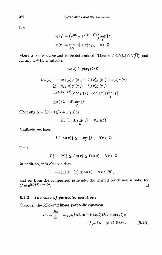
236 Elliptic and Parabolic Equations
Let
<?(*!) = ( e Q d - e ^ - * ? > ) sup | / | ,
w(x) =sup |u | +g(xi), x € f2, an
where a > 0 is a constant to be determined. Then w e C2(f2) n C(D.), and for any x £ il, w satisfies
w(x) > g(xi) > 0,
Lw(x) = - an(x)g"(xi) + bi{x)g'{x{) + c{x)w{x)
> - an(x)g"(xi) + bi(x)g'(xi)
=ea^-x°\a2an(x) - ah(x)) sup | / | n
> a ( a A - / 3 ) s u p | / | .
Choosing a = (j3 + 1)/A + 1 yields
Lw(x) > sup | / | , Mx £ Q. n
Similarly, we have
L{-w(x)} < - sup | / | , Vx £ CI.
Thus
L{-w{x)} < Lu(x) < Lw(x), Mx £ ft.
In addition, it is obvious that
—w{x) < u(x) < w(x), Vx £ dfl,
and so, from the comparison principle, the desired conclusion is valid for
c = e((/3+i)/A+i)d_ •
8.1.2 The case of parabolic equations
Consider the following linear parabolic equation
Ou Lu=— aij(x,t)DijU + bi(x,t)DiU + c(x,t)u
= f(x,t), {x,i)£QT, (8.1.2)
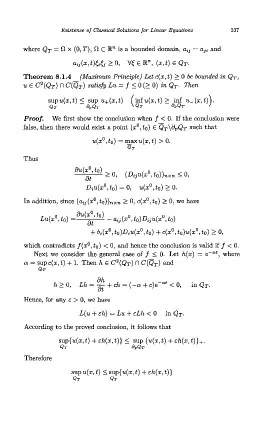
Existence of Classical Solutions for Linear Equations 237
where QT = fi x (0,T), f2 C Rn is a bounded domain, ay = a,ji and
Oij(x, t)tej > 0, V£ E Rn, (x, t) € QT.
Theorem 8.1.4 (Maximum Principle) Let c(x, t) > 0 be bounded in QT, u e C2{QT) n C(QT) satisfy Lu = f < 0 (> 0) inQT- Then
supu(a;,t) < sup n + (x , t ) ( infu(x,t) > inf u-(x,t)\. QT dpQT ^QT BVQT '
Proof. We first show the conclusion when / < 0. If the conclusion were false, then there would exist a point (x°,to) S QT\9PQT such that
u(x°, to) = max u(x, t) > 0. QT
Thus
A M ( J ; 0 , to) = 0, u(x°, t0) > 0.
In addition, since {aij(x°,to))nxn > 0, c(x°,to) > 0, we have
Lu(x°,t0) = - - ^ aij(x° ,t0)Diju(x0 , t0)
+ 64(x°, t 0 ) A « ( i ° , t0) + c(x°, t0)u(x°, t0) > 0,
which contradicts f(x°, to) < 0, and hence the conclusion is valid if / < 0. Next we consider the general case of / < 0. Let h(x) = e~at, where
a = supc(x.t) + 1. Then h £ C2(QT) n C(QT) and QT
h>0, Lh = — + ch = (-a + c)e~at < 0, in QT-at
Hence, for any e > 0, we have
L(u + eh) = Lu + eLh < 0 in QT-
According to the proved conclusion, it follows that
Therefore
sup{u(a;) t) + eh(x, t)} < sup {u(x, t) + eh(x, t)}+. QT dpQT
sup u(x, t) < sup{w(a;, t) + eh(x, t)} QT QT
238 Elliptic and Parabolic Equations
< sup {u(x,t) + eh(x,t)}+ dpQT
< sup u+(x,t) + e sup h(x,t). dpQx dpQr
Letting e —» 0, we get the desired conclusion. For the case of / > 0, we need only to consider — u instead of u. •
Remark 8.1.3 In Theorem 8.1.2, we merely assume the parabolicity condition rather than the uniform parabolicity condition for equation (8.1.2), and no boundedness condition for bi is assumed.
If we do not assume the condition c(x, t) > 0, then the above maximum principle is invalid. However, we still have the following useful result.
Theorem 8.1.5 Let c(x,t) be bounded in QT, U G C2(QT) n C(QT) satisfy Lu = f < 0 in QT and sup u(x,t) < 0. Then
9PQT
sup u(x,t) < 0. QT
Proof. Let CQ = inf c(x,t) and set QT
v(x,t) =ecotu(x,t).
Then v satisfies
— - aij(x,t)Dijv + bi(x,t)DiV + {c(x,t) - CQ)V = eCotf(x,t) < 0,
(x,t)eQT.
Noticing that c(x,t) — CQ > 0 in QT, from Theorem 8.1.4, we obtain
supv(x,t) < sup v+(x,t) = sup eCotu+(x,t) = 0 , QT 9PQT 9PQT
which leads to the conclusion of the theorem. •
Applying Theorem 8.1.5, we may establish the following comparison principle.
Theorem 8.1.6 (Comparison Principle) Assume that c(x,t) is bounded
in QT, v,w £ C2(QT) n C(QT) satisfy Lv < Lw in QT and v < 9PQT
w . Then dpQT
v(x,t) <w(x,t), V(x,t)€QT-
Existence of Classical Solutions for Linear Equations 239
Proof. We may take u = v — w in Theorem 8.1.5 to obtain the desired conclusion. •
Similar to the case of elliptic equations, by suitably choosing the functions v and w in the comparison principle, we may obtain the a priori bound for solutions of the first initial-boundary value problem for equation (8.1.2).
Theorem 8.1.7 Let c(x,t) > 0 and be bounded in QT, U G C2(QT) l~l C(QT) satisfy Lu = f in QT- Then
s u p | u | < sup |u| + T s u p | / | . QT dpQT QT
Proof. Without loss of generality, we assume that / is bounded in QT; otherwise the conclusion is obvious. Let
w(x,t) = sup |u |-Msup | / | , (x,t) G QT-9PQT QT
Then w G C2(QT) l~l C(QT) and for any (x, t) G QT, we have
Lw(x,t) = sup | / | + c(x, t)w(x, t) > sup | / | . QT QT
Similarly, for any (x,t) G QT, we also have
L{-w(x,t)} < - s u p | / | . n
Thus
L{-w(x,t)} < Lu(x,t) < Lw{x,t), V(x,t) G QT-
In addition, it is obvious that
—w(x, t) < u(x,t) < w{x,t), V(x,t) G 8PQT,
from which and the comparison principle we get the desired conclusion. •
Theorem 8.1.8 Let c(x,t) be bounded in QT, CQ = min{0,inf c(x,t)}, QT
u G C2(QT) n C(QT) satisfy Lu = f inQT- Then
sup|u| < e~coT [ sup | u | + T s u p | / | 1 . QT \dpQT QT J
240 Elliptic and Parabolic Equations
Proof. Let
v{x,t) = eCotu(x,t), (x,t) € QT.
Then v satisfies
dv
— - aij(x,t)Dijv + bi(x,t)DiV + (c(x,t) - CQ)V = eCotf{x,t),
{x,t)£QT.
Noticing that c(x, t) - CQ > 0 in QT, from Theorem 8.1.7, we have sup|u| < sup \v\ +Tsup | e C o t / | , QT &VQT QT
that is
sup|eC o tu|< sup |eC o*u|+Tsup|eC o t / | -QT 9PQT QT
It follows from Co < 0 that
s u p | u | < e C°T I sup | u | + T s u p | / | QT \9PQT QT
D
8.2 Existence and Uniqueness of Classical Solutions for Linear Elliptic Equations
In this section, we first investigate the existence of C2'a(fl) solutions and C2,a(fl) n C(fi) solutions for Poisson's equation and then investigate the existence of the same kinds of solutions for general linear elliptic equations.
8.2.1 Existence and uniqueness of the classical solution for Poisson's equation
Consider the Dirichlet problem for Poisson's equation
-Au = / , i £ f l , (8.2.1)
a n =<,, (8.2.2)
where (1 C 1 " is a bounded domain. We first prove the existence and uniqueness of its C2,a(Q) solution.
Existence of Classical Solutions for Linear Equations 241
Theorem 8.2.1 Let dQ £ C°°, 0 < a < 1, / e Ca(£2), <p G C2'a(Q). Then problem (8.2.1), (8.2.2) admits a unique solution u £ C2'a(Q,).
Proof. Without loss of generality, we assume that <p = 0. Otherwise, we may consider the equation for w = u—<p. Using the standard approximation technique, we may choose a function fe € C°°(0), such that
|/e|a;fJ < 2 | / | Q ; n
and fs converges to / uniformly on Q. as e —> 0. Consider the approximate problem
-Au = fe(x), xeCl,
u\ = 0 . Ian
By the I? theory (Theorem 2.2.5 of Chapter 2), we see that the above problem admits a unique solution ue € C°°(fi). Prom the global Schauder's estimate (Theorem 6.3.1 of Chapter 6), we have
|«e|2,a;fi < C ( | / e | a ; n + |ue |o ;n)-
Using the maximum principle (Theorem 8.1.3) yields
k l o ; n < C|/e |0 in < C | / e | a . n < C | / | a . n .
Thus
\u£\2,a-n < C | / | a ; n.
The constant C in the above formula is independent of e. By Arzela-Ascoli's theorem, there exists a subsequence of {u£}, denoted by itself, and a function u € C2'a(Q,), such that
ue—*u, Due^>Du, D2uE^>D2u
uniformly on fi as e —> 0. Letting e —> 0 in the approximate problem, we see that u satisfies equation (8.2.1) and the boundary value condition
u = 0 . So, we have proved the existence of solutions. The uniqueness an
follows from the maximum principle. •
In Theorem 8.2.1, it is assumed that the domain fi has C°° smooth boundary, which means that the theorem could not be applied even to Poisson's equation in square domain. In what follows, we will relax the
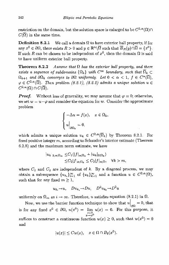
242 Elliptic and Parabolic Equations
restriction on the domain, but the solution space is enlarged to be C2'a(D.)n C(Q) in the same time.
Definition 8.2.1 We call a domain 0 to have exterior ball property, if for any x° € dQ, there exists R > 0 and y e R n \ f i such that ~BR(y)C\Ti = {a;0}. If such R can be chosen to be independent of x°, then the domain Q is said to have uniform exterior ball property.
Theorem 8.2.2 Assume that Cl has the exterior ball property, and there exists a sequence of subdomains {Clk} with C°° boundary, such that £lk c flfc+i and dClk converges to d£l uniformly. Let 0 < a < 1, f £ Ca(fi), (p € C2 , a(fi). Then problem (8.2.1), (8.2.2) admits a unique solution u € C2'Q(fi)nC(n).
Proof. Without loss of generality, we may assume that tp = 0; otherwise, we set w = u—(p and consider the equation for w. Consider the approximate problem
Au = /(a:), x € fife,
= 0,
which admits a unique solution Uk G C2'a(Qk) by Theorem 8.2.1. For fixed positive integer m, according to Schauder's interior estimate (Theorem 6.2.8) and the maximum norm estimate, we have
|Wfc|2,a;fim <Cl{\f\a-Qk + |Mk|o;fifc)
<C2 | / |a ;n f e < Cal/Ujn, Vfc > m,
where C\ and C-x are independent of k. By a diagonal process, we may obtain a subsequence { u ^ } ? ^ of {u^^Li and a function u € C2,a(f2), such that for any fixed m > 1,
uki-*u, Duki-+Du, D2uki-^D2u
uniformly on Qm as i —> oo. Therefore, u satisfies equation (8.2.1) in fi.
Now, we use the barrier function technique to show that u = 0 , that dn
is for any fixed a;0 £ dD., u(x°) = lim u(x) = 0. For this purpose, it • El !
X—>X°
suffices to construct a continuous function w(x) > 0, such that w(x°) = 0 and
|u(aj)| < Cto(a;), a; £ fin Bs(x°).
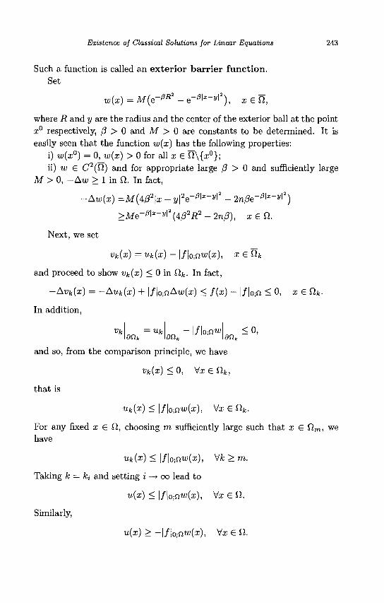
Existence of Classical Solutions for Linear Equations 243
Such a function is called an exterior barrier function. Set
c?2 _ f l l „ . | 2 \ W (x) = M(e-f}R -*-P\*-v\'), i d ,
where R and y are the radius and the center of the exterior ball at the point x° respectively, /3 > 0 and M > 0 are constants to be determined. It is easily seen that the function w(x) has the following properties:
i) w(x°) = 0, w{x) > 0 for all x G Ti\{x0}; ii) w G C2(Q) and for appropriate large /3 > 0 and sufficiently large
M > 0, -Aw > 1 in fi. In fact,
-Aw(x) =M(Ap2\x - yfe-®x-y\2 - 2n(3e-^x-y]?)
>Me-Wx-yf{4p2R2 - 2np), x G n .
Next, we set
vk{x) = uk(x) - \f\o-,nw(x), x G Qfc
and proceed to show Vk(x) < 0 in f2fc. In fact,
-Awfc(x) = -Auk(x) + \f\0-nAw(x) < f(x) - | / |0 ;n < 0, i G fifc.
In addition,
Vfc dak
Uk an,
- \f\o-,nw dak
<0 ,
and so, from the comparison principle, we have
Vk{x) < o, \fx e Ofc,
that is
uk{x) < \f\o-nw{x), Vx G fife.
For any fixed x G fi, choosing m sufficiently large such that a; G flm, we have
«k(aO < \f\o-,nw(x), Vfc > m.
Taking k = hi and setting i —* oo lead to
w(z) < |/|o;nty(ar), Vx G ft.
Similarly,
u(#) > -\f\o-,nw(x), \/x G ft.
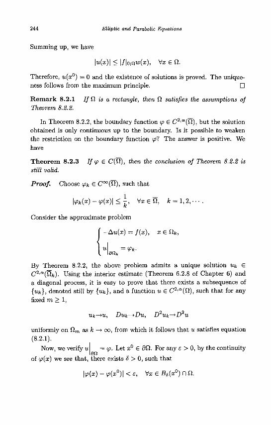
244 Elliptic and Parabolic Equations
Summing up, we have
\u(x)\ < \f\o-,UW(x), Vx G ft.
Therefore, u(x°) — 0 and the existence of solutions is proved. The uniqueness follows from the maximum principle. •
Remark 8.2.1 If 0. is a rectangle, then 0, satisfies the assumptions of Theorem 8.2.2.
In Theorem 8.2.2, the boundary function ip G C2,a(Cl), but the solution obtained is only continuous up to the boundary. Is it possible to weaken the restriction on the boundary function </?? The answer is positive. We have
Theorem 8.2.3 If tp G C(fi), then the conclusion of Theorem 8.2.2 is still valid.
Proof. Choose tpk G C°°(fi), such that
\<Pk(x) - <p(x)\ < - , VxGft, fc = l , 2 , - - - .
Consider the approximate problem
-Au(x) = f(x), x G Clk,
By Theorem 8.2.2, the above problem admits a unique solution Uk G C2'a(fifc). Using the interior estimate (Theorem 6.2.8 of Chapter 6) and a diagonal process, it is easy to prove that there exists a subsequence of {uk}, denoted still by {wfc}, and a function u € C2,Q(fi), such that for any fixed m > 1,
Uk—*u, Duk—^Du, D Uk—>D u
uniformly on Om as k —» oo, from which it follows that u satisfies equation (8.2.1).
Now, we verify u = <p. Let a;0 G 9fi. For any e > 0, by the continuity an
of ip(x) we see that, there exists 5 > 0, such that
\<p(x) - <p(x°)\ < e, Vx G B,5(x0) n ft.
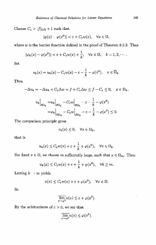
Existence of Classical Solutions for Linear Equations 245
Choose Ce > |/|o;fi + 1 such that
\ip(x)-tp(x0)\<e + Csw(x), Vxeil,
where w is the barrier function defined in the proof of Theorem 8.2.2. Thus
Set
Then
\<pk{x) - <p(x°)\ < e + Cew(x) +-, Vx£il, A; = 1,2,
vk(x) = uk(x) - Cew(x) - £ - T - tp(x°), x € ilk-It
-Avk = -Auk + CEAw = f + CeAw < f - C£ < 0, x e ilk,
1 Vk
dilk
=Uk
=<Pk
an i
an*
-a™
• C e w
ant A;
- £ - - - <f(x°) < 0.
The comparison principle gives
Vk{x) < 0, Vx G fifc,
that is
Ufc(z) < C £ w;(x)+e+ - +<p(x°), Vx £ ilk-
For fixed i S ft, we choose m sufficiently large, such that x £ ilm. Then
uk(x) < Cew(x)+e + - +<p(x°), Vk > m. k
Letting k —> oo yields
u(x) < Ceiv(x)+e + <p(x°), Vx£il.
So
lim u(x) < e + ip(x°). X—>X°
By the arbitrariness of e > 0, we see that
lim u{x) < (p(x ) .
246 Elliptic and Parabolic Equations
Similarly, we obtain
Summing up, we have
lim u(x) > ip(x°). x—>x°
lim u(x) = <p{x°). x—>x°
Thus the existence is proved. The uniqueness of solutions follows from the maximum principle. •
8.2.2 The method of continuity
Contraction Mapping Principle Let T be a contraction mapping on the Banach space B, that is, there exists 0 < 6 < 1, such that
\\Tu-Tv\\<9\\u-v\\, Mu,v£B. (8.2.3)
Then T admits a unique fixed point, that is, the operator equation
Tu = u
admits a unique solution u € B.
Proof. For fixed UQ £ B, set
Ui = Tui-i, i = 1,2, ••• .
For any positive integer 1 < i < j , using (8.2.3), we obtain
3
| |U j -U t | | < ^J \\uk -Ufc-l| | k=i+l
3
= ^2 WTuk-l ~Tuk-2\\ k=i+l
< J2 0*-1||ui-«o|| k=i+l
ai
<^—^Iki — "oil -*0 (i->oo).
Existence of Classical Solutions for Linear Equations 247
So, {ui} is a Cauchy sequence, and from the completeness of B, it converges to some u € B. Prom (8.2.3) we see that T is continuous, and so
Tu = lim Tm = lim Uj+i = u. i—>oo i—>oo
The uniqueness follows directly from (8.2.3). •
Remark 8.2.2 From the proof of the theorem, we see that the conclusion is still valid if we replace B by any closed subset of B.
The Method of Continuity Let B be a Banach space, V be a normed linear space, TQ and Ti be bounded linear operators from B to V. Set
TT = (1-T)TO + TTU r e [0,1].
/ / there exists some constant C > 0, such that
\\u\\B < C\\TTu\\v, UGB,T€[0, 1], (8.2.4)
then Ti maps B onto V if and only if To maps B onto V.
Proof. Let s € [0,1] and Ts maps B onto V. By (8.2.4), we see that Ts is injective and so the inverse map T " 1 : V —> B exists. For T £ [ 0 , l ] , « £ y , the operator equation TTu = v is equivalent to the equation
Tsu = v + (Ts - TT)u = v + (T - s)(T0 - Ti)u.
Furthermore, since T~x exists, it is also equivalent to
u = T~lv + (T - s)T-\T0 - 2\)u = Tu.
If
| T _ s | < ( 5 s C ( | | T o | | + ||T1|| + 1) '
then from (8.2.4), we see that T : B —> B is a contraction map. According to the contraction mapping principle, for any s £ [0,1] satisfying \T — s\ < 8, the map TT is bijective. We decompose [0,1] into several intervals with their length less than 5. It is easy to see that if for some fixed To € [0,1] (in particular for ro = 0 or ro = 1), TT0 is bijective, then for all r € [0,1], TT is bijective too. •
Remark 8.2.3 The method of continuity shows that the invertibility of a bounded linear operator can be deduced from the invertibility of another similar kind of operators.
248 Elliptic and Parabolic Equations
8.2.3 Existence and uniqueness of classical solutions for general linear elliptic equations
By the method of continuity, we may extend the above results about the Dirichlet problem (8.2.1), (8.2.2) for Poisson's equation to the Dirichlet problem for general linear elliptic equation
—aij(x)DijU + bi(x)DiU + c(x)u =f{x), x e f2, (8.2.5)
en =*> ^
where fl C 1 " is a bounded domain, aij,bi,c £ Ca(Q,), c > 0, ai7- = a^, and there exists some constants 0 < A < A, such that
A|£|2 < o^aO&fc < A|£|2, V£ £ l " , i e fl. (8.2.7)
Theorem 8.2.4 Let dtt e C°°, 0 < a < 1, 0^,^,0, f € Ca(U), c > 0, ip € C 2 ' a (0) , ay = a-ji satisfy (8.2.7). Then problem (8.2.5), (8.2.6) admits a unique solution u e C2'a(Q).
Proof. Without loss of generality, we may assume that tp = 0. Otherwise, we consider the equation for w = u — <p.
Let
LQU = — Au,
L\u = — aij(x)DijU + bi(x)DiU + c{x)u.
Consider the family of elliptic equations with a parameter r ,
LTU = {1-T)L0U + TL1U = f, 0 < r < l , (8.2.8)
where the coefficients of second order term satisfy (8.2.7) with A, A taken as
Ar = min{l, A}, A r = max{l, A}.
LT can be regarded as a linear operator from the Banach space B = {u e C2'a(Q) : u\dn = 0} to the normed linear space V = Ca(Ti). So the solvability of problem (8.2.8), (8.2.6) is equivalent to the invertibility of the operator LT. Let u € B be a solution of problem (8.2.8), (8.2.6). According to Schauder's estimates (Theorem 6.3.1 of Chapter 6) and the maximum norm estimates (Theorem 8.1.3), and noticing the assumption (p = 0, we have
|u|2,a;n < Cf l /Ujn + Mo;fi) < C | / | a i n , T G [0, 1],
Existence of Classical Solutions for Linear Equations 249
that is
\\u\\B<C\\LTu\\v, UGB, r e [0,1],
where C is a constant independent of r . When T = 0, problem (8.2.8), (8.2.6) is just problem (8.2.1), (8.2.2), which admits a unique solution u G B according to Theorem 8.2.1. This means that LQ maps B onto V. Using the method of continuity, we see that L\ maps B onto V too, and so problem (8.2.5), (8.2.6) admits a solution u G C2 'Q(0). The uniqueness can be proved by the maximum principle. •
Using Theorem 8.2.4 and the barrier function technique, similar to the proof of Theorem 8.2.2, we obtain the following
Theorem 8.2.5 Assume that Q has the exterior ball property, and there exists a sequence of subdomains {Ofc} with C°° boundary, such that fi^ C fifc+i and dQk approximates d£l uniformly. Let 0 < a < 1, aij,bi,c, f G Ca{Tl), c > 0, <p G C2'a(Q), aij = a,ji satisfy (8.2.7). Then problem (8.2.1), (8.2.2) admits a unique solution u G C2'a(f2) f~l C{Q).
Using Theorem 8.2.4, Theorem 8.2.5 and the barrier function technique, similar to the proof of Theorem 8.2.3, we obtain
Theorem 8.2.6 If <p G C($l), then the conclusion of Theorem 8.2.5 is still valid.
Furthermore, we may prove the following theorem.
Theorem 8.2.7 Let 0 < a < 1, 60, G C2'a, aij,buc,f G C a(H), c > 0, <p G C2'a(Tl), a^ = ciji satisfy (8.2.7). Then problem (8.2.5), (8.2.6) admits a unique solution u G C2'a(Q).
Proof. Since dQ G C 2 , a , fi has the exterior ball property, and all the conditions for fi in Theorem 8.2.5 are satisfied. So, according to Theorem 8.2.5, we see that problem (8.2.5), (8.2.6) admits a unique solution u G C2,a(Q) n C(f2). An application of Schauder's estimates (Theorem 6.3.1 and Remark 6.3.1 of Chapter 6) shows that u G C2'a(Ti). •
8.3 Existence and Uniqueness of Classical Solutions for Linear Parabolic Equations
In this section, we introduce the theory parallel to the second section for linear parabolic equations.
250 Elliptic and Parabolic Equations
8.3.1 Existence and uniqueness of the classical solution for the heat equation
Consider the first initial-boundary value problem
du — -Au=f(x,t), (x,t)£QT, (8.3.1)
u(x,t) =<p(x,t), (x,t)edpQT, (8.3.2)
where QT = ft x (0,T), Q. C W1 is a bounded domain, T > 0.
Theorem 8.3.1 Let dfl £ C°°, 0 < a < 1, f £ Ca'a'2(QT), <p £ C2+a'1+a/2(QT). Then the first initial-boundary value problem (8.3.1), (8.3.2) admits a unique solution u £ C2+a'1+a/2(QT).
The proof is similar to that of Theorem 8.2.1, and we leave the details to the reader.
Theorem 8.3.2 Assume that Q has the exterior ball property, and there exists a sequence {flk} with C°° smooth boundary, such that fifc C Ofe+i and dflk approximates dfl uniformly. Let 0 < a < 1, f S Ca'a^2(Qrr), <p £ C2+a'l+a/2(QT). Then problem (8.3.1), (8.3.2) admits a unique solution u£C2+a>1+a/2(QT)nC(QT).
Proof. Without loss of generality, we assume that <p = 0. Otherwise, we consider the equation for w = u — <p. Similar to the proof of Theorem 8.2.2, consider the approximation problems of (8.3.1), (8.3.2). We first prove that the limit of solutions of the approximation problems satisfies equation (8.3.1), and then apply the barrier function technique to check that u = 0 . Here, we only point out the construction of the barrier
9VQT
function w(x,t). Let (x°,to) £ 0PQT. The barrier function w(x,t) should have the following properties:
i) w(x°,t0) = 0, w(x,t) > 0 for all x £ QT\{x°,t0};
ii) w £ C2^(QT), ^-Aw>lm QT.
Now, for the point (x°,to) at the lateral boundary, we choose w(x,t) — w(x), the barrier function constructed in the proof of Theorem 8.2.2, and for the point (x°,0) at the bottom, we choose w(x,t) = t. Clearly the function thus denned possesses the above properties. •
Theorem 8.3.3 / / ip £ C(QT), then the conclusion of Theorem 8.3.2 is still valid.
Existence of Classical Solutions for Linear Equations 251
The proof is similar to that of Theorem 8.2.3 and the details are left to the reader.
8.3.2 Existence and uniqueness of classical solutions for general linear parabolic equations
Using the method of continuity, we may extend Theorem 8.3.1 for the heat equation to the first initial-boundary value problem
du — - aij (x, t)DijU + bi(x, t)DiU + c(x, t)u
= f(x,t), {x,t)GQT, (8.3.3)
u{x, t) = tp(x, t), (x, t) G dpQT, (8.3.4)
where fi C R™ is a bounded domain, aij,bi,c G Ca'a/2{QT), a^ = aji and for some constants 0 < A < A, such that
A|£|2 < OijfatMs < A|£|2, V£ € R", (x,t) G QT. (8.3.5)
Theorem 8.3.4 Let dQ G C°°, 0 < a < 1, aihbi,c,f G Ca'a'2{QT), <p G C 2 + Q ' 1 + a / 2 ( Q r ) , a^ = aji satisfy (8.3.5). Then problem (8.3.3), (8.3.4) admits a unique solution u G C 2 + a ' 1 + a / 2 ( Q T ) .
Using the barrier function technique, we may further obtain
Theorem 8.3.5 Assume that Q has the exterior ball property, and there exists a sequence of subdomains {Clk} with C°° boundary, such that fifc C Qk+x and dfifc approximates dCl uniformly. Let 0 < a < 1, ajj,6j,c, / G Ca'a/2(QT), <p G C 2 + a ' 1 + Q / 2 (Q T ) , aij = an satisfy (8.3.5). Then problem (8.3.1), (8.3.2) admits a unique solution u G C2+a'1+a^(QT) n C(QT).
Theorem 8.3.6 If ip G C(QT), then the conclusion of Theorem 8.3.5 is still valid.
We may further establish the following theorem.
Theorem 8.3.7 Let 0 < a < 1, dQ G C2'a, aij,bi,c,f G Ca'a/2(QT), ip G C2+a>1+a/2(QT), a^ = aji satisfy (8.3.5). Then problem (8.3.3), (8.3.4) admits a unique solution u G C2+a'1+a/2(QT).
Proof. Since dCl G C2 ,Q, Q has the exterior ball property, and all the conditions for Q in Theorem 8.3.5 are satisfied. So, according to Theorem 8.3.5 we see that problem (8.3.3), (8.3.4) admits a unique solution u G C 2 + a ' 1 + a / 2 ( Q r ) n C(QT). Then an application of Schauder's
252 Elliptic and Parabolic Equations
estimates (Theorem 7.2.24 and Remark 7.2.5 of Chapter 7) shows that u G C2+a<l+a'2{QT). U
R e m a r k 8.3.1 Different from the case of elliptic equations, to ensure the solvability of the first initial-boundary value problem for equation (8.3.3), we need not require c > 0.
Exercises
1. Prove Theorem 8.1.1 by the method mentioned in the proof of Remark 8.1.2.
2. Let B be the unit ball in R". Assume that u G C2(B)nC(B) satisfies
Let x° G dB with
Prove that
- A u ( i ) < 0, x e B.
u{x) < u(x°), x G B.
t;<*°»°. where v is the unit normal vector outward to dB.
3. Prove Theorems 8.2.5 and 8.2.6. 4. Let fi C Rn be a bounded domain with appropriately smooth bound
ary, A G R, 0 < a < 1. Prove that there is exact one of the following alternatives:
i) The homogeneous boundary value problem
—Au + Xu = Oin Q,, u - 0 an
admits a nontrivial classical solution u G C2'a(Q,); ii) For any / G Ca(Q), the nonhomogeneous boundary value problem
-Au + Xu = / in Cl, u = 0 an
admits a unique classical solution u G C2'Q(f2).
Existence of Classical Solutions for Linear Equations 253
~Au + Xu = f, (x,t) &QT = Qx (0,T),
= 0, (x,t)edflx(0,T),
5. Consider the second initial-boundary value problem
' du dt du 1h> u(x,0) = Uo(x), x € fi,
where A g R, (1 C 1 " is a bounded domain with appropriately smooth boundary, v is the unit normal vector outward to dCl. Prove that the problem admits at most a smooth solution u S C2'l{QT).
6. Prove Theorems 8.3.1 and 8.3.3. 7. Prove Theorems 8.3.4-8.3.6.

Chapter 9
Lp Estimates for Linear Equations and Existence of Strong Solutions
In the previous chapters we have investigated two classes of solutions, that is weak solutions and classical solutions of linear elliptic and parabolic equations. In this chapter, we consider another kind of solutions with intermediate regularity, called strong solutions. For this purpose, we need to establish the LP estimates. Just as the existence of classical solutions is based on Schauder's estimates, the existence of strong solutions is based on the LP estimates.
We will first apply Stampacchia's interpolation theorem and the results on Schauder's estimates, to establish the LP estimates for Poisson's equation and the heat equation. On the basis of these estimates, we establish the LP estimates for general linear elliptic and parabolic equations, and establish the existence theory of strong solutions. It is worthy noting that the LP estimates can be established for equations in nondivergence form, but a crucial condition, i.e. the continuity assumption on the coefficients of second order terms is required.
9.1 LP Estimates for Linear Elliptic Equations and Existence and Uniqueness of Strong Solutions
In this section, we first introduce the LP estimates on solutions of Poisson's equation in cubes, and then apply these estimates to establish the LP estimates for general linear elliptic equations, and further establish the existence theory of strong solutions.
9.1.1 LP estimates for Poisson's equation in cubes
Consider the homogeneous Dirichlet problem for Poisson's equation
255
256 Elliptic and Parabolic Equations
-Au = / , X G Qo,
dQo =0,
(9.1.1)
(9.1.2)
where Qo is a cube in R" with its edges parallel to the axes. To obtain the IP estimate on a solution u of problem (9.1.1), (9.1.2) in
the cube Qo, we need to establish the estimate on D2u in the Campanato space £2'™(<2o)- We first establish the interior estimate.
Proposi t ion 9.1.1 Let f G L°°(QQ), u G H2(Q0) n H^{Q0) be a weak solution of equation (9.1.1), x° G Qo, B2R0(x°) CC QO. Then
[D2u]2tn.BRo{x0) < C (||D2u||L2(B2Ro(a;o)) + ||/||/,~(B2„0(x°))) , (9.1.3)
where C is a constant depending only on n and Ro-
Proof. Let fe be the standard smooth approximation of / and u£ be the solution of the problem
- A u £ = f£, x G Qo,
= 0. dQo
By the L2 theory, uE is sufficiently smooth in B2R0(x°) and
uE —> u, in H2(B2R0(x0)) as e —> 0.
Therefore, to show (9.1.3), we need only to prove
[£>V]2 ,n ;B K o (x° ) < C (\\D V | | L 2 ( B 2 H O (X«)) + | | / e IU~(B2 R o(xO)) J ,
where the constant C is independent of e. Owing to this reason, in what follows, we may assume that u is sufficiently smooth in B2R0{X°).
For any x G BR0(X°), we have BRo(x) C B2R0(X°). From the proof of Schauder's interior estimate (Theorem 6.2.6 of Chapter 6), we see that for any 0 < p < R < RQ,
I. BP(x) \Dw(y) - {Dw)xJ
2dy
<C (t\n+2 f \Dw(y) - (Dw)XtR\2dy + C [ (f(y) - fx,R)2dy K*t/ JBR(x) JBR(X)
<C (tV+2 J \Dw(y) - (Dw)XtR\2dy + CRn\ yRJ JBR(X)
I Z , ~ ( S R ( X ) ) '
Lp Estimates for Linear Equations 257
Rn\\f\\L°°(BR(x))
where w = A w ( l < i < n). So, the iteration lemma (Lemma 6.2.1 of Chapter 6) yields that for any 0 < p < R < Ro,
[ \Dw(y) - {Dw)xJ2dy
JBp(x)
^ C ( l ) " ( / \Dw(y) - (Dw)x>R\2dy
<cPn (^n^iii. ( f l l l(X)) + ii/iii-(flJ,(,))
Thus, for any 0 < p < Ro,
[ \D2u(y)-(D2u)Bp{x)r]B {x0)\2dy
JBp(x)r\BRo(x°)
< f \D2u{y) - (D2u)xJ2dy
JB„{x)
<cpn {^\\D2U\\2
LHBRO{X)) + ||/|ii-(fljlo(x)))
<cpn (-^WDMUB^OV + ll/lli~(W*o))),
where
(D2u)B {x)f)B {x0) = / D2u(y)dy. PK ft0v i \Bp{x)r\BRo{x")\ JBp{x)c\BRo(x°)
Therefore
lD2u\{iL%Ro(x°) ^ C (\\D2UWLHB2RO(X°)) + ll/IU~(B2Ko(x°))) ,
where C is a constant depending only on n and -Ro- The notation [-^n is defined in Remark 6.1.2 of Chapter 6. In addition, by virtue of [-]2,n < [•]2!n2) + C\\ • \\L>, we obtain (9.1.3). •
Having the interior estimate in hand, we may further obtain the global estimate by the extension of solution.
Proposition 9.1.2 Let f G L°°(Q0) and u G H2(Q0) n H^(Q0) be the weak solution of the Dirichlet problem (9.1.1), (9.1.2). Then
\\D2u\\c^(Qo) < C | | / |U~ W o ) , (9.1.4)
where C is a constant depending only on n and the length of the edge of
Qo-
258 Elliptic and Parabolic Equations
Proof. Let
Qo = Q(x°, R) = {xe Rn; \Xi - x°\ < R, i = 1,2, • • • , n}.
To prove (9.1.4), we extend the definition of u in the following manner, and denote the extended function by u. First, we make the antisymmetric extension of u with respect to the super planes Xi = x®+R and X\ = x\ — R, namely, define
' u(x), i f : r€<3 0 ,
-u(2x\ + 2R-xi,x2,-- • ,xn), u(x) = < if xi £ (x1+R,x1 + 3R], \xi\ <R(2<i<n),
-u(2x1-2R-xi,x2,--- ,xn), if xi e [x1-3R,x1-R), \xi\ <R{2<i<n).
Next, we make the antisymmetric extension with respect to the super planes x-i = x° + R and x2 = x® — R, • • •, xn = x„+R and xn = z° — R. Then we obtain a function u defined on Q(x°,3R). Repeating the above procedure for n times then yields a function u defined on Q(x°, 3nR). Similarly, we get the antisymmetric extension / of / on Q(x°,3nR).
Obviously, / 6 L°°(Q(x°,3nR)). It is not difficult to check that u G H2(Q(x°, 3nR))r\Ho(Q(x°, 3nR)), and u is a weak solution of the equation
- A u = / , xeQ(x°,3nR).
Owing to
Qo = Q(x°,R) c B^R(x°) c B2VTiR(x°) CC Q(x°,3nR),
using Proposition 9.1.1 in <5(a;°,3"-R) leads to
[D2u\2,n;Qo <[D2u}2tn;B^R(x°)
<C ( I I ^ U I I L ^ B ^ H C X " ) ) + H / | | L ~ ( B 2 ^ R ( X O ) ) )
< C [\\D2U\\L2(Q(X0}3UR^ + | | / | | L ~ ( 0 ( x 0 , 3 " R ) ) J •
So, by changing a constant C depending only on n and R, we derive
{D2u}2,n;Q0 < C (| |i)2u||L2(Qo) + | | / | | L - ( Q O ) ) • (^^)
According to the L2 theory (Remark 2.2.2 of Chapter 2, which is still valid for cubes and can be proved by using the method similar to the proof of
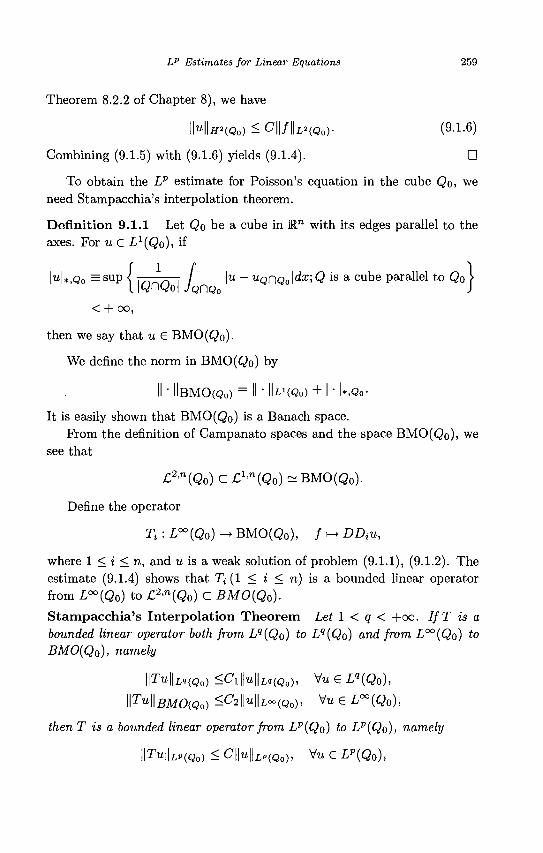
Lp Estimates for Linear Equations 259
Theorem 8.2.2 of Chapter 8), we have
IMIi/'Wo) ^ <?| | / | |L 2 ( Q o ) . (9.1.6)
Combining (9.1.5) with (9.1.6) yields (9.1.4). •
To obtain the LP estimate for Poisson's equation in the cube QQ, we need Stampacchia's interpolation theorem.
Definition 9.1.1 Let <3o be a cube in Rn with its edges parallel to the axes. For u € L1(Qo), if
|U|»,Q0 = sup \ / \u- UQDQO \dx\ <5 is a cube parallel to Q0 \ L \Qr\Qo\ JQC\QO J
< + oo,
then we say that u € BMO(<2o)' We define the norm in BMO(Qo) by
II ' llBMO(Qo) = II ' lU'CQo) + I • l*,Qo-
It is easily shown that BMO(Qo) is a Banach space. From the definition of Campanato spaces and the space BMO(Qo)> we
see that
£2 'n(Qo) C £1>n(Qo) - BMO(Qo)-
Define the operator
Ti : L°°(Q0) -» BMO(Qo), / •-» DDtu,
where 1 < i < n, and u is a weak solution of problem (9.1.1), (9.1.2). The estimate (9.1.4) shows that Tt (1 < i < n) is a bounded linear operator from L°°(Q0) to C2'n(Q0) C BMO(Q0). Stampacchia's Interpolation Theorem Let 1 < q < +oo. If T is a
bounded linear operator both from Lq(Qo) to Lq(Qo) and from L°°(Qo) to BMO(Q0), namely
| |Tu| |L ,W o ) <Ci | |u | | L , W o ) , Vu e L"{Q0),
WTU\\BMO(Q0) <^2 | | « | |L"O ( Q 0 ) , VU G L°° (QO) ,
then T is a bounded linear operator from Lp(Qo) to Lp(Qo), namely
\\Tu\\LHQo) < C | | « | | L P ( Q O ) I Vu e Lp(Q0),
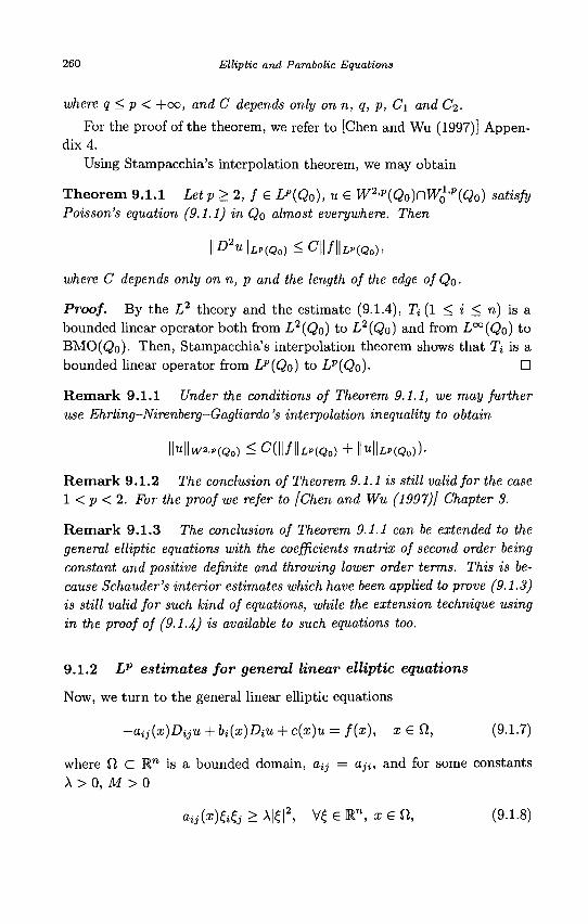
260 Elliptic and Parabolic Equations
where q < p < +00, and C depends only on n, q, p, C\ and C2 •
For the proof of the theorem, we refer to [Chen and Wu (1997)] Appendix 4.
Using Stampacchia's interpolation theorem, we may obtain
Theorem 9.1.1 Letp>2,fe LP(Q0), U £ W2'P(Q0)nW^'p(Q0) satisfy Poisson's equation (9.1.1) in Qo almost everywhere. Then
\\D2U\\LHQO) < C| | / | | iPW o) ,
where C depends only on n, p and the length of the edge of Qo •
Proof. By the L2 theory and the estimate (9.1.4), T; (1 < i < n) is a bounded linear operator both from L2(Qo) to L2(Qo) and from L°°(QQ) to BMO(<5o). Then, Stampacchia's interpolation theorem shows that Tj is a bounded linear operator from Lp(Qo) to Lp(Qo). •
Remark 9.1.1 Under the conditions of Theorem 9.1.1, we may further use Ehrling-Nirenberg-Gagliardo's interpolation inequality to obtain
\\u\\w2.r(Q0) < C(II/IILP(Q0) + IMUp(Qo))-
Remark 9.1.2 The conclusion of Theorem 9.1.1 is still valid for the case 1 < p < 2. For the proof we refer to [Chen and Wu (1997)] Chapter 3.
Remark 9.1.3 The conclusion of Theorem 9.1.1 can be extended to the general elliptic equations with the coefficients matrix of second order being constant and positive definite and throwing lower order terms. This is because Schauder's interior estimates which have been applied to prove (9.1.3) is still valid for such kind of equations, while the extension technique using in the proof of (9.1.4) is available to such equations too.
9.1.2 Lp estimates for general linear elliptic equations
Now, we turn to the general linear elliptic equations
-aij(x)Diju + bi(x)Diu + c(x)u = f(x), xeCl, (9.1.7)
where fi c R" is a bounded domain, ay = a,-,, and for some constants A > 0, M > 0
OijixMj > A|£|2, V£ £ f , x e fi, (9.1.8)
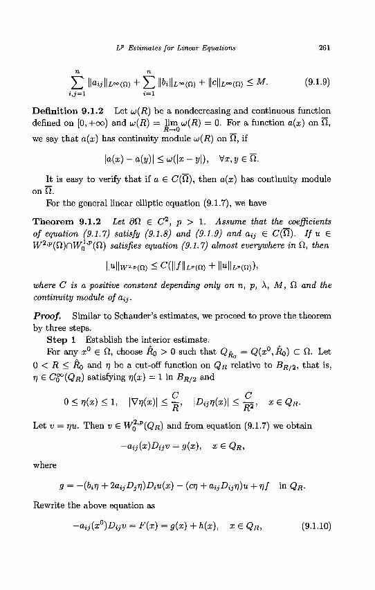
LP Estimates for Linear Equations 261
$ 3 IKIU°°(n) + Yl INU~(n) + l|c||L~(n) < M. (9.1.9) i,j = l i=l
Definition 9.1.2 Let w(i?) be a nondecreasing and continuous function defined on [0, +oo) and u(R) = lim u>(R) = 0. For a function a(x) on £2,
R—*-0 we say that a(x) has continuity module u(R) on £2, if
\a(x) -a(y)\ < w(\x-y\), Vx,y&Q.
It is easy to verify that if a £ C(O), then a(x) has continuity module on Q.
For the general linear elliptic equation (9.1.7), we have
Theorem 9.1.2 Let dCl G C2, p > 1. Assume that the coefficients of equation (9.1.7) satisfy (9.1.8) and (9.1.9) and a^ G C(fi). If u G W2,p(fi)nW0 'p(fi) satisfies equation (9.1.7) almost everywhere in £1, then
\\u\\w**p(n) < C(\\f \\Lp{n) + ||u||LP(n)),
where C is a positive constant depending only on n, p, X, M, Q, and the continuity module of a^-.
Proof. Similar to Schauder's estimates, we proceed to prove the theorem by three steps.
Step 1 Establish the interior estimate. For any x° £ Cl, choose Ro > 0 such that QR = Q(x°,Ro) C Cl. Let
0 < R < Ro and 77 be a cut-off function on QR relative to BR/2, that is, 77 G C$°{QR) satisfying rj(x) = 1 in BR/2 and
0 < ! 7 ( z ) < l , | V j j ( a O I < | . \DiM*)\ ^ §2> xeQR.
Let v = r\u. Then v G W0'P(QR) and from equation (9.1.7) we obtain
-aij(x)Dijv = g(x), x G QR,
where
g = -{hrj + 2aijDjrf)Diu{x) - (crj + a ^ D y ^ u + 77/ in QR.
Rewrite the above equation as
-aij(x°)Dijv = F(x)=g(x) + h(x), x G QR, (9.1.10)
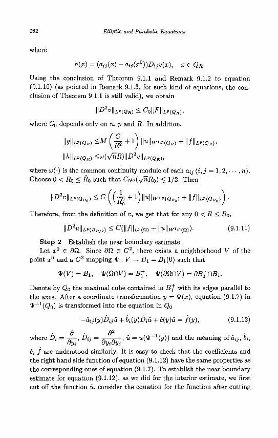
262 Elliptic and Parabolic Equations
where
h(x) = (ay(x) - ay(o:0))Aju(x), x e Qij.
Using the conclusion of Theorem 9.1.1 and Remark 9.1.2 to equation (9.1.10) (as pointed in Remark 9.1.3, for such kind of equations, the conclusion of Theorem 9.1.1 is still valid), we obtain
\\D2V\\LP(QR) < C 0 | | F | | L P ( Q f l ) ,
where Co depends only on n, p and R. In addition,
IISIILP(QR) <M \jp + 1 J llUlki.P(QR) + H/ | |LP(Q„),
II^IUP(OH) < W ( \ / ^ ) P 2 ^ I U » > ( Q H ) >
where w(-) is the common continuity module of each a,ij (i, j = 1,2, • • • , n). Choose 0 < .Ro < &o such that Cow(v/ni?o) < 1/2. Then
P^IU'WBO) ^ c ( ( 2 + ^hll^'noflo) + ll/lli'(OHo)J •
Therefore, from the definition of v, we get that for any 0 < R < Ro,
\\D2U\\LP(BR/2) < C( | | / | |Lp ( n ) + ||u||wi.,(n)). (9.1.11)
Step 2 Establish the near boundary estimate. Let x° e dQ. Since <9fl S C2 , there exists a neighborhood V of the
point x° and a C 2 mapping $ : V —> Bi = Bi(0) such that
*(V) = Bi, v(£inv) = B+, v(danv) = dBfnB1.
Denote by Qo the maximal cube contained in B^ with its edges parallel to the axes. After a coordinate transformation y = 9(x), equation (9.1.7) in ^~1(Qo) is transformed into the equation in Qo
- ay ( j / )Aj« + bi(y)DiU + c(y)u = f{y), (9.1.12)
d - d2
where Di = ——, Da = ——-—, u = uf^ :(j/)) and the meaning of au, bi, dyi dyidyj
c, f are understood similarly. It is easy to check that the coefficients and the right hand side function of equation (9.1.12) have the same properties as the corresponding ones of equation (9.1.7). To establish the near boundary estimate for equation (9.1.12), as we did for the interior estimate, we first cut off the function u, consider the equation for the function after cutting
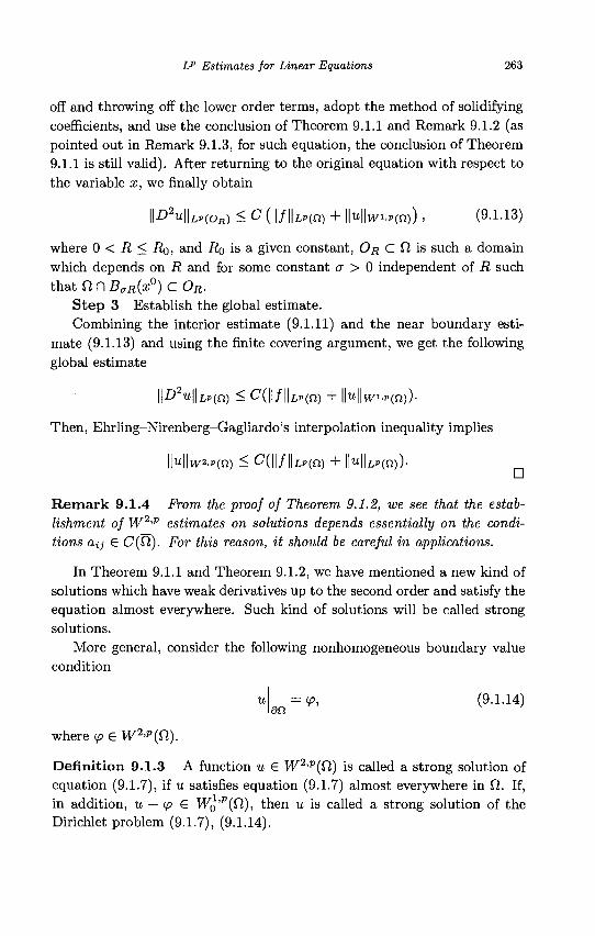
Lp Estimates for Linear Equations 263
off and throwing off the lower order terms, adopt the method of solidifying coefficients, and use the conclusion of Theorem 9.1.1 and Remark 9.1.2 (as pointed out in Remark 9.1.3, for such equation, the conclusion of Theorem 9.1.1 is still valid). After returning to the original equation with respect to the variable x, we finally obtain
\\D2U\\LP{0R) < C (||/||iP(n) + ll«lki.p(n)) , (9.1-13)
where 0 < R < R0, and Ro is a given constant, OR C il is such a domain which depends on R and for some constant a > 0 independent of R such that ft n BaR(xQ) C 0R.
Step 3 Establish the global estimate. Combining the interior estimate (9.1.11) and the near boundary esti
mate (9.1.13) and using the finite covering argument, we get the following global estimate
||D2uj|£p(n) < C(||/| |Lp (n) + IMIwn.p(n)).
Then, Ehrling-Nirenberg-Gagliardo's interpolation inequality implies
||w||vK2.p(n) < C(||/| |LP(n) + ||u||ip(n)).
Remark 9.1.4 From the proof of Theorem 9.1.2, we see that the establishment of W2'p estimates on solutions depends essentially on the conditions a,ij € C(fl). For this reason, it should be careful in applications.
In Theorem 9.1.1 and Theorem 9.1.2, we have mentioned a new kind of solutions which have weak derivatives up to the second order and satisfy the equation almost everywhere. Such kind of solutions will be called strong solutions.
More general, consider the following nonhomogeneous boundary value condition
u fln^' ( 9 - L 1 4 )
where <p e W2'P(Q).
Definition 9.1.3 A function u G W2'P(Q) is called a strong solution of equation (9.1.7), if u satisfies equation (9.1.7) almost everywhere in Q. If, in addition, u — ip £ W0
1,P(Q), then u is called a strong solution of the Dirichlet problem (9.1.7), (9.1.14).
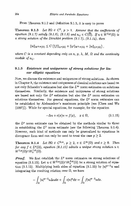
264 Elliptic and Parabolic Equations
Prom Theorem 9.1.2 and Definition 9.1.3, it is easy to prove
Theorem 9.1.3 Let dfl G C2, p > 1. Assume that the coefficients of equation (9.1.7) satisfy (9.1.8), (9.1.9) and ay G C(ty. If u G W2>p(Ct) is a strong solution of the Dirichlet problem (9.1.7), (9.1.14), then
||u||w2.p(n) < C (||/||Lp(n) + IMIw«.p(n) + IMUp(n)),
where C is a constant depending only on n, p, X, M, fl and the continuity module of aij.
9.1.3 Existence and uniqueness of strong solutions for linear elliptic equations
Now, we discuss the existence and uniqueness of strong solutions. As shown in Chapter 8, the existence and uniqueness of classical solutions are based on not only Schauder's estimates but also the L°° norm estimates on solutions themselves. Similarly, the existence and uniqueness of strong solutions are based not only the LP estimates but also the Lp norm estimates on solutions themselves. For general equations, the Lp norm estimates can be established by Aleksandrov's maximum principle (see [Chen and Wu (1997)]). While for special equations, for example, for the equation
-Au + c(x)u = f(x), xGf i , (9.1.15)
the Lp norm estimate can be obtained by the methods similar to those in establishing the L2 norm estimate (see the following Theorem 9.1.4). However, such kind of methods can only be generalized to equations in divergence form and can only be used to treat the case p > 2.
Theorem 9.1.4 Let dQ G C2>a, p > 2, c G L°°(fi) and c > 0. Then for any f G Lp(Cl), equation (9.1.15) admits a unique strong solution u G
w2>p(n)nwt>p(n). Proof. We first establish the LP norm estimates on strong solutions of equation (9.1.15). Let u G W2>P{Q)PWQ'V{SI) be a strong solution of equation (9.1.15). Multiplying both sides of equation (9.1.15) by |u | p _ 2u and integrating the resulting relation over Q,, we have
— / \u\p~2uAudx + / c|u|pda; = / f\u\p~~2udx. Ja Jo, Jn
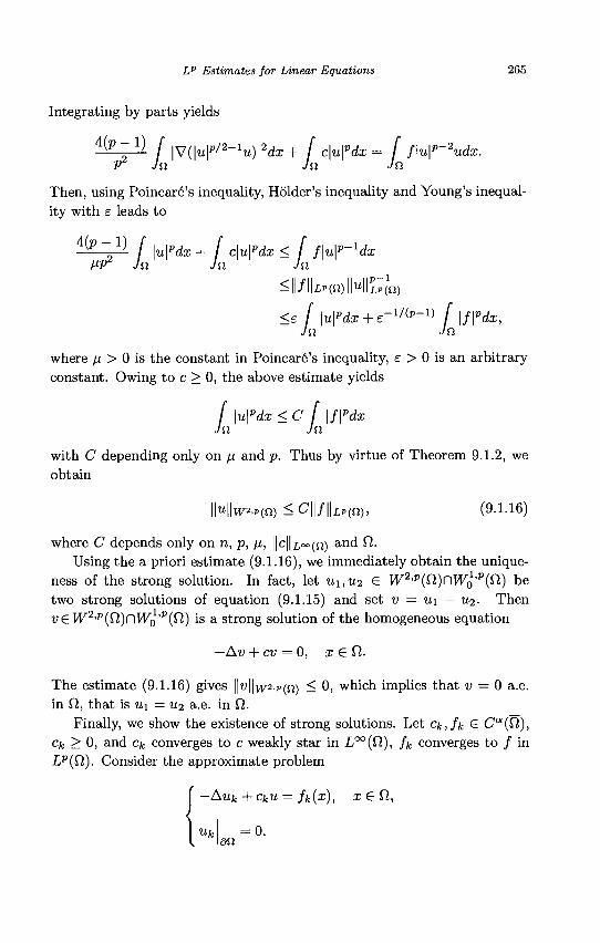
Lp Estimates for Linear Equations 265
Integrating by parts yields
4(P - 1) p2
/ |V(|u|p /2-1u)|2da;+ f c\u\pdx = f f\u\p~2udx. Jn Jn Jn
Then, using Poincare's inequality, Holder's inequality and Young's inequality with e leads to
4(P ~ 1) fip2
I \u\pdx + f c\u\pdx < f flu^dx Jn Jn Jn
<\\f\\r,P(m\\u IP—i LP(n) | | " l lL P ( n)
<£ / \u\pdx + e-1/{p-l) [ \f\pdx, Jn Jn
where ji > 0 is the constant in Poincare's inequality, e > 0 is an arbitrary constant. Owing to c > 0, the above estimate yields
/ \u\pdx <C [ \f\pda Jn Jn
with C depending only on /j, and p. Thus by virtue of Theorem 9.1.2, we obtain
\Hw*.r(n) < C||/ |Up (n )> (9.1.16)
where C depends only on n, p, /u, ||c||ioo(n) and ^-Using the a priori estimate (9.1.16), we immediately obtain the unique
ness of the strong solution. In fact, let ui,U2 £ W2'p(D,)r\W0'p(Cl) be
two strong solutions of equation (9.1.15) and set v = u\ — u^. Then v£ W2'P(D.)C)WQ'P(Q.) is a strong solution of the homogeneous equation
—Av + cv = 0, x £ D,.
The estimate (9.1.16) gives \\v\\w2-"(n) 5= 0, which implies that v = 0 a.e. in Q, that is u\ = u<i a.e. in fi.
Finally, we show the existence of strong solutions. Let Ck,fk € Ca(fi), Cfe > 0, and Cfe converges to c weakly star in L°°(fl), fk converges to / in Lp(Cl). Consider the approximate problem
-Auk + cku = fk{x), i G f l ,
Ufe = 0 . a n
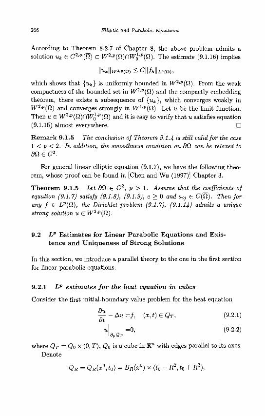
266 Elliptic and Parabolic Equations
According to Theorem 8.2.7 of Chapter 8, the above problem admits a solution uk G C2'a(U) c W2 'p(fi)rW0
1,p(ft). The estimate (9.1.16) implies
||wfc||w2.p(n) < C||/fe|Up(n),
which shows that {uk} is uniformly bounded in W2'p(fl). Prom the weak compactness of the bounded set in W2'P(Q) and the compactly embedding theorem, there exists a subsequence of {ufc}, which converges weakly in W2'p(Cl) and converges strongly in W1,p(fi). Let u be the limit function. Then u G W2>p(£l)r\W0
1'p(Q) and it is easy to verify that u satisfies equation (9.1.15) almost everywhere. •
Remark 9.1.5 The conclusion of Theorem 9.1.4 is still valid for the case 1 < p < 2. In addition, the smoothness condition on dCl can be relaxed to dSl G C2.
For general linear elliptic equation (9.1.7), we have the following theorem, whose proof can be found in [Chen and Wu (1997)] Chapter 3.
Theorem 9.1.5 Let dQ G C2, p > 1. Assume that the coefficients of equation (9.1.7) satisfy (9.1.8), (9.1.9), c > 0 and atj G C(Q). Then for any f G LP(Q), the Dirichlet problem (9.1.7), (9.1.14) admits a unique strong solution u G W2'P{Q).
9.2 Lp Estimates for Linear Parabolic Equations and Existence and Uniqueness of Strong Solutions
In this section, we introduce a parallel theory to the one in the first section for linear parabolic equations.
9.2.1 Lp estimates for the heat equation in cubes
Consider the first initial-boundary value problem for the heat equation
Fin ^-Au=f, (x,t)eQT, (9.2.1)
u =0, (9.2.2) dpQr
where QT — Qo x (0, T), Q0 is a cube in W1 with edges parallel to its axes. Denote
QR = QR(X°, t0) = BR(x°) x (t0 - R2, t0 + R2),
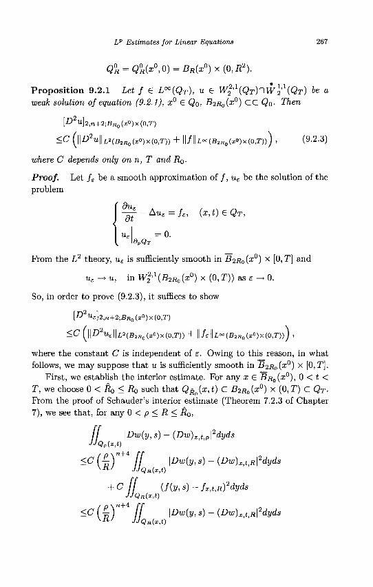
Lp Estimates for Linear Equations 267
QR = QR(X°,0) = BR(X°)X(0,R2).
Proposi t ion 9.2.1 Let f G L°°(QT), u G Wl'l{QT)r\w\'l{QT) be a weak solution of equation (9.2.1), x° G Qo, B2R0(x°) CC QO- Then
[D u]2,n+2;BH o(x°)x(0,T)
<C (\\D2U\\L2{B2RQ{XO)X{0,T)) + | | / | | L ° ° ( B 2 H O ( X ° ) X ( 0
where C depends only on n, T and RQ .
,T))) , (9.2.3)
Proof. Let fe be a smooth approximation of / , ue be the solution of the problem
Oil
—£• - Aue = /E , (x, t) G QT,
= 0. dpQr
From the L2 theory, ue is sufficiently smooth in B2R0{x°) X [0,T] and
u£ - • u, in W22,1(B2Ro(a;0) x (0,T)) as e -» 0.
So, in order to prove (9.2.3), it suffices to show
\D2 UE}2>n+2iBRo (x<>) x (0,T)
<C ^|]£>2UE | |L2(B2Ro(xO)x(0,T)) + | | /elti«»(B2„0(xO)x(0,r))_) ,
where the constant C is independent of e. Owing to this reason, in what follows, we may suppose that u is sufficiently smooth in B2R0(x°) X [0,T].
First, we establish the interior estimate. For any x G BR0(X°), 0 < t < T, we choose 0 < Ro < Ro such that QRo(x,t) C B2R0(X°) X (0,T) C QT-
From the proof of Schauder's interior estimate (Theorem 7.2.3 of Chapter 7), we see that, for any 0 < p < R < Ro,
I Qp(x,t) \Dw(y,s) - (Dw)XitJ
2dyds
<C
<C
+cii JjQR(x
org
\Dw(y, s) - {Dw)x,t,R\2dyds Qa(x,t)
(f(y, s) - fx,t,R)2dyds t)
Qs( i , t ) \Dw(y,s) - (Dw)x^R\2dyds
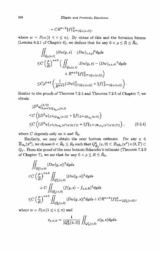
268 Elliptic and Parabolic Equations
+ CRn ||/|lz,~(Q„(x,t))'
where w = Diu{l < i < n). By virtue of this and the iteration lemma (Lemma 6.2.1 of Chapter 6), we deduce that for any 0 < p < R < Ro,
\±sujyy,oj — {j_sui)xj,p\ Qp(x,t)
\Dw(y,s) - (Dw)xAp\2dyds
<C ( £ ) " + 2 ( ff \Dw(y, s) - {Dw)x^R\2dyds V -K / KJjQR(x,t)
+ Rn+2\\f\\UQR(x,t)))
^pn+2 (^+2 \\^\\h{QRix>t)) + ii/iii-Wj,(..t))
Similar to the proofs of Theorem 7.2.4 and Theorem 7.2.5 of Chapter 7, we obtain
\-u Uh,n+2;Qko/2(x,t)
<C (\\D2u\\L2(Qko{x,t)) + ||/||z,°°(QAo(x,t)))
<C [\\D2u\\L2{B2RQ{xo)x{0tT)) + | | / | |L°°(B2RO(X°)X(O,T))J , (9.2.4)
where C depends only on n and Ro. Similarly, we may obtain the near bottom estimate. For any x £
5 f l o (x°), we choose 0 < Ro < Ro such that Q°R (x, 0) C B2Ro (x°) x (0, T) C QT- From the proof of the near bottom Schauder's estimate (Theorem 7.2.9 of Chapter 7), we see that for any 0 < p < R < Ro,
I \Dw(y,s)\ dyds Q?(».o)
- C ( l ) " + 4 / / o \Dw(y,s)\2dyds
+ C ff (f(y,s)-fx,0,R)2dyds JJQ°R(X,O)
<c(L)n+i ff \Dw(y,s)\2dyds + CRn+2\\f\\l„{QO,0)), ^R' JJQ°(X,O) R IQ°R(X,0)
where w = DiU (1 < i < n) and
VX,O,R = l n 0 , n M / / v(y, s)dyd,
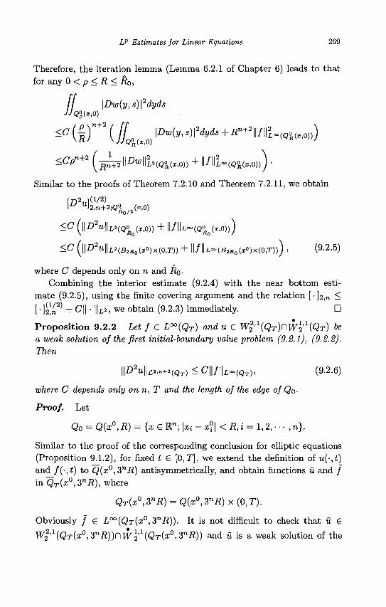
LP Estimates for Linear Equations 269
Therefore, the iteration lemma (Lemma 6.2.1 of Chapter 6) leads to that for any 0 < p < R < Ro,
\Dw(y,s)\2dyds Q°(x,0)
-c(l)n+2(i/'o x0 \D™(y>s)\2dyds + Rn+2\\f\\l~(Q%(X,o^
<CPn+2 ( ] ^ I M l i ' ( Q i < . . 0 ) ) + H/ll£-(Q4(„0))
Similar to the proofs of Theorem 7.2.10 and Theorem 7.2.11, we obtain
[£> 2 i / l ( 1 / 2 )
\-U Uh,n+2;Qlo/2(x,0)
<C ^||£»2u||L2(Q^(X)0)) + II/IIL~(Q^O(X,O))J
<C [\\D2u\\L2(B2Ro(xo)X(0iT)) + | | / | |L~(B2RO(XO)X(O,T))J . (9.2.5)
where C depends only on n and Ro. Combining the interior estimate (9.2.4) with the near bottom esti
mate (9.2.5), using the finite covering argument and the relation [-]2,n < [ • ){2,L2) + C|| • ||L2, we obtain (9.2.3) immediately. D Proposition 9.2.2 Let f G L°°(QT) and u e W%'1 {QT)C\w\'1 {QT) be a weak solution of the first initial-boundary value problem (9.2.1), (9.2.2). Then
\\D2u\\c2,n+HQT) < C | | / | | i« ,W T ) > (9.2.6)
where C depends only on n, T and the length of the edge of QQ.
Proof. Let
Qo = Q(x°,R) = {x£Wl;\xi-x°i\ < R,i = 1,2, • • • , n} .
Similar to the proof of the corresponding conclusion for elliptic equations (Proposition 9.1.2), for fixed t G [0,T], we extend the definition of u(-,t) and f(-,t) to Q(x°,3nR) antisymmetrically, and obtain functions u and / inQT(a;0 ,3n i?), where
QT(x°,3nR) = Q(x°,3nR) x (0,T).
Obviously / G L°°(QT(x°, 3nR)). It is not difficult to check that u G
Wl'l(QT(x0,3nR))r\W2l{QT{x°,3nR)) and u is a weak solution of the
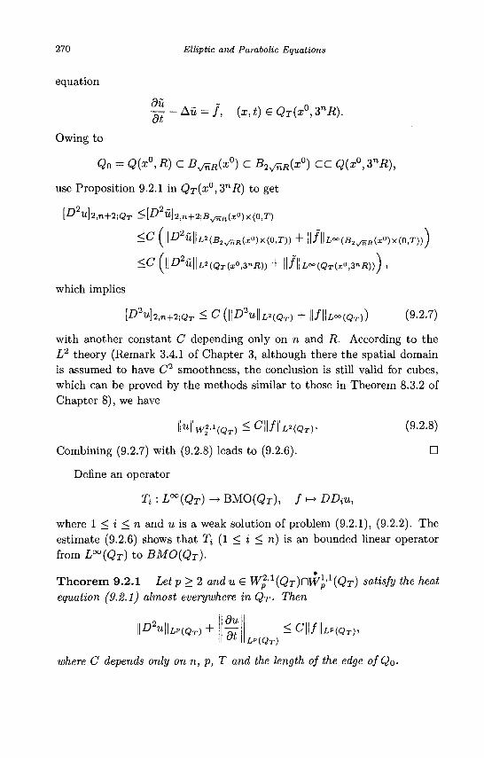
270 Elliptic and Parabolic Equations
equation
3v ~ ^ - A u = / , (x,t)GQT(x°,3nR).
Owing to
Qo = Q(x°,R) C B^R(x°) c B2VER(x°) CC Q(x°,3nR),
use Proposition 9.2.1 in QT(x°,3nR) to get
[£> U]2 ,n+2;QT <[D u}2,n+2;Bv7[R(x0)x(0,T)
<C (\\D2u\\L2(B2V__Hix0)x{0,T)) + | | / | |L- (S 2 v / i j f i (xO)x(0 ,T)) )
<C ^ | | Z ) 2 ' U | | Z , 2 ( Q T ( a . 0 ] 3 r l f i ) ) + | | / | | i o o ( Q r ( x 0 i 3 n j R ) ) J ,
which implies
[D2u}2tn+2]Ql. < C (\\D2U\\L2{QT) + | | / | | L O O ( Q T ) ) (9.2.7)
with another constant C depending only on n and R. According to the L2 theory (Remark 3.4.1 of Chapter 3, although there the spatial domain is assumed to have C2 smoothness, the conclusion is still valid for cubes, which can be proved by the methods similar to those in Theorem 8.3.2 of Chapter 8), we have
\Hwli(QT)<C\\f\\LHQT). (9.2.8)
Combining (9.2.7) with (9.2.8) leads to (9.2.6). •
Define an operator
T i : L o o ( Q T ) - . B M 0 ( g T ) , / >-> DDtu,
where 1 < i < n and u is a weak solution of problem (9.2.1), (9.2.2). The estimate (9.2.6) shows that Tj (1 < i < n) is an bounded linear operator from L°°(QT) to BMO(QT).
Theorem 9.2.1 Letp>2 and u G W2'1 {QT)^Wl'x (QT) satisfy the heat equation (9.2.1) almost everywhere in QT- Then
\D2U\\LV{QT) du It <C\\f\\LnQT),
LP(QT)
where C depends only on n, p, T and the length of the edge of QQ.
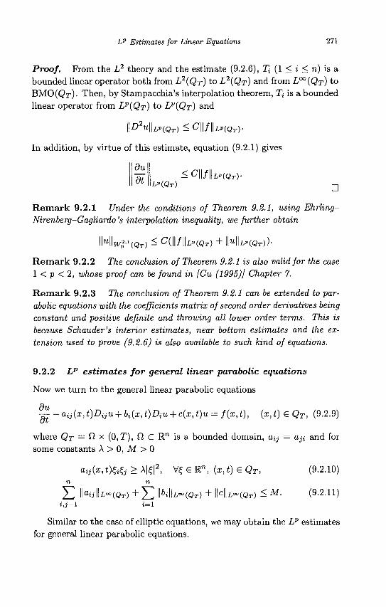
Lp Estimates for Linear Equations 271
Proof. Prom the L? theory and the estimate (9.2.6), Tt (1 < i < n) is a bounded linear operator both from L2(QT) to L2(QT) and from L°°(QT) to B M O ( Q T ) - Then, by Stampacchia's interpolation theorem, Tj is a bounded linear operator from LP(QT) to LP(QT) and
\\D2u\\Lv{QT)<C\\f\\LHQT).
In addition, by virtue of this estimate, equation (9.2.1) gives
du < C | | / | | L P ( Q T ) .
L"(QT) D
Remark 9.2.1 Under the conditions of Theorem 9.2.1, using Ehrling-Nirenberg-Gagliardo 's interpolation inequality, we further obtain
\\U\\W2,I{QT) < C(\\f\\Lp{QT) + | | U | | L P « M ) -
Remark 9.2.2 The conclusion of Theorem 9.2.1 is also valid for the case 1 < p < 2, whose proof can be found in [Gu (1995)J Chapter 7.
Remark 9.2.3 The conclusion of Theorem 9.2.1 can be extended to parabolic equations with the coefficients matrix of second order derivatives being constant and positive definite and throwing all lower order terms. This is because Schauder's interior estimates, near bottom estimates and the extension used to prove (9.2.6) is also available to such kind of equations.
9.2.2 Lp estimates for general linear parabolic equations
Now we turn to the general linear parabolic equations
du — -aij(x,t)DijU + bi(x,t)DiU + c(x,t)u = f(x,t), (x,t) <E QT, (9.2.9)
where QT = ^ x (0,T), Q, c M" is a bounded domain, ay = a^ and for some constants A > 0, M > 0
M M ) & & > A | £ | 2 , V f e R n , M e Q r , (9-2.10) n n
J2 Hay IU~«JT) + 5Z INU~(QT) + ||C||L~(QT) ^ M- (9.2.11) i,j = l i = l
Similar to the case of elliptic equations, we may obtain the LP estimates for general linear parabolic equations.
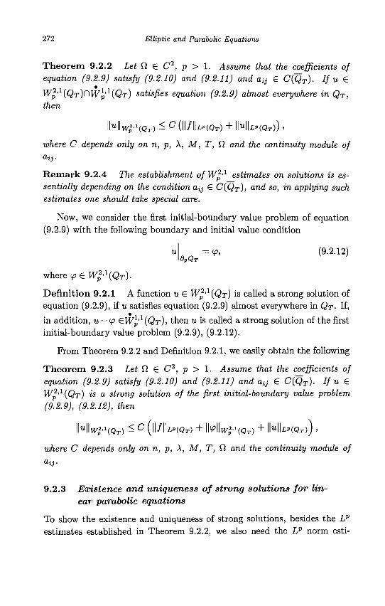
272 Elliptic and Parabolic Equations
Theorem 9.2.2 Let fi £ C2, p > 1. Assume that the coefficients of equation (9.2.9) satisfy (9.2.10) and (9.2.11) and aij £ C(QT). If u £
W2'1 (QT)^WJ,'1 (QT) satisfies equation (9.2.9) almost everywhere in QT,
then
Hwtf- 'Wr) - C(\\fh"(QT) + \\U\\LP(QT)) ,
where C depends only on n, p, X, M, T, fi and the continuity module of
Remark 9.2.4 The establishment of Wp'1 estimates on solutions is essentially depending on the condition a^ £ C(QT), and so, in applying such estimates one should take special care.
Now, we consider the first initial-boundary value problem of equation (9.2.9) with the following boundary and initial value condition
. =¥>, (9-2.12) OPQT
where <p £ W2'1(QT).
Definition 9.2.1 A function u £ Wp'1(Qx) is called a strong solution of equation (9.2.9), if u satisfies equation (9.2.9) almost everywhere in QT- If,
* in addition, u — <p £Wp (QT), then u is called a strong solution of the first
initial-boundary value problem (9.2.9), (9.2.12).
Prom Theorem 9.2.2 and Definition 9.2.1, we easily obtain the following
Theorem 9.2.3 Let Q £ C2, p > 1. Assume that the coefficients of equation (9.2.9) satisfy (9.2.10) and (9.2.11) and ay £ C{QT). If u £ W2,1(QT) is a strong solution of the first initial-boundary value problem (9.2.9), (9.2.12), then
Wu\\w$'\QT) ^ C (|I/IU"(OT) + IMIWI'^QT) + IMU»(QT)) .
where C depends only on n, p, X, M, T, Q, and the continuity module of
9.2.3 Existence and uniqueness of strong solutions for linear parabolic equations
To show the existence and uniqueness of strong solutions, besides the Lp
estimates established in Theorem 9.2.2, we also need the U norm esti-
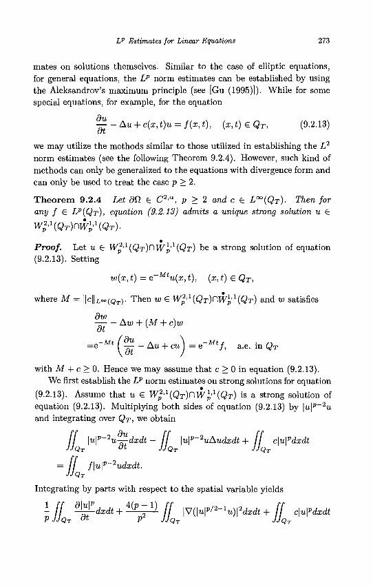
Lp Estimates for Linear Equations 273
mates on solutions themselves. Similar to the case of elliptic equations, for general equations, the Lp norm estimates can be established by using the Aleksandrov's maximum principle (see [Gu (1995)]). While for some special equations, for example, for the equation
3u — -Au + c{x,t)u = f(x,t), (x,t)EQT, (9.2.13)
we may utilize the methods similar to those utilized in establishing the L2
norm estimates (see the following Theorem 9.2.4). However, such kind of methods can only be generalized to the equations with divergence form and can only be used to treat the case p > 2.
Theorem 9.2.4 Let dQ G C2'a, p > 2 and c G L°°{QT). Then for any f G LP(QT), equation (9.2.13) admits a unique strong solution u G
Proof. Let u G W2'1(QT)<~\WI'1{QT) be a strong solution of equation (9.2.13). Setting
w(x,t)=e-mu{x,t), {x,t)eQT,
where M = \\C\\L*°(QT). Then w G W2A (Qr)rWp'1 (QT) and w satisfies
9w . . , , . — Aw + (M + c)w at
=e~m (J^-Au + cu\ = e~Mtf, a.e. in QT
with M + c > 0. Hence we may assume that c > 0 in equation (9.2.13). We first establish the Lp norm estimates on strong solutions for equation
(9.2.13). Assume that u G W2'1 (QT)r)Wl'1 (QT) is a strong solution of equation (9.2.13). Multiplying both sides of equation (9.2.13) by |w|p_2w and integrating over QT, we obtain
/ / \u\p-2u-^dxdt - jf \u\p'2uAudxdt + ff c\u\pdxdt
= If f\u\p~2udxdt. JJQT
Integrating by parts with respect to the spatial variable yields
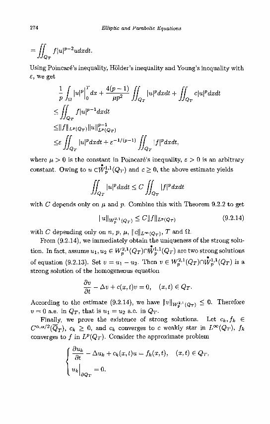
274 Elliptic and Parabolic Equations
I f\u\p-2udxdt. QT
Using Poincare's inequality, Holder's inequality and Young's inequality with e, we get
- / \u\p Tdx + 1 ^ — H / / \u\pdxdt + ff c\u\pdxdt
PJn o MP2 JJQT JJQT
<ff f\u\p-lc IQT JJQT
ldxdt
^II/IIL»«T)IIUIILP(QT)
< £ ff \u\pdxdt + e-ltto-V ff \f\vdxdt, JJQT JJQT
where /x > 0 is the constant in Poincare's inequality, e > 0 is an arbitrary
constant. Owing to u €.W),'1{QT) and c > 0, the above estimate yields
/ / \u\pdxdt <C ff \f\pdxdt JJQT JJQT IQT JJQJ
with C depends only on /x and p. Combine this with Theorem 9.2.2 to get
N I ^ . 1 ( Q T ) < C | | / | | L P ( Q T ) (9.2.14)
with C depending only on n, p, /x, ||C||/,<=O(QT), T and f2.
From (9.2.14), we immediately obtain the uniqueness of the strong solu
tion. In fact, assume u\, u-i G W2'1 (QT)CWI'1 (QT) are two strong solutions
of equation (9.2.13). Set v = ui - u2. Then v G W^1 (QT^W1/[QT) is a
strong solution of the homogeneous equation
Ov — -Av + c(x,t)v = 0, (x,t)GQT-
According to the estimate (9.2.14), we have ||«||wa'1(Qr) ^ 0- Therefore v = 0 a.e. in QT, that is ux = it2 a.e. in QT-
Finally, we prove the existence of strong solutions. Let ck,fk 6 Ca'a/2(QT), Ck > 0, and ck converges to c weakly star in L°°(QT), fk converges to / in LP(QT)- Consider the approximate problem
— - Aufc +ck(x,t)u = fk(x,t), (x,t) G QT,
Uk = 0. dQT
LP Estimates for Linear Equations 275
According to Theorem 8.3.7 of Chapter 8, the above problem admits a solution Uk G C2'a(QT). Thus the estimate (9.2.14) gives
I N H W ^ Q T ) - CWfk\\LP(QT)'
which implies that {u^} is uniformly bounded in W2'1(QT). Prom the
weak compactness of the bounded set in W2'1(QT) and WP'1{QT) and the compactly embedding theorem, there exists a subsequence of {wfe},
which converges weakly in W2'1(QT) and Wp^iQr), and converges strongly in LP(QT). Let u be the limit function. It is easy to verify that u G Wp'1 (QT)^W);1 (QT) and u satisfies equation (9.2.13) almost everywhere in QT. •
Remark 9.2.5 Different from the case of elliptic equations (Theorem 9.2-4)> the restriction condition c > 0 is not required.
Remark 9.2.6 The conclusion of Theorem 9.2.4 is still valid for the case 1 < p < 2. In addition, it suffices to require dfl G C2.
For general linear parabolic equation (9.2.9), we have the following theorem, whose proof can be found in [Gu (1995)] Chapter 7.
Theorem 9.2.5 Let dCl G C2, p > 1. Assume that the coefficients of equation (9.2.9) satisfy (9.2.10) and (9.2.11), and a^ G C{QT). Then for any f £ LP(QT), the first initial-boundary value problem (9.2.9), (9.2.12) admits a unique strong solution u € W2'1 (QT) •
Exercises
1. Check u G H2(Q(x°,3nR)) in Proposition 9.1.2, and judge whether the following arguments are valid:
i)IiueC1'a(Q(x°,R))&ndu Q = 0, thenu € C1'a(Q{x°,3nR));
ii) If u € C2(Q(x°, R)) and u = 0 , then u G H2(Q(x°, 3nR)). dQ(x°,R) _ V V "
2. Prove that a(x) has a continuity module in Q if and only if a(x) G C(£l), where CI is an bounded open set in R™.
3. Let CI C E™ be a bounded domain with appropriately smooth boundary, A G E, p > 1. Then there is one and only one of the following alternatives:
276 Elliptic and Parabolic Equations
i) The boundary value problem for the homogeneous equation
—Au + Xu = 0 in il, u an
0
admits a nontrivial strong solution u € W2'P(Q,) n WQ'P(CI);
ii) For any / e Lp(il), the boundary value problem for the inhomoge-neous equation
—Au + Xu = f in CI, u an
= 0
admits a unique strong solution u € W2'p{Cl) D W0'P(Q).
Chapter 10
Fixed Point Method
The approaches based on fixed point theorems have very important applications in the investigation of partial differential equations, especially the nonlinear differential equations. In this chapter, as an example, we apply such a method to the solvability of quasilinear elliptic equations.
10.1 Framework of Solving Quasilinear Equations via Fixed Point Method
In this section, we describe the basic framework of fixed point method in solving quasilinear equations.
10.1.1 Leray-Schauder's fixed point theorem
Leray-Schauder's Fixed Point Theorem Let U be a Banach space, T(u,a) be a mapping from Ux [0,1] to U satisfying the following conditions:
i) T is a compact mapping; ii) T{u, 0) = 0, \/u £ U; Hi) There exists a constant M > 0, such that for any u € U, if u =
T(u, a) for some a € [0,1], then \\u\\u < M. Then the mapping T(-, 1) has a fixed point, that is, there exists u G U,
such that u = T(u, 1).
10.1.2 Solvability of quasilinear elliptic equations
We first consider the Dirichlet problem for quasilinear elliptic equations
- diva(:r, u, Vw) + b(x, u, Vu) = 0, x € 9., (10.1.1)
277
278 Elliptic and Parabolic Equations
dQ = ¥>> (10.1.2)
where a = {a\, a<i, • • • ,an) and ft C W1 is a bounded domain. Assume that a{x,z,rj), b{x,z,rj) satisfy the following structure conditions:
OTjj
\a,i(x,z,Q)\ <g(x),
dai <ti\*\
dai
8z
dai
drij
+ |oi|<MN)(i + l'7l),
+ |6|<M(N)(1 + H2), dxj
-b(x, z, r])sgnz < A(\n\ + h(x)),
(10.1.3)
(10.1.4)
(10.1.5)
(10.1.6)
(10.1.7)
(10.1.8)
where i, j = 1,2, • • • ,n, X, A > 0, g € Lq(Cl)(q > n), h G L9*(0), q* nq/(n + q) and /x(s) is a nondecreasing function on [0, +oo).
A typical example of such equations satisfying (10.1.3)-(10.1.8) is
where
-div(a(u)Vu) + b(u) = f(x), x e ft,
o(u) = (u2 + l ) m / 2 (m > 0), b{u) = lu^u (7 > 1)
(10.1.9)
and / e Ca(ft). For simplicity, we consider only the Dirichlet problem with the homogeneous boundary value condition
an = 0. (10.1.10)
Theorem 10.1.1 Let 0 < a < 1, dfl € C2'a, a e C1'01, b € Ca, <p G C2'a(fl). Assume that the structure conditions (10.1.3)-(10.1.8) hold. Then
i) There exist a constant 0 < j3 < 1 and a constant M > 0 depending only onn, X, A, ||s||L«(n), ||/i||L«.(n)) Ks)> \fU,a-,n, \a\i,a, \b\a andfl, such that for any solution u G C2'a(fl) of problem (10.1.1), (10.1.2),
Ml,/3;fi < M;
M) Problem (10.1.1), (10.1.2) admits a solution u G C2'a{ft).
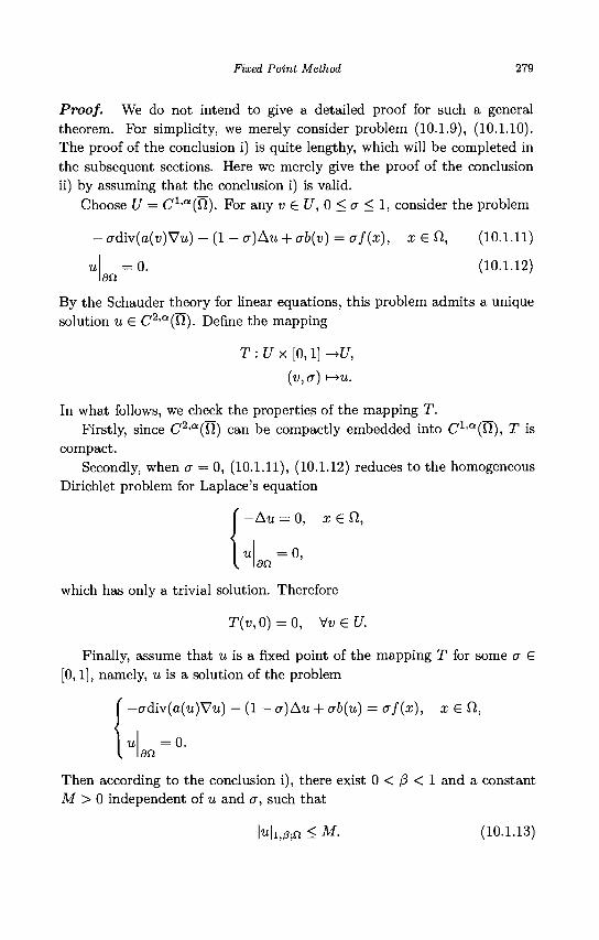
Fixed Point Method 279
Proof. We do not intend to give a detailed proof for such a general theorem. For simplicity, we merely consider problem (10.1.9), (10.1.10). The proof of the conclusion i) is quite lengthy, which will be completed in the subsequent sections. Here we merely give the proof of the conclusion ii) by assuming that the conclusion i) is valid.
Choose U = C1 , a(fi). For any v £ U, 0 <a <1, consider the problem
adiv(a(v)Vu) - (1 - a)Au + ab{v) = af(x), x £ Q,,
= 0. an
(10.1.11)
(10.1.12)
By the Schauder theory for linear equations, this problem admits a unique solution u £ C2'a(D.). Define the mapping
T : U x [0,1] -+C/,
(v,a) \-*u.
In what follows, we check the properties of the mapping T. Firstly, since C2 'a(fi) can be compactly embedded into C1 ,a(fi), T is
compact. Secondly, when a = 0, (10.1.11), (10.1.12) reduces to the homogeneous
Dirichlet problem for Laplace's equation
Au = 0, x £0,,
« = 0 > an
which has only a trivial solution. Therefore
T(u, 0 ) = 0 , Vv£U.
Finally, assume that u is a fixed point of the mapping T for some a £ [0,1], namely, u is a solution of the problem
crdiv(a(u)Vu) — (1 - a)Au + crb(u) = af(x), x £Cl,
= 0. an
Then according to the conclusion i), there exist 0 < (3 < 1 and a constant M > 0 independent of u and a, such that
|u|i,/3;n < M. (10.1.13)
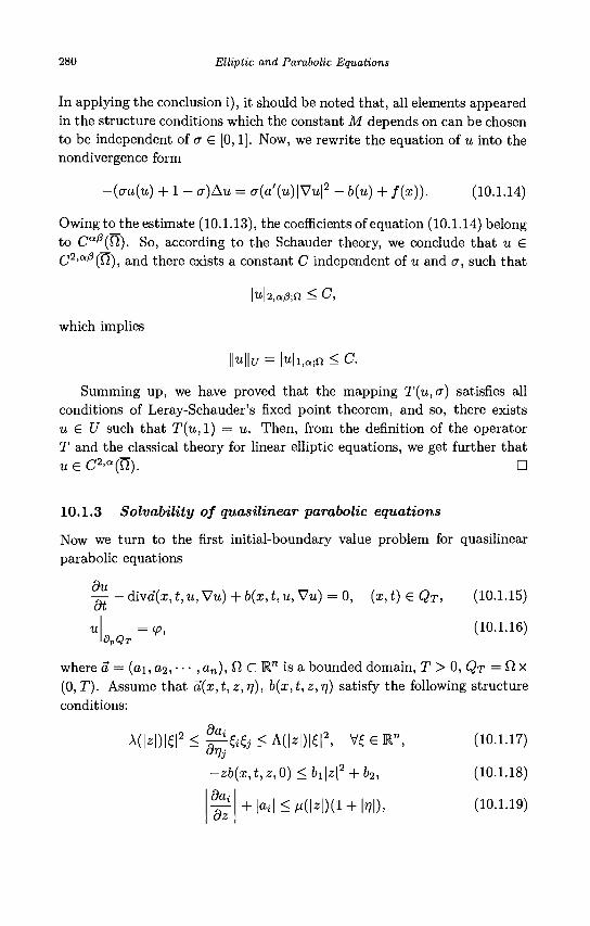
280 Elliptic and Parabolic Equations
In applying the conclusion i), it should be noted that, all elements appeared in the structure conditions which the constant M depends on can be chosen to be independent of a € [0,1]. Now, we rewrite the equation of u into the nondivergence form
-(aa(u) + 1 - a)Au = cr(a'(w)|Vu|2 - b(u) + f(x)). (10.1.14)
Owing to the estimate (10.1.13), the coefficients of equation (10.1.14) belong to Ca"(ft). So, according to the Schauder theory, we conclude that u S C2'af}(Q.), and there exists a constant C independent of u and a, such that
|w|2,a/3;0 < C,
which implies
||u||y = Ml,a;f2 < C.
Summing up, we have proved that the mapping T(u,a) satisfies all conditions of Leray-Schauder's fixed point theorem, and so, there exists u € U such that T(u, 1) = u. Then, from the definition of the operator T and the classical theory for linear elliptic equations, we get further that u£C2'a(ty. D
10.1.3 Solvability of quasilinear parabolic equations
Now we turn to the first initial-boundary value problem for quasilinear parabolic equations
du — - diva(x, t, u, Vu) + b(x, t, u, Vu) = 0, ( i , t ) e Q r , (10.1.15)
= <p, (10.1.16) dpQT
where a = (ai, 02, • • • , a n ) , Q, C M.n is a bounded domain, T > 0, QT = ft x (0,T). Assume that a(x,t,z,r)), b(x,t,z,rj) satisfy the following structure conditions:
A ( | z | ) | £ | 2 < ! ^ < A ( | 2 | ) | £ | 2 , V ^ e l " , (10.1.17)
-zb(x,t,z,0)<b1\z\2 + b2, (10.1.18)
den dz
jOi l^ / idzDa + M), (10.1.19)
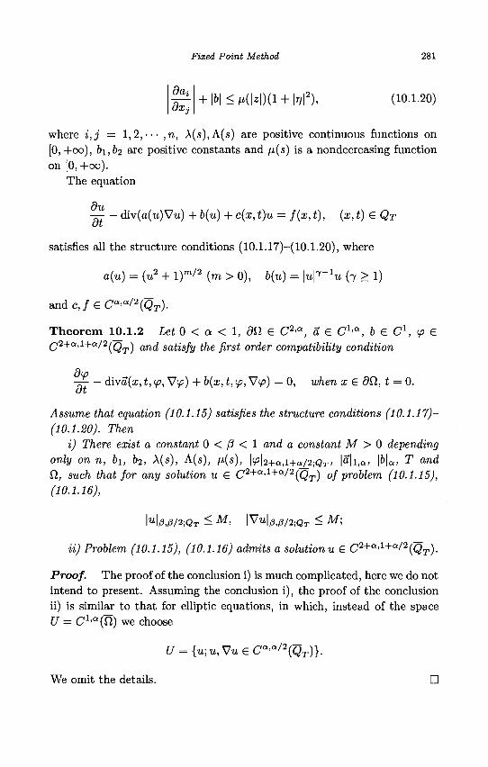
Fixed Point Method 281
da* dxj
+ | 6 | < M ( | Z | ) ( 1 + | T ? | 2 ) ) (10.1.20)
where i,j = 1,2, ••• ,n, A(s),A(s) are positive continuous functions on [0, +oo), 61,62 are positive constants and /x(s) is a nondecreasing function on [0,+oo).
The equation
du — div(a(u)Vu) + b(u) + c(x, t)u = f(x, t), (x, t) G QT
satisfies all the structure conditions (10.1.17)-(10.1.20), where
a(u) = (u2 + l)m'2 (m > 0), b(u) = {u^u (7 > 1)
and c,feCa>a/2(QT).
Theorem 10.1.2 Let 0 < a < 1, <9ft G C2'a, a G Cl<a, b € C1, ip € Q2+a,i+a/2^Q^ an(£ safosfy f^g flrsf order compatibility condition
— diva(:r, t, ip, Vy) + b(x, t, (p, Vy) = 0, when x G dQ., t = 0.
Assume that equation (10.1.15) satisfies the structure conditions (10.1.17)-(10.1.20). Then
i) There exist a constant 0 < (3 < 1 and a constant M > 0 depending only on n, 61, b2, X(s), A(s), fi(s), \<p\2+a,i+a/2;QT, \a\i,a, \b\a, T and Cl, such that for any solution u G C2+a'1+a/2(QT) of problem (10.1.15), (10.1.16),
\u\0,p/2;QT < M, \VU\0I0/2.QT < M;
ii) Problem (10.1.15), (10.1.16) admits a solutionuG C2+a'1+a/2{QT).
Proof. The proof of the conclusion i) is much complicated, here we do not intend to present. Assuming the conclusion i), the proof of the conclusion ii) is similar to that for elliptic equations, in which, instead of the space U = C1'a(Q) we choose
U = {u;u,Vu £ Ca'a/2(QT)}.
We omit the details. •
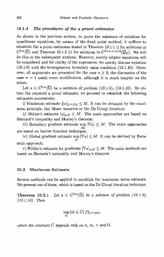
282 Elliptic and Parabolic Equations
10.1.4 The procedures of the a priori estimates
As shown in the previous section, to prove the existence of solutions for quasilinear equations, by means of the fixed point method, it suffices to establish the a priori estimates stated in Theorem 10.1.1 i) for solutions in C2'a{U) and Theorem 10.1.2 ii) for solutions in C2+a>1+a/2(QT). We will do this in the subsequent sections. However, merely elliptic equations will be considered and for clarity of the expression, we merely discuss equation (10.1.9) with the homogeneous boundary value condition (10.1.10). Moreover, all arguments are presented for the case n > 2; the discussion of the case n = 1 needs some modification, although it is much simpler on the whole.
Let u e C2'a(Ti) be a solution of problem (10.1.9), (10.1.10). To obtain the required a priori estimate, we proceed to establish the following estimates successively.
i) Maximum estimate ||«||L°°(n) < M. It can be obtained by the maximum principle, the Moser iteration or the De Giorgi iteration;
ii) Holder's estimate [w]a;n < M. The main approaches are based on Harnack's inequality and Morrey's theorem;
iii) Boundary gradient estimate sup|Vu| < M. The main approaches an
are based on barrier function technique; iv) Global gradient estimate sup |Vu| < M. It can be derived by Bern-
n stein approach;
v) Holder's estimate for gradients [Vu]a;n < M. The main methods are based on Harnack's inequality and Morrey's theorem.
10.2 Maximum Estimate
Several methods can be applied to establish the maximum norm estimate. We present one of them, which is based on the De Giorgi iteration technique.
Theorem 10.2.1 Let u € C2<a(ti) be a solution of problem (10.1.9), (10.1.10). Then
sup|u| < C||/||L°°(fi), n
where the constant C depends only on n, m, j and fi.
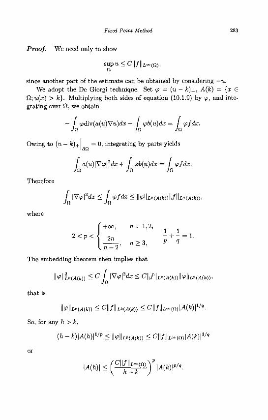
Fixed Point Method 283
Proof. We need only to show
suptt < C||/||LOo(n), n
since another part of the estimate can be obtained by considering — u. We adopt the De Giorgi technique. Set ip = (u — k)+, A(k) = {x e
Q;u(x) > k}. Multiplying both sides of equation (10.1.9) by <p, and integrating over CI, we obtain
— / <pdiv(a(u)'Vu)dx + / ipb(u)dx = / <pfdx. Ju Jn Jo.
Owing to (u — k)+ = 0, integrating by parts yields
/ a(u)\V<p\2dx + / (pb(u)dx = / ipfdx. Jet JQ Ja
Therefore
/ \Vip\2dx< / <pfdx<\\ip\\LP{A{k))\\f\\LHA{k)), Jn Jo.
where
+00, n = 1,2
2 < p < <
. n - 2
The embedding theorem then implies that
1 1
, n > 3 , P « 2n - + - = 1.
M\lp(A(k)) <C \^9?dx < C\\f\\L,iAik))\\(p\\Lp{Aik)), J it
that is
\\<P\\L*{AW) < C||/|U.(A(fc)) < C\\f\\L^n)\A(k)\^.
So, for any h> k,
(h - k)\A(h)\^ < y\\LP{A{k)) < C\\f\\Laola)\A(k)\^
or
\A(h)\<(CU^{Q)Y\A(k)\^.
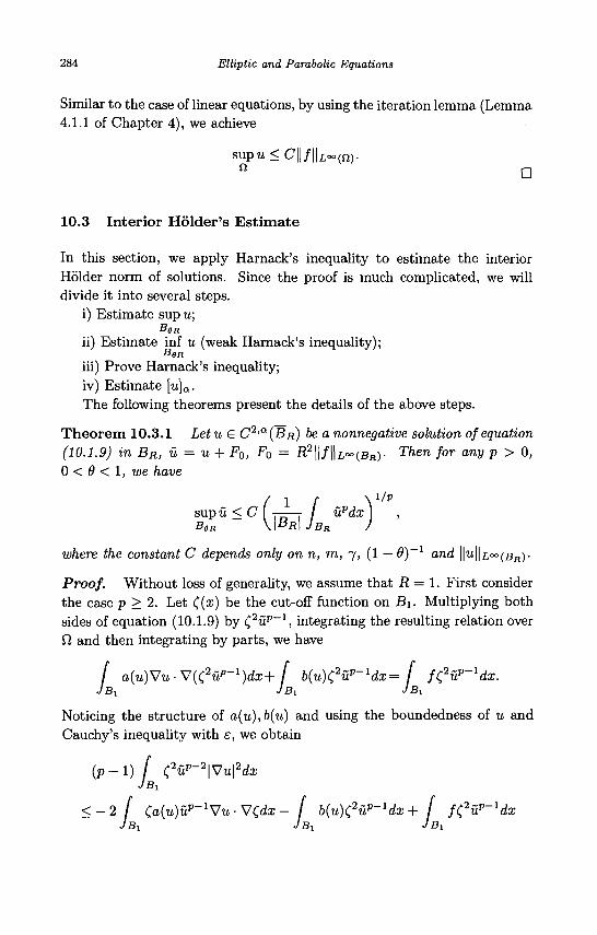
284 Elliptic and Parabolic Equations
Similar to the case of linear equations, by using the iteration lemma (Lemma 4.1.1 of Chapter 4), we achieve
S U p U < C | | / | | L ~ ( n ) .
10.3 Interior Holder's Estimate
In this section, we apply Harnack's inequality to estimate the interior Holder norm of solutions. Since the proof is much complicated, we will divide it into several steps.
i) Estimate supu; BeR
ii) Estimate inf u (weak Harnack's inequality); BeR
iii) Prove Harnack's inequality; iv) Estimate [u]a. The following theorems present the details of the above steps.
Theorem 10.3.1 Letu S C2,"(!?#) be a nonnegative solution of equation (10.1.9) in BR, u = u + F0, F0 = i?2 | | / | |L~ ( B f l ) . Then for any p > 0, 0 < 9 < 1, we have
sup u < C ( / updx ) , BeR \\BR\JBR J
where the constant C depends only on n, m, j , (1 — 9)~l and ||U||X,°°(BR)-
Proof. Without loss of generality, we assume that R=l. First consider the case p > 2. Let £(x) be the cut-off function on B\. Multiplying both sides of equation (10.1.9) by C2wp_1, integrating the resulting relation over fi and then integrating by parts, we have
/ a(u)Vu-V{<;2up-1)dx+ [ b(u)t2up-1dx= [ f(?up~ldx. JBi JBi JBi
Noticing the structure of a(u),b(u) and using the boundedness of u and Cauchy's inequality with e, we obtain
( p - 1 ) / C2up-2\Vu\2dx
<-2 [ C,a{u)up-1Vu-VC,dx- f b(u)(2up-1dx+ [ f<?up-ldx JB! JBi JBi
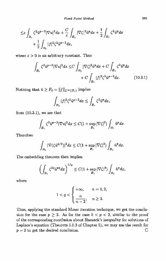
Fixed Point Method 285
<£ / <;2up-2\Vu\2dx + - f |VC|2updx + i / <?v?dx
+ U \f\2<2n"-2dx,
where e > 0 is an arbitrary constant. Thus
/ (2up-2\Vu\2dx<C [ \V<;\2updx + C [ (?updx JBi JB! JBi
+ C [ \f\2C2up-2dx. (10.3.1) JBi
Noticing that u > F0 = H/HLO^BJ) implies
/ \f\2<;2up-2dx < f C2updx, JBi JBx
from (10.3.1), we see that
/ <:2up~2\Vu\2dx < C(l + sup |VC|2) / updx. JBi Bi JBi
Therefore
/ |V(Cup / 2) |2da;<C(l + sup|VC|2) / updx. JBX S i JBX
The embedding theorem then implies
1/9
where
( f C2"upqdx) < C(l + sup|V<|2) / updx, \JBI ) Bi JB!
+oo, n = 1,2,
Kq<{ n
n-2 , n > 3.
Thus, applying the standard Moser iteration technique, we get the conclusion for the case p > 2. As for the case 0 < p < 2, similar to the proof of the corresponding conclusion about Harnack's inequality for solutions of Laplace's equation (Theorem 5.1.3 of Chapter 5), we may use the result for p — 2 to get the desired conclusion. •
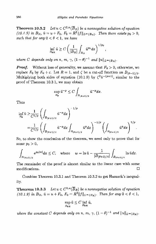
286 Elliptic and Parabolic Equations
Theorem 10.3.2 Letu G C 2 , Q ! ( B R ) be a nonnegative solution of equation (10.1.9) in BR, u = u + F0, FQ = R2\\f\\L°°(BR)- Then there exists p0 > 0, such that for any 0 < 0 < 1, we have
kL<"*)' \ l / P O
inf u > C ,' . _, BeR \ \Bf
where C depends only on n, m, 7, (1—9) and ||U||£,OO(BB).
Proof. Without loss of generality, we assume that Fo > 0, otherwise, we replace Fo by F0 + e. Let R = 1, and ( b e a cut-off function on B(0+iy2-Multiplying both sides of equation (10.1.9) by £2u~(p+1\ similar to the proof of Theorem 10.3.1, we may obtain
sup u~p<C J u-pdx. Be * 'B(e+i) /2
Thus
- 1 / p
inf u > „ . I / u vdx Be -CVp\JBlt+1„ MX *"
\JB(e+i)/2
™[L *~PdxL H [L W £>(S + l) /2 •/-£>(e + l) /2 / V - 0 ( 0 + 1
1/p / n \ 1/p
updx ) . CM
\ J D(.e+i)/2 J •D(e+i)/2 / \ J D(e+i)/2
So, to show the conclusion of the theorem, we need only to prove that for some po > 0,
/ ePo^dx < C, where w = lnu - — - / \nudx. JB(o+i)/2 | - B ( 9 + 3 ) / 4 | JB(e+3)/4
The remainder of the proof is almost similar to the linear case with some modifications. •
Combine Theorem 10.3.1 and Theorem 10.3.2 to get Harnack's inequality.
Theorem 10.3.3 Letu G C2,C"(BR) be a nonnegative solution of equation (10.1.9) in BR, u = u + F0, F0 = R?\\f\\L°°(BR)- Then for any 0 < 0 < 1,
sup u < C inf u, BeR
BsR
where the constant C depends only on n, m, 7, (1 — 6)~l and ||U||Z,°°(BB)-
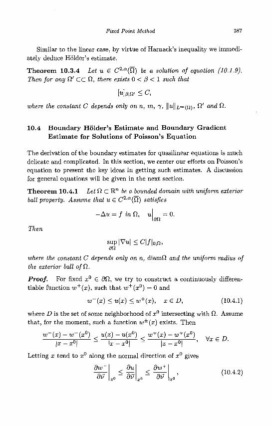
Fixed Point Method 287
Similar to the linear case, by virtue of Harnack's inequality we immediately deduce Holder's estimate.
Theorem 10.3.4 Let u € C2,a(fi) be a solution of equation (10.1.9). Then for any Cl' CC f2, there exists 0 < 0 < 1 such that
[u]p;n- < C,
where the constant C depends only on n, m, 7, ||w||z,°°(n), H' and Q.
10.4 Boundary Holder's Estimate and Boundary Gradient Estimate for Solutions of Poisson's Equation
The derivation of the boundary estimates for quasilinear equations is much delicate and complicated. In this section, we center our efforts on Poisson's equation to present the key ideas in getting such estimates. A discussion for general equations will be given in the next section.
Theorem 10.4.1 Let 0. C M" be a bounded domain with uniform exterior ball property. Assume that u S C2'a(Q) satisfies
—Au = / in Q,,
Then
= 0. an
s u p | V u | < C | / | o ; n , an
where the constant C depends only on n, diamf2 and the uniform radius of the exterior ball ofQ.
Proof. For fixed a;0 € <9fi, we try to construct a continuously differen-tiable function w^(x), such that w±(x°) = 0 and
w~(x) <u(x) <w+(x), xeD, (10.4.1)
where D is the set of some neighborhood of x° intersecting with fi. Assume that, for the moment, such a function w±(x) exists. Then
w~(x) — w~(x°) u(x) — u(x°) w+(x) — w+(x°)
Letting x tend to z° along the normal direction of x° gives
dw~
dV du dw+
0u (10.4.2)
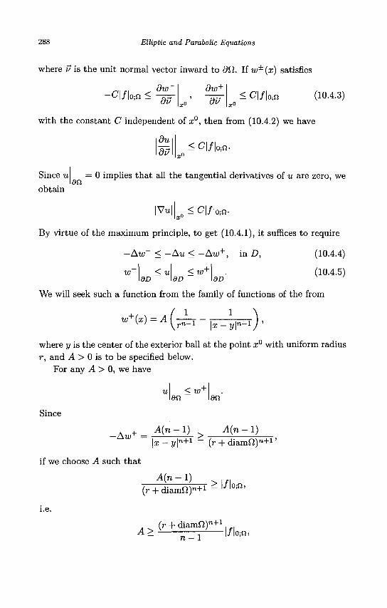
288 Elliptic and Parabolic Equations
where u is the unit normal vector inward to <90. If w±(x) satisfies
-Cl/loiO < dw
dV
dw+
p 0 ' dv < C|/ |0 in (10.4.3)
with the constant C independent of x°, then from (10.4.2) we have
< C|/ |0 ;n. du
Since u
obtain dn
0 implies that all the tangential derivatives of u are zero, we
|Vu| < C | / | 0 i n .
By virtue of the maximum principle, to get (10.4.1), it suffices to require
- A w " < -Au < - A w + , in D, (10.4.4)
w 8D
<U <W+
dD dD (10.4.5)
We will seek such a function from the family of functions of the from
1 W+(x) = A ( r - •: ; r |
where y is the center of the exterior ball at the point a;0 with uniform radius r, and A > 0 is to be specified below.
For any A > 0, we have
u\ < w+
\an an
Since
-Au^.^.U A{n'l) \x-y\n+l ~ (r + d i amn) n + 1 '
if we choose A such that
A{n-l) ^ I J . I
(r + d iamf t )^ 1 " l 7 | 0 ; " '
(r + d i a m ^ ) ^ 1
A> — | / |0 in,
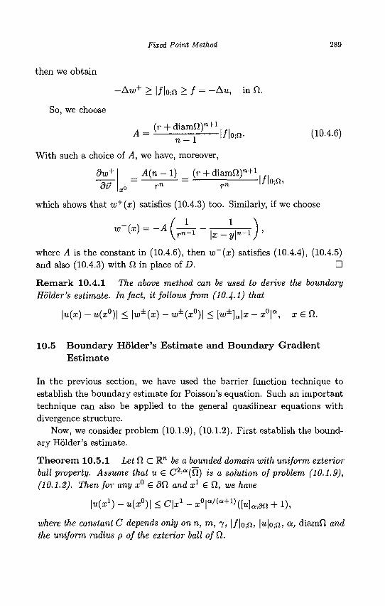
Fixed Point Method 289
then we obtain
-Aw+ > | / |0 in > / = - A « , in SI.
So, we choose
(r + diamfi)"+1
n - 1
With such a choice of A, we have, moreover,
dw+
I/loin- (10-4.6)
9?
A(n - 1) (r + d iamn)" + 1 . ,. ~~ — | / | o ; n , ir* it fit
which shows that w+(x) satisfies (10.4.3) too. Similarly, if we choose
1 1 ~(x) — ** , , , , ,
*• I \j.n-\ | x _ ^ | n - l
where A is the constant in (10.4.6), then w~(x) satisfies (10.4.4), (10.4.5) and also (10.4.3) with CI in place of D. D
Remark 10.4.1 The above method can be used to derive the boundary Holder's estimate. In fact, it follows from (10.4-1) that
\u(x) - u(x°)\ < lur^x) - w±(x°)\ < [ u r ^ l x - x°\a, x e SI.
10.5 Boundary Holder's Estimate and Boundary Gradient Estimate
In the previous section, we have used the barrier function technique to establish the boundary estimate for Poisson's equation. Such an important technique can also be applied to the general quasilinear equations with divergence structure.
Now, we consider problem (10.1.9), (10.1.2). First establish the boundary Holder's estimate.
Theorem 10.5.1 Let SI C Rn be a bounded domain with uniform exterior ball property. Assume that u £ C2'a(Sl) is a solution of problem (10.1.9), (10.1.2). Then for any x° € dSl and x1 £ SI, we have
K x 1 ) - u(x°)\ < Qx1 - x T / ( a + 1 ) ( M a ; a n + 1),
where the constantC depends only onn, m, 7, |/|o;fi) Mo;n, a> diamfi and the uniform radius p of the exterior ball of SI.
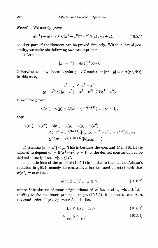
290 Elliptic and Parabolic Equations
Proof. We merely prove
uix1) - u(x°) < Qx1 - z°p /(a+1)(M<*;9fi + 1); (10-5.1)
another part of the theorem can be proved similarly. Without loss of generality, we make the following two assumptions:
i) Assume
l a ; 1 -^ 0 ! =dist(x1 ,dft) .
Otherwise, we may choose a point y £ dD, such that \xl —y\= dist(x1, dfl). In this case,
.1 y \ < l x l ™0, \x — y\ S \x — x \ ,
y.0\ \y -x°\<\y-x1\ + Ix1 - a;01 < 21a:1
If we have proved
^a;1) - u(y) < C\xx - y\a^a+l)([u]a]9Q + 1),
then
u(x*) — u(a;°) =u(x1) — u(y) + u(y) — u(a;0)
<C\xx - y|a / ( Q + 1 )([«]a i8n + 1) + C\y - x°\a[u}am
<C\x1-x°\aKa+1'>([u]a.,9n + l).
ii) Assume \xl — x°\ < p. This is because the constant C in (10.5.1) is allowed to depend on p, if Ix1 — a;°| > p, then the desired conclusion can be derived directly from |u|o;n < C.
The basic idea of the proof of (10.5.1) is similar to the one for Poisson's equation in §10.4, namely, to construct a barrier function w(x) such that w(x°) = u(x°) and
u(x) < w{x), xeD, (10.5.2)
where D is the set of some neighborhood of a;0 intersecting with Cl. According to the maximum principle, to get (10.5.2), it suffices to construct a second order elliptic operator L such that
Lu < Lw, in D, (10.5.3)
u < w dD
(10.5.4) dD
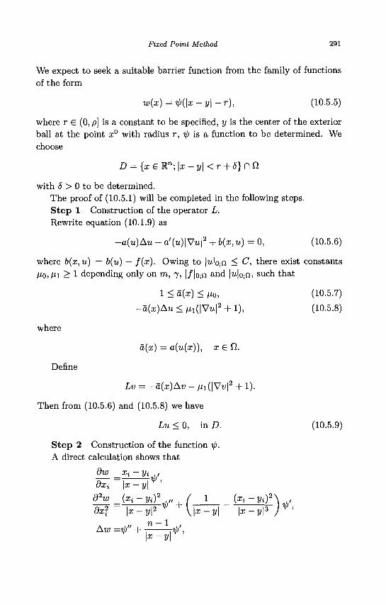
Fixed Point Method 291
We expect to seek a suitable barrier function from the family of functions of the form
w(x) = tp(\x — y\ — r) , (10.5.5)
where r € (0, p] is a constant to be specified, y is the center of the exterior ball at the point x° with radius r, tp is a function to be determined. We choose
D = {x £ Kn; \x - y\ < r + 6} n fi
with 5 > 0 to be determined. The proof of (10.5.1) will be completed in the following steps. S tep 1 Construction of the operator L. Rewrite equation (10.1.9) as
-o(u)Au - a'(u)|Vu|2 + b(x, u) = 0, (10.5.6)
where b(x,u) = b(u) — f(x). Owing to |u|o;n < C, there exist constants Mo, Mi > 1 depending only on m, 7, |/|o ;n and |u|o-,n, such that
1 < a(x) < fio, (10.5.7)
-a(x)Au < /xi(|Vu|2 + 1), (10.5.8)
where
a(x) = a(u(x)), x e fi.
Define
Lv = - 5 ( X ) A D - m(\Vv\2 + 1).
Then from (10.5.6) and (10.5.8) we have
Lu < 0, in D. (10.5.9)
S tep 2 Construction of the function tp. A direct calculation shows that
dw_ _Xj-yj ,
dxi \x — y\
d2w _ (xi - Vi)2,,, ( 1 _ (xj-yi)2\ , dx2 \x-y\2 \\x-y\ \x - y\3
. ,,, n — 1 ,, AW =1p" + rip',
\x-y\
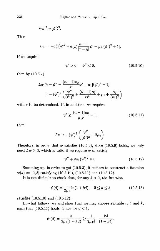
292 Elliptic and Parabolic Equations
\Vw\2 =(ip')2-
Thus
Lw = -a(x)V" - a(x)^——tf - ^[{ip')2 + 1].
If we require
ip' > 0, V" < 0, (10.5.10)
then by (10.5.7)
Lw > _ ^ _ ("-^)/*y _ m[(v / )2 + x]
= -(^)2f74 + l !^ £+m+ Ml V(V>')2 r-V-' ( V O 2
with r to be determined. If, in addition, we require
V / > ^ ^ + l, (10.5.11) Mir
then
Therefore, in order that w satisfies (10.5.3), since (10.5.9) holds, we only need Lw > 0, which is valid if we require tp to satisfy
ip" + 2li1(ip')2 < 0 . (10.5.12)
Summing up, in order to get (10.5.3), it suffices to construct a function ip(d) on [0,5] satisfying (10.5.10), (10.5.11) and (10.5.12).
It is not difficult to check that, for any k > 0, the function
V»(d) = ^ - l n ( l + Jfcd), 0<d<5 (10.5.13) 2/xi
satisfies (10.5.10) and (10.5.12). In what follows, we will show that we may choose suitable r, 5 and k,
such that (10.5.11) holds. Since for d < 5,
, / / « k * kS
2fj,i(l + kd) ~ 2fiiS (1 + kS)'
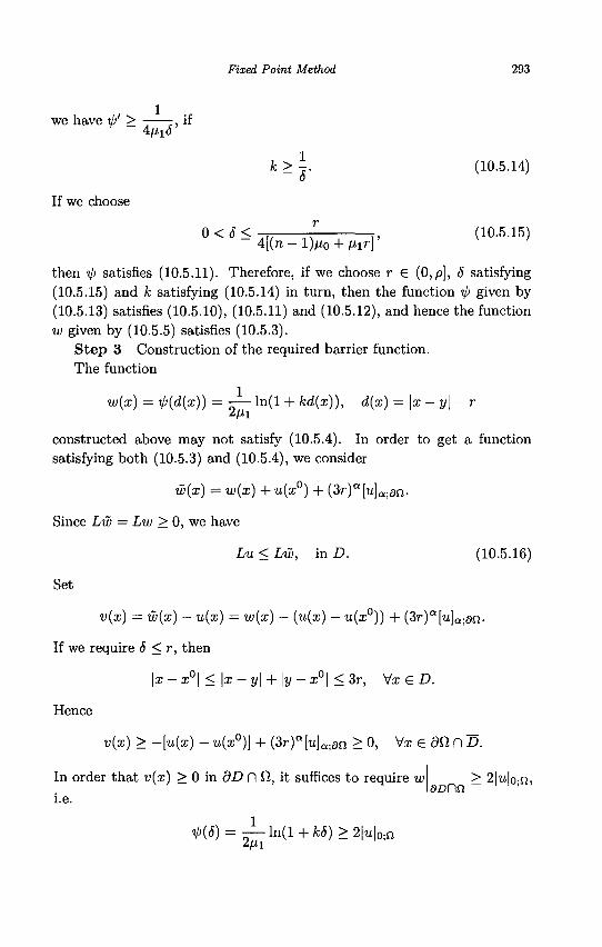
Fixed Point Method 293
we have ib' > -, if 4/Xi<5
If we choose
k>\. (10.5.14) o
0 < 5^ 777 TT"^ : v (10.5.15) 4[(n - l)/x0 + Hir]
then xp satisfies (10.5.11). Therefore, if we choose r e {0,p}, 5 satisfying (10.5.15) and k satisfying (10.5.14) in turn, then the function V given by (10.5.13) satisfies (10.5.10), (10.5.11) and (10.5.12), and hence the function w given by (10.5.5) satisfies (10.5.3).
Step 3 Construction of the required barrier function. The function
w(x) = ip(d(x)) = -— ln(l + kd(x)), d(x) = \x — y\ — r 2/xi
constructed above may not satisfy (10.5.4). In order to get a function satisfying both (10.5.3) and (10.5.4), we consider
w(x) = w(x) + u(x°) + (3r)a[u]a ;an .
Since Lw — Lw > 0, we have
Lu < Lw, in D. (10.5.16)
Set
v(x) = w(x) - u(x) = w(x) - (u(x) - u(x0)) + (3r)a\u]a.dn.
If we require 5 < r, then
\x-x°\ < \x-y\ + \y-x°\ < 3r, Mx&D.
Hence
v{x) > -\u{x) - u{x0)] + (3r)a[u]a;dn > 0, Vz G OQ D D.
In order that v(x) > 0 in 3D n Vt, it suffices to require w ^ > 2|u|o;n,
i.e.
4>(5) = ^-ln(l + k5)>2\u\0.n
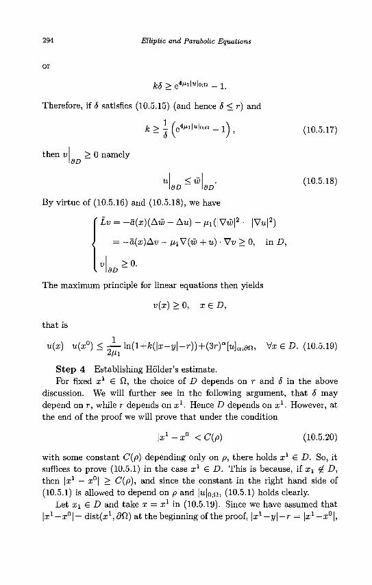
294 Elliptic and Parabolic Equations
or
Therefore, if S satisfies (10.5.15) (and hence 5 < r) and
fc>i(e4"l|ul°'n-lV
then v dD
> 0 namely
dD < W
dD
(10.5.17)
(10.5.18)
dD
By virtue of (10.5.16) and (10.5.18), we have
' Lv = -a(x)(Aw - Au) - /xi(|Vw|2 - |Vu|2)
-a(x)Av - fn\7(w + u)-Vv>0, in D,
> 0 .
The maximum principle for linear equations then yields
v(x) > 0, x £ D,
that is
u(x)-u(x°) < J - ln(l+k(\x-y\-r)) + {3r)a[u)a,dn, Vz € £>. (10.5.19)
Step 4 Establishing Holder's estimate. For fixed x1 € fi, the choice of D depends on r and 5 in the above
discussion. We will further see in the following argument, that 5 may depend on r, while r depends on xl. Hence D depends on x1. However, at the end of the proof we will prove that under the condition
la;1-a;0] < C(p) (10.5.20)
with some constant C(p) depending only on p, there holds x1 € D. So, it suffices to prove (10.5.1) in the case x1 £ D. This is because, if xi £ D, then la;1 — a;°| > C(p), and since the constant in the right hand side of (10.5.1) is allowed to depend on p and |u|o;n, (10.5.1) holds clearly.
Let xi £ D and take x = x1 in (10.5.19). Since we have assumed that jx1— a:°|= dist(a;1,9n) at the beginning of the proof, \x1—y\—r = ja;1—x°|,
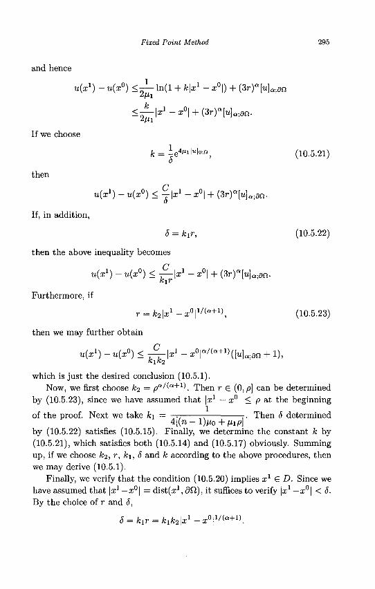
Fixed Point Method 295
and hence
uOc1) - u(x°) < J - m(l + fcla;1 - x°|) + (3r)a[u}a.,an
If we choose
then
< ^ - | a ; 1 - x 0 | + (3r) o [«] a ; e n .
jb = L4/nMo i n j (10.5.21) o
uix1) - u{x°) <^\xx- x°\ + (3r)a{u]a,an. d
If, in addition,
6 = kir, (10.5.22)
then the above inequality becomes
uix1) - u(x°) < -^{x1 - x°\ + (3 r )>] Q ; an .
Furthermore, if
r = k2\xl -x°\l/{a+1\ (10.5.23)
then we may further obtain
uix1) - u(x°) K-^-lx1- x°\a^a+1\[u}a.tdn + 1), K1K2
which is just the desired conclusion (10.5.1). Now, we first choose k<i = pa/(a+1\ Then r e (0,p] can be determined
by (10.5.23), since we have assumed that la;1 — x°\ < p at the beginning
of the proof. Next we take k\ = -7- -. Then 5 determined 4[(n - l)fi0 + fiip\
by (10.5.22) satisfies (10.5.15). Finally, we determine the constant k by (10.5.21), which satisfies both (10.5.14) and (10.5.17) obviously. Summing up, if we choose k2, r, k\, S and k according to the above procedures, then we may derive (10.5.1).
Finally, we verify that the condition (10.5.20) implies x1 S D. Since we have assumed that la;1 —a;°| = dist(a;1, d£l), it suffices to verify \xx — x°\ < 6. By the choice of r and 6,
<S = jfc1r = Jfe1fc2|a:1-a:0|1/(o","1)-
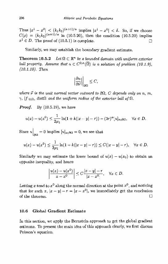
296 Elliptic and Parabolic Equations
Thus la;1 - x°| < (fcifc2)(a+1)/a implies la;1 - a;°| < S. So, if we choose C(p) = (k1k2)
(a+1)/a in (10.5.20), then the condition (10.5.20) implies x1 € D. The proof of (10.5.1) is complete. •
Similarly, we may establish the boundary gradient estimate.
Theorem 10.5.2 Let D, c R™ be a bounded domain with uniform exterior ball property. Assume that u £ C2>a(Q,) is a solution of problem (10.1.9), (10.1.10). Then
du <C,
an
where v is the unit normal vector outward to dQ,, C depends only on n, m, 7) |/|o;fi, distfi and the uniform radius of the exterior ball of CI.
Proof. By (10.5.19), we have
u(x) - u(x°) < - ! - ln(l + k(\x -y\- r)) + (3r)a[u]a;an, Vx € D.
Since u an
= 0 implies [w^an = 0, we see that
u(a;) - u(x°) < -— ln(l + k(\x -y\- r)) < C(\x -y\- r), Va; G D. 2/Xi
Similarly we may estimate the lower bound of u{x) — u(xo) to obtain an opposite inequality, and hence
u{x) — u(x°) <C \x-y\
\x — x 01 ' V x e D .
Letting x tend to x° along the normal direction at the point x°, and noticing that for such x, \x — y\ — r = \x — x°\, we immediately get the conclusion of the theorem. •
10.6 Global Gradient Estimate
In this section, we apply the Bernstein approach to get the global gradient estimate. To present the main idea of this approach clearly, we first discuss Poisson's equation.
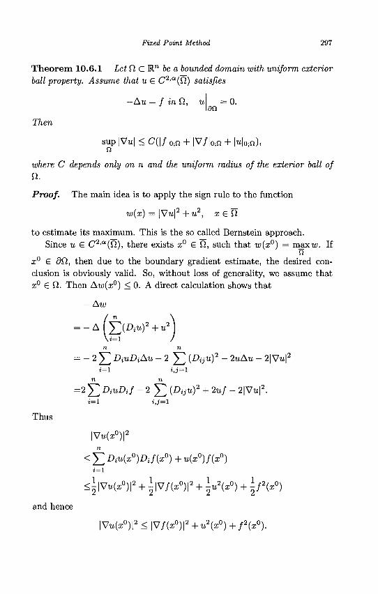
Fixed Point Method 297
Theorem 10.6.1 Let fi C Rn be a bounded domain with uniform exterior ball property. Assume that u G C2'a(Q) satisfies
—Au = f inQ, u
Then
= 0. an
sup |V«| < C( | / |0 ;n + |V/ |0 in + |u|0;n), n
where C depends only on n and the uniform radius of the exterior ball of
n. Proof. The main idea is to apply the sign rule to the function
w(x) = | V u | 2 + u 2 , x e f i
to estimate its maximum. This is the so called Bernstein approach. Since u G C2 ,a(fi), there exists x° G Q, such that w(x°) = maxra. If
n x° G dSl, then due to the boundary gradient estimate, the desired conclusion is obviously valid. So, without loss of generality, we assume that x° G fi. Then Aw(x°) < 0. A direct calculation shows that
-Aw
= -A(J2(Diu)2+uA n n
= - 2 2 DiuDiAu -2^2 (Diju)2 ~ 2uAu - 2|Vu|2
n n
=2 Y, DiuDif -2^2 (Dijuf + 2uf - 2|Vu|2.
Thus
|Vu(z°)|2
n
< ^2 Diu(x0)Dif(x0) + u(x°)f(x°) t = i
<J|VM(x°) | 2 + i | V / ( z ° ) | 2 + \u\x°) + \f\x°)
and hence
\Vu(x°)\2 < |V/(z°) | 2 + u2(x°) + f2(x°).
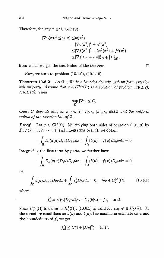
298 Elliptic and Parabolic Equations
Therefore, for any x G Q, we have
|Vu(:r)|2 <w(x) <w(x°)
=\Vu(x°)\2+u2(x°)
<\Vf(x°)\2 + 2u2(x°)+f2(x0)
<|V/|g.n + 2Hg.n + |/|g.n,
from which we get the conclusion of the theorem. •
Now, we turn to problem (10.1.9), (10.1.10).
Theorem 10.6.2 Let Cl c l ™ be a bounded domain with uniform exterior ball property. Assume that u € C2'a(Q.) is a solution of problem (10.1.9), (10.1.10). Then
sup|Vu| < C,
where C depends only on n, m, 7, |/|o ;n, |w|Q;n, distfi and the uniform radius of the exterior ball o/fi.
Proof. Let <p G Co°(fi). Multiplying both sides of equation (10.1.9) by Dk(p (k = 1,2, • • • , n), and integrating over fi, we obtain
- / Di(a(u)Diu)Dk<pdx + f (b(u) - f(x))Dkipdx = 0. Jn Jn
Integrating the first term by parts, we further have
- [ Dk(a(u)DiU)Diipdx + f (b(u) - f{x))Dk<pdx = 0, Jn Jn
i.e.
/ a{u)DikuDnpdx + [ f^D^dx = 0, Vy> G C£°(fi), (10.6.1) Jn Jn
where
fl = a'(u)DkuDiU - 5ik(b(u) - / ) , in ft.
Since C$°(Q.) is dense in H&(Q), (10.6.1) is valid for any (p G H^(Cl). By the structure conditions on a(u) and b(u), the maximum estimate on u and the boundedness of / , we get
\fl\<C(l + \Du\2), in ft.
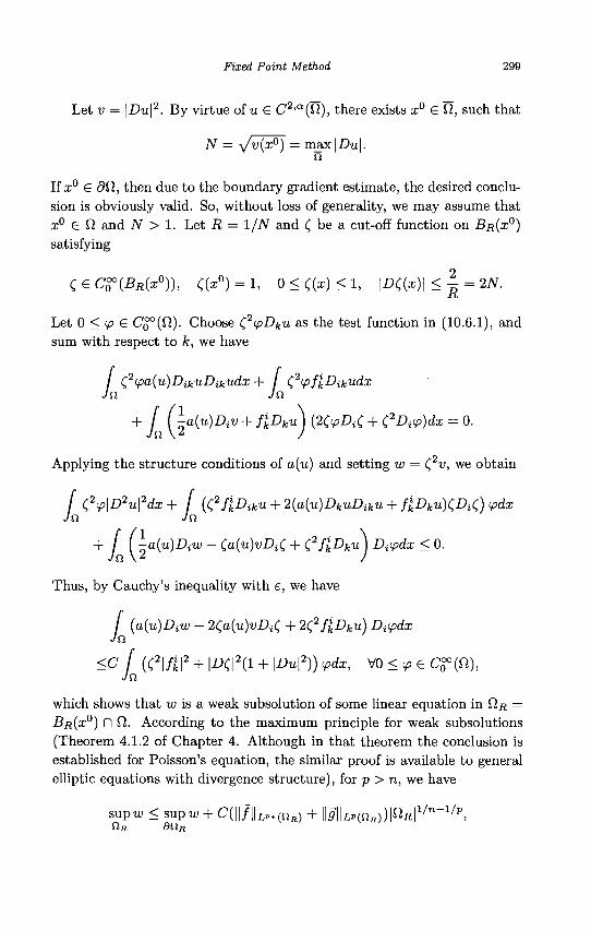
Fixed Point Method 299
Let v = |Du|2. By virtue of u e C2'a{Vt), there exists x° € fi, such that
N = y/v(x°) = max|Dw|.
If a;0 G dil, then due to the boundary gradient estimate, the desired conclusion is obviously valid. So, without loss of generality, we may assume that i ° e f i and N > 1. Let R = I/TV and £ be a cut-off function on BR(x°) satisfying
<;eCZ°(BR(x0)), C(x°) = l, 0 < C ( z ) < l , |Z>C(z)l < I = 2JV.
Let 0 < i p £ Co°(fi). Choose Q2ipDku as the test function in (10.6.1), and sum with respect to k, we have
/ (2(pa(u)DikuDikudx + / C,2(pfkDikudx Jn Jn
+ J (^a{u)DiV + flkDku^j ( 2 C P A C + C2D^)dx = 0.
Applying the structure conditions of a(u) and setting w = (2v, we obtain
/ £2<p\D2u\2dx + f {C?PkDiku + 2{a(u)DkuDiku + /JDfcu)CAC) V>dx Jn Jo,
+ f (±a(u)DiW - (a{u)vDi<; + (2flDku) DiVdx < 0.
Thus, by Cauchy's inequality with e, we have
/ (a(u)DiW - 2Ca(u)vDiC + 2C?PkDku) Dupdx
<C [ (e\fk\2 + |£>C|2(1 + \Du\2)) ipdx, V0 < ^ e C0°°(ft),
Jo
which shows that w is a weak subsolution of some linear equation in flu = BR(X°) n fl. According to the maximum principle for weak subsolutions (Theorem 4.1.2 of Chapter 4. Although in that theorem the conclusion is established for Poisson's equation, the similar proof is available to general elliptic equations with divergence structure), for p > n, we have
supu; < suPw + C(\\f\\LP.{nR) + \\ghHoR))\fln\1/n-1/p, OR dOR
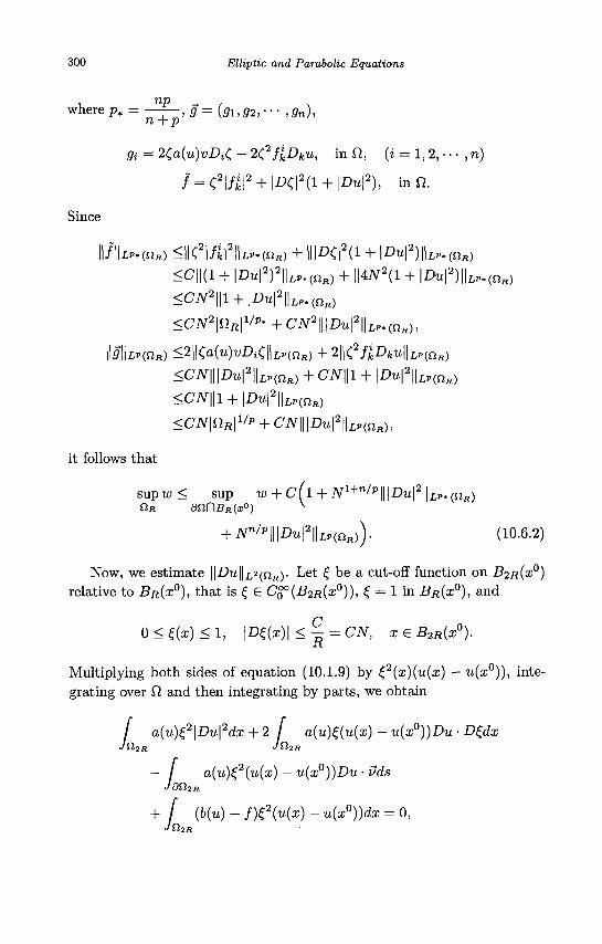
300 Elliptic and Parabolic Equations
where p» = — — , g = {gi,g2,--- ,9n), Tl ~f~ P
9i = 2Co(u)i;AC " 2C2fkDku, in O, (i = 1,2, • • • , n)
/ = C 2 | / j | 2 + |£>C|2(l + U?u|2), in O.
Since
ll/llL-(nH)<llC2|/il2IUp.(njl) + |||I>C|2(l + l^|a)llL-.(nH) <C||(1 + \Du\2)2\\LP,(nR) + IKiV2(l + |D«| a) | |Lp. ( n j l )
<CN2\\1 + | JD t t |2 | |LP , ( n a )
<C^ 2 | n f l | 1 / p -+C^ 2 | | | £>u | 2 |Up . ( n j l ) ,
HflIlLp(n„) <2Ua(u)vDiC\\LHnR)+2\\eflDku\\L^R)
<CN\\\Du\2\\LP{nR) + CN\\1 + |Z*i|2|Up(njl)
<CN\\l + \Du\2\\LHnR)
<CN\nR\VP + CN\\\Du\2\\LP{nR),
it follows that
s u p w < sup w + c(l + N1+n/p\\\Du\2\\LP.{nR) ft* dnr\BR(x°) v
+ Nn/p\\\Du\2\\LHaR)). (10.6.2)
Now, we estimate ||Du||i2(fjR). Let £ be a cut-off function on B2R(X°) relative to BR(x°), that is £ G C§°(B2ie(a;0)), £ = 1 in Bfi(x°), and
0 < £(z) < 1, |£>£(z)| < ^ = C7V, l £ B2fl(cc0).
Multiplying both sides of equation (10.1.9) by (,2(x)(u(x) - u(x0)), integrating over fi and then integrating by parts, we obtain
/ a(u)Z2\Du\2dx + 2 I a(u)£(u(x) - u(x°))Du • D£dx
- J a(u)£2(u(x) - u{x°))Du • vds JdQ2R
+ f (b(u) - f)Z2{u(x) - u{x°))dx = 0, J Hop
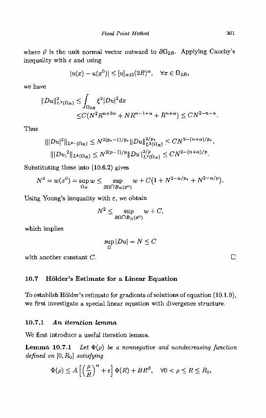
Fixed Point Method 301
where v is the unit normal vector outward to 8Q.2R- Applying Cauchy's inequality with e and using
|«(x) - u(x°)| < [u]a.n(2R)a, Vx e Q2R,
l ^ l l ^ ( n „ ) < / $2\Du\2dx
we have
; / e\Duf JQ2R,
<C{N2Rn+2a + NRn~1+a + Rn+a) < CN2-n-a.
Thus
\\\Du\2\\L,.(na) < N2^-W*\\DU\\%^R) < C i V 2 - ( " + ^ %
IH^|2 |UP (nK) < N>W\\Du\\%>(nit) < C i V 2 - ( " + ^ .
Substituting these into (10.6.2) gives
N2 = w(x°) = sup w < sup w + C{\ + N2~a/P' + JV2-Q/p). nR anr\BR(x°)
Using Young's inequality with e, we obtain
N2 < sup w + C, dClf)BR(x°)
which implies
sup \Du\ =N <C n
with another constant C. O
10.7 Holder's Estimate for a Linear Equation
To establish Holder's estimate for gradients of solutions of equation (10.1.9), we first investigate a special linear equation with divergence structure.
10.7.1 An iteration lemma
We first introduce a useful iteration lemma.
Lemma 10.7.1 Let <3>(p) be a nonnegative and nondecreasing function defined on [0, RQ] satisfying
$(p) < A [ ( - 0 " + e] $(fl) + BR13, \/0<p<R<Ro,
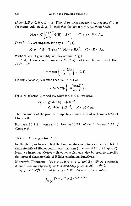
302 Elliptic and Parabolic Equations
where A, B > 0, 0 < j3 < a. Then there exist constants £0 > 0 and C > 0 depending only on A, a, (3, such that for any 0 < e < £o, there holds
*(/o) < C V0 < p < R < RQ.
Proof. By assumption, for any r £ (0,1),
$(TR) < Ara{l + eT~a)$(R) + BR13, \/0<R< R0.
Without loss of generality we may assume A > 1. First, choose a real number v £ (/?, a) and then choose r such that
2ArQ = TV or
— {-^}c(M,. Finally, choose £o > 0 such that £oT_a < 1 or
f ln(2A) I 0 < £0 < exp - - a — i \ .
\ a-v J
For such selected v, r and £Q, when 0 < e < £o, we have
<p(rR) <2ATa^(R)+BRf}
<TV$(R) + BR0, V0<R< R0.
The remainder of the proof is completely similar to that of Lemma 6.2.1 of Chapter 6. •
Remark 10.7.1 When e = 0, Lemma 10.7.1 reduces to Lemma 6.2.1 of Chapter 6.
10.7.2 Morrey's theorem
In Chapter 6, we have applied the Campanato spaces to describe the integral characteristic of Holder continuous functions (Theorem 6.1.1 of Chapter 6). Now, we introduce Morrey's theorem, which can also be used to describe the integral characteristic of Holder continuous functions.
Morrey's Theorem Let p > 1, 0 < a < 1, and Q C Rn be a bounded domain with appropriately smooth boundary (such as dQ. € Cl>a).
i) Ifu€ W^(Rn) and for any i £ l " and p> 0, there holds
[ \\7u(y)\Pdy<Cpn-p+pa, JBp(x)
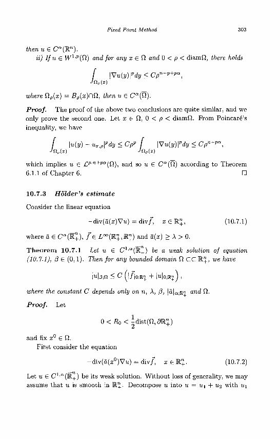
Fixed Point Method 303
thenueCa(Rn). ii) If u & W1,P(Q) and for any x G ft and 0 < p < diamft, there holds
f \Vu(y)\pdy<Cpn~p+pa,
where Qp{x) = Bp(x)C)Q, then u € CQ(ft).
Proof. The proof of the above two conclusions are quite similar, and we only prove the second one. Let x G ft, 0 < p < diamft. From Poincare's inequality, we have
f \u(y) - uxJpdy < Cpp f \Vu{y)\pdy < Cpn+pa,
Jn„(x) Jn„(x)
which implies u G Cp'n+pa(fl), and so u G CQ(ft) according to Theorem 6.1.1 of Chapter 6. •
10.7.3 Holder's estimate
Consider the linear equation
-div(5(i)Vu) = div/, i € l " + , (10.7.1)
where a G CQ(R+), /*G L°°(R^,Rn) and a{x) > A > 0.
Theorem 10.7.1 Let u G C1 , Q(R+) be a weak solution of equation (10.7.1), (3 G (0,1). Then for any bounded domain ft CC R™, we have
M/3;fi < C [\f\o-Ml + lu|0;K^J ,
where the constant C depends only on n, A, 0, |a|Q;R» and ft.
Proof. Let
0<Ro < idist(ft,<9R!^)
and fix x° G ft. First consider the equation
-div(a(z°)Vu) = div/, i £ l " + . (10.7.2)
Let u G C1 , Q(R+) be its weak solution. Without loss of generality, we may assume that u is smooth in R™. Decompose u into u = U\ + Ui with u\
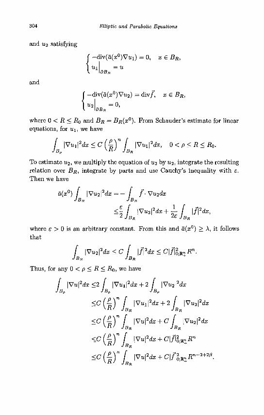
304 Elliptic and Parabolic Equations
and U2 satisfying
and
-div(a(x°)Vui) =0 , x £ BR,
Ul dBR
-div(a(x0)Vu2) = div/, x € BR,
U2 dBt
= 0,
where 0 < R < R0 and BR = BR(X°). Prom Schauder's estimate for linear equations, for u\, we have
/ \Wui\2dx <C(^-Y I |Vui|2rfa;, 0 < p < R < RQ. JB„ ^R> JBR
To estimate U2, we multiply the equation of U2 by U2, integrate the resulting relation over BR, integrate by parts and use Cauchy's inequality with e. Then we have
a(x°) J \Vu2\2dx = - J f-Vu2dx
J BR • ' B R
<£- [ \Vu2\2dx + ±[ \f\2dx,
1 JBR Z£ J BR
where s > 0 is an arbitrary constant. From this and d(x°) > X, it follows that
\Wu2\2dx < C [ \f\2dx < C\f\2
0.RnRn. JBR
Thus, for any 0 < p < R < Ro, we have
/ \Vu\2dx<2 [ \'Vu1\2dx + 2 [ \Wu2\
2dx JBP JB„ JBp
^ ( i Y f \Vu1\2dx + 2 f \Wu
y R J J BR JBR
<c(^)n f \Vu\2dx + C [ \Wu2\2dx yRJ JBR JBR
- C ( R Y J \Vu\2dx + C\f\2.RlRn
2\2dx
2+2/3
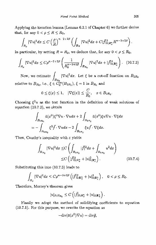
Fixed Point Method 305
Applying the iteration lemma (Lemma 6.2.1 of Chapter 6) we further derive that, for any 0 < p < R < RQ,
JB \Vu?dx<c(t)n~2+20(KJB \Vu\Hx + C\f\lMlRn-^
In particular, by setting R = RQ, we deduce that, for any 0 < p < RQ,
[ \S7u\2dx<Cpn-2+2l3(—^[ \Vu\2dx + \f%Rn). (10.7.3) JBP \R0
P JBRO +J
Now, we estimate / \S7u\2dx. Let £ be a cut-off function on B2R0 JBRO
relative to BRo, i.e., £ <E C0X{B2R0), £ = 1 in BRo and
0<t(x)<l, | V £ ( z ) | < £ , x€B2Ro.
Choosing £2it as the test function in the definition of weak solutions of equation (10.7.2), we obtain
J a(x°)£2Vu • Vudx + 2 I a{x°)£uVu • V£<£r •> B2R0 J BlRQ
= - J i2f- Vudx -2 f fit/- V£dx. J B2RQ J B2R0
Then, Cauchy's inequality with e yields
u IB2RO
2dx f \Wu\2dx <C ( f \f\2dx + J •'BRQ \ J B2RQ J B ;
<C (|/1§!R~ + |«|§iR») • (10.7.4)
Substituting this into (10.7.3) leads to
j \Vu\2dx<Cpn-2+2P(\ff0.n+\u\2.&n), 0<p<Ro.
Therefore, Morrey's theorem gives
[U]/3;BR0 < C [\f\o-Rl + Mo;R") .
Finally we adopt the method of solidifying coefficients to equation (10.7.1). For this purpose, we rewrite the equation as
—div(a(a;°)Vu) = divg,
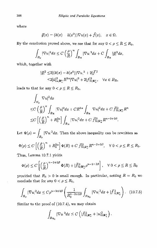
306 Elliptic and Parabolic Equations
where
g{x) = (a(x) - a(x°))Vu(x) + f(x), x e Q.
By the conclusion proved above, we see that for any 0 < p < R < RQ,
f \Vu\2dx < C (^Y J \Vu\2dx + C f \g\2dx, J B p •'•' J BR J BR
which, together with
\g\2<2\(a(x)-a(x°))Vu\2 + 2\f\2
<2[a]2.Rni?2a |Vu|2 + 2 | / ] 2; R ? , Vx G BR,
leads to that for any 0 < p < R < Ro,
\Vu\2dx
( 4 ) " / \Vu\2dx + CR2a [ \Wu\2dx + C\f\lRlRn
yRJ J BR J BR +
<C
.n-2+2/3
Let $
<C [ ( I ) " + R20
a] J \Vu\2dx + C\f\2.MlR
(p) = / |Vu|2da;. Then the above inequality can be rewritten as JB„
$(p) < C [ ( I ) " + R20a] *(R) + C\f\2.RnRn-2+20, V0<p<R<Ro.
Thus, Lemma 10.7.1 yields
*(p) < C (I) n-2+2/3
*(#) + 1/loW n-2+2/3 , V O < / 9 < - R < . R o
provided that R0 > 0 is small enough. In particular, setting iZ = Ro we conclude that for any 0 < p < Ro,
[ \Vu\2dx < Cpn~2^ ( ~ ^ s I l V u l 2 ^ + l / l o « ) • (10-7.5) JBP \R0 " JBRO
+J
Similar to the proof of (10.7.4), we may obtain
\Vu\2dx < C (|/jg.R„ + |«|g.R„) . « 0
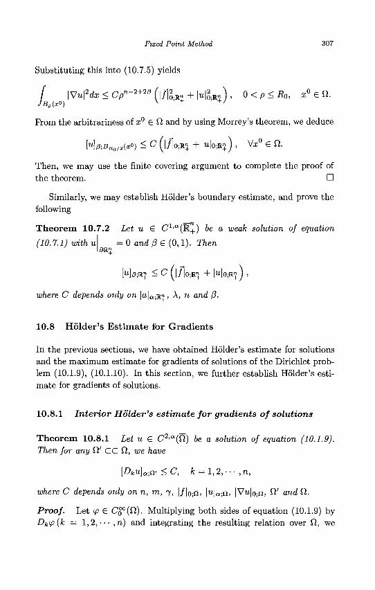
Fixed Point Method 307
/ .
Substituting this into (10.7.5) yields
\Vu\2dx < Cpn-2+2P (1/lg.Rn + |«|g.R») , 0<p<Ro, x ° e O . Bp(x°) \ ' + +/
From the arbitrariness of x° £Q and by using Morrey's theorem, we deduce
M/3;BH0/2(X°) ^ C (l/loiRJ + Mo;R$) , Vx0 € fi.
Then, we may use the finite covering argument to complete the proof of the theorem. •
Similarly, we may establish Holder's boundary estimate, and prove the following
Theorem 10.7.2 Let u G C 1 , a (R + ) be a weak solution of equation
(10.7.1) with u = 0 and/3e (0,1). Then
MfrRJ < C f l/|0jR!f. + MojRIM i
where C depends only on |a|a;Rn, A, n and {3.
10.8 Holder ' s Es t imate for Gradients
In the previous sections, we have obtained Holder's estimate for solutions and the maximum estimate for gradients of solutions of the Dirichlet problem (10.1.9), (10.1.10). In this section, we further establish Holder's estimate for gradients of solutions.
10.8.1 Interior Holder's estimate for gradients of solutions
Theorem 10.8.1 Let u e C 2 ' a (0) be a solution of equation (10.1.9). Then for any il' CCft, we have
[Dku]a.n> < C, fc = l ,2, ••• ,n,
where C depends only on n, m, 7, |/|o ;n, |w|a;n, |Vu|o;n, fi' and Q,.
Proof. Let ip € C£°(ft). Multiplying both sides of equation (10.1.9) by Dk<p{k = 1,2, ••• ,n) and integrating the resulting relation over fi, we
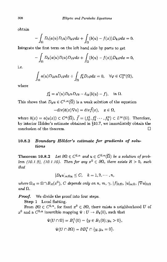
308 Elliptic and Parabolic Equations
obtain
- / Di{a{u)Diu)Dkipdx + / (b(u) - f{x))Dkipdx = 0. Jn Jn
Integrate the first term on the left hand side by parts to get
- / Dk(a(u)Diu)Diipdx+ / (b(u) - f(x))Dktpdx = 0, Jn Jn
i.e.
where
/ a(u)DikuDi<fdx + f fkD^dx = 0, V<p G Cg°(fi), Jn Jn
fk = a'{u)DkuDiU - Sik(b(u) - / ) , in fi.
This shows that Dku G C1,a(fi) is a weak solution of the equation
—div(a(x)Vv) = div/(a;), x G Q,
where a{x) = a(u(x)) G C a(H), / = (/fe\ /fe2 • • • , / £ ) G L°°(fi). Therefore,
by interior Holder's estimate obtained in §10.7, we immediately obtain the conclusion of the theorem. •
10.8.2 Boundary Holder's estimate for gradients of solutions
Theorem 10.8.2 Let dQ, G C2'a and u G C2>a(U) be a solution of problem (10.1.9), (10.1.10). Then for any x° G dQ., there exists R > 0, such that
\Dku\a.QR<C, k = 1,2, ••• ,n,
where CIR = QnBfl(x°), C depends only on n, m, 7, |/|o ;n, |w|Q;n, |Vu|o;n and Q..
Proof. We divide the proof into four steps. Step 1 Local flatting. Prom 9Q G C2'a, for fixed a;0 G dfi, there exists a neighborhood U of
x° and a C 2 , a invertible mapping Vt : U —> Bi(0), such that
9{Unfl) = flftO) = {2/ G Bi(0); j/„ > 0},
y(undn) = dB+n{y;yn = o}.
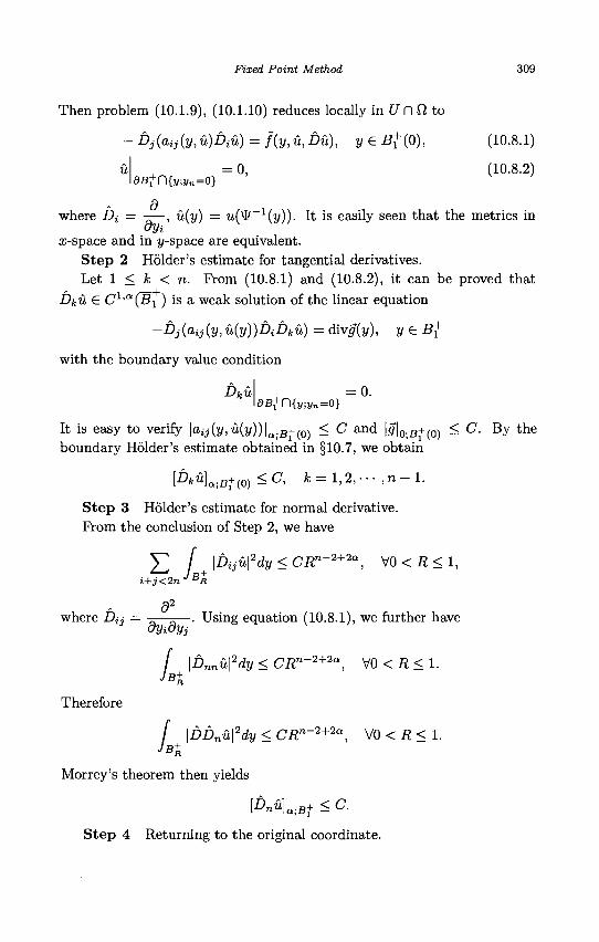
Fixed Point Method 309
Then problem (10.1.9), (10.1.10) reduces locally in U n Q to
-Dj(aij(y,u)Diu) = f(y,u,Du), y € B+(0), (10.8.1)
u = 0 , (10.8.2) dB+r\{y;yn=0}
where Di = -^—, u(y) = u(^/~1(y)). It is easily seen that the metrics in
x-space and in y-space are equivalent. Step 2 Holder's estimate for tangential derivatives. Let 1 < k < n. Prom (10.8.1) and (10.8.2), it can be proved that
is a weak solution of the linear equation
-Dj(aij(y,u(y))DiDku) = divg(y), y € Bf
with the boundary value condition
Dku = 0. dB+n{y;yn=0}
It is easy to verify |a^(y,u(y)) |a ; B+ ( 0 ) < C and |5|0.B+(0) < C. By the boundary Holder's estimate obtained in §10.7, we obtain
[Dku]a.B+{0) < C, fc = l , 2 , - - - , n - l .
Step 3 Holder's estimate for normal derivative. From the conclusion of Step 2, we have
^2 f \Diju\2dy < CRn-2+2a, V0 < R < 1, i+j<2n,'BR
d2
where Da = ——-—. Using equation (10.8.1), we further have dyidyj
L \Dnnu\2dy < CRn~2+2a, V0 < R < 1.
Therefore
/ \DDnu\2dy < CRn-2+2a, V0 < R < 1. JBt
Morrey's theorem then yields
[DnU]a,Bt < C.
Step 4 Returning to the original coordinate.
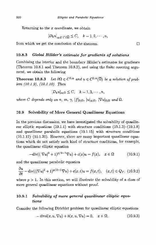
310 Elliptic and Parabolic Equations
Returning to the x coordinate, we obtain
lDku}a]u n n ^ C> k = l,2,---,n,
from which we get the conclusion of the theorem. •
10.8.3 Global Holder's estimate for gradients of solutions
Combining the interior and the boundary Holder's estimates for gradients (Theorem 10.8.1 and Theorem 10.8.2), and using the finite covering argument, we obtain the following
Theorem 10.8.3 Let dfl G C2<a and u G C2'a(Tl) be a solution of problem (10.1.9), (10.1.10). Then
[Dku]a-n <C, k = 1,2, ••• ,n,
where C depends only on n, m, 7, |/|o ;n, |w|a;n, |Vu|o;n and£l.
10.9 Solvability of More General Quasilinear Equations
In the previous discussion, we have investigated the solvability of quasilinear elliptic equations (10.1.1) with structure conditions (10.1.3)-(10.1.8) and quasilinear parabolic equations (10.1.15) with structure conditions (10.1.17)-(10.1.20). However, there are many important quasilinear equations which do not satisfy such kind of structure conditions, for example, the quasilinear elliptic equation
-div(( |Vu|2 + l f / ^ V u ) + c{x)u = f(x), xeQ, (10.9.1)
and the quasilinear parabolic equation
^ - div((|Vu|2 + l ) " / 2 " 1 Vu) + c(x, t)u = f(x, t), (x, t) G QT, (10.9.2)
where p > 1. In this section, we will illustrate the solvability of a class of more general quasilinear equations without proof.
10.9.1 Solvability of more general quasilinear elliptic equations
Consider the following Dirichlet problem for quasilinear elliptic equations
- diva(x,u, Vu) + b{x,u, Vu) = 0, x G Q, (10.9.3)
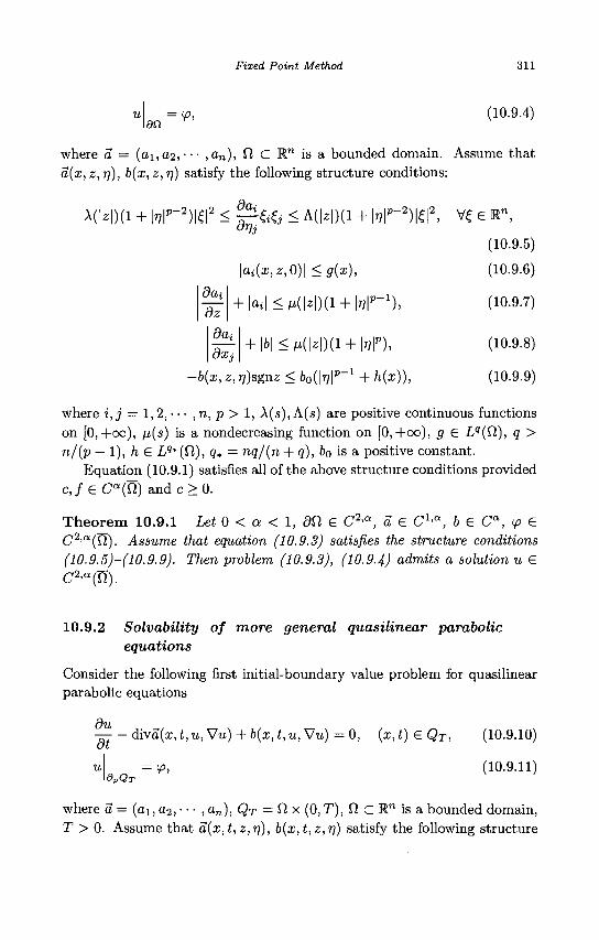
Fixed Point Method 311
an (10.9.4)
where a = (01,02,-•• , a n ) , fl C Rn is a bounded domain. Assume that a(x, z,rf), b(x, Z,TJ) satisfy the following structure conditions:
A(izD(i+\r,r2)\e < f ^ & < A(|Z|)(I+\vr2m2 , ^ e
dai
dz
da dxi
\a,i(x,z,0)\ <g{x),
+ |a i |< /x( |z | ) ( l + | 7 7 r 1 ) ,
+ \b\<VL(\z\){l + \T,n
-b(x, z,r])sgnz < b0(\r)\p 1 + h(x)),
(10.9.5)
(10.9.6)
(10.9.7)
(10.9.8)
(10.9.9)
where i,j = 1,2, • • • ,n, p > 1, A(s), A(s) are positive continuous functions on [0,+00), fi(s) is a nondecreasing function on [0,+00), g G Lq(Q), q > n/(p — 1), h £ Lq* (fi), q* = nq/(n + q), 60 is a positive constant.
Equation (10.9.1) satisfies all of the above structure conditions provided c,f G C a (0 ) a n d c > 0 .
Theorem 10.9.1 Let 0 < a < 1, d£l £ C2'a, a £ C 1 , a , b £ Ca, <p £ C2 'a(fJ). Assume that equation (10.9.3) satisfies the structure conditions (10.9.5)-(10.9.9). Then problem (10.9.3), (10.94) admits a solution u G C2'a(ty.
10.9.2 Solvability of more general quasilinear parabolic equations
Consider the following first initial-boundary value problem for quasilinear parabolic equations
du ~dt
u
- diva(x, i, it, Vzz) + 6(1, £, u, Vu) = 0, (x,t) G QT, (10.9.10)
= ip, (10.9.11) dpQT
where a = (ai, 02, • • • ,a„), QT = O, x (0,T), Q c R" is a bounded domain, T > 0. Assume that a(x,t,z,r]), b(x,t,z,rj) satisfy the following structure
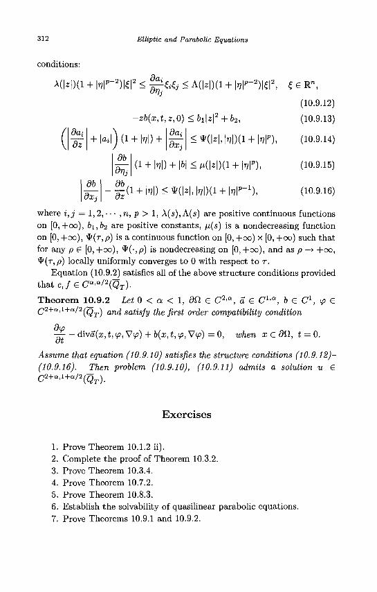
312 Elliptic and Parabolic Equations
conditions:
den \(\z\)(i+\vr
2m2 < ^-tej < A(|ZD(I+\ri\p-2m2, e e Rn,
da<
dz + |Oi|)(l + M) +
96
26(x,i,2,0) <6 i | z | 2 + 62,
dai
dxj <*(W,H)(i + Wp),
96 9x i
dr)j
db
(I + M) + |6 |<M(N)(I + N P ) ,
- ^ ( i + N)<*(N,M)(i + MP+1)
(10.9.12)
(10.9.13)
(10.9.14)
(10.9.15)
(10.9.16)
where i, j = 1,2, • • • , n, p > 1, A(s), A(s) are positive continuous functions on [0,+oo), 61,62 are positive constants, p,(s) is a nondecreasing function on [0, +00), *(r , p) is a continuous function on [0, +00) x [0, +00) such that for any p £ [0, +00), \t(•, p) is nondecreasing on [0, +00), and as p —+ +00, $>(T,P) locally uniformly converges to 0 with respect to r .
Equation (10.9.2) satisfies all of the above structure conditions provided that c,f £Ca'a'2{JQT).
Theorem 10.9.2 Let 0 < a < 1, dfl £ C2>a, a £ C 1 , a , 6 £ C1, <p £ (j2+a,i+a/2^Q^ an^ sansjy foe firsf order compatibility condition
— diva(x, t, <p, V</j) + b(x, t, ip, Vy>) = 0, when x £ 90 , t = 0.
Assume that equation (10.9.10) satisfies the structure conditions (10.9.12)-(10.9.16). Then problem (10.9.10), (10.9.11) admits a solution u £ C 2+a , l+a /2 (Q r )_
Exercises
1. Prove Theorem 10.1.2 ii). 2. Complete the proof of Theorem 10.3.2. 3. Prove Theorem 10.3.4. 4. Prove Theorem 10.7.2. 5. Prove Theorem 10.8.3. 6. Establish the solvability of quasilinear parabolic equations. 7. Prove Theorems 10.9.1 and 10.9.2.
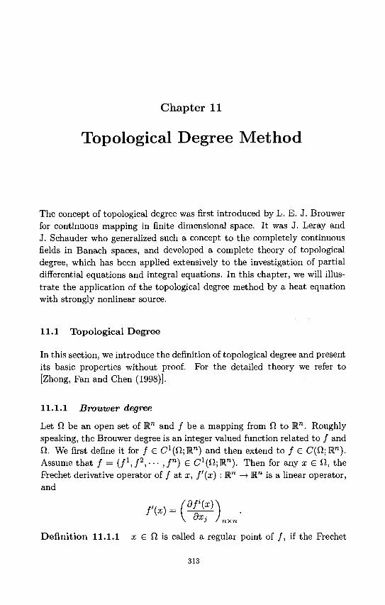
Chapter 11
Topological Degree Method
The concept of topological degree was first introduced by L. E. J. Brouwer for continuous mapping in finite dimensional space. It was J. Leray and J. Schauder who generalized such a concept to the completely continuous fields in Banach spaces, and developed a complete theory of topological degree, which has been applied extensively to the investigation of partial differential equations and integral equations. In this chapter, we will illustrate the application of the topological degree method by a heat equation with strongly nonlinear source.
11.1 Topological Degree
In this section, we introduce the definition of topological degree and present its basic properties without proof. For the detailed theory we refer to [Zhong, Fan and Chen (1998)].
11.1.1 Brouwer degree
Let f2 be an open set of R™ and / be a mapping from fi to Rn . Roughly speaking, the Brouwer degree is an integer valued function related to / and Q.. We first define it for / £ C^fyR") and then extend to / e C(fi;Rn). Assume that / = (Z 1 , / 2 , - - - , / " ) £ C ^ t y R " ) . Then for any x £ ffc, the Frechet derivative operator of / at x, f'(x) : R™ —> R™ is a linear operator, and
\ UXJ / nxn
Definition 11.1.1 x £ 0. is called a regular point of / , if the Frechet
313
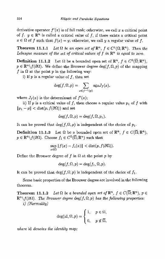
314 Elliptic and Parabolic Equations
derivative operator f'(x) is of full rank; otherwise, we call x a critical point of / . y G R" is called a critical value of / , if there exists a critical point x G Cl of / such that f{x) = y; otherwise, we call y a regular value of / .
Theorem 11.1.1 Let Cl be an open set o/R", f G C^fyR") . Then the Lebesgue measure of the set of critical values of f in R™ is equal to zero.
Definition 11.1.2 Let fibea bounded open set of R", / G C2(fi;R"), p G M.n\f(dCl). We define the Brouwer degree deg(/, Cl,p) of the mapping / in Cl at the point p in the following way:
i) If p is a regular value of / , then set
deg(f,Cl,p) = ] T sgnJ/(x), xef-1(P)
where Jj{x) is the determinant of f'(x); ii) If p is a critical value of / , then choose a regular value p\ of / with
Ibi — p\\ < dist(p, f(dCl)) and set
deg(/,fi,p) = deg(/,fi,pi).
It can be proved that deg(/, Cl,p) is independent of the choice of p\.
Definition 11.1.3 Let Cl be a bounded open set of Rn , / G C(f2;Rn), p G Rn \ / (0I2) . Choose A G C2(fi;R") such that
sup H / f r ) - / i ( aO | |<d i s t (p , / ( 0n ) ) .
Define the Brouwer degree of / in CI at the point p by
deg(/,fi,p) = deg(/i,fi,p).
It can be proved that deg(/, Cl,p) is independent of the choice of f\.
Some basic properties of the Brouwer degree are involved in the following theorem.
Theorem 11.1.2 Let Cl be a bounded open set o/R", / G C(H; R"), p G M.n\f(dCl). The Brouwer degree deg(f,Cl,p) has the following properties:
i) (Normality)
1, pefl,
0, p i fi,
where id denotes the identity map;
deg(id, Cl,p) =
Topological Degree Method 315
ii) (Domain Additivity) Iffli, fi2 o-re two open subsets of tt with Cli D H2 = 0 and p 0 /(H\(Qi U fi2)), then
deg(/,fi,p) = deg(/,fii,p) + deg(/ ,n 2 ,p) ;
raj (Invariance of Homotopy) Let H : fi x [0,1] —> M" 6e a continuous mapping and denote ht(x) = H(x,t). Assume the mapping p : [0,1] —> 1 " is continuous andp(t) £ ht(dfl) for each t 6 [0,1]. Then deg(ht,fl,p(t)) is independent oft.
Based on these basic properties, we may derive a series of important properties of the degree. For example, we have the following theorem.
Theorem 11.1.3 (Kronecker's Existence Theorem) Let Q. be a bounded open set of Rn, f £ C(n;Mn) , p e Rn\/(<9fi). If p £ / (H), then deg(f,Q,p) = 0, and so, if deg(f,Q,p) / 0, then the equation f(x) = p must have at least one solution in Q.
11.1.2 Leray-Schauder degree
Since many problems in analysis are referred to infinite dimensional space, it is natural to extend the Brouwer degree theory to the infinite dimensional case. However, owing to the lack of compactness of the unit ball in the infinite dimensional space, one cannot establish the degree theory for general continuous mappings. It was Leray and Schauder who found an important class of mappings in the investigation of partial differential equations and integral equations, that is the completely continuous perturbations of the identity mappings (also called the compact continuous fields), and applied the method of finite dimensional approximation to establish the degree theory for this class of mappings.
Definition 11.1.4 Let X, Y be two normed linear spaces, D C X, A mapping F : D —> Y is said to be compact, if for any bounded set S C D, F(S) is a compact set in Y. If, in addition, the mapping F is continuous, then we call F a completely continuous mapping or a compact continuous mapping.
Theorem 11.1.4 Let X, Y be two normed linear spaces, M be a bounded closed subset of X. Assume that the mapping F : M —> Y is continuous. If the mapping F is completely continuous, then for any e > 0, there exists a bounded continuous mapping F^ : M —» Yk with finite dimensional range
316 Elliptic and Parabolic Equations
such that
sap \\F(x) - Fk(x)\\ < e,
where Yk CY is a finite dimensional space. Furthermore, if Y is complete, then the above condition is also sufficient.
Definition 11.1.5 Let X be a real normed linear space, D c X. If the mapping F : D —> X is completely continuous, then / = id - F is called a completely continuous field in D, or a compact continuous field in D.
Let X be a real normed linear space, fl be a bounded open set in X, F : tt —> X be a completely continuous mapping, / = id — F be a completely continuous field, p e X\f(dCl). By Theorem 11.1.4, there exist a finite dimensional subspace Xk c X, pk £ Xk and a bounded continuous mapping Fk : Q —» Xk, such that
||p - pfc|| + sup \\F(x) - Fk(x)\\ < dist(p, f(dQ)). x£fl
Denote fife = Xfenft, fk = i d - F k . Then /fc € C(f2fc,Xfe), pk e Xk\fk(dnk), and hence the Brouwer degree deg(/fc,fifc,pfc) is well-defined.
Definition 11.1.6 Define the Leray-Schauder degree of the completely continuous field / in O at the point p by
deg(/,fi,p) =deg(fk,nk,pk).
It can be shown that deg(/, fi, p) is independent of the choice of Xk, pk and Fk.
Since the Leray-Schauder degree is obtained by the approximation of the Brouwer degree, it can be proved that most properties of the Brouwer degree are retained.
Theorem 11.1.5 Let Q be a bounded open subset of X which is a real normed linear space, f = id — F be a completely continuous field on CI, p € X\f(d£l). Then the Leray-Schauder degree deg(/, 0,p) has the following properties:
i) (Normality)
i, pen,
o, P i U-, deg(id,fi,p) =
Topological Degree Method 317
ii) (Domain Additivity) Iftoi, fi2 are two open subsets of to with to\ n 0 2 = 0 andpg /(JT\(fii U to2)), then
deg(/ ,n,p) = deg(/,Qi,p) + deg(/,fl2 ,p);
Hi) (Invariance of Compact Homotopy) Let H : to x [0,1] —» X be a completely continuous mapping and denote ht(x) = x — H(x,t). Assume the mapping p : [0,1] —> X is continuous and p(t) £ ht(dto) for every t G [0,1]. Then deg(ht,to,p(t)) is independent oft.
Theorem 11.1.6 (Kronecker's Existence Theorem) Let X be a real normed linear space, to be a bounded open subset of X, and f = id — F be a completely continuous field defined onto, p £ X\f(dCl). If p $ /(fi) , then deg(/, £l,p) = 0. Thus, i/deg(/,fi,p) =/= 0, then the equation f(x) = p admits at least one solution in fi.
11.2 Existence of a Heat Equation with Strong Nonlinear Source
As an example in applications of the topological degree method, let us consider the heat equation with the strong nonlinear source
^ . - A u = | t i | P , (x,t)£QT (11.2.1)
with the initial-boundary value condition
u(x,t) = >p, {x,t) € dpQT, (11.2.2)
where p > 1, QT = to x (0, T), Q, is a bounded domain in R" with dto G C2'a, a€ (0,1), T > 0 .
If the right hand side of (11.2.1) is a function f(x,t) independent of u, namely, the equation
^ . - A « = / , (x,t)€QT (11-2.3)
is considered, then by the theory of classical solutions for the nonhomo-geneous heat equation, the first initial-boundary value problem (11.2.3), (11.2.2) admits a unique solution u G C2+a'1+a/2(QT) and
\u\2+a,l+a/2;QT ^ C0 (\f\a,a/2;QT + \f\2+a,l+a/2;QT) , (11.2.4)
318 Elliptic and Parabolic Equations
provided / G Ca>a'2{QT), <p G C2+a'1+a/2(QT), where C0 depends only on n, Cl and T. Our aim is to obtain the existence of C2+a'1+a/2(QT) solutions of the first initial-boundary value problem (11.2.1), (11.2.2). To this purpose, we use the topological degree method.
Assume that <p G C2+a<1+a/2(QT). Define a mapping
F : Ca'a'2{QT) x [0,1] ^Ca'a'2(QT),
(/, a) >-m,
where u £ C2+a'1+a^2(QT) is the solution of the problem
UXl
— -Au = crf, (x,t)eQT,
u(x,t)=(p, (x,t)edpQT-
We proceed to show that F is a completely continuous mapping.
Lemma 11.2.1 The mapping F is compact.
Proof. Assume that {fk}f=1 C Ca'a/2(QT), {o-k}f=1 C [0,1] and there exists a constant M > 0, such that
\fk\a,a/2;QT < M, Vfc > 1.
Denote Uk = F(fk,ak), that is uk G C2+a'1+a/2(QT) is the solution of the following problem
—— - Aufc = CTfc/fe, (a;, t) G Qr ,
uk(x,t) = ip, (x,t) £ dpQT-
By virtue of the classical theory, we have
\Uk\2+a,l+a/2;QT ^ ^ 0 (lc rfe/fc|a,a/2;QT + \<P\2+a,l+a/2;QT)
with Co given in (11.2.4), which implies that { u f c } ^ is uniformly bounded in C2+a'1+a/2(QT). Therefore, there exists a convergent subsequence of {uk}k
xL1 in Ca'a/2(QT), this means that the mapping F is compact. •
Lemma 11.2.2 The mapping F is continuous.
Proof._Assume that {fk}?=1 C C a - a / 2 (Q T ) , K } £ ° = 1 C [0,1], / G C a ' " / 2 (Q T ) , a G [0,1], and
Hm |/fc - f\a,a/2;QT = 0, l i m <Jk = a. fc—>oo fc—»oo
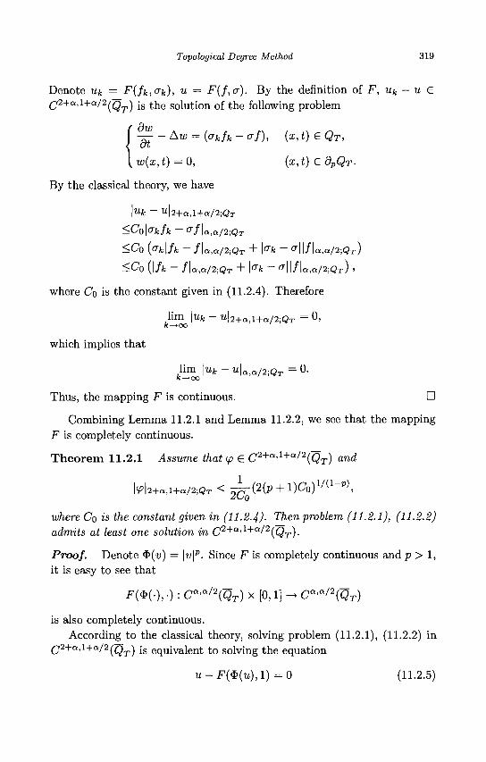
Topological Degree Method 319
Denote uk = F(fk,o-k), u = F(f,a). By the definition of F, uk — u £ (j2+a,i+a/2^Q^ j s fae s o i u t i 0 n of the following problem
— -Aw = (<7fc/fc - af), (x, t) e QT,
w(x,t) = 0, (x,t) e dpQr-
By the classical theory, we have
|Ufc - u\2+a,l+a/2;QT
<CoWkfk - C/U,C*/2;QT
<CQ ((Tfe|/fc - f\aia/2;QT + Wk - 0-||/U,a/2-,QT)
<CQ (|/fc - f\a,a/2;QT + \°~k - ^ | | / | a , a / 2 ; Q T ) ,
where Co is the constant given in (11.2.4). Therefore
which implies that
l im \uk - u\2+a,l + a/2;QT = °> k—>oo
lim \uk - 1iU,a/2;QT = 0. k—»oo
Thus, the mapping F is continuous. •
Combining Lemma 11.2.1 and Lemma 11.2.2, we see that the mapping F is completely continuous.
Theo rem 11.2.1 Assume that (p G C2+a<1+a/2{QT) and
M 2 +a, i+aAQT < ^ ( 2 ( p + l )C 0 ) 1 / ( 1 - p ) ,
where Co is the constant given in (11.2.4). Then problem (11.2.1), (11.2.2) admits at least one solution in C2+a'1+a^2{Q'r).
Proof. Denote $(v) = \v\p. Since F is completely continuous and p > 1, it is easy to see that
F($(- ) ,0 : Ca^2(QT) x [0,1] - Ca^2(QT)
is also completely continuous. According to the classical theory, solving problem (11.2.1), (11.2.2) in
(j2+a,\+a/2(tQ^ j g equivalent to solving the equation
u - F ( $ ( w ) , l ) = 0 (11.2.5)
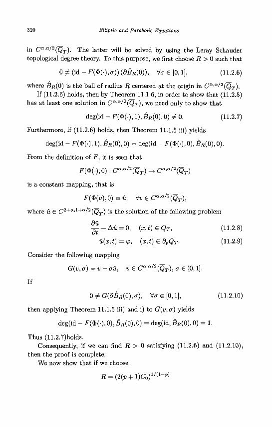
320 Elliptic and Parabolic Equations
in Ca'a/2(QT). The latter will be solved by using the Leray-Schauder topological degree theory. To this purpose, we first choose R > 0 such that
0 ^ ( i d - F ( $ ( - ) , a ) ) ( d B H ( 0 ) ) , V a e [ 0 , l ] , (11.2.6)
where BR(0) is the ball of radius R centered at the origin in Ca>a/2(QT). If (11.2.6) holds, then by Theorem 11.1.6, in order to show that (11.2.5)
has at least one solution in Ca'a^2(QT), we need only to show that
deg(id - F($(-), 1), BR(0), 0) ± 0. (11.2.7)
Furthermore, if (11.2.6) holds, then Theorem 11.1.5 in) yields
deg(id - F($(-), 1), BR(0), 0) = deg(id - F($(•), 0), BR(0), 0).
From the definition of F, it is seen that
F($(-),0) : Ca'a/2(QT) -> Ca>a'2{QT)
is a constant mapping, that is
F{<5>{v),G)=u, Vu e Ca'a/2(QT),
where u € C2+a'l+a^2(QT) is the solution of the following problem
du
— -Au = 0, (x,t)eQT, (11.2.8)
u(x,t) = ip, (x,t) e dpQT. (11.2.9)
Consider the following mapping
G(v,a)=v-au, v£ Ca>a/2(QT), a € [0,1].
If
0^G(dBR(Q),a), VffG[0,l], (11.2.10)
then applying Theorem 11.1.5 iii) and i) to G(v,a) yields
deg(id - F($(-),0),BR(0),0) = deg(id,BR(0),0) = 1.
Thus (11.2.7)holds. Consequently, if we can find R > 0 satisfying (11.2.6) and (11.2.10),
then the proof is complete. We now show that if we choose
R = (2(p + l)C0)1/(1-p)
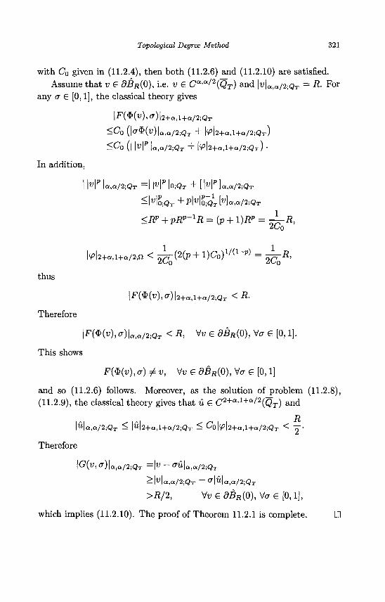
Topological Degree Method 321
with Co given in (11.2.4), then both (11.2.6) and (11.2.10) are satisfied. Assume that v G 8BR{0), i.e. v £ Ca'a^(QT) and
\v\a,a/2;QT = R- F° r
any a S [0,1], the classical theory gives |F($(u),<r) |2 + Q ,1 + a / 2 ; Q T
< C 0 ( k $ ( u ) | Q , a / 2 ; Q T + |y|2+a,l+a/2;QT)
< C 0 (I M P U,a/2;QT + k |2+a, l+a/2;QT ) •
In addition,
I |" |P U,Q/2;QT =1 M" IO;QT + [ MP ]a,a/2;QT
^Mo ;QT + P I W I O ^ 1T H « . « / 2 ; Q T
<flp + p f ip - 1 ^ = (p + i)i?p = - i - f l , zOo
lv |2+a,l+a/2;n < ^ T (2(p + l ) C o ) 1 / ( 1 ~ P ) = ^ R ,
thus
| F ($ (u ) ,CT) | 2 + a , 1 + a / 2 ;Q T < f l .
Therefore
|F($(w),a) | a , a / 2 iQT < fl, Vv e 0B«(O), Vcr e [0,1].
This shows
F($(v) ,a ) ^ w, W e 0B«(O), Vcr € [0,1]
and so (11.2.6) follows. Moreover, as the solution of problem (11.2.8), (11.2.9), the classical theory gives that u S C2+a'1+a/2(QT) and
ma,a/2;QT < \u\2+a,l+a/2;QT ^ Co\<P\2+a,l+a/2;QT < —.
Therefore
\G{v,<?)\a%a/2;QT =\V - Vu\a,a/2;QT
>\v\a,a/2;QT ~ v\u\a,a/2;QT
>R/2, to e 0Bfl(O), Va e [0,1],
which implies (11.2.10). The proof of Theorem 11.2.1 is complete. •
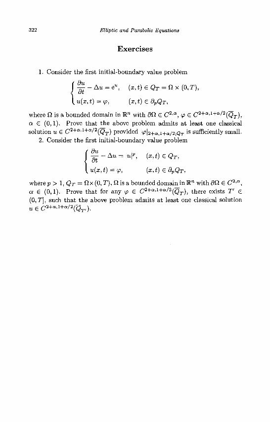
322 Elliptic and Parabolic Equations
Exercises
1. Consider the first initial-boundary value problem
i ^ - A u = eu, (x,t)£QT = Qx(0,T),
[u(x,t) = <p, {x,t)edpQT,
where Q is a bounded domain in Rn with dfi e C2-Q, <p £ C 2 + Q - 1 + a / 2 (Q T ) , a £ (0,1). Prove that the above problem admits at least one classical solution u £ C2+a'1+a/2(QT) provided \<p\2+a,i+a/2;QT
is sufficiently small. 2. Consider the first initial-boundary value problem
f ^ - A u = K> (x,t)£QT,
[u(x,t) = ip, (x,t)£dpQT,
where p > 1, QT = Q x (0, T), fl is a bounded domain in R" with dtt £ C2'a, a £ (0,1). Prove that for any <p £ C2+a'l+a/2(QT), there exists V £ (0,T], such that the above problem admits at least one classical solution u G C 2 + a , l + a / 2 ( Q T , ) .
Chapter 12
Monotone Method
The method of supersolutions and subsolutions is a powerful tool in establishing existence results for differential equations. What is more, this method can also be applied to systems. The basic idea of this method is to use a supersolution or a subsolution as the initial iteration in a suitable iterative process, so that the resulting sequence of iterations is monotone and converges to a solution of the problem. The underlying monotone iterative scheme can also be used for the computation of numerical solutions when these equations are replaced by suitable finite difference equations.
In this chapter, the method of supersolutions and subsolutions and its associated monotone iteration are introduced for a scalar heat equation and a system of coupled heat equations as two typical examples. Similar argument can be applied to the general parabolic equations and systems and also to elliptic equations and systems.
12.1 Monotone Method for Parabolic Problems
We consider the following nonlinear parabolic problem
— - A u = / («) , ( z , t ) e Q r = ftx(0,T), (12.1.1)
u(x,t)=g(x,i), (x,t)edpQT, (12.1.2)
where fl C 1 " is a bounded domain with <9fi G C2<a, f € CQ(R) and g G C2+a'1+c"/2(QT) with some 0 < a < 1. In this chapter, we merely consider classical solutions in C2'1{QT) f~l C(QT).
323
324 Elliptic and Parabolic Equations
12.1.1 Definition of supersolutions and subsolutions
Definition 12.1.1 A function u € C^iQr) n C{QT) is called a super-solution of problem (12.1.1), (12.1.2), if
^-Au>f(u), (x,t)&QT,
u(x, t) > g(x, t), (x, t) e dpQT.
Similarly, a function % £ C2'l{QT) n C(QT) is called a subsolution of problem (12.1.1), (12.1.2) if
du,
-g-Au </(%), (x,t)eQT, &{x, t) < g(x, t), (x, t) S dpQT.
For a supersolution u and a subsolution & of problem (12.1.1), (12.1.2), we say that the pair 'u, % are ordered if
u(x,t) >&(x, t), (x,t) £ QT.
Definition 12.1.2 For any ordered supersolution and subsolution u, &, we define the sector (j/,u) as the functional interval
(%,u) = {u e C(QT);&(x,t) < u(x,t) <u(x,t), (x,t) s QT}.
12.1.2 Iteration and monotone property
It is clear that every solution of problem (12.1.1), (12.1.2) in C2'1(QT) n C{QT) is a supersolution as well as a subsolution. Therefore, supersolutions and subsolutions exist unless the problem has no solution in C2,1(QT) n C(QT). To ensure the existence of a solution it is necessary to impose more condition on the reaction function / . A basic assumption is the following one-sided Lipschitz condition
f(ui) - f(u2) > -c(ui - u2), ^,<u2<ui<u, (12.1.3)
where c is a constant and u, ^ are given ordered supersolution and subsolution. Clearly this condition is satisfied with c = 0 when / is monotone nondecreasing in E. In view of (12.1.3), the function
F(u) = cu + f(u)
is monotone nondecreasing in u for u € (%,ti).
Monotone Method 325
Adding cu on both sides of equation (12.1.1) and choosing a suitable initial iteration u^ £ C2I1(QT)^C(QT), we construct a sequence {u^}'j£=0
successively from the iteration process
duW dt
Au(fc) + cu(fe) = F(u{k~l)), (s, t) £ QT, (12.1.4)
u{k\x,t) =g(x,t), (x,t) £ dpQT. (12.1.5)
Since for each k > 1 the right side of (12.1.4) is known, the 1? theory and the maximum principle guarantee that the sequence {u^}^L0 is well denned. Prom the regularity of solutions of heat equations,
u(l) g Ca,a/2(QT^ u(k) g C2+a,l+a/2(QTj for Jfc = 2 , 3 , • • • .
A natural choice of u^ is u^ = 'u and u^ = Q. Denote the sequences denned by (12.1.4), (12.1.5) with u(°> = u and «(°> = & by {uW}£L0
and {u^}fc^o' an<^ refer to them as the upper sequence and the lower sequence of (12.1.4), (12.1.5), respectively. The following lemma presents the monotone property of these two sequences.
Lemma 12.1.1 Let 'u, & be ordered supersolution and subsolution of problem (12.1.1), (12.1.2) and f satisfy (12.1.3). Then the sequences {u^}£L 0 and {u^}j£Lo Possess the monotone property
u(x, t) = M (0)(x, t) < u(fc)(X) t) < u{k+1)(x, t)
<u{k+1){x,t)<u<-k)(x,t)<rf0){x,t)=u(x,t), {x,t)£~QT (12.1.6)
for every k = 1,2, • • •.
Proof. Let
w(x,t) = u{0){x,t)-u{1)(x,t) =u(x,t)-u(-1)(x,t), (x,t) £~QT.
Then w £ C2,1{QT) H C(QT) is a solution of the problem
^ - A w + cw>F{u)-F(u)=0, (x,t)£QT,
w(x, t) > g(x, t) - g(x, t) = 0, (x, t) £ dvQT-
The maximum principle leads to w > 0 on QT, i.e.
u{1){x,t) < u{0)(x,t) = u(x,t), (x,t) £ QT.
Similarly
i{1)(x,t) >u ( 0 ) (x , t ) =%(x,t), {x,t) £Q T-
326 Elliptic and Parabolic Equations
Let
wil){x,t) = u{1){x,t)-u(-1)(x,t), (x,t) £~QT.
Then w^ e C2'\QT) n C(QT) satisfies
—— _ A ^ 1 ) + gwW = F(u) - F(%) > 0, (x, t) e Q r ,
iu (1)(x,i) = s(z, t) - $ ( s , t ) = 0, (x,t) e 9PQT .
Again, by the maximum principle, u/1) > 0 on QT, i.e.
u ( 1 ) 0M) < u ( 1 )(x,t) , (x,t) e Q r .
Then, we have
u ( 0 ) ( M ) =(%(x,t) <u ( 1 )(a;, i) < u{1)(x,t) < u(x,t) = u^(x,t),
(x,t) e QT.
Suppose
w ( fc_1)(^-0 <U.{k)(x,t) <uw(x,t) < u^k-^(x,t), (x,t) eQT
for some k > 1. Then the function
m ' l » ( i , t ) = i i ' i l ( i , ( ) - 5 ' w l ( i , t ) , ( i , t ) e 5 T
satisfies
5* Aw(fc) + cw(k) = F(rf-k-1)) - F(uk) > 0, (a;, t) € QT,
w<>k) (x, t) = g(x, t) - g{x, t) = 0, (x, t) e dpQT.
The maximum principle implies that w^ > 0 on QT, i.e.
u(k+1){x,t)<u(k)(x,t), (x,t)eQT.
Similar reasoning gives
u{k+1)(x,t)<u{k)(x,t), uik+1)(x,t)<rfk+1)(x,t), (x,t)GQT.
Thus, by induction, the monotone property (12.1.6) follows. •
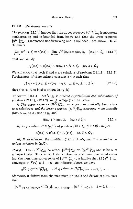
Monotone Method 327
12.1.3 Existence results
The relation (12.1.6) implies that the upper sequence {u^}^=0 is monotone nonincreasing and is bounded from below and that the lower sequence {uSk^}<kLo is monotone nondecreasing and is bounded from above. Hence the limits
lim u(k\x,t) = u(x,t), lim u(k)(x,t) = u(x,t), (x,t) e~QT (12.1.7) k—»oo fc—>oo
exist and satisfy
u(x,t) < u(x,t) < u(x,t) <ti(a;,<), (x, t) G QT.
We will show that both u and u are solutions of problem (12.1.1), (12.1.2). Furthermore, if there exists a constant c< c such that
f(ui) - f{u2) < -c(ui ~u2), &<u2<ui<u, (12.1.8)
then the solution is also unique in (j£,w).
Theorem 12.1.1 Let'u, & be ordered supersolution and subsolution of problem (12.1.1), (12.1.2) and f satisfy (12.1.3). Then
i) The upper sequence {u^}^L0 converges monotonically from above to a solution u and the lower sequence {yLk'}k
xL0 converges monotonically from below to a solution u, and
u(x,t)>u(x,t), {x,t)£QT; (12.1.9)
ii) Any solution u* G (j&,w) of problem (12.1.1), (12.1.2) satisfies
u(x,t) < u*(x,t) <u(x,t), (x,t) G QT;
Hi) If, in addition, the condition (12.1.8) holds, then u = u and is the unique solution in (%,!<)•
Proof. Let {u(fe)}£L0 b e e i t h e r {"(fe)}fcLo o r {u{k))T=o a n d « be u or
u respectively. Since F is Holder continuous and monotone nondecreasing, the monotone convergence of {u^}^L0 to u implies that {F^^^^LQ
converges to F(u) as k —> oo. As indicated above, we have
u ( l ) g Ca,a/2(QT^ „(fc) g C 2 + a , l + a / 2 ( g T ) for fc = 2 , 3 , • • • .
Moreover, it follows from the maximum principle and Schauder's estimate that
|u<*> | 2 + a , l + a / 2 ; Q T < C( | f f l2+a , l+a /2 ;Q T + lU \O-,QT)' fc — 2, 3 , •
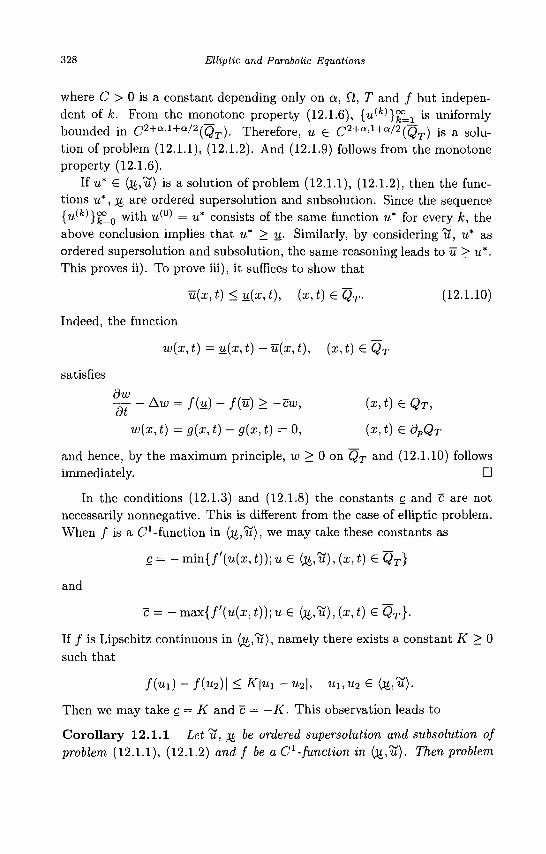
328 Elliptic and Parabolic Equations
where C > 0 is a constant depending only on a, fl, T and / but independent of k. From the monotone property (12.1.6), {u^}'^L1 is uniformly bounded in C2+a<1+a>2{QT). Therefore, u £ C2+a'1+a^2(QT) is a solution of problem (12.1.1), (12.1.2). And (12.1.9) follows from the monotone property (12.1.6).
If u* £ (%,tt) is a solution of problem (12.1.1), (12.1.2), then the functions u*, u are ordered supersolution and subsolution. Since the sequence {^fc)}fclo w ^ t n u ' ° ' = u* c o n s i s t s of the same function u* for every k, the above conclusion implies that u* > u. Similarly, by considering u, u* as ordered supersolution and subsolution, the same reasoning leads to u > u*. This proves ii). To prove hi), it suffices to show that
u(x, t) < u(x, t), (x, t) £ QT. (12.1.10)
Indeed, the function
w(x,t) — u(x, t) - u(x,t), (x,t)eQT
satisfies
—- - Aw = f(u) - f(u) > -cw, (x, t) £ QT,
w(x, t) = g(x, t) - g(x, t) = 0, (x, t) £ dpQT
and hence, by the maximum principle, w > 0 on QT and (12.1.10) follows immediately. •
In the conditions (12.1.3) and (12.1.8) the constants c and c are not necessarily nonnegative. This is different from the case of elliptic problem. When / is a C1-function in (%,'u), we may take these constants as
c = - min{/ ' (u(i , t)); u £ (%, u), (x, t) £ QT]
and
c = -max{/ ' (u (x , t));u£ (%,u), (x,t) 6 QT}.
If / is Lipschitz continuous in (j^t/), namely there exists a constant K > 0 such that
l /("i) - f(u2)\ < K\m -U2\, ui,u2 £ (%,u).
Then we may take c = K and c= —K. This observation leads to
Corollary 12.1.1 Letu, Q be ordered supersolution and subsolution of problem (12.1.1), (12.1.2) and f be a C1 -function in (%,u). Then problem
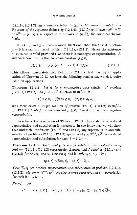
Monotone Method 329
(12.1.1), (12.1.2) has a unique solution in ( J J ,U) . Moreover this solution is the limit of the sequence defined by (12.1.4), (12.1.5) with either u^ = u or u^ = ^ . If f is Lipschitz continuous in (u,ti), the same conclusion holds.
If both / and g are nonnegative functions, then the trivial function Q = 0 is a subsolution of problem (12.1.1), (12.1.2). Hence the existence of solutions is valid provided that there is a nonnegative supersolution. A sufficient condition is that for some constant p > 0,
/ ( p ) < 0 , p>g(x,t), (x,t)£dpQT. (12.1.11)
This follows immediately from Definition 12.1.1 with u = p. By an application of Theorem 12.1.1 we have the following conclusion, which is quite useful in applications.
Theorem 12.1.2 Let H be a nonnegative supersolution of problem (12.1.1), (12.1.2) and f be a C1-function in (0,u). If
/ ( 0 ) > 0 , g(x,t)>0, (x,t)edpQT,
then there exists a unique solution of problem (12.1.1), (12.1.2) in (0,11). If (12.1.11) holds for some constant p > 0, thenH = p is a nonnegative supersolution.
To achieve the conclusion of Theorem 12.1.1, the existence of ordered supersolution and subsolution is necessary. In the following, we will show that under the conditions (12.1.3) and (12.1.8) any supersolution and sub-solution of problem (12.1.1), (12.1.2) are ordered and u^k\ ySk^ are ordered supersolution and subsolution for each k = 1,2, • • •.
Theorem 12.1.3 Let'u and u be a supersolution and a subsolution of problem (12.1.1), (12.1.2) respectively. Assume that f satisfies (12.1.3) and (12.1.8) for any U\ and U2 between)^ andU with u-2 <u\. Then
&(x,t) <'u(x,t), (x,t)eQT.
Thus, 'it, ^ are ordered supersolution and subsolution of problem (12.1.1), (12.1.2). Moreover, vSk\ u^ are also ordered supersolution and subsolution for each k = 1,2, • • •.
Proof. Let
c* = max{|c|, |c|}, w(x,t) ='u(x,t) — $i(x,t), (x,t) £ QT,
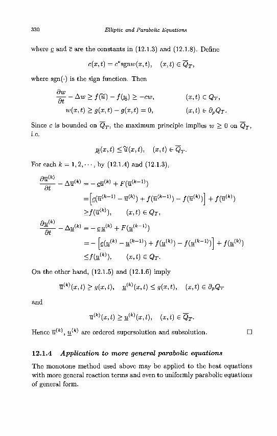
330 Elliptic and Parabolic Equations
where c and c are the constants in (12.1.3) and (12.1.8). Define
c(x, t) = c*sgnw(x,t), (x,t) G QT,
where sgn(-) is the sign function. Then
dw — -Aw> f(u) - /(%) > -cw, (x,t) eQT,
w{x, t) > g(x, t) - g(x, t) = 0, (x, t) G dpQT-
Since c is bounded on QT, the maximum principle implies w > 0 on QT,
i.e.
u(x,t) <u(x,t), (x,t)GQT.
For each k = 1,2, • • •, by (12.1.4) and (12.1.3),
dt
dt
Au<fc> = - c u W + F ( « ( f c - 1 > )
= ~c(u(k~l) - u{k)) + / (n ( f c _ 1 )) - /(u(fc))l + /(u ( fe))
>f(uik)), (x,t)€QT,
Au<fe> cu (fc) F(M(fc_1))
+ /(«' (*h = - c(u(fe) - u^ - 1 ) ) + /(u<fc>) - /(w(fe-1})
</(M(fc)), ( i , t ) € Q r .
On the other hand, (12.1.5) and (12.1.6) imply
u{k)(x,t) > g{x,t), u(k)(x,t) <g(x,t), (x,t) G dpQT
and
u{k){x,t) > u{k)(x,t), (x,t) G QT.
Hence u^k\ u^ are ordered supersolution and subsolution. •
12.1.4 Application to more general parabolic equations
The monotone method used above may be applied to the heat equations with more general reaction terms and even to uniformly parabolic equations of general form.
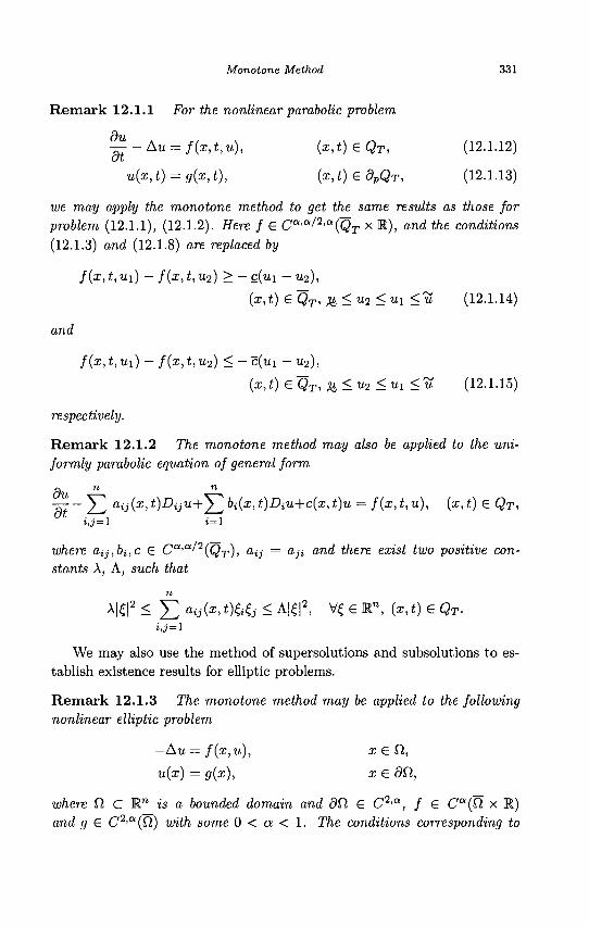
Monotone Method 331
Remark 12.1.1 For the nonlinear parabolic problem
du — -Au = f(x,t,u), (x,t)£QT, (12.1.12)
u(x, t) = g(x, t), (x, t) G dpQT, (12.1.13)
we may apply the monotone method to get the same results as those for problem (12.1.1), (12.1.2). Here f G Ca'a^a(QT x R), and the conditions (12.1.3) and (12.1.8) are replaced by
f(x, t, ui) - f(x, t, u2) > - c(ui - u2),
(x,t) &QT, ^.<u2<u1<u (12.1.14)
and
f(x, t, ui) - f(x, t, u2) < - c(ui - u2), (x,t) £QT, &<u2 < u i < u (12.1.15)
respectively.
Remark 12.1.2 The monotone method may also be applied to the uniformly parabolic equation of general form
p, n n
— - ^2 aij(x,t)Diju+'^2bi(x,t)DiU+c(x,t)u = f(x,t,u), (x,t) G QT, S,J = 1 1 = 1
where aij,bi,c G Ca'a^2(QT), o - = a,ji and there exist two positive constants A, A, such that
n
We may also use the method of supersolutions and subsolutions to establish existence results for elliptic problems.
Remark 12.1.3 The monotone method may be applied to the following nonlinear elliptic problem
—Au = f(x,u), x G f2,
u{x) = g(x), x G dfl,
where Q C Rn is a bounded domain and dfl G C2'a, f G Ca(ft x R) and g G C2'Q(fi) with some 0 < a < 1. The conditions corresponding to
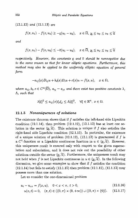
332 Elliptic and Parabolic Equations
(12.1.12) and (12.1.13) are
f(x, Ui ) - f(x, U2) > —c(ui —U2), X € Q, & < U2 < U\ < U
and
f(x,ux) — / (x ,u 2 ) < —c(ui —u2), x € fi, & < u2 < u\ <u
respectively. However, the constants c and c should be nonnegative due to the same reason as that for linear elliptic equations. Furthermore, this method may also be applied to the uniformly elliptic equation of general form
-aij(x)DijU + bi(x)DiU + c(x)u = f(x,u), x € f2,
where aij,bi,c € Ca(Cl), aij = ajj and there exist two positive constants X, A, such that
A|£|2 < OijWZitj < A|£|2, V£ e l " , i e Q.
12.1.5 Nonuniqueness of solutions
The existence theorem shows that if / satisfies the left-hand side Lipschitz condition (12.1.14), then problem (12.1.12), (12.1.13) has at least one solution in the sector (%,'u}. This solution is unique if / also satisfies the right-hand side Lipschitz condition (12.1.15). In particular, the existence of a unique solution of problem (12.1.12), (12.1.13) is guaranteed if / is a C1-function or a Lipschitz continuous function in u S (%,t/). However, this uniqueness result is ensured only with respect to the given superso-lution and subsolution, and it does not rule out the possibility of other solutions outside the sector (%,tt). Furthermore, the uniqueness result may not hold when / is not Lipschitz continuous in u £ (u,u). In the following discussion, we give some examples to show that if / satisfies the condition (12.1.14) but fails to satisfy (12.1.15) then problem (12.1.12), (12.1.13) may possess more than one solution.
Let us consider the one-dimensional problem
Ut ^xx = f(x, u), 0 < x < 7r, t > 0, (12.1.16)
u(x,t) = 0, (x,t)£ ({0,TT}X (0,+oo))U((0,7r)x {O}). (12.1.17)
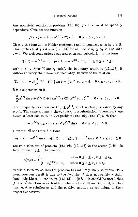
Monotone Method 333
Any nontrivial solution of problem (12.1.16), (12.1.17) must be spatially dependent. Consider the function
f(x,u) = u + 3sin2 / 3(x/2)u1 / 3 , 0 < x < n, u £ R.
Clearly this function is Holder continuous and is nondecreasing in u £ R. This implies that / satisfies (12.1.14) for all - c o < u-i < u\ < +oo with c = 0. We seek some ordered supersolution and subsolution of the form
u{x, t) = pt3/2 sinx, %(x, t) = -pt3/2 sinx, 0 < x < ir, t > 0
with p > 1. Since H and Q satisfy the boundary condition (12.1.17), it suffices to verify the differential inequality. In view of the relation
t£t -ruxx = P ( T ^ 1 / 2 + t3/2j sin a; = -pt1/2 sinx+ u, 0 < x < IT, t > 0,
'u is a supersolution if
-ptl/2smx + u > u + 3sin 2 / 3(x/2)(^ 3 / 2sina;) 1 / 3 , 0 < x < ir, t > 0.
This inequality is equivalent to p > p1^3, which is clearly satisfied by any p > 1. The same argument shows that ^ is a subsolution. Therefore, there exists at least one solution u of problem (12.1.16), (12.1.17) such that
-pt3/2 sin x<u(x,t) < pt3/2 sin x, 0 < x < n, t > 0.
However, all the three functions
ui(x,t) = — t3 / /2sinx, u2(x,t) = 0, u3(x,t) = £3/2sinx, 0 < x < 7 r , t > 0
are true solutions of problem (12.1.16), (12.1.17) in the sector (0,u). In fact, for each to > 0 the function
( 0, when 0 < x < n, 0<t<to, u(x,t) = <
{ (t — to) ' sinx, when 0 < x < n, t > to
is also a solution, so that the problem has infinitely many solutions. This nonuniqueness result is due to the fact that / does not satisfy a right-hand side Lipschitz condition (12.1.15) in (0,u). It should be noted that / is a C1-function in each of the intervals (—co,0) and (0,+co), so that the negative solution u\ and the positive solution u$ are unique in their respective sectors.
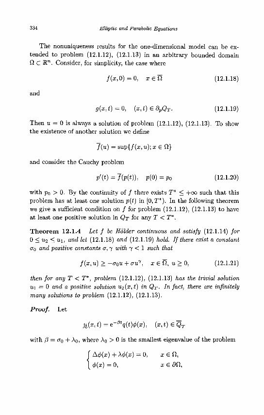
334 Elliptic and Parabolic Equations
The nonuniqueness results for the one-dimensional model can be extended to problem (12.1.12), (12.1.13) in an arbitrary bounded domain f l c l " . Consider, for simplicity, the case where
/ (x ,0) = 0, x e O (12.1.18)
and
g(x, t) = 0, (x, t) £ dpQT. (12.1.19)
Then u = 0 is always a solution of problem (12.1.12), (12.1.13). To show the existence of another solution we define
f{u) = sup{/(z, u)\ x € Q}
and consider the Cauchy problem
p'(t)=J(p(t)), P(0)=Po (12.1.20)
with po > 0. By the continuity of / there exists T* < +oo such that this problem has at least one solution p(t) in [0, T*). In the following theorem we give a sufficient condition on / for problem (12.1.12), (12.1.13) to have at least one positive solution in QT for any T < T*.
Theorem 12.1.4 Let f be Holder continuous and satisfy (12.1.14) for 0 < «2 < u\, and let (12.1.18) and (12.1.19) hold. If there exist a constant (To and positive constants a, 7 with 7 < 1 such that
f(x,u)>-o-0u + aur, xeQ,u>0, (12.1.21)
then for any T < T*, problem (12.1.12), (12.1.13) has the trivial solution u\ = 0 and a positive solution U2{x,t) in QT- In fact, there are infinitely many solutions to problem (12.1.12), (12.1.13).
Proof. Let
)i(x,t) = e-fitq(t)<f>(x), (x,t)GQT
with /3 = (T0 + Ao, where Ao > 0 is the smallest eigenvalue of the problem
Acf)(x) + \<f>(x) = 0, x e d ,
<j>(x) = 0 , x£ dfl,
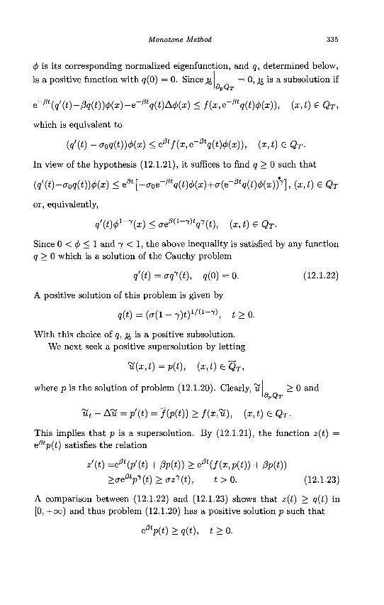
Monotone Method 335
(p is its corresponding normalized eigenfunction, and q, determined below,
is a positive function with q(0) = 0. Since ^ = 0, ^ is a subsolution if 9VQT
e^t(q'(t)-pq(t))(p(x)-e->3tq(t)Act>(x) < / ( i . e ^ ^ t ) ^ ) ) , (x,t) € QT,
which is equivalent to
(q'(t) - aQq{t))4>{x) < ePffae-VqltMx)), (x,t) e QT-
In view of the hypothesis (12.1.21), it suffices to find q > 0 such that
(q'(t)-a0q(t))4>(x) < ^t[-aoe-0tq{t)cj>{x)+a{^tq{t)4>{x)fl (x,t) € QT
or, equivalently,
q'iW'-^x) < ae^-^q^t), (x, t) e QT-
Since 0 < (j) < 1 and 7 < 1, the above inequality is satisfied by any function q > 0 which is a solution of the Cauchy problem
q'(t)=aq-i(t), q(0) = 0.
A positive solution of this problem is given by
?(i) = (<r ( l - 7 )*) 1 / ( 1 ~ 7 ) , * > 0 .
With this choice of q, ^ is a positive subsolution. We next seek a positive supersolution by letting
u(x,t)=p(t), {x,t)GQT,
where p is the solution of problem (12.1.20). Clearly, ti
(12.1.22)
dpQr > 0 and
ut - AH = p'(t) = f(p(t)) > fix,*), (x, t) G QT.
This implies that p is a supersolution. By (12.1.21), the function z(t) = e0tp{t) satisfies the relation
*'(*) =e<}t(p'(t) + 0p(t)) > e^(f(x,p(t)) + (3p(t))
^o-e^V^) > vz^it), t > 0. (12.1.23)
A comparison between (12.1.22) and (12.1.23) shows that z(t) > q(t) in [0, +00) and thus problem (12.1.20) has a positive solution p such that
eptp(t) > q(t), t > 0.
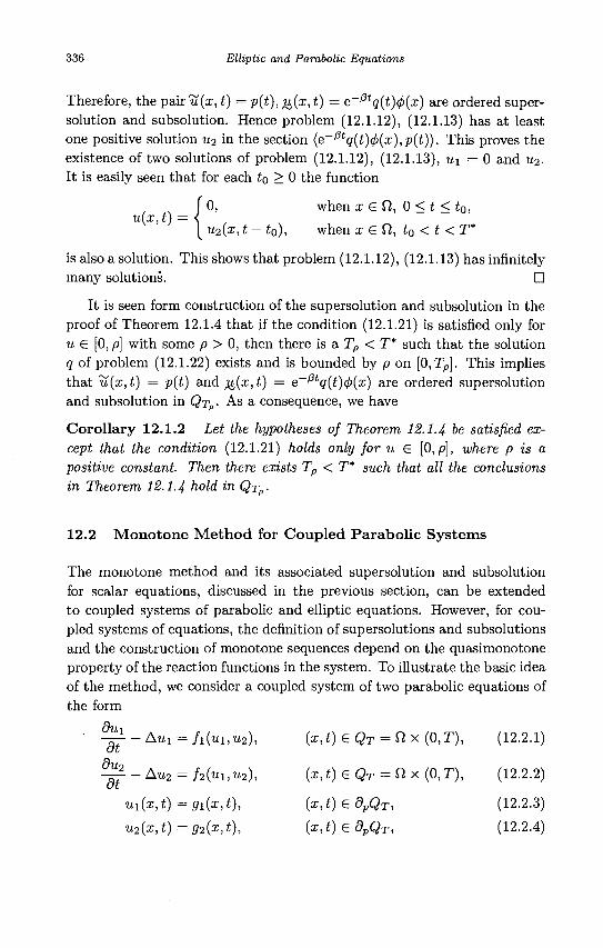
336 Elliptic and Parabolic Equations
Therefore, the pair it (a;, t) = p(t), u(x, t) = e~/3tq(t)4>(x) are ordered super-solution and subsolution. Hence problem (12.1.12), (12.1.13) has at least one positive solution u2 in the section (e~,3tq(t)(j)(x),p(t)). This proves the existence of two solutions of problem (12.1.12), (12.1.13), u\ = 0 and u2. It is easily seen that for each to > 0 the function
/ f 0, when x G ft, 0 < t < t0, u(x,t) = <
[ u2(x, t-t0), when x e ft, t0 < t < T*
is also a solution. This shows that problem (12.1.12), (12.1.13) has infinitely many solutions. •
It is seen form construction of the supersolution and subsolution in the proof of Theorem 12.1.4 that if the condition (12.1.21) is satisfied only for u £ [0, p] with some p > 0, then there is a Tp < T* such that the solution q of problem (12.1.22) exists and is bounded by p on [0,TP], This implies that 'u(x,t) = p(t) and ,%(£,£) = e~^tq(t)(j)(x) are ordered supersolution and subsolution in QTP • As a consequence, we have
Corollary 12.1.2 Let the hypotheses of Theorem 12.1.4 be satisfied except that the condition (12.1.21) holds only for u € [0, p], where p is a positive constant. Then there exists Tp < T* such that all the conclusions in Theorem 12.1.4 hold in QT„-
12.2 Monotone Method for Coupled Parabolic Systems
The monotone method and its associated supersolution and subsolution for scalar equations, discussed in the previous section, can be extended to coupled systems of parabolic and elliptic equations. However, for coupled systems of equations, the definition of supersolutions and subsolutions and the construction of monotone sequences depend on the quasimonotone property of the reaction functions in the system. To illustrate the basic idea of the method, we consider a coupled system of two parabolic equations of the form
/ i(«i ,«2), ( x , i ) e Q T = ftx(0,T), (12.2.1)
/2(ui ,u2) , ( z , t ) e Q T = ftx(0,T), (12.2.2)
gi(x,t), (x,t)edpQT, (12.2.3)
g2(x,t), {x,t)£dpQT, (12.2.4)
dui
du2
~dt Au2 =
ux{x,t) =
u2(x,t) =
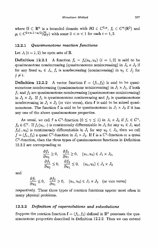
Monotone Method 337
where 0 C R" is a bounded domain with dil G C2>a, fi G CQ(R2) and gi 6 C2+a'1+c,/2{QT) with some 0 < a < 1 for each i = 1,2.
12.2.1 Quasimonotone reaction functions
Let Jj (i = 1,2) be open sets of R.
Definition 12.2.1 A function fi = / i (u i ,u 2 ) (i = 1,2) is said to be quasimonotone nondecreasing (quasimonotone nonincreasing) in J\ x Ji if for any fixed ut £ J,, /» is nondecreasing (nonincreasing) in Uj G Jj for
Definition 12.2.2 A vector function f = ( / i , / 2 ) is said to be quasimonotone nondecreasing (quasimonotone nonincreasing) in J\ x J2, if both f\ and fi are quasimonotone nondecreasing (quasimonotone nonincreasing) in J\X Ji. If / i is quasimonotone nonincreasing and / 2 is quasimonotone nondecreasing in J\ x Ji (or vice versa), then f is said to be mixed quasimonotone. The function f is said to be quasimonotone in J\ x Ji if it has any one of the above quasimonotone properties.
As usual, we call f a C7-function (0 < 7 < 1) in J\ x Ji if /1 G C, fi G C 7 . If fi(u\, •) is continuously differentiable in J2 for any u\ G J\ and /2(-,u2) is continuously differentiable in J\ for any u2 G J2, then we call / = (/i) fi) a quasi C1-function in J\ x J2 . If f is a C1-function or a quasi C1-function, then the three types of quasimonotone functions in Definition 12.2.2 are corresponding to
| ^ - > 0 , | ^ > 0 , (ui.ua) G J i x J2,
| ^ < 0 , | ^ < 0 , (ui.ua) € J i x J2 oui oui
and
-— < 0, —— > 0, (ui,u2) G J\ x Ji (or vice versa) ou2 au\
respectively. These three types of reaction functions appear most often in many physical problems.
12.2.2 Definition of supersolutions and subsolutions
Suppose the reaction function f = ( / i , / 2 ) defined in K2 possesses the quasimonotone properties described in Definition 12.2.2. Then we can extend
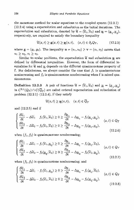
338 Elliptic and Parabolic Equations
the monotone method for scalar equations to the coupled system (12.2.1)-(12.2.4) using a supersolution and subsolution as the initial iterations. The supersolution and subsolution, denoted by u = (Si,ti2) and ji = (ji,,^0), respectively, are required to satisfy the boundary inequality
u(x,t)>g{x,t)>)i(x,t), (x,t)edpQT, (12.2.5)
where g = (31,32)- The inequality u = (u\,u2) > v = (vi,v2) means that Wl > U2, Vi > V2.
Similar to scalar problems, the supersolution u and subsolution yi are defined by differential inequalities. However, the form of differential inequalities for u and u depends on the different quasimonotone property of f. For definiteness, we always consider the case that /1 is quasimonotone nonincreasing and f2 is quasimonotone nondecreasing when f is mixed quasimonotone.
Definition 12.2.3 A pair of functions u = (ui, W2) and JJ = (%,,,%2) in C2,1(QT) n C(QT) are called ordered supersolution and subsolution of problem (12.2.1)-(12.2.4), if they satisfy
u(x,t) >)i(x,t), (x,t) eQT
and (12.2.5) and if
' Bui du — - Aui - / I ( U I , B J ) > 0 > -Q± - A ^ - fi(%vu2),
^ - Au2 - f2{uuu2) > 0 > ^ - A^ 2 - f2(Mv&2),
when {fi,f2) is quasimonotone nondecreasing;
( ^ - Aui - /i(Si,Ai2) > 0 > ^ - A t t l - h{jivu2),
^ - Au2 - f2(%vu2) > 0 > ^ - A ^ - f2(uu^),
when (fi,f2) is quasimonotone nonincreasing; and
^ - A«i - / i («i ,& 2) > 0 > % - - A ^ - h(&vu2\
^ - A« 2 - / 2 (u i , « 2 ) > 0 > ^ - A^ 2 - j ^ , ^ ) ,
(x,t) e Q r
(12.2.6)
(a:,*) € Q T
(12.2.7)
(a:,*) £ < 5 T
(12.2.8)
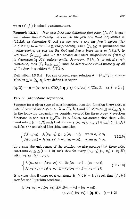
Monotone Method 339
when (/ i , /2) is mixed quasimonotone.
Remark 12.2.1 It is seen from this definition that when ( / i , /2) is quasimonotone nondecreasing, we can use the first and third inequalities in (12.2.6) to determine u and use the second and the fourth inequalities in (12.2.6) to determine ji independently; when ( / i , /2) is quasimonotone nonincreasing, we can use the first and fourth inequalities in (12.2.7) to determine (ui,^ ) and use the second and third inequalities in (12.2.7) to determine (^,,^2) independently. Moreover, if{f\,f2) is mixed quasimonotone, then (u 1,'it2,&,,&?) must be determined simultaneously by all of the four inequalities in (12.2.8).
Definition 12.2.4 For any ordered supersolution u = (wi,W2) and sub-solution JJ = (j&1,2i2), we define the sector
(JJ,U) = {u = (ui,u2) € C{QT);)i(x,t) <u(x,t) <u(x,t), (x,t) e QT).
12.2.3 Monotone sequences
Suppose for a given type of quasimonotone reaction function there exist a pair of ordered supersolution u = (ui,H2) and subsolution JJ, = (J41,^i2). In the following discussion we consider each of the three types of reaction functions in the sector ( J J , U ) . In addition, we assume that there exist constants c, (i = 1,2) such that for every (ui,u2), (vi,v2) G (jj ,u), (fi,f2) satisfies the one-sided Lipschitz condition
j fi(u1,u2)-fi(vi,u2)>-c1(u1-v1), w h e n u i > u i , ( 1 2 2 q \
\ /2(ui ,U2) - h(ui,v2) > -c2(u2 -v2), whenu2 >v2.
To ensure the uniqueness of the solution we also assume that there exist constants ct < ci (i = 1,2) such that for every (u\, u2), {v\,v2) G (u ,u) with (ui,u2) > (vx,v2),
f h(ui,u2) - fi(v1,v2) < - c i ( ( u i -vi) + {u2-v2)),
\f2{ui,U2) - f2(vi,V2) < - C 2 ( ( w i -V1) + (u2 -V2)).
It is clear that if there exist constants Ki > 0(i = 1,2) such that (fi,f2) satisfies the Lipschitz condition
\fi{ui,u2) - fi(vi,v2)\ <Ki(\ui -vi\ + \u2 -v2\),
(ui,u2),(vi,v2)G{fi,u), (i = l,2)
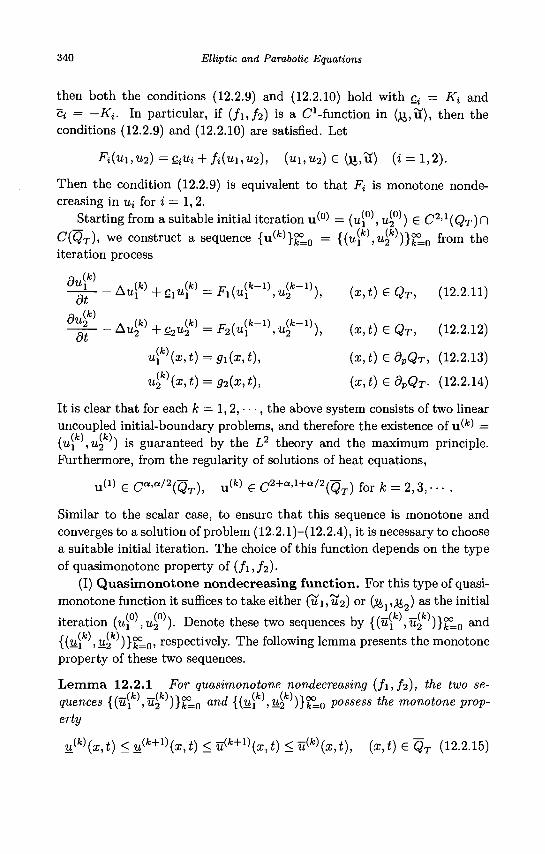
340 Elliptic and Parabolic Equations
then both the conditions (12.2.9) and (12.2.10) hold with c4 = Kt and Ci •= -Ki. In particular, if (fi,f2) is a C^-function in ( J J , U ) , then the conditions (12.2.9) and (12.2.10) are satisfied. Let
Fi(ui,u2) = ciui +fi(ui,u2), (ui,u2) G (JJ,U) (i = 1,2).
Then the condition (12.2.9) is equivalent to that Fi is monotone nonde-creasing in Uj for i = 1,2.
Starting from a suitable initial iteration u'°) = ( 4 , 4 ) G C2,1(QT) fl C(QT), we construct a sequence {uW}£L0 = {(u[k) ,u2
k))}%L0 from the iteration process
^ - A^ f c ) +cAk) = Fi(«i*-1 ) , i4*~1 )), («,*) € Or , (12-2.11)
^ - - A4 f c ) + c24 fc ) = F 2 (4 f c - 1 ) , 4 f c - 1 ) ) , (*,*) G QT, (12.2.12)
u[ f c )(a: ) t)=51(x,t) , (x,t) G dpQT, (12.2.13)
4 * W ) = <72(x,0, ( s , t ) G d p Q r . (12.2.14)
It is clear that for each k = 1,2, • • •, the above system consists of two linear uncoupled initial-boundary problems, and therefore the existence of u(fe) = ( 4 , 4 ) is guaranteed by the L2 theory and the maximum principle. Furthermore, from the regularity of solutions of heat equations,
u ( l ) £ Ca,a/2(QT^ u(fc) g C 2 + a , l + a / 2 ( g r ) for jfc = 2, 3 , • • • .
Similar to the scalar case, to ensure that this sequence is monotone and converges to a solution of problem (12.2.1)-(12.2.4), it is necessary to choose a suitable initial iteration. The choice of this function depends on the type of quasimonotone property of (fi,f2).
(I) Quasimonotone nondecreasing function. For this type of quasi-monotone function it suffices to take either (^1,^2) or (%1,^2) as the initial
iteration (u[ ,u2 ). Denote these two sequences by {(u[ ,u2 )}fc^0 anc^
{ ( 4 , 4 )}S£o' respectively. The following lemma presents the monotone property of these two sequences.
Lemma 12.2.1 For quasimonotone nondecreasing {fi,f2), the two sequences {(u\ ,u2 )}fcL0
and { ( 4 ' 4 )}A^=O possess the monotone property
u{k){x,t) <u{k+1){x,t) < rfk+1\x,t) <rfk\x,t), {x,t)eQT (12.2.15)
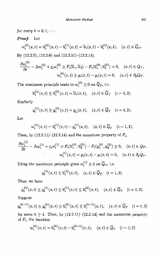
Monotone Method 341
for every k = 0,1,- • •.
Proof. Let
wf (x,t) = ^ 0 ) ( x , i ) - u ^ f o t ) = u i(x, t) - u f ^ x , * ) , ( a ; , t ) 6 Q r .
By (12.2.5), (12.2.6) and (12.2.11)-(12.2.14),
a (0)
2 g - - A w f + Qiwl0) > Fifafa) - F i O E ^ . u f ) = 0, (x, t) e Q r ,
^ i 0 )(x, i ) > 9i(x,t) - gi{x,t) =0, (x,t) £ dpQT-
The maximum principle leads to w\' > 0 on Q r , i.e.
^ 1 ) ( x , t ) < t l f ) ( x , t ) = u i ( x , 0 , ( i , t ) 6 Q r (» = 1,2).
Similarly
l i i 1 ) ( s , t ) > « i 0 ) ( a : , t ) = ^ > t ) , ( x , i ) e Q T (i = 1,2).
Let
^ ( i , t ) = ^ 1 ) ( x , t ) - J i | 1 ) (*.*). 0 M ) e Q r (i = l ,2).
Then, by (12.2.11)-(12.2.14) and the monotone property of Fu
a (i)
*%- - Aw'* + * « , « = Fi(uf\u^) - f i f c i 0 ^ ) > 0, (x,t) e QT,
w(f)(x,t)=gi{x,t)-gi(x,t)=Q, (x,t) € dpQT-
Using the maximum principle gives w\ ' > 0 on QT, i.e.
v^\x,t) < u f } ( x , i ) , ( x , t ) e Q T (i = 1,2).
Thus, we have
u{°)(x,t)<y^1)(x,t)<u\1){x,t)<u{°){x,t), (x,t)£QT (i = 1,2).
Suppose
v^h~1)(x,t)<^k\x,t)<u\k\x,t)<u\k-1)(x,t), {x,t)eQT (i = 1,2)
for some k > 1. Then, by (12.2.11)-(12.2.14) and the monotone property of Fi, the function
wf\x,t)=u{k\x,t)-uf+l\x,t), (x,t)eQT (t = l ,2)
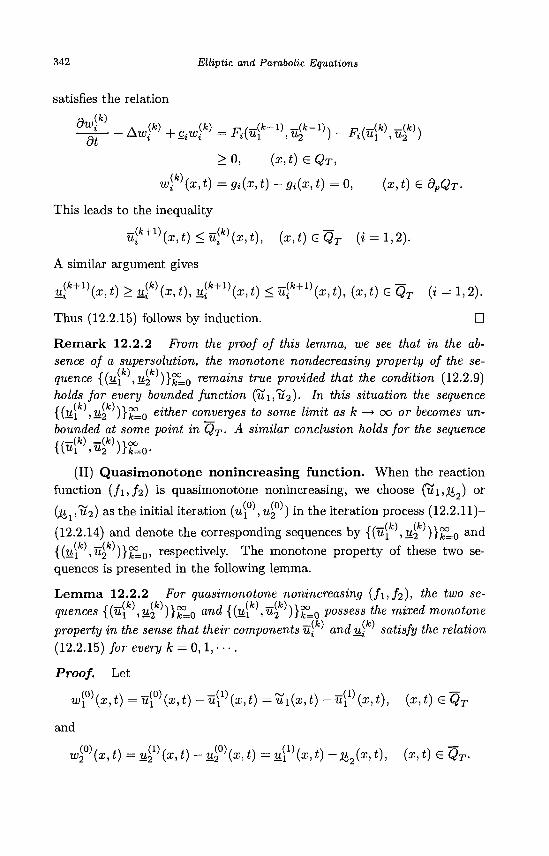
342 Elliptic and Parabolic Equations
satisfies the relation
dt — Awl + £iw
wl (x
,(*) *
,*)
= Fi(v
>o, = 9i(x
(fe-i)
(x,
, * ) -
_ ( f c -, " 2
, * ) 6
St fa,
"V <3T,
.*) = 0
)-Fi(u[k\4k))
(x,t) G 9p<5r-
This leads to the inequality
w f + 1 ) f a , i ) < u f W ) , (x,t)GQT (i = 1,2).
A similar argument gives
«f+1)(M) > « f W ) , «ife+1)(M) <sf+1)fa.*)> fa.*) e QT (* = i>2).
Thus (12.2.15) follows by induction. D
Remark 12.2.2 From the proof of this lemma, we see that in the absence of a supersolution, the monotone nondecreasing property of the sequence {(u[ ,u2 )}fcLo remains true provided that the condition (12.2.9) holds for every bounded function (u1,U2)- In this situation the sequence {bA >I*2 )}fc =o either converges to some limit as k —> 00 or becomes unbounded at some point in QT. A similar conclusion holds for the sequence
{(u[k)M2k))}?=o-
(II) Quasimonotone nonincreasing function. When the reaction
function ( / i , /2) is quasimonotone nonincreasing, we choose (ui,%) or
(ju ,^2) as the initial iteration (u[ ,u2 ) in the iteration process (12.2.11)—
(12.2.14) and denote the corresponding sequences by {(u\ ',u2 )}j^L0 and {(^1 >*4 )}/K=o> respectively. The monotone property of these two sequences is presented in the following lemma.
Lemma 12.2.2 For quasimonotone nonincreasing ( / i , /2) , the two sequences {(u\ ,u2 )}feLo and {(wj ,u 2 ) } ^ o Possess the mixed monotone property in the sense that their components u\ ' and u- satisfy the relation (12.2.15) for every k = 0, ! , - •• .
{°\x,t) =u(i\x,t) - u?\x,t) = u1(x,t)-u{1\x,t), (x,t) G QT
Proof. Let
w
and
w^\x,t)=u2l,(x,t)-u2
u>(x,t)=u\1,(x,t) -%Jx,t), (x,t) G QT.
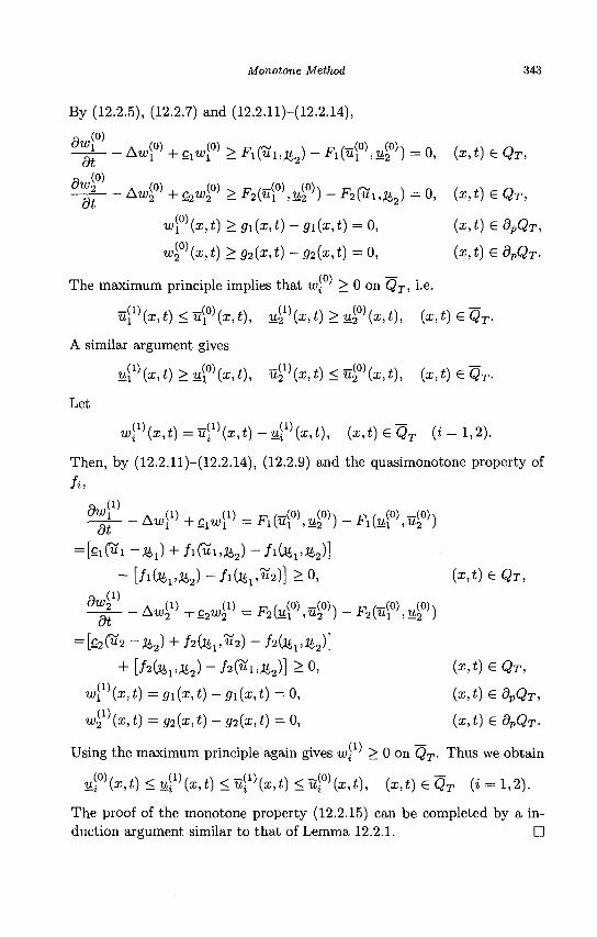
Monotone Method 343
By (12.2.5), (12.2.7) and (12.2.11)-(12.2.14),
^ i - - Aii;<0) + S l < } > F ^ u J - Fi( izi0 ) ,^0 )) = 0, (x,t) e QT,
a (0)
^ g - - A w f + c 2 ^ 0 ) > F2(uf\u20)) - F 2 (» i , % 2 ) = 0, (*, t) e Q r >
wf\x,t) > gi(x,t) - gi{x,t) = 0, (z,£) edpQT,
w20)(x,t) >g2(x,t) -g2(x,t) = 0, (z,t) e dpQT-
The maximum principle implies that u; > 0 on QT, i.e.
i Z ^ f o t J ^ u ^ a : , * ) , r^X) (ar, t) > u^0) (ar, t), (x,t) €QT.
A similar argument gives
u<i\x,t)>uf\x,t), u{2\x,t) <u2
0)(x,t), (x,t) &QT.
Let
w\1\x,t) = uli1)(x,t)-y^1\x,t), {x,t)eQT (i = 1,2).
Then, by (12.2.11)-(12.2.14), (12.2.9) and the quasimonotone property of
Jii
3Wl A (1) , (1) n / - (0) (0)\ ^ / (0) - ( 0 ) \ —^ AwJ ; + c l W i ; = Fi(u\ ',u2 ') - F i ( u i ' , ^ ' )
= [ei(wi-Ai1) + / i ( w i , A i 2 ) - / i f e 1 ^ 2 ) ]
+ [ / iC^i^a) - / I ^ , « 2 ) ] > 0, ( i , t ) e Q r ,
- A«,<» + e r f = FM0)A0)) - ^(Bi0).s40)) rf}
at = [C2(W2 ~ ^ 2 ) + J ^ , ^ ) - f2(UvJh2)]
+ [f2&vJl2) - f2<Vi,H2)] > 0, (x,t) G Q r ,
t o ^ (a;, i) =gi(a;,t) -5i(o; , t ) = 0 , (z,£) € dpQr,
w2 (a;,*) = 02OM) -g2{x,t) = 0, (x,i) e 9PQT .
Using the maximum principle again gives wj ' > 0 on QT. Thus we obtain
«J0)(a;,t) < tij^(a;,t) < tZ^1'(a:,t) < u^0)(x,t), (x,t) &QT (t = l ,2) .
The proof of the monotone property (12.2.15) can be completed by a induction argument similar to that of Lemma 12.2.1. •
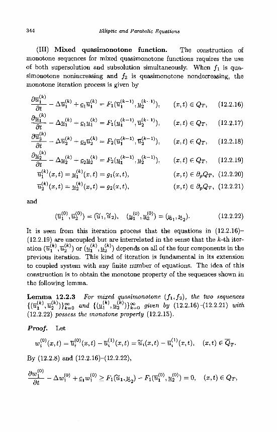
344 Elliptic and Parabolic Equations
(III) Mixed quasimonotone function. The construction of monotone sequences for mixed quasimonotone functions requires the use of both supersolution and subsolution simultaneously. When / i is quasimonotone nonincreasing and f2 is quasimonotone nondecreasing, the monotone iteration process is given by
T ( * ) ^-^+c1ur=Fl{uri)Jti\ ,(k)
dU\ A (k) , (k) „ , (fc-1) _(fc-l)\
a* du\ (k)
dt Au(k) + c2u
{2k) F2{urL\uri>),
-^+c24k)=F2(ut1\ut\
dt
u[k'(x,t) = Ui(x,t) = gi(x,t),
7(fc)/ (x,t) = u2k)(x,t) =g2(x,t),
x,t) € QT,
x,t) e Q T ,
a:,*) e Q T ,
(12.2.16)
(12.2.17)
(12.2.18)
x,t)GQT, (12.2.19)
x,t)edpQT, (12.2.20)
x,t)£dpQT, (12.2.21)
and
T(°) JT(°) (0) . . ( 0 ) N K . 4 ) = (ui,u2), (u[ >,u2 ') = (uv%2). (12.2.22)
It is seen from this iteration process that the equations in (12.2.16)-(12.2.19) are uncoupled but are interrelated in the sense that the fc-th iteration (u[k\u2 ') or (u[ ,u2 ) depends on all of the four components in the previous iteration. This kind of iteration is fundamental in its extension to coupled system with any finite number of equations. The idea of this construction is to obtain the monotone property of the sequences shown in the following lemma.
Lemma 12.2.3 For mixed quasimonotone {fi,f2), the two sequences {(u[k\u(
2k))}%L0 and {(u^,^)}^ given by (12.2.16)-(12.2.21) with
(12.2.22) possess the monotone property (12.2.15).
Proof. Let
.^(°)i T ( 1 ) , T ( ! ) , IU<0)(x,t) = u?>(x,t) -uY>(x,t) = ui{x,t)-u\L>{x,t), (x,t) e QT.
By (12.2.8) and (12.2.16)-(12.2.22),
^ - - A ^ 0 ) + £ < > > F iCSx,^) - F ^ , ^ ) = 0, (x,t) e QT,
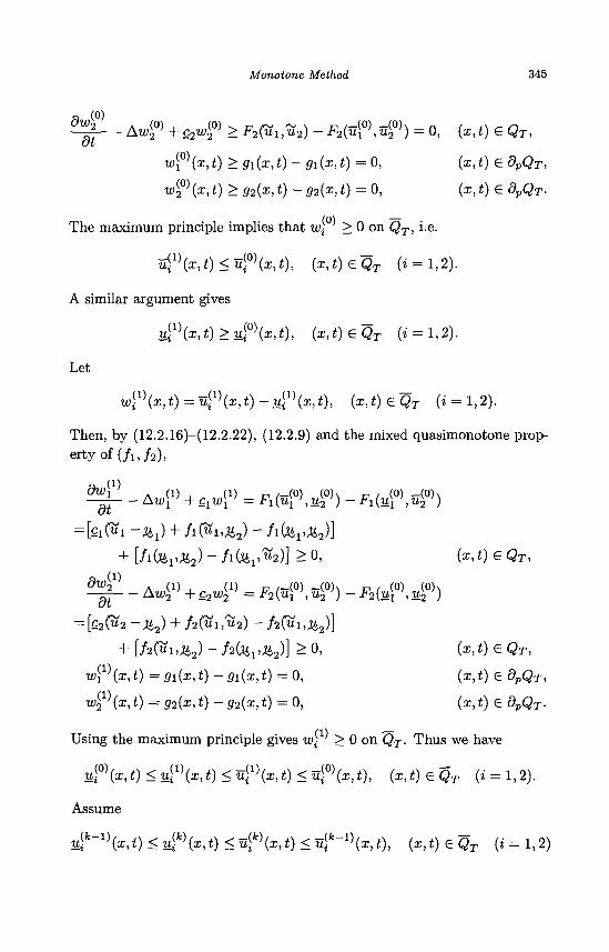
Monotone Method 345
dw{0)
£ - - Aw20) +c2w^ > F2(VUV2) - F2(u?\u2
0)) = 0, (x,t) G Q r , at
u;j0)(a;,*) >Si (a : , i ) - s i (a ; , i ) = 0 , OM) edpQT,
w20)(x,t) > g2(x,t) - g2{x,t) = 0, (x,t) G dpQT.
The maximum principle implies that w\ > 0 on <2T, i.e.
u ^ O M ^ f W ) , (M)eQr (* = l,2).
A similar argument gives
l£\x,t)>di0\x,t), {x,t)eQT (i = 1,2).
Let
wl1)(x,t) = u(.1)(x,t)-v^\x,t), (x,t)eQT (i = 1,2).
Then, by (12.2.16)-(12.2.22), (12.2.9) and the mixed quasimonotone property of ( / i , / 2 ) ,
a (1)
^ - - Au,'1' + clW{1] = i ° U 0 ) ) - f i fcM*) = [ 2 1 ( ^ 1 - ^ ) + / i ( u i > ^ 2 ) - / i ( l 4 1 , ^ 2 ) ]
+ [/i(%!^2) " /i(%!. "2)] > 0, (x,i) G Q r >
^ 2 1 } A,„(i) , „ ,.,(i) _ p (7!(0) (0)v p , (0) (o)s —— Ziw2 +c2u;2 — i'2(u1 ,u2 J—i,
2(,u1 ,u2 )
= [c2(W2 -^42) + f2(ui,U2) - /2(Ul,^2)]
+ [/a(Si,A42)-/2Cl41,«2)] > 0 , (x,t)GQT,
w^\x,t) = gi(x,t) -gi(x,t) = 0, (z,t) G dpQT,
w£\x,t) = g2(x,t) - g2(x,t) = 0, (x,t) G dpQr-
Using the maximum principle gives w\ > 0 on Q T . Thus we have
v!i0\x,t)<y!i1\x,t)<v!i1)(x1t)<v!i0){x,t), (x,t)eQT (t = l ,2).
Assume
^ " ^ ( x . t ) ^ " , - * ^ * . * ) ^ ^ ^ . * ) ^ ^ * " 1 ^ ^ * ) , ( x ,* )GQ T (» = 1,2)
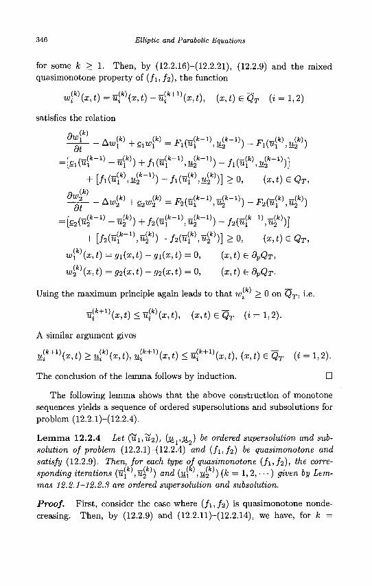
346 Elliptic and Parabolic Equations
for some k > 1. Then, by (12.2.16)-(12.2.21), (12.2.9) and the mixed quasimonotone property of ( / i , /2) , the function
w?\x,t)=u?\x,t)-u?+i\x,t), (x,t)eQT (t = 1,2)
satisfies the relation
a CO
= [c1(uri> -*<*>) + / i ^ . a ? - 1 5 ) - /ip^U*"1*)]
+ [/i(u(1fc),i4fc"1)) - /i(5(ifc),l4fc))] > 0, (x,t) € QT,
a CO ^ - - A«4« + rf = F2{uri\utl)) - F2(rf\&)
=Uutx) - 4fc)) + Mutl)Mtl)) - /adzi*"1', )] + [Mu^M^) - f2(u[k\4k))} > 0, (x,t) e Q T ,
u4fc)(x,t) =ffi(x,t) - 5 i ( x , t ) = 0, (x,i) e dpQT,
w{k\x,t) = g2(x,t) - g2(x,t) = 0, (a:,*) <G dpQT-
Using the maximum principle again leads to that w\ > 0 on QT, i.e.
uf+l\x,t)<uf\x,t), {x,t)£QT (t = l ,2).
A similar argument gives
£+1\x,t) >^k)(x,t),y^k+1\x,t) <u^+1\x,t), (x,t)eQT (. = 1,2).
The conclusion of the lemma follows by induction. D
The following lemma shows that the above construction of monotone sequences yields a sequence of ordered supersolutions and subsolutions for problem (12.2.1)-(12.2.4).
Lemma 12.2.4 Let (u\,U2), (^,,^i2) be ordered supersolution and sub-solution of problem (12.2.1)-(12.2.4) and (A,/2) be quasimonotone and satisfy (12.2.9). Then, for each type of quasimonotone ( / i , /2) , the corresponding iterations (u\ ,u~2 ) and O i >^2 ) (^ = 1,2,• • •) given by Lemmas 12.2.1-12.2.3 are ordered supersolution and subsolution.
Proof. First, consider the case where (/i , /2) is quasimonotone nonde-creasing. Then, by (12.2.9) and (12.2.11)-(12.2.14), we have, for k =
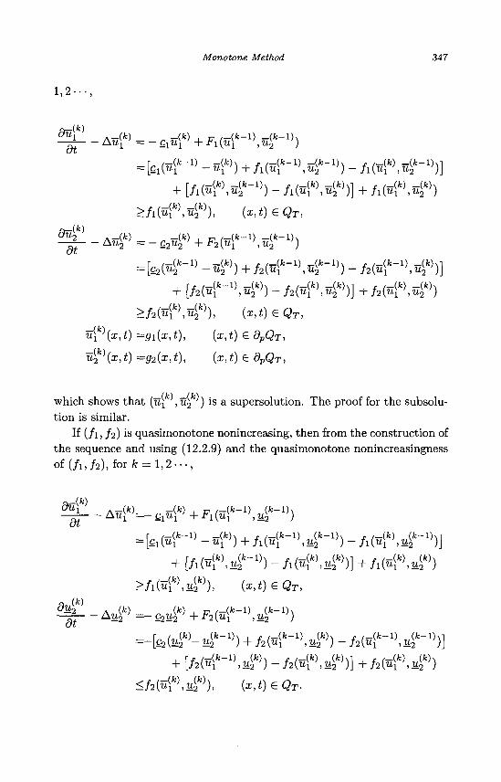
Monotone Method 347
1.2--
-k^*"1 ' - J?) + fM^Mt1') - fMk)Mt1])] + [h(u[k\uri]) - fMk)Ak))] + fMk)Ak))
>h(uf\uik)), (x,t)eQT,
»-(*0
= [fi.(4*-1)-^)) + /3(Bifc-1).4fc-1))-/a(Bi*-1),^))]
>f2{u{k),u(k)), ( i , t ) 6 Q r ,
u^fe)(a;,t) =5i(a;,t), (a:,i) G dpQT,
u(k){x,t) =g2{x,t), (x,t) £ dpQT,
which shows that (u^ , u2 ) is a supersolution. The proof for the subsolu-tion is similar.
If (/i , f2) is quasimonotone nonincreasing, then from the construction of the sequence and using (12.2.9) and the quasimonotone nonincreasingness of ( / i , / 2 ) , for fc = l , 2 . . - ,
-fetfi*-1' --ife)) + h(ut1)Ak~1)) - fMk),i£-l))] + [h(u[k)Ak-1]) - fMk\uik))] + fMk\y^k))
>fi(^k\i^k)), (x,t)eQT,
+ [f2(u[k-l\u2k)) - h(u[k\uik))} + f2(u[k),U2
k))
<f2(u{k),u2k)), (x,t)£QT.
duik)
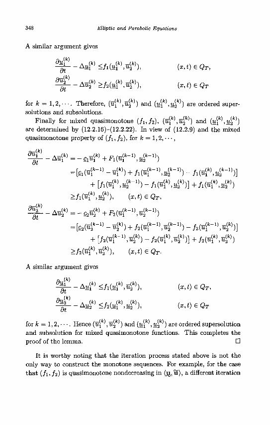
348 Elliptic and Parabolic Equations
A similar argument gives
Ft (fe)
^ - Au[V <fl(u[k\uP), (x,t)€QT,
a—(fc) ^ - Au^ >f2(u[k\4% (x,t)eQT
for k = 1,2, •••. Therefore, (u[ sujj ) and (uf\u2k^) are ordered super-
solutions and subsolutions. Finally for mixed quasimonotone ( / i , /2) , (u\ ,u2 ) a n d (u[ \u2 )
are determined by (12.2.16)-(12.2.22). In view of (12.2.9) and the mixed quasimonotone property of (/i, / 2 ) , for k = 1,2, • • •,
=[a^1fc-i) - + / 1 ( ^ - i ) , ^ - i ) ) - Adtfu*-1')] + [/iti'U*"1') -/ifltfU*')] +h(u[k\u^)
>fi(uf\u^), (x,t)eQT, o-(fe)
^--A^^-c^+^^r1),^-1)) = Uu{tl) ~ 4 f c )) + /a(Bi*-1 ) . '4*-1 )) - f2(u[k-1},uik))]
>f2(u{k),U{2k)), (x,t)£QT.
A similar argument gives
a (*0 ^ - - A«jfc> ^ A ^ , ^ ) , (s , i) e QT ,
^ - Auik) <h(u[k\uik)), (x,t) G Q T
for fc = 1,2, • • •. Hence (uj ,u2 ) and (u^ ,u 2 ) are ordered supersolution and subsolution for mixed quasimonotone functions. This completes the proof of the lemma. •
It is worthy noting that the iteration process stated above is not the only way to construct the monotone sequences. For example, for the case that (/i , A) is quasimonotone nondecreasing in (JJ, u) , a different iteration
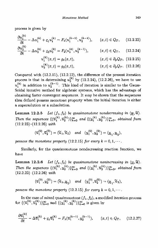
Monotone Method 349
process is given by
a CO ^ - - A u f ' + c ^ f = F^-V^-V), (x,t) G QT, (12.2.23)
a (*) ^ - - A4 f e ) + c24 fc ) = F a ^ , ^ " 1 5 ) , (x,t) G Q r , (12.2.24)
u(1
fe)(x,i) = 5 i ( ^ 0 . (x,t)£dpQT, (12.2.25)
4 f c ) ( x , 0 = 5 2 ( x , t ) , ( x , 0 e 9 p Q r - (12.2.26)
Compared with (12.2.11), (12.2.12), the difference of the present iteration process is that in determining u2 by (12.2.24), (12.2.26), we have to use u[ ' in addition to u2 • This kind of iteration is similar to the Gauss-Seidal iterative method for algebraic systems, which has the advantage of obtaining faster convergent sequences. It may be shown that the sequences thus defined possess monotone property when the initial iteration is either a supersolution or a subsolution.
Lemma 12.2.5 Let ( / i , /2) be quasimonotone nondecreasing in ( j j ,u).
Then the sequences {(u[ ,u2 )}T=o and {(^i '^2 )}V=o> obtained from (12.2.23)-(12.2.26) with
(uf\u20)) = (ui,u2) and (uf\u2
0)) = (MV&2),
possess the monotone property (12.2.15) for every k = 0,1, • • •.
Similarly, for the quasimonotone nondecreasing reaction function, we have
Lemma 12.2.6 Let ( / i , /2) be quasimonotone nonincreasing in ( J J , U ) .
Then the sequences {(u\ ',u2 )}j£L0 and {(u[ ' ,u2 )}'j*L0, obtained from
(12.2.23)-(12.2.26) with
(uf\u20)) = (ui,&2) and {u^ ,u2
0)) = (&vu2),
possess the monotone property (12.2.15) for every k = 0,1, • • •.
In the case of mixed quasimonotone (/i , f2), a modified iteration process
for {(u[k\u2k))}kLo and {(u(
1fc),«3
fc))}2°=0 i s § i v e n hY
^ L _ - Au[V +Qlu[k) = Fi(n (1
f c-1 ) ,4 f e _ 1 )), ( M ) G QT, (12.2.27)
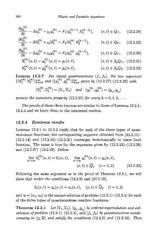
350 Elliptic and Parabolic Equations
ft (fe)
% - - A«ife) + 0 ^ = FM^Mt^), (x,t) € QT, (12.2.28) dt
dtik)
2 - - A u f » + c 2 f = ^ ( S f ' , ^ " 1 ' ) , (x,t) G Q T , (12.2.29) <9*
(fe) du2 ^ A M ^ + C ^ ^ ^ ^ , ^ - 1 ' ) , ( i , t ) 6 Q T l (12.2.30)
u[k)(x,t)=u[k\x,t)=gi(x,t), (x,t)edpQT, (12.2.31)
u ^ O M H u ^ O M ^ ^ f a , * ) . (x,t)edpQT. (12.2.32)
Lemma 12.2.7 For mixed quasimonotone ( / I , / ^ ) , *fee iwo sequences {(u(k),u{
2k))}kLo and {(u[k),w2
fe))}£L0 #wen 6y (12.2.27)-(12.2.32) with
(u{°),u{°)) = {ui,u2) and (ufKuf) = (% i ;u2)
possess the monotone property (12.2.15) for every k = 0,1,2, • • •.
The proofs of these three lemmas are similar to those of Lemmas 12.2.1-12.2.3 and we leave them to the interested readers.
12.2.4 Existence results
Lemmas 12.2.1 to 12.2.3 imply that for each of the three types of quasimonotone functions, the corresponding sequence obtained from (12.2.11)-(12.2.14) and (12.2.16)-(12.2.21) converges monotonically to some limit function. The same is true for the sequences given by (12.2.23)-(12.2.26) and (12.2.27)-(12.2.32). Define
lim u\ (x,t) =Tii(x,t), lim u\ (x,t) = Ui(x,t), fc—>oo fc—*oo
(x,t)eQT (i = 1,2). (12.2.33)
Following the same argument as in the proof of Theorem 12.1.1, we will show that under the conditions (12.2.9) and (12.2.10),
Ui(x,i) = Ui(x,t) = Ui(x,t), (x,t)eQT (i = l,2)
and u = (ui,U2) is the unique solution of problem (12.2.1)-(12.2.4) for each of the three types of quasimonotone reaction functions.
Theorem 12.2.1 Let (ui,'u2), (M,i>Zi,o) ^e ordered supersolution and sub-solution of problem (12.2.1)-(12.2.4), and ( / i , /2) be quasimonotone nonde-creasing in (jj,u) and satisfy the conditions (12.2.9) and (12.2.10). Then
Monotone Method 351
problem (12.2.1)-(12.2.4) has a unique solution u = (1x1,1x2) in ( J J , U ) .
Moreover, the sequences {(u[ ' ,u2 )}fclo and ihA >^2 )}/£o> obtained from (12.2.11)-(12.2.14) with
(u i 0 ) , ^ 0 ) ) = (ui,U2) a ^ ("i0),w20)) = (% i ;^2),
converge monotonically to (ui,u2) and satisfy the relation
(M,v&2) < (uifc),W2fc)) ^ («i»"2) < (uifc),u2fe)) < (u i ,u 2 ) on Q T
(12.2.34) /or every /c = 1, 2, • • •.
Proof. Consider problem (12.2.11)—(12.2.14) where the sequence {u(fc)}£L0 represents either {u{k)}^=0 or {u(fc)}£L0. Since by Lemma 12.2.1 this sequence converges monotonically to some limit (1*1,112) as k —» 00, the continuity and monotonicity property of Fi imply that F(u[ ,u2 ) converges monotonically to Fi{u\,u2) f° r i = 1,2. Prom the regularity of solutions of heat equations,
U(D e ca'a'\QT), ujfc) G C2+a'1+a/2(QT), k = 2,3, • • •
and
\ui \2+a,l+a/2;QT <Ci(\gi\2+a,l+a/2;QT
+ lul'C~1) W,QT + \u2k~l) lo;QT)> & = 2, 3, • • • ,
where i = 1,2, and C» > 0 is a constant depending only on a, fi, T and /i but independent of k. From the monotone property (12.2.15), {«!fc)}EU(* = i . 2 ) is_ uniformly bounded in C 2 + a ' 1 + a / 2 ( Q T ) . Therefore, u e C2+a<1+a/2(QT) is a solution of problem (12.2.1)-(12.2.4). And (12.2.34) follows from the monotone property (12.2.15).
Now we show that
Ui(x,t) =Ui(x,t), (x,t) <=QT (i = 1,2). (12.2.35)
Let
Wi(x,t) =ui(x,t) -Ui(x,t), (x,t)eQT (i = 1,2).
Then, from the monotone property (12.2.15),
Wi(x,t)<0, (x,t) £QT (i = 1,2). (12.2.36)
352 Elliptic and Parabolic Equations
By_(12.2.1)-(12.2.4) and the condition (12.2.10), Wi € C2<l{QT) n C(QT) (i = 1,2) satisfies
- ^ - Awi =fi(ul,u2) - fi{ui,u2)
>Ci((«i -iLi) + (u2 -M2)) = -c%{wi + w2), (x,t) € QT,
Wi(x,t) =gi(x,t) -gi(x,t) = 0 , (x,t) e dpQT.
Therefore, w\ + u>2 satisfies the relation
&t ~ A ^ x +W2) ~ ~ (5i + 5 2 ) ( ^ i + ^2), (x,t) e QT,
(WI + w2)(x, t) =0, (x, t) G dpQT-
The maximum principle guarantees that
wi(x,t) + W2(x,t) > 0, (x,t)£QT.
This and (12.2.36) lead to (12.2.35). Prom (12.2.35), to show the uniqueness of the solution of problem
(12.2.1)-(12.2.4) in (ji, u) , it suffices to verify that any solution u* S (JJ, u) to problem (12.2.1)-(12.2.4) satisfies the relation
u(x,t) <u*(x,t) <u(x,t), (x,t) € QT.
This may be proved by the same argument as in the proof of Theorem 12.1.1 ii) and we leave the details to the reader. •
For the other two types of quasimonotone reaction functions, we may prove similarly the following theorems.
Theorem 12.2.2 Let ( w i , ^ ) , (%j,^i2) be ordered supersolution and sub-solution of problem (12.2.1)-(12.2.4), and (fi,fa) be quasimonotone nonin-creasing in (JJ,U) and satisfy the conditions (12.2.9) and (12.2.10). Then problem (12.2.1)-(12.2.4) has a unique solution u = (ui,U2) in ( j j ,u) .
Moreover, the sequences {(u[ ',u2 ) } ^ 0 and (C^i »*4 )}fcio> obtained
from (12.2.11)-(12.2.14) with
(w(i0),u20)) = (u i ,^ 2 ) and (u^ ,u2
0)) = (%vu2),
converge monotonically to (u\,u2) and satisfy the relation (12.2.34).
Theorem 12.2.3 Let (ui,U2), (%i;,%2) be ordered supersolution and sub-solution of problem (12.2.1)-(12.2.4), and ( / i , /^) be quasimonotone nonin-creasing in (JJ,U) and satisfy the conditions (12.2.9) and (12.2.10). Then
Monotone Method 353
problem (12.2.1)-(12.2.4) has a unique solution u — (1x1,112) in ( J J , U ) .
Moreover, the sequences {(u[ ,u2 )}feLo and {(^1 '—2 )}j£=o> obtained from (12.2.16)-(12.2.21) with
(uf} ,u{2]) = (u!,u2) and {uf\u20)) = (&v&2),
converge monotonically to (ui,u2) and satisfy the relation (12.2.34).
When the iteration processes (12.2.11)-(12.2.14) and (12.2.16)-(12.2.21) are replaced by (12.2.23)-(12.2.26) and (12.2.27)-(12.2.32), respectively, the results of Lemmas 12.2.5 to 12.2.7 imply that the corresponding sequences converge to some limit functions in the same fashion as in (12.2.33). It is easy to prove by an argument similar to the proof of Theorems 12.2.1 to 12.2.3 that these limits are also solutions of problem (12.2.1)-(12.2.4) in accordance with the quasimonotone property of ( / i , /2) . This observation leads to the following conclusion.
Theorem 12.2.4 Under the hypothesis of Theorems 12.2.1-12.2.3, except that the iteration processes (12.2.11)-(12.2.14) and (12.2.16)-(12.2.21) are replaced by (12.2.23)-(12.2.26) and (12.2.27)-(12.2.32) respectively, all conclusions in the corresponding theorem remain true.
12.2.5 Extension
As the scalar equations, the monotone method used above may be applied to coupled uniformly parabolic systems of general form with more general reaction terms, such as the system
r\ n n
-W - E afffaQDjUn + Y/bf)(x,t)Dju1 j,i=i j=i
+ c(-1\x,t)u1 = fi(x,t,ui,u2), (x,t) G QT,
^-J2 afi^D^ + j^bfix^D^ 3,1=1 j=i
+ c{2)(x,t)u2 = h{x,t,uuu2), (x,t) G QT,
ui(x,t) = gi(x,t), (x,t)edpQT,
u2(x, t) = g2(x, t), (x, t) G dpQT,
where fl C Rn is a bounded domain with dCl G C2,a for some 0 < a < 1, / . G Ca,a/2,a(QT x R 2 ) | g. g cS+a.l+a/a^), a« )6«>cM g Q^a/2^^
354 Elliptic and Parabolic Equations
ajl = aij a n d there exist positive constants A^ , A ^ , such that
A ( % | 2 < £ «!?(*>*&& < A ^ i a 2 , V£ e R", (x,t) g Q T
for each i = 1,2. At the end of this section, we point out that the monotone method
may be used to coupled elliptic systems and also to parabolic and elliptic systems with an arbitrary finite number of equations, see more details in [Pao (1992)].
Exercises
1. Prove Remarks 12.1.1 and 12.1.2. 2. Prove Lemmas 12.2.5-12.2.7. 3. Prove Theorems 12.2.2-12.2.4. 4. Apply the monotone method to general coupled uniformly parabolic
systems. 5. Apply the monotone method to elliptic equations and coupled sys
tems. 6. Establish the theory of monotone method for elliptic and parabolic
systems with an arbitrary finite number of equations.
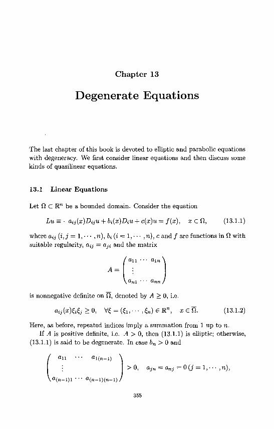
Chapter 13
Degenerate Equations
The last chapter of this book is devoted to elliptic and parabolic equations with degeneracy. We first consider linear equations and then discuss some kinds of quasilinear equations.
13.1 Linear Equations
Let ft c i n be a bounded domain. Consider the equation
Lu = — aij(x)DijU + bi(x)DiU + c(x)u = f(x), x G fl, (13.1.1)
where a^ (i,j = 1, • • • , n), bi (i = 1,- • • , n), cand / are functions in Q with suitable regularity, a - = a,ji and the matrix
( a n ••• air,
Ojn\ ' ' ' Qjir
is nonnegative definite on Q, denoted by A > 0, i.e.
M a : ) & & > 0 , V£ = (£i, ••• ,£«)€]&", xGf t . (13.1.2)
Here, as before, repeated indices imply a summation from 1 up to n. If A is positive definite, i.e. A > 0, then (13.1.1) is elliptic; otherwise,
(13.1.1) is said to be degenerate. In case bn > 0 and
/ a n ••• ai(n-i) \
: > 0, ajn = anj = 0 (j = 1, • • • , n),
\ a ( n - l ) l ••• a ( n - l ) ( n - l ) /
355
356 Elliptic and Parabolic Equations
(13.1.1) is a parabolic equation; this means that, parabolic equations are degenerate elliptic equations. If bn > 0 and
f an ••• ai(„_i) \
: > 0 , ajn =an}=0(j = l,--- ,n) ,
\ 0 ( n - l ) l ••• a ( n - l ) ( n - l ) /
then (13.1.1) is a degenerate parabolic equation. If
a n • • • o-im ^
: > 0 , 0 < m < n - 2 ,
^ ^ m l ' ' ' Q"m7n /
a-ij = dji = 0 (i = m + I, • • • , n; j = 1, • • • , n ) ,
then (13.1.1) is called an ultraparabolic equation. In the extreme case dij = 0 (i, j = 1, • • • , n), (13.1.1) degenerates into a first order equation.
Sometimes, it is convenient to write (13.1.1) in divergence form
Lu = -Dj(aij(x)Diu) + /3i(x)DiU + c{x)u = f(x), x G Q (13.1.3)
where
Pi(x) = bi(x) + Dj<iij(x), x e fi (i = l, • • • , « ) .
13.1.1 Formulation of the first boundary value problem
Different from elliptic equations without degeneracy, to pose the first boundary value problem for degenerate elliptic equations, in general, we are not permitted to prescribe the boundary value on the whole boundary
Suppose that £ = dCl is piecewise smooth. Denote
E° = {x £ H;aij(x)vi{x)vj(x) = 0}
and
(3(x) = j3i(x)ui(x), x€E,
where V = (v\, • • • , un) is the unit normal vector inward to E; 0(x) is called the Fichera function. Divide S° as follows
S° = E0 U Si U E2
Degenerate Equations 357
and denote
where
Then
E3 = S\E°,
S 0 = { x e E 0 ; / 3 ( x ) = 0 } ,
Ei = {x£ Z°;P(x) < 0 } ,
£ 2 = { x e E ° ; / ? ( x ) > 0 } .
E3 = {x G E;aij(o;)^(1)^(3;) > 0 } U J E ,
where £ is a possible subset of measure zero on E. Since E = 60, is piecewise smooth, there might be a subset of measure zero on E, at any point of which, no normal exists.
The first boundary value problem for (13.1.1) or (13.1.3) is then formulated as follows
Lu = / , i £ ( l , (13.1.4)
u =g, (13.1.5) s2us3
where g is a given function. Let us observe some special examples. If (13.1.1) is elliptic, then E° is an empty set, E = E3 and we need to
prescribe the boundary value on the whole boundary E. For equations of the form
Lu = —Dj(a,ijDiu) + c(x)u = f(x), x G fi, (13.1.6)
we have f3(x) = 0, Eo = E° and E2 is empty. Thus only the boundary value on E3 needs to be given.
Now we consider the parabolic equation
du — - a,ij(x,t)DijU + bi(x,t)DiU + c(x,t)u = f(x,t),
( i , t ) e Q T = ftx(0,T), (13.1.7)
where oy (i,j = 1, • • • ,n) , 6» (i — 1, • • • ,n) , c and / are functions on QT
with suitable regularity and atj = a^ satisfy the condition
O i j & ^ > 0 , £ = ( £ i , - - - , € n ) € R n , £ ^ 0 , (x,t)eQT. (13.1.8)
358 Elliptic and Parabolic Equations
Denote t = xn+1, a{n+1)i = a i ( n + i ) = 0(i = 1,- • • ,n + 1), bn+1 = 1. Then (13.1.7) can be expressed as (13.1.1) or (13.1.3) with i,j = 1, • • • ,n + 1, x = (xi, • • • ,xn,xn+i) and fi x (0,T) in place of Q. In the present case,
£ = d Q r = ( f lx{« = xn+1 = 0}) U (n x {t = arn+1 = T}) U (Sfi x (0,T))
and the Fichera function is
n+l n
P = ^PiVi = Y^PM + "n+l-» = 1 t = l
n+l On the lower bottom ft x {t = x n + i = 0}, we have VJ a^ViVj = 0,
/3 = 1 > 0 and hence Q x {i = x n + 1 = 0} C E2, where the boundary value needs to be given. However, on the upper bottom CI x {t = xn+i = T}, n+l 2_] CLijVii/j = 0, /? = —1 < 0, which means that Ct x {t = xn+i = T} C Si ,
»,j=i where we should not give the boundary value. Since oy satisfy (13.1.8),
n+l n on the lateral boundary dVt x (0,T), Y^ a^ViVj = VJ a^ViVj > 0, i.e.
dfl x (0, T) = E3, where the boundary value needs to be given. Prescribing the boundary value on the lower bottom and the lateral boundary is just the usual formulation of the first boundary value problem for parabolic equations.
It is natural to ask why we formulate the first boundary value problem for (13.1.1) in the above manner. The basic idea is to search such a boundary value condition which can ensure the uniqueness and existence of the solution. A proper condition should first ensure that the homogeneous equation has only zero solution satisfying the homogeneous boundary value condition.
Let us first consider the special equation (13.1.6). Suppose that u £ C2(Q) is a solution of
Lu=~Dj(aijDiu) + cu = 0, (13.1.9)
satisfying the homogeneous boundary value condition. Multiply both sides of (13.1.9) by u and integrate over O. After integrating by parts we obtain
0 = / uLudx = — / uDj(a,ijDiu)dx + / cu2dx Jn Jn Jn
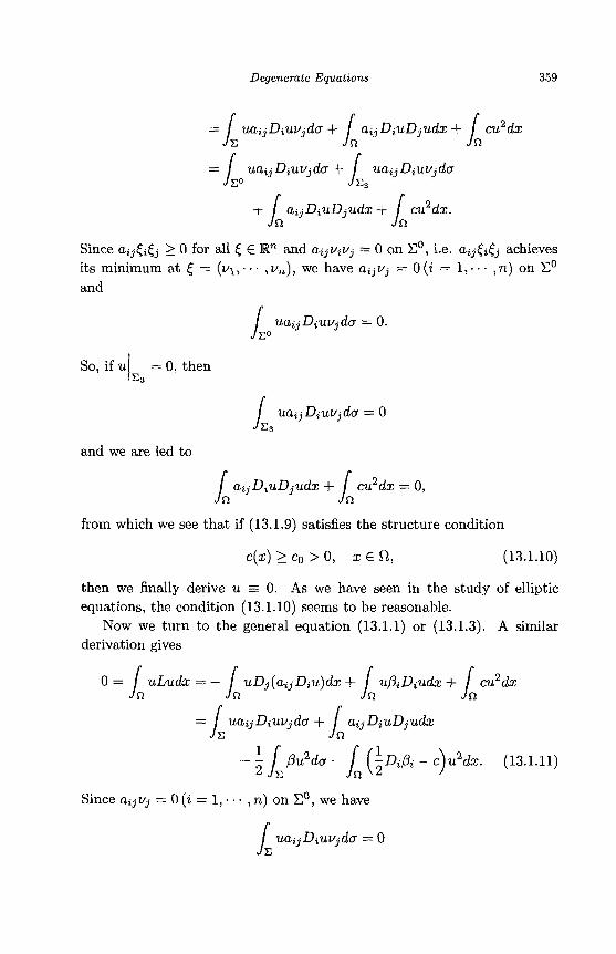
Degenerate Equations 359
= / uaijDiUVjda + / aijDiuDjudx+ / cu2dx JT, JQ JQ
= I uaijDiUUjda + j uaijDiUVjda JT,0 JT3
+ [a,DiuDjudx+[cu>dX. JQ JQ
Since ay£»£j > 0 for all £ e R" and dijViVj = 0 on S°, i.e. ay£j£j achieves its minimum at f = (i/i, • • • , fn)> we have ajji/j = 0 (i = 1, • • • ,n) on S° and
/ udijDiUVj JT°
ida = 0.
So, if u = 0, then s 3
/ uaijD JT,3
iUVjda = 0
and we are led to
/ dijDiiiDjudx + / cu2dx — 0, JQ JQ
from which we see that if (13.1.9) satisfies the structure condition
c(x) > Co > 0, x £ n, (13.1.10)
then we finally derive u = 0. As we have seen in the study of elliptic equations, the condition (13.1.10) seems to be reasonable.
Now we turn to the general equation (13.1.1) or (13.1.3). A similar derivation gives
0 = / uLudx — — J uDj(dijDiu)dx + / u[liDiudx+ j cu2dx JQ JQ JQ JQ
= I uaijDiUVjda + I dijDiuDjudx JT, JQ
- 1 j j3u2da - / ( 5 A A ~ c^u2dx. (13.1.11)
Since dijVj = 0 (i = 1, • • • , n) on E°, we have
/ UdijDiUVj da = 0 JT,
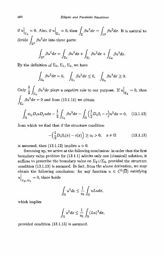
360 Elliptic and Parabolic Equations
if = 0. Also, if u s3
= 0, then / f3u2da = I /3u2da. It is natural to s3 JY. JYP
= 0, then s2
[ (3u2da = f
divide / Pu2da into three parts JT,0
/ pv?d(T = / f3u2dx + / /3u2dx + [ Pu2dx. Jn° JEo VSi Js2
By the definition of E0, £1 , £2, we have
I (3u2da = 0, / (3u2da < 0, f (3u2da > 0. JSo J S I «/S2
Only - / (3u2da plays a negative role to our purpose. If * i s 2
/ j3u2dcr = 0 and from (13.1.11) we obtain JT.2
\ aijDiuDjudx - - / (3u2da - I (-Dif3i-c)u2dx = 0, (13.1.12)
from which we find that if the structure condition
- (^Di0i(x) - c(x)) > co > 0, x e J2 (13.1.13)
is assumed, then (13.1.12) implies u = 0. Summing up, we arrive at the following conclusion: in order that the first
boundary value problem for (13.1.1) admits only one (classical) solution, it suffices to prescribe the boundary value on £ 2 U £3, provided the structure condition (13.1.13) is assumed. In fact, from the above derivation, we may obtain the following conclusion: for any function u e C2(Cl) satisfying
u — 0, there holds E2US3
/ u2dx < — / uLudx, Jn °o Jn
which implies
/ u2dx <— (Lu)2dx, Jn °o Jn
provided condition (13.1.13) is assumed.
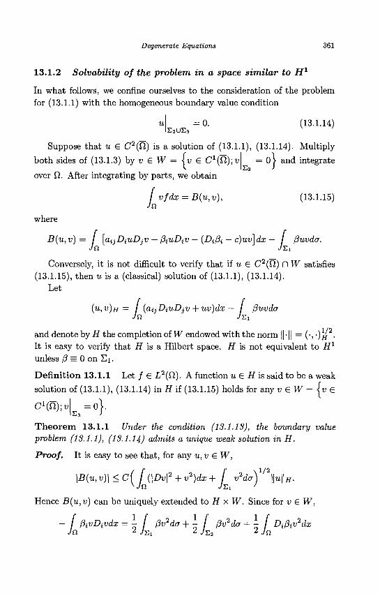
Degenerate Equations 361
13.1.2 Solvability of the problem in a space similar to H1
In what follows, we confine ourselves to the consideration of the problem for (13.1.1) with the homogeneous boundary value condition
= 0. (13.1.14) E 2US 3
Suppose that u G C2(U) is a solution of (13.1.1), (13.1.14). Multiply
both sides of (13.1.3) by v £ W = \v £ C 1 ^ ) ^ = 0 ) and integrate
over fi. After integrating by parts, we obtain
L vfdx = B(u,v), (13.1.15)
where
B{u,v) = / [aijDiuDjV — piuDiV — (Di/3i — c)uv\dx — I (3uvda.
Conversely, it is not difficult to verify that if u G C2(0) (~l W satisfies (13.1.15), then u is a (classical) solution of (13.1.1), (13.1.14).
Let
(U,V)H = / (aijDiuDjV+ uv)dx — / fiuvda
and denote by H the completion of W endowed with the norm |HI = ( V ) H • It is easy to verify that if is a Hilbert space. H is not equivalent to H1
unless 0 = 0 on S i .
Definition 13.1.1 Let / € L2(0). A function u € H is said to be a weak
solution of (13.1.1), (13.1.14) in H if (13.1.15) holds for any v £ W = iv £
C^U^v = 0 ) .
Theorem 13.1.1 Under the condition (13.1.13), the boundary value problem (13.1.1), (13.1.14) admits a unique weak solution in H.
Proof. It is easy to see that, for any u, v € W,
\B(u,v)\<c(^(\Dv\> + v>)dx + ^ v*do-)1/2 \\U\\H-
Hence B(u, v) can be uniquely extended to H x W. Since for v € W,
- / PivDivdx = - / f3v2da + - (3v2da +- D^v^dx
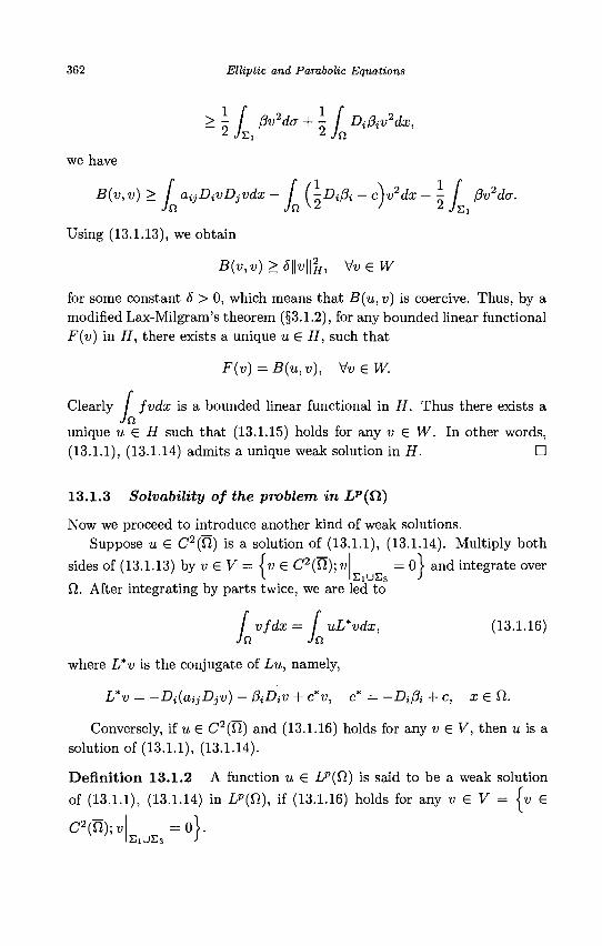
362 Elliptic and Parabolic Equations
>]-[ (3v2da + i f DipiV2dx,
have
B(v,v)> / aijDivDjvdx- / (-Di/3i-c)v2dx-- / pv2da. J a Jny* ' 2 •/£!
Using (13.1.13), we obtain
B(v,v)>S\\v\\2H, V v e W
for some constant 5 > 0, which means that B(u,v) is coercive. Thus, by a modified Lax-Milgram's theorem (§3.1.2), for any bounded linear functional F(v) in H, there exists a unique u £ H, such that
F(v) = B{u,v), VveW.
Clearly / fvdx is a bounded linear functional in H. Thus there exists a
unique u G H such that (13.1.15) holds for any v € W. In other words, (13.1.1), (13.1.14) admits a unique weak solution in H. O
13.1.3 Solvability of the problem in Lp(Ct)
Now we proceed to introduce another kind of weak solutions.
Suppose u G C2(fi) is a solution of (13.1.1), (13.1.14). Multiply both
sides of (13.1.13) by v G V = \v G C2(fi); v = 0 j and integrate over
O. After integrating by parts twice, we are led to
/ vfdx = I uL*vdx, (13.1.16) Jn Jn
where L*v is the conjugate of Lu, namely,
L*v = -Di(a,ijDjv) - PiDiV + c*v, c* = - A A +c, x G 0 .
Conversely, if u G C2(Vt) and (13.1.16) holds for any v £V, then u is a solution of (13.1.1), (13.1.14).
Definition 13.1.2 A function u G LP(Q) is said to be a weak solution
of (13.1.1), (13.1.14) in Lp(ft), if (13.1.16) holds for any v G V = iv G
c2(ay,v =o\.
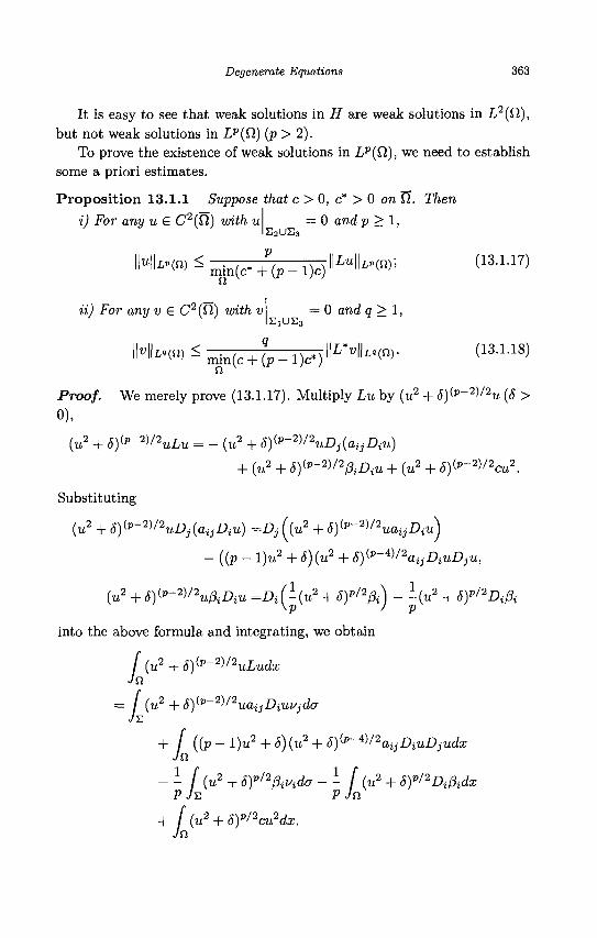
Degenerate Equations 363
It is easy to see that weak solutions in H are weak solutions in L2(£l), but not weak solutions in Lv{0) (p > 2).
To prove the existence of weak solutions in LP(Q,), we need to establish some a priori estimates.
Proposition 13.1.1 Suppose that c > 0, c* > 0 on fi. Then
= 0 and p > 1, s2us3
i) For any u £ C2(Q) with u
" M » ^ ^ ^ m i n ( ^ ; ( P - i ) c ) " L u i i ^ ; <i3-u?>
ii) For any v £ C2(Q.) with v = 0 and q>l, E1UE3
IMlL.(n) < • , J , 7^dL*v\\L,m. (13.1.18) K ' min(c+ (p — l)c*) v '
Proof. We merely prove (13.1.17). Multiply Lu by (u2 + S^'^^u (S >
0),
(u2 + S)^-2^2uLu = -(u2 + S^-WuDjiayDiu)
+ (u2 + S^-W&DiU + (u2 + 5)^-2^'2cu2.
Substituting
(u2 + S^WuDjfajDiu) =Di ((u2 + <5)(p~2)/2uay £ \« )
- ((p - l)u2 + 5){u2 + S^WoijDiuDjU,
(u2 + S^-Wu&DiU =DJ-(u2 + 5)*'2fr) - -{u2 + Sy^DiPi \p ) p
into the above formula and integrating, we obtain
/ (u2 + 6)ip~2)/2uLudx JQ
= I (u2 + S^-V^uaijDiUVjda
[ ((p - l)u2 + <5)(u2 + S^-V^aijDiiiDjudx JQ
- - f(u2 + 5)P/2piPida - - f\u2 + SY^DiPidx
+ I(u2 + 5)P'2cu2dx. JQ
+
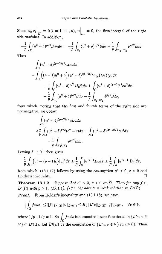
364 Elliptic and Parabolic Equations
Since a^Vj = 0 (i = 1, • • • , n), u ^ = 0 , the first integral of the right
side vanishes. In addition,
P
Thus
- f(u2 + SfVpiVido = - - ( {u2 + 5)p'20du - - f 5p>2pda. V */E r JTi\ P JS2UE3
[ (u2 + 6)(p-2)/2uLudx Jn
= I ((p - l)u2 + j ) (u2 + J) ( p-4 ) / 2ayDiuDjudx
- - f(u2 + 6)^2Dipidx+ f(u2 + 8)^-2V2cu2dx P Jn Jn
- - [ (u2 + 8)p'2j3da - - f 8p'2pda,
from which, noting that the first and fourth terms of the right side are nonnegative, we obtain
/ (u2 + 5){p-2)/2uLudx Jn
>- [(u2 + 6)P/2(c*-c)dx+ [(u2 + 5)(p-2V2ciL2dx P Jn Jn
- - f 6p'2f3do-. P ^S 2 UE 3
Letting 6 —> 0+ then gives
- f (c* + (p - l)c)\u\pdx < - [ \u\p-lLudx <- [ luF^lLuldx, P Jn ^ J PJn pJn
from which, (13.1.17) follows by using the assumption c* > 0, c > 0 and Holder's inequality. •
Theorem 13.1.2 Suppose that c* > 0, c > 0 on fi. Then for any f G LP(Q) withp > 1, (13.1.1), (13.1.14) admits a weak solution in LP(Q).
Proof. Prom Holder's inequality and (13.1.18), we have
/ fvdx < ||/||LP(n)ll«l|L«(n) < Kq\\L*v\\Lgm\\f\\LPm, W G V, Jn
where 1/p+l/q = 1. So / fvdx is a bounded linear functional in {L*v; v G in
V} C Lq(Cl). Let Lq{Q) be the completion of {L*v;v G V} in L«(ft). Then
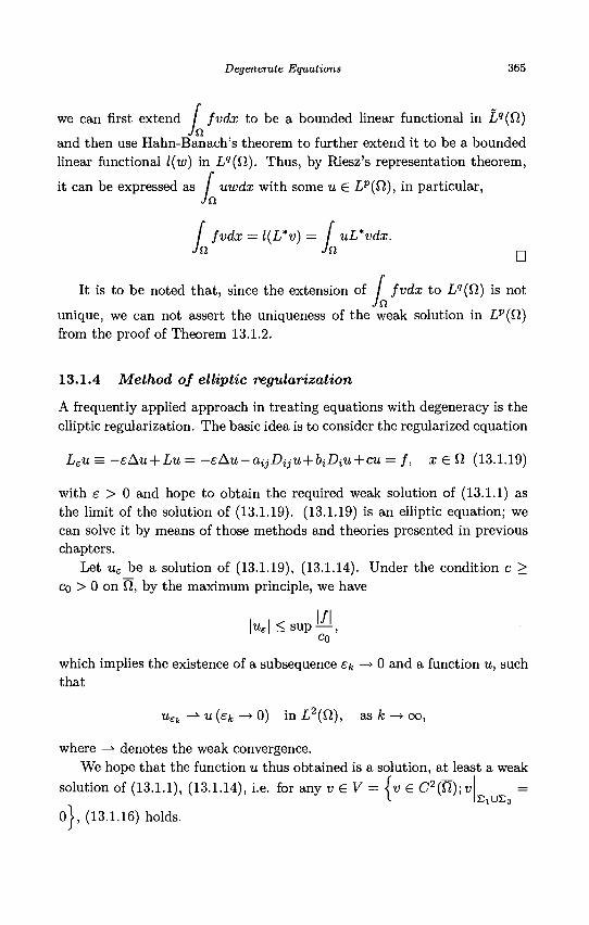
Degenerate Equations 365
we can first extend / fvdx to be a bounded linear functional in Lq(Q.)
and then use Hahn-Banach's theorem to further extend it to be a bounded linear functional l(w) in Lq(Q,). Thus, by Riesz's representation theorem,
it can be expressed as / uwdx with some u € Lp(Cl), in particular, Ja
/ fvdx = l(L*v) = / uL*vdx.
It is to be noted that, since the extension of / fvdx to Lq(Cl) is not Ju
unique, we can not assert the uniqueness of the weak solution in Lp(Cl) from the proof of Theorem 13.1.2.
13.1.4 Method of elliptic regularization
A frequently applied approach in treating equations with degeneracy is the elliptic regularization. The basic idea is to consider the regularized equation
Leu = —eAu + Lu = —eAu — aijDijU + biDiu + cu = f, xGfl (13.1.19)
with e > 0 and hope to obtain the required weak solution of (13.1.1) as the limit of the solution of (13.1.19). (13.1.19) is an elliptic equation; we can solve it by means of those methods and theories presented in previous chapters.
Let ue be a solution of (13.1.19), (13.1.14). Under the condition c > Co > 0 on il, by the maximum principle, we have
l/l \ue\ < sup — , CO
which implies the existence of a subsequence £fc —» 0 and a function u, such that
u£k —^ u (£fc —» 0) in L2(fi), as k —> oo,
where —*• denotes the weak convergence. We hope that the function u thus obtained is a solution, at least a weak
solution of (13.1.1), (13.1.14), i.e. for any v G V = \v € C2(U);v I S1US3
0} , (13.1.16) holds.
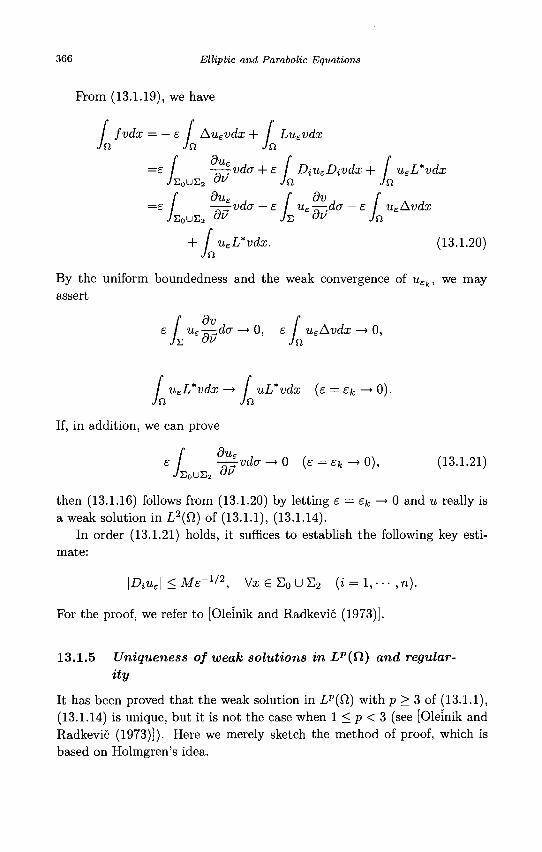
366 Elliptic and Parabolic Equations
Prom (13.1.19), we have
/ fvdx = — e Au£vdx + / Luevdx Ja Jn Jn
=e / -—^vda + e / DiU£Divdx + / ueL*vdx JE0UI;2 VV Jn Jn
f 9uE , f dv , f A , =£ / -^zrvda — e / u£-—acr —£ / ueAvdx
JE 0 UE 2 W J E W Jn
+ / ueL*vdx. (13.1.20) Jn
By the uniform boundedness and the weak convergence of uEk, we may assert
e / u£-—da —> 0, £ / u£Au<ir —> 0,
/ ueL*vdx —> / uL*vdx (£ = ££ —> 0). Jn Jn
If, in addition, we can prove
£ / - ^ v d c r ^ O (e = e f c->0), (13.1.21) JE 0 UE 2 " "
then (13.1.16) follows from (13.1.20) by letting £ = ££ —> 0 and u really is a weak solution in L2(0) of (13.1.1), (13.1.14).
In order (13.1.21) holds, it suffices to establish the following key estimate:
\Dtue\ < M£~1/2, Vx e S 0 U S 2 (i = l,---,n).
For the proof, we refer to [Oleinik and Radkevic (1973)].
13.1.5 Uniqueness of weak solutions in Lp(ft) and regularity
It has been proved that the weak solution in Lp(Cl) with p > 3 of (13.1.1), (13.1.14) is unique, but it is not the case when 1 < p < 3 (see [Oleinik and Radkevic (1973)]). Here we merely sketch the method of proof, which is based on Holmgren's idea.
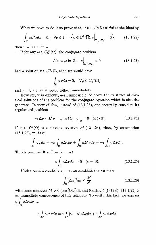
Degenerate Equations 367
What we have to do is to prove that, if u £ LP(Q.) satisfies the identity
uL*vdx = 0, \/veV= (weC 2 ( f l ) ; « = o ) , (13.1.22) L E i U E s >
J Jn in
then u = 0 a.e. in 0 . If for any tp € C^{Q), the conjugate problem
L*v = pmQ, v = 0 (13.1.23) EiUE3
had a solution v € C2(Cl), then we would have
uipdx = 0, Vv? e C^°(Q) / Jn in
and u = 0 a.e. in Q would follow immediately. However, it is difficult, even impossible, to prove the existence of clas
sical solutions of the problem for the conjugate equation which is also degenerate. In view of this, instead of (13.1.23), one naturally considers its regularized problem
-eAv + L*v = ip in Q, v = 0 (e > 0). (13.1.24)
If v G C2(fi) is a classical solution of (13.1.24), then, by assumption (13.1.22), we have
/ wpdx = — s / uAvdx + / uL*vdx = —e uAvdx. Jn Jn Jn Jn
To our purpose, it suffices to prove
e / uAvdx -» 0 (e -> 0). (13.1.25) Jn
Under certain conditions, one can establish the estimate
/ Jn
(Avfdx < ^ (13.1.26) n £
with some constant M > 0 (see [Oleinik and Radkevic (1973)]). (13.1.25) is an immediate consequence of this estimate. To verify this fact, we express
e / uAvdx as Jn
e / uAvdx = e / (u — u')Avdx + e \ u'Avdx Jn Jn Jn

368 Elliptic and Parabolic Equations
= e (u - u')Avdx + £ Au'vdx, Jn Jn
where u' G CQ°(Q,). For any given 5 > 0, using (13.1.26), we may choose
u' G CQ°(Q) such that (u — u')2dx is so small to make Jn
f (u - u')Avdx\ < e ( / (u - u')2rfo;)1/2( /" (Au)2dz) 1/2 J
<2-
For fixed u', using the uniform boundedness of v in e (following from the maximum principle), we have
Jn s I Au'vdx
< 2 '
when e > 0 is small enough. Another important problem for degenerate equations is the regularity
of weak solutions. Many authors have studied the global regularity of weak solutions by means of elliptic regularization. Uniform estimates in Ck(Q) of solutions {ue} of the regularized problems have been established under certain conditions. Based on these estimates, weak solutions of the original problem are proved to be functions in Cfc(fi). Also uniform estimates in some Sobolev space have been established under certain conditions and hence weak solutions are proved to be functions in this space.
The study of local regularity is related to the subellipticity of equations. A linear differential operator with C°° coefficients defined in il is said to be a subelliptic operator, if for any distribution u and any domain ff CC Q, Pu £ C°°(0') implies u G C°°(Q').
It has been proved that any subelliptic operator possesses nonnegative or nonpositive characteristic form. Various conditions have been discovered for linear degenerate elliptic equations of second order to be subelliptic.
13.2 A Class of Special Quasilinear Degenerate Parabolic Equations — Filtration Equations
In this section, we proceed to discuss quasilinear equations. As seen in the previous section, the study of linear degenerate elliptic equations is more difficult than that for equations without degeneracy. Much more difficulty would be caused by the quasilinearity of equations. We do not attempt to present the argument for general degenerate elliptic equations. We merely
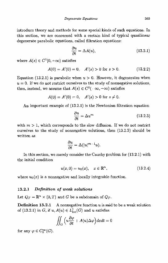
Degenerate Equations 369
introduce theory and methods for some special kinds of such equations. In this section, we are concerned with a certain kind of typical quasilinear degenerate parabolic equations, called filtration equations:
^ = AA(u), (13.2.1)
where A(s) G C1[0,+00) satisfies
A(0) = A'(0) = 0, A'(s) > 0 for s > 0. (13.2.2)
Equation (13.2.1) is parabolic when u > 0. However, it degenerates when u = 0. If we do not restrict ourselves to the study of nonnegative solutions, then, instead, we assume that A(s) E C1(—00, +00) satisfies
A(0) = A'(0) = 0, A'(s) > 0 for s ^ 0.
An important example of (13.2.1) is the Newtonian filtration equation
^ - Aum (13.2.3)
with m > 1, which corresponds to the slow diffusion. If we do not restrict ourselves to the study of nonnegative solutions, then (13.2.3) should be written as
^ = Aw-1!*). In this section, we merely consider the Cauchy problem for (13.2.1) with
the initial condition
U(X,0) = UQ(X), x£Rn, (13.2.4)
where 110(2;) is a nonnegative and locally integrable function.
13.2.1 Definition of weak solutions
Let QT = Mn x (0, T) and G be a subdomain of QT.
Definition 13.2.1 A nonnegative function u is said to be a weak solution of (13.2.1) in G, iiu,A(u) G Lloc(G) and u satisfies
[J (u^ + A(u)A<p)dxdt = 0
for any <p € C%°{G).
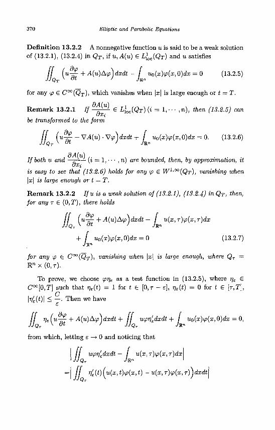
370 Elliptic and Parabolic Equations
Definition 13.2.2 A nonnegative function u is said to be a weak solution of (13.2.1), (13.2.4) in QT, if u, A(u) € L\oc{QT) and u satisfies
/ / (u-£+A(u)&<p)dxdt+ uo(x)(p(x,0)dx = 0 (13.2.5)
for any (p e C°°(QT), which vanishes when |x| is large enough or t = T.
dA(u) Remark 13.2.1 If v J 6 L\oc(QT) (i = 1, • • • ,n), then (13.2.5) can
OXi be transformed to the form
/ / (u-£-VA(u)-V<p)dxdt+ uo(x)<p(x,0)dx = 0. (13.2.6) JJQT ^ °^ ' JVLn
8A(u) If both u and —r (i = 1, • • • , n) are bounded, then, by approximation, it
OXi
is easy to see that (13.2.6) holds for any <p € W1,00(QT), vanishing when \x\ is large enough ort = T.
Remark 13.2.2 Ifu is a weak solution of (13.2.1), (13.2.4) «n QT, then, for any r S (0, T), there holds
\\ ( U 7T "*" A(u)Aip)dxdt — / u(x,r)</?(x,r)dx
+ / u0(x)ip(x,0)dx = 0 (13.2.7)
for any <p S C°°{QT), vanishing when \x\ is large enough, where QT — Rn x (0,r) .
To prove, we choose <pr]e as a test function in (13.2.5), where rje G C°°[0,T] such that rjs(t) = 1 for t € [0,r - e], rjE(t) = 0 for t e [T,T],
(j |J?E(0I — — • Then we have
If r)e(u^+A(u)A<pyxdt+ (J u(pt]'edxdt + J uo(x)tp(x, 0)dx — 0,
from which, letting e —* 0 and noticing that
/ / u(prj'£dxdt — / u(x,T)(fi(x,T)dx JJQT JRn
/ / ^eWf^C^iOvC1)*) — u(x,T)ip(x,T))dxdt
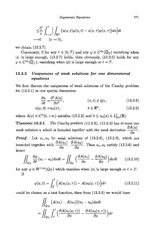
Degenerate Equations 371
<— / / (u(x,t)<f(x, t) — u(x, r)ip(x, r))dx £ Jr-e JRn
—0 (e -> 0),
dt
we obtain (13.2.7). Conversely, if for any r £ (0,T) and any <p £ C°°(QT) vanishing when
\x\ is large enough, (13.2.7) holds, then obviously, (13.2.5) holds for any ip £ C°°(QT), vanishing when \x\ is large enough or t = T.
13.2.2 Uniqueness of weak solutions for one dimensional equations
We first discuss the uniqueness of weak solutions of the Cauchy problem for (13.2.1) in one spatial dimension:
u(x,0) =u0(x), xeRn, (13.2.9)
where A(s) £ C ^ + o o ) satisfies (13.2.2) and 0 < u0{x) £ Lloc(R).
Theorem 13.2.1 The Cauchy problem (13.2.8), (13.2.9) has at most one dA(u)
weak solution u which is bounded together with the weak derivative — - — .
Proof. Let ui,u2 be weak solutions of (13.2.8), (13.2.9), which are
bounded together with — , — . Then u%,U2 satisfy (13.2.6) and C/tJu CJJu
hence
IL £ < - - - ^ - 1 ( ^ - ^ ) " <l3-2'l0) for any (p £ W1'°°(QT) which vanishes when |x| is large enough or t = T.
If
<p(x,t)= J (A{UI{X,T)) - A{u2(x,T)fjdT (13.2.11)
could be chosen as a test function, then from (13.2.8) we would have
/ / (A(ui) - A{u2)) (ui - u2)dxdt JJQT
= ff J* /dA(Ul(x,r)) _ dA(u2(x,r))\dT
JJQTJT ^ dx dx )
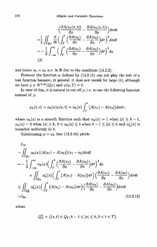
372 Elliptic and Parabolic Equations
/dA(ui(x,t)) _ dA(u2(x,t))\ V dx dx /
dxdt
-i£(jC(^-^H* <o
and hence u\ = u2 a.e. in R due to the condition (13.2.2). However the function tp denned by (13.2.11) can not play the role of a
test function because, in general, it does not vanish for large \x\, although we have tp S Wl<°°(QT) and tp{x,T) = 0.
In view of this, it is natural to cut-off <p, i.e. to use the following function instead of tp:
tpk(x,t)=ak(x)tp(x,t) = ak{x) / (A(ui) - A(u2))dxd,T,
where ak(x) is a smooth function such that ak(x) = 1 when \x\ < k — 1, ak{x) = 0 when \x\ > k, 0 < ak(x) < 1 when k — 1 < \x\ < k and a'k{x) is bounded uniformly in k.
Substituting <p = <pk into (13.2.10) yields
hk
= / / ak{x)(A{u\) - A(u2))(wi - u2)dxdt
s//8,oiw(/; w»,) - w x ^ - 5^)** =J2fc> (13.2.12)
where
Q r = {(a:,i) e Q T ; A ; - l < |x| <k,0<t<T}.
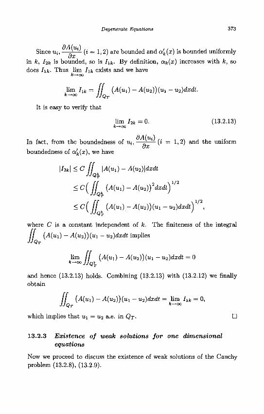
Degenerate Equations 373
dA(u) Since Ui, — (i = 1,2) are bounded and o/fe(x) is bounded uniformly
in k, lik is bounded, so is I\k- By definition, ak{x) increases with k, so does I\k- Thus lim I\k exists and we have
fc-»oo
lim Jlfe = / / (A(ui) - A(u2))(ui-U2)dxdt. IQT
It is easy to verify that
lim hk = 0. (13.2.13) k—»oo
In fact, from the boundedness of ut,—^- (i = 1,2) and the uniform ox
boundedness of a'k(x), we have
\hk\ <C [f \A{Ul) - A(u2)\dxdt JjQk
T
< C( ff (A(Ul) - A{u2)fdxdtjl 2
< C ( (J (A(«i) - A(u2))(ui - u2)dxdt} ,
where C is a constant independent of k. The finiteness of the integral
/ / (A(u\) — A(u2))(ui — u2)dxdt implies JJQT
lim / / (A(ui) - A{u2))(u\ -u2)dxdt = 0 =-"» J Jot
and hence (13.2.13) holds. Combining (13.2.13) with (13.2.12) we finally obtain
/ / (A(ui) - A(u2))(ui - u2)dxdt = lim hk = 0, JJQT fc^°°
which implies that u\ = u2 a.e. in QT- D
13.2.3 Existence of weak solutions for one dimensional equations
Now we proceed to discuss the existence of weak solutions of the Cauchy problem (13.2.8), (13.2.9).
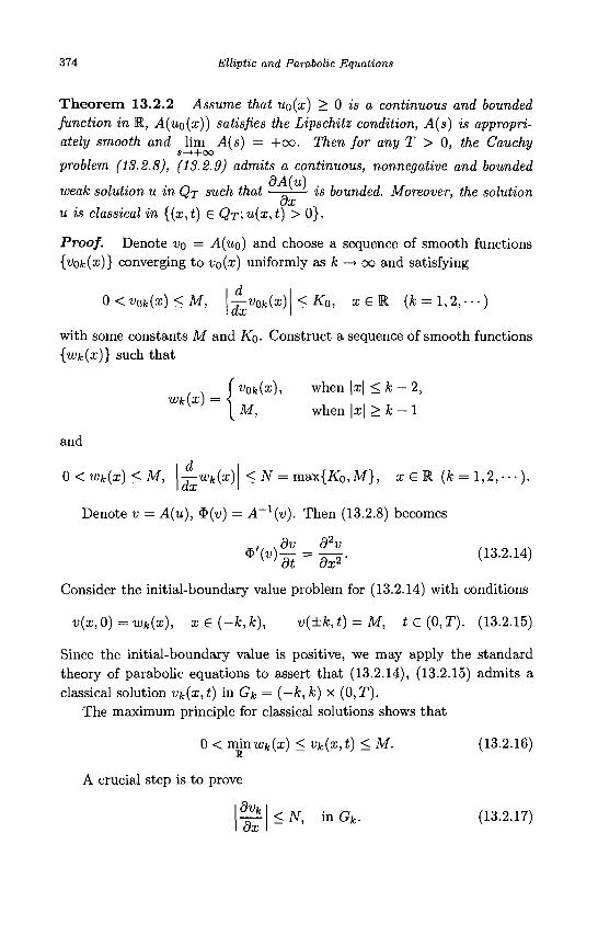
374 Elliptic and Parabolic Equations
Theorem 13.2.2 Assume that UQ(X) > 0 is a continuous and bounded function in R, A(uo(x)) satisfies the Lipschitz condition, A(s) is appropriately smooth and lim A(s) = +oo. Then for any T > 0, the Cauchy
s—»+oo
problem (13.2.8), (13.2.9) admits a continuous, nonnegative and bounded dA(u)
weak solution u in QT such that —^—^ is bounded. Moreover, the solution ox
u is classical in {(x,t) € Qr;u(x,t) > 0}.
Proof. Denote vo = A(uo) and choose a sequence of smooth functions {v0k(x)} converging to vo(x) uniformly as k —* oo and satisfying
0<vok(x)<M, -r-v0k{x) <K0, xeR (fc = l ,2 , ---)
with some constants M and KQ. Construct a sequence of smooth functions {u>k(x)} such that
Wk{x) = vok(x), when |x| < k — 2,
M, when |x| > k — 1
and
0<wk(x)<M, —wk(x)<N = max{K0,M}, x G R (k = 1,2, • • •) . ax
Denote v = A(u), $(i>) = A~l(v). Then (13.2.8) becomes
(13.2.14)
Consider the initial-boundary value problem for (13.2.14) with conditions
v(x,0) = wk(x), xe(-k,k), v(±k,t)=M, t € (0,T). (13.2.15)
Since the initial-boundary value is positive, we may apply the standard theory of parabolic equations to assert that (13.2.14), (13.2.15) admits a classical solution vk(x,t) in Gk = (—k,k) x (0,T).
The maximum principle for classical solutions shows that
0 < vnxnwk{x) < vk(x,t) < M. (13.2.16)
A crucial step is to prove
dvk dx
< N, in Gfc. (13.2.17)
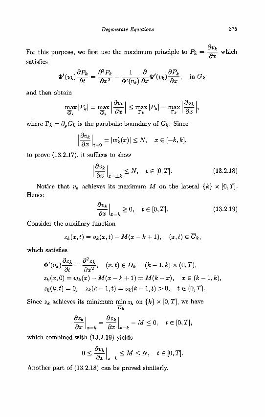
Degenerate Equations 375
For this purpose, we first use the maximum principle to Pk = -7-— which ox
satisfies
*'(«fc)
and then obtain
dPk d2Pk 1 d .,. ,dPk
-dT = -dxT--¥{^)-b-x^{vk)-dx-' mGk
max|Pfe| = max Gk Gk
dvk
dx < max|Pifc| = max
ovk
dx
where Tk = dpGk is the parabolic boundary of Gk- Since
dvk =\w'k(x)\<N, xe[-k,k], dx t=o
to prove (13.2.17), it suffices to show
dvk
dx x=±k <N, te[0,T}. (13.2.18)
Notice that vk achieves its maximum M on the lateral {k} x [0,T]. Hence
dvk dx x=k
>o, te[o,T]. (13.2.19)
Consider the auxiliary function
zk(x, t) = vk(x, t) - M(x - k + 1), (x, t) e Gk,
which satisfies
$ > f e ) l l = ' M € Dk = {k ~ 1,fc) X (°'T ) ' Zk(x,0) = wk(x) - M(x - k + l) = M(k - x), x e (k - l,k),
zk(k,t)=0, zk{k - l,t) = vk(k - l,t) > 0, i e ( 0 , T ) .
Since zk achieves its minimum minzk on {k} x [0, T], we have Dk
dzk
dx = dv^
x=k dx x=k M < O , ie[o,r],
which combined with (13.2.19) yields
dvk 0 < dx x=k
<M<N, t£[0,T}.
Another part of (13.2.18) can be proved similarly.
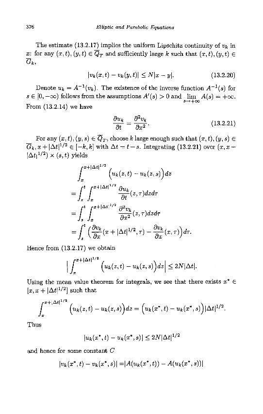
376 Elliptic and Parabolic Equations
The estimate (13.2.17) implies the uniform Lipschitz continuity of vk in x: for any (x,t), (y,t) £ QT and sufficiently large k such that (x,t), (y,t) €
\vk{x,t)-vk(y,t)\ <N\x-y\. (13.2.20)
Denote uk = A"1^). The existence of the inverse function A~1(s) for s e [0, +oo) follows from the assumptions A'(s) > 0 and lim A(s) = +oo.
3—*+00
Prom (13.2.14) we have
duk d2Vk
~i = -d- <1 3-2-2 1> For any (x, t), (y, s) € QT, choose k large enough such that (x, t), (y, s) €
Gk,x+ \At\l/2 £ [-k,k] with At = t-s. Integrating (13.2.21) over (a;,x + |At|1/2) x (s,t) yields
/ (uk(z,t) -uk(z,s)Jdz
=L L -^^dzdT
Hence from (13.2.17) we obtain
/ (uk(z, t) - uk(z, s))dz\ < 2N\At\. J x
Using the mean value theorem for integrals, we see that there exists x* £ [z.x + IA^I1/2] such that
fx+\At\^2 . / (uk(z,t)-Uk(z,s))dz= [uk(x*,t)-Uk(x*,s)J\At\1/2.
Thus
\uk(x*,t)-uk(x*,s)\<2N\At\1/2
and hence for some constant C
\vk(x*,t)-vk(x*,s)\=\A(uk(x*,t))-A(uk(x*,s))\
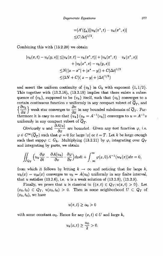
Degenerate Equations 377
=\A'(Zk)\\uk(x*,t)-uk(x*,s)\
<C\M\1'2.
Combining this with (13.2.20) we obtain
\vk(x,t) -vk(y,s)\ <\vk(x,t) -vk{x*,t)\ + \vk(x*,t) - vk(x*,s)\
+ \vk{x*,s) -vk(y,s)\
<N{\x - i*| + \x* - y\) + C\At\1/2
<(2AT + C ) ( | a ; - y | + |Ai|1/2)
and assert the uniform continuity of {vk} in Gk with exponent {1,1/2}. This together with (13.2.16), (13.2.18) implies that there exists a subsequence of {vk}, supposed to be {vk} itself, such that {vk} converges to a certain continuous function v uniformly in any compact subset of QT, and
\ -—— > weak star converges to -r— in any bounded subdomain of QT. Fur-K ax i ox
thermore it is easy to see that {uk} (uk = J 4 _ 1 ( ^ ) ) converges to u = A_1v uniformly in any compact subset of QT.
dA(u) Obviously u and —-— are bounded. Given any test function ip, i.e.
ox <p € C°°(QT) such that <p = 0 for large |x| or t = T. Let k be large enough such that suppy> C Gk- Multiplying (13.2.21) by <p, integrating over QT and integrating by parts, we obtain
L ("*£ " • D—+ £^0M-(«W)* - o, from which it follows by letting k —* oo and noticing that for large k, wk(x) = vok(x) converges to VQ = A(UQ) uniformly in any finite interval, that u satisfies (13.2.6), i.e. u is a weak solution of (13.2.8), (13.2.9).
Finally, we prove that u is classical in {(x,t) £ Qx;u(x,t) > 0}. Let (xo,to) G QT, u(xo,to) > 0. Then in some neighborhood U C QT of (xo,to), we have
u(x,t) > ao > 0
with some constant ao. Hence for any (x,t) G U and large k,
uk(x,t)>^->0.
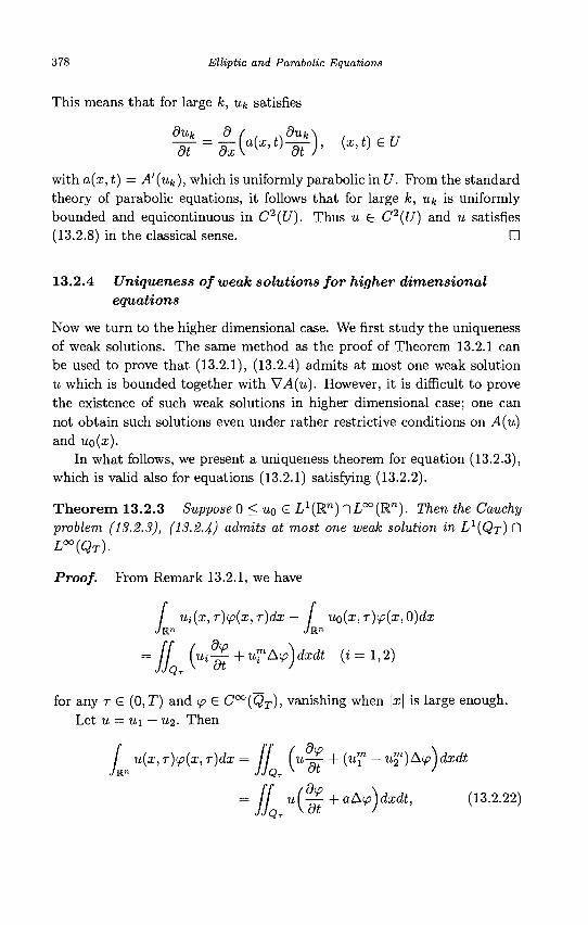
378 Elliptic and Parabolic Equations
This means that for large k, Uk satisfies
duk d ( ,sduk\ . . TT
with a(x, t) = A'(uk), which is uniformly parabolic in U. Prom the standard theory of parabolic equations, it follows that for large k, Uk is uniformly bounded and equicontinuous in C2(U). Thus u s C2(U) and u satisfies (13.2.8) in the classical sense. •
13.2.4 Uniqueness of weak solutions for higher dimensional equations
Now we turn to the higher dimensional case. We first study the uniqueness of weak solutions. The same method as the proof of Theorem 13.2.1 can be used to prove that (13.2.1), (13.2.4) admits at most one weak solution u which is bounded together with S7A(u). However, it is difficult to prove the existence of such weak solutions in higher dimensional case; one can not obtain such solutions even under rather restrictive conditions on A(u) and UQ(X).
In what follows, we present a uniqueness theorem for equation (13.2.3), which is valid also for equations (13.2.1) satisfying (13.2.2).
Theorem 13.2.3 Suppose 0<u0<= L 1(R n)nL°°(R n) . Then the Cauchy
problem (13.2.3), (13.2-4) admits at most one weak solution in L1{QT) n L°°{QT).
Proof. From Remark 13.2.1, we have
/ Ui(x,T)ip(x,T)dx — / uo(x,T)(p(x,0)dx
SJ dip Ui— +u™Atp\dxdt (i = 1,2)
for any r G (0,T) and <p 6 C°°(QT), vanishing when |a;| is large enough. Let u = iti — U2- Then
/ u(x,r)<p(x, r)dx = / / (u-£ + (uf - uf)Aip)dxdt
i(^+aAip\dxdt, (13.2.22) JJc
Ml
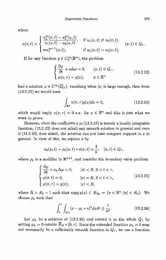
Degenerate Equations 379
where
' u?(x,t)-u2n(x,t)
a(x,t) , ifm(x,t)^u2(x,t),
ui(x,t) -u2(x,t)
mur[l~1(x,t), if ui(x,t) = U2(x,t),
If for any function g £ Co°(R"), the problem
dip
(x,t)€QT.
dt + aA<p = 0, (x,t)eQT,
<P(X,T) =g(x), xeM.n (13.2.23)
had a solution <p € C°°(QT), vanishing when \x\ is large enough, then from (13.2.22) we would have
/ u(x,r)g(x)dx = 0, (13.2.24)
which would imply u(x, r ) = 0 a.e. for x £ R" and this is just what we want to prove.
However, since the coefficient a in (13.2.23) is merely a locally integrable function, (13.2.23) does not admit any smooth solution in general and even if (13.2.23) does admit, the solution can not have compact support in x in general. In view of this, we replace a by
ak(x,t) = pk(x,t)*a(x,t) + T, (x,t) € QT, K
where pk is a mollifier in Rn + 1 , and consider the boundary value problem
( dip -^-+akA<p = 0, \x\ < R, 0 < t < T,
<p(x,t) = 0 ,
ip(x,r) =g(x),
\x\ = R, 0 < t < T,
\x\ < R,
(13.2.25)
where R > RQ + 1 such that supp<7(:r) C B^ = {x £ R"; \x\ < Ro}. We choose pk such that
fj Jo JE
a — pk* a)2dxdt < —^. BR *
(13.2.26)
Let ipk be a solution of (13.2.25) and extend it to the whole QT by setting <p>k = 0 outside BR X [0, r] . Since the extended function ipk = 0 may not necessarily be a sufficiently smooth function in QT, we use a function
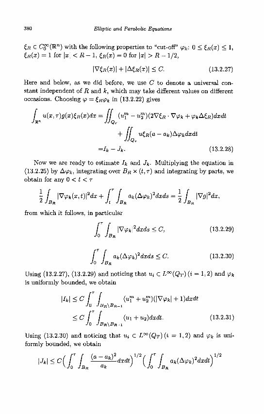
380 Elliptic and Parabolic Equations
£R G Cg°(R") with the following properties to "cut-off" <pk: 0 < £R(x) < 1, £R(x) = 1 for \x\<R- 1, £R(x) = 0 for \x\> R- 1/2,
| V 6 J ( Z ) | + | A 6 ? ( Z ) I < < ? . (13.2.27)
Here and below, as we did before, we use C to denote a universal constant independent of R and k, which may take different values on different occasions. Choosing <p — t,R<pk in (13.2.22) gives
/ u(x, T)g(x)£R(x)dx = if « - < ) ( 2 V 6 J • Vy>fe + <pkA£,R)dxdt JR" JJQ-r
+ / / u£R(a - ak)A<pkdxdt
=h + Jk. (13.2.28)
Now we are ready to estimate Ik and Jk. Multiplying the equation in (13.2.25) by A<pk, integrating over BR x (t,r) and integrating by parts, we obtain for any 0 < t < r
]-{ \V<pk(x,t)\2dx+ I I ak{A<pk)2dxds = )-f \Vg\2dx,
^ J BR Jt J BR ^ J BR
from which it follows, in particular
/ / \Vipk\2dxds<C, (13.2.29)
JO JBR
f f ak(Aipk)2dxds < C. (13.2.30)
Jo JBR
Using (13.2.27), (13.2.29) and noticing that ut e L°°{QT) (i = 1,2) and <pk
is uniformly bounded, we obtain
i4i <c r [ (u^+odv^i+i)dxdt Jo JBR\BR-!
<C f f (u1+u2)dxdt. (13.2.31) Jo JBR\BR-I
Using (13.2.30) and noticing that Uj £ L°°(QT){i = 1,2) and <pk is uniformly bounded, we obtain
\Jk\<c(fT f {a a
ak)2dxdt)l/\f j ak{Aykfdxdt) 1/2
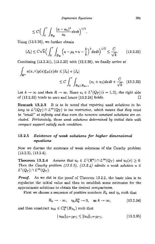
Degenerate Equations 381
<c([T f ^ ^ d x d t ) 1 / 2 . Wo JBR O-k '
Using (13.2.26), we further obtain
\Jk\<CVkN I (a - pk * a - ^ ) dxdt) < -=. (13.2.32)
Combining (13.2.31), (13.2.32) with (13.2.28), we finally arrive at
/ u(x,T)g(x)£R{x)dx < \Ik\ + \Jk\
<C I I (u1+u2)dxdt+-=. (13.2. Jo JBUXBR-! \ k
33)
Let k —> oo and then R —> oo. Since Ui S LX(QT) {i = 1,2), the right side of (13.2.33) tends to zero and hence (13.2.24) holds. •
Remark 13.2.3 It is to be noted that requiring weak solutions to belong to L}{QT) n L°°(QT) is too restrictive, which means that they must be "small" at infinity and thus even the nonzero constant solutions are excluded. Fortunately, those weak solutions determined by initial data with compact support satisfy such condition.
13.2.5 Existence of weak solutions for higher dimensional equations
Now we discuss the existence of weak solutions of the Cauchy problem (13.2.3), (13.2.4).
Theorem 13.2.4 Assume that u0 e L^M") n L°°(QT) and u0(x) > 0. Then the Cauchy problem (13.2.3), (13.2-4) admits a weak solution u € L\QT)f\L™{QT).
Proof. As we did in the proof of Theorem 13.2.2, the basic idea is to regularize the initial value and then to establish some estimates for the approximate solutions to obtain the desired compactness.
First we choose a sequence of positive numbers Rk and rjk such that
Rk -> +oo, r)kRl -> 0, as k -» oo, (13.2.34)
and then construct w0fc S Cg0 (£?#,.) such that
l|wofc||L~(M») < ||uo||z/»(R™)> (13.2.35)
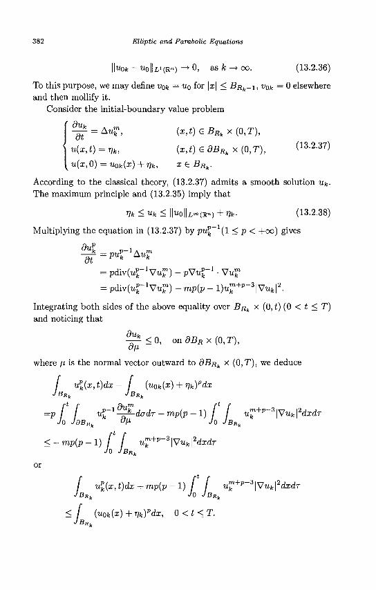
382 Elliptic and Parabolic Equations
\\uok - '"olU1(R") -» 0, as k —> oo. (13.2.36)
To this purpose, we may define Vok = UQ for \x\ < BRk-i, vok = 0 elsewhere and then mollify it.
Consider the initial-boundary value problem
^ = Auf, (x,t) e BRk x (0,T),
u(x, t)=t)k, (x, t) e dBRk x (0,T), (13.2.37)
u(x,0) =uok(x) + r)k, x£BRk.
According to the classical theory, (13.2.37) admits a smooth solution uk. The maximum principle and (13.2.35) imply that
Vk<uk< |KI |L°° (R«) + r)k. (13.2.38)
Multiplying the equation in (13.2.37) by pup~ (1 < p < +oo) gives
= pdiv(ul-1Vukn)-pVur1-Vuk
n
= p d i v K - V O - mp(p - l )^+ p - 3 |Vu f e | 2 .
Integrating both sides of the above equality over BRk x (0, t) (0 < t < T) and noticing that
^ < 0 , ondBRx(0,T),
where [i is the normal vector outward to dBRk x (0,T), we deduce
/ upk(x,t)dx- {uok(x)+-qk)
pdx JBRk JBRk
=P f I up-l^dadT-mp{p-l) f f u^+p~^uk\2dxdr
JO JdBRk "V h JBRk
<-mp(p-l) f [ u^+p~3\Vuk\2dxdT
Jo JBRk
or
/ up(x,t)dx + mp(p-l) f f u™+p-*\Vuk\2dxdT
JBRIC JO JBRk
<[ (uok(x)+rik)pdx, 0<t<T.
JB„,
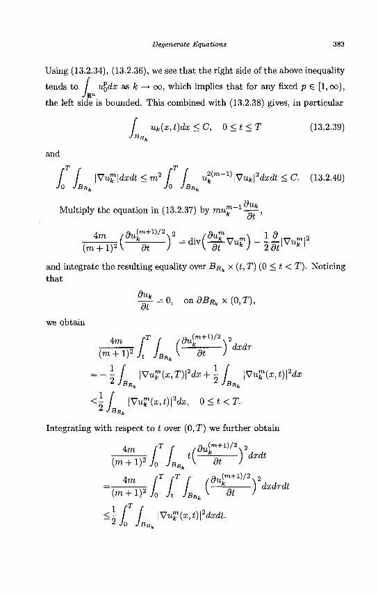
Degenerate Equations 383
Using (13.2.34), (13.2.36), we see that the right side of the above inequality
tends to / u*dx as k^ oo, which implies that for any fixed p € [l,oo),
the left side is bounded. This combined with (13.2.38) gives, in particular
/ uk(x, t)dx <C, 0<t<T (13.2.39)
and
f [ \VuZ\dxdt < m2 f f ul{m~l)\Vuk\2dxdt<C. (13.2.40)
JO JBRk JO JBRk
Multiply the equation in (13.2.37) by m « ™ " ' y ,
4m /d4m + 1 ) /V ,. (dvp_ m\ 19 ._ m | 2
and integrate the resulting equality over Bjik x (t, T) (0 < t < T). Noticing that
^ = 0 , ondBRkx(0,T),
we obtain
Am fT f / d 4 m + 1 ) / 2 N 2 j
wn?Jt LS-^-)dxdT
= - \ i \VuT(x,T)\2dx+\ f \VuT(x,t)fdx jB*k
JsRk
<\ ! \Vu%(x,t)\2dx, 0<t<T.
Integrating with respect to t over (0, T) we further obtain
Am fT f Jdu^+l),\2, M
<7i I f \Vuf(x,t)\2dxdt. M l |V 1 Jo JBR,
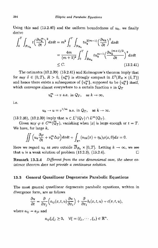
384 Elliptic and Parabolic Equations
Using this and (13.2.40) and the uniform boundedness of uk, we finally derive
< C. (13.2.41)
The estimates (13.2.39)-(13.2.41) and Kolmogrow's theorem imply that for any S G (0,T), R > 0, {u%} is strongly compact in L2(BR x (5,T)) and hence there exists a subsequence of {u™}, supposed to be {u™} itself, which converges almost everywhere to a certain function v in QT
u™ —> v a.e. in QT, as k —* oo,
i.e.
Uk —> u = u1 '"1 a.e. in QT, as fc —> OO.
(13.2.38), (13.2.39) imply that u G LX{QT) n L ° ° ( Q T ) -
Given any y> G Cco(QT), vanishing when \x\ is large enough or t = T. We have, for large k,
I (Uk~m + u™Av)dxdt + / (uok{x) + r)k)ip(x,Q)dx = 0.
Here we regard uk as zero outside BRk x [0,T]. Letting k —> oo, we see that u is a weak solution of problem (13.2.3), (13.2.4). •
Remark 13.2.4 Different from the one dimensional case, the above existence theorem does not provide a continuous solution.
13.3 General Quasilinear Degenerate Parabolic Equations
The most general quasilinear degenerate parabolic equations, written in divergence form, are as follows
where ay = a,ji and
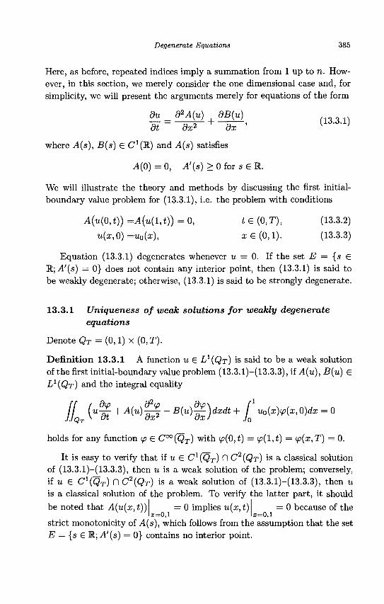
Degenerate Equations 385
Here, as before, repeated indices imply a summation from 1 up to n. However, in this section, we merely consider the one dimensional case and, for simplicity, we will present the arguments merely for equations of the form
du _ d2A(u) dB(u)
where A(s), B(s) G C^R) and A(s) satisfies
A(0) = 0, A'(s) > 0 for s G R.
We will illustrate the theory and methods by discussing the first initial-boundary value problem for (13.3.1), i.e. the problem with conditions
A(u(0,t)) =A(u(l,t)) = 0 , t G (0,T), (13.3.2)
u(x,0) =u0(x), Z G ( 0 , 1 ) . (13.3.3)
Equation (13.3.1) degenerates whenever u = 0. If the set £ = { s e R; A'(s) = 0} does not contain any interior point, then (13.3.1) is said to be weakly degenerate; otherwise, (13.3.1) is said to be strongly degenerate.
13.3.1 Uniqueness of weak solutions for weakly degenerate equations
Denote QT = (0,1) x (0,T).
Definition 13.3.1 A function u G LX{QT) is said to be a weak solution of the first initial-boundary value problem (13.3.1)-(13.3.3), if A(u), B(u) G L^iQr) and the integral equality
/ / ( U ^ + A ( U ) I? ~ B(u)%)dxdt + [ MxMx,0)dx = 0
holds for any function ip G C°°(QT) with tp(0,t) = <p(l,t) = <p(x,T) = 0.
It is easy to verify that if u G CX{QT) n C2(QT) is a classical solution of (13.3.1)-(13.3.3), then u is a weak solution of the problem; conversely, if u G C ^ Q r ) n C2(QT) is a weak solution of (13.3.1)-(13.3.3), then u is a classical solution of the problem. To verify the latter part, it should be noted that Aluix, t)) — 0 implies u(x, t) = 0 because of the
1=0,1 x=0,l
strict monotonicity of A(s), which follows from the assumption that the set E = {s G R; A'(s) = 0} contains no interior point.
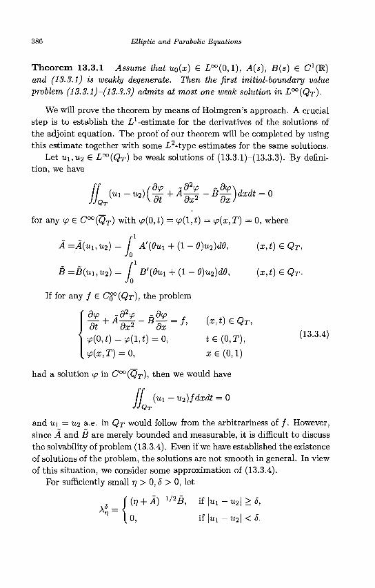
386 Elliptic and Parabolic Equations
Theorem 13.3.1 Assume that u0(x) G L°°(0,1), A(s), B(s) G C^R) and (13.3.1) is weakly degenerate. Then the first initial-boundary value problem (13.3.1)-(13.3.3) admits at most one weak solution in L°°(QT).
We will prove the theorem by means of Holmgren's approach. A crucial step is to establish the L1-estimate for the derivatives of the solutions of the adjoint equation. The proof of our theorem will be completed by using this estimate together with some L2-type estimates for the same solutions.
Let ui,u2 G L°°(QT) be weak solutions of (13.3.1)-(13.3.3). By definition, we have
JJo .<«-*>&+*S-*£)**=« (Ul-U2)(^+A-.
for any <p G C°°(QT) with tp(0,t) = <p(l,t) = <p(x,T) = 0, where
A =A(uuu2) = f A'(9Ul + (1 - e)u2)d6, (x,t) G QT, Jo
B =B(Ul, ua) = / B'{0ui + (1 - 6)u2)d6, (x, t)eQT-Jo
If for any / G CQ°(QT), the problem
' <p(o,t) = <p(i,t) = o, te(o,T), (13-3-4) ip{x,T) = Q, i G ( 0 , l )
had a solution tp in C°°(QT), then we would have
I (wi — u2)fdxdt = 0 QT
and ui — u2 a.e. in QT would follow from the arbitrariness of / . However, since A and B are merely bounded and measurable, it is difficult to discuss the solvability of problem (13.3.4). Even if we have established the existence of solutions of the problem, the solutions are not smooth in general. In view of this situation, we consider some approximation of (13.3.4).
For sufficiently small 77 > 0,5 > 0, let
g_ ((v + Ay^B, i f | u i - u 2 | > « ,
" l o , i f | u i - u 2 | < &
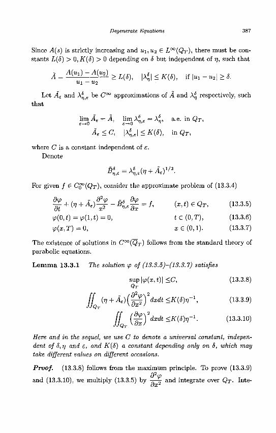
Degenerate Equations 387
Since A(s) is strictly increasing and u\,U2 € L°°(QT), there must be constants L(6) > 0, K(5) > 0 depending on 5 but independent of rj, such that
A=A(Ul)-A(u2)^ |A$| < * ( * ) , if | « x - « 2 l > J.
Let J4£ and A^£ be C°° approximations of A and A^ respectively, such that
lim As = A, lim A* = A*, a.e. in QT, e—0 e->0 n'e v
Ae<C, |A*,e| < A-(5), i n Q T ,
where C is a constant independent of e. Denote
S ^ A ^ + I,)1/2.
For given / G CQ°(QT), consider the approximate problem of (13.3.4)
l+(,+^-^&. V ( 0 J t ) = ¥ j ( l , t ) = 0 ,
^ ( i , T ) = 0 ,
= / , ( i , t ) € Q r ,
t e ( o , T ) ,
i e ( o , i ) .
(13.3.5)
(13.3.6)
(13.3.7)
The existence of solutions in C°°(QT) follows from the standard theory of parabolic equations.
13.3.1 The solution if of (13.3.5)-(13.3.7) satisfies
sup \ip{x,t)\ <C, QT
ff (r, + Ae)(^)2dxdt <K{8)t)-\
ffjg)'****™-1-
(13.3.8)
(13.3.9)
(13.3.10)
Here and in the sequel, we use C to denote a universal constant, independent of 5, rj and e, and K(5) a constant depending only on 5, which may take different values on different occasions.
Proof. (13.3.8) follows from the maximum principle. To prove (13.3.9)
and (13.3.10), we multiply (13.3.5) by -^-j and integrate over QT- Inte-
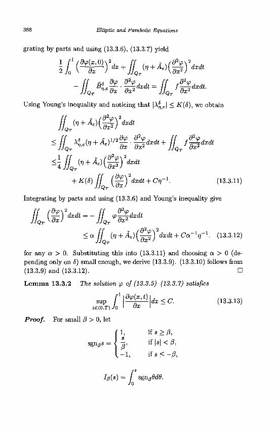
388 Elliptic and Parabolic Equations
grating by parts and using (13.3.6), (13.3.7) yield
Using Young's inequality and noticing that |A* | < K(S), we obtain
+ K(S) JJQT U J
dxdt + Cr]-1. (13.3.11)
Integrating by parts and using (13.3.6) and Young's inequality give
rdxdt
'<<*[[ {ri + Ae){-^\ dxdt + Ca-1^-1. (13.3.12)
for any a > 0. Substituting this into (13.3.11) and choosing a > 0 (depending only on 5) small enough, we derive (13.3.9). (13.3.10) follows from (13.3.9) and (13.3.12). •
L e m m a 13.3.2 The solution ip of (13.3.5)-(13.3.7) satisfies
f1 dip(x,t)
)Jo sup te(o,T).
dx dx<C. (13.3.13)
Proof. For small (3 > 0, let
sgn^s = < s
0'
if s > /?,
if \s\ < p,
if s < -0,
I0(s) = / sgn0ed6. Jo
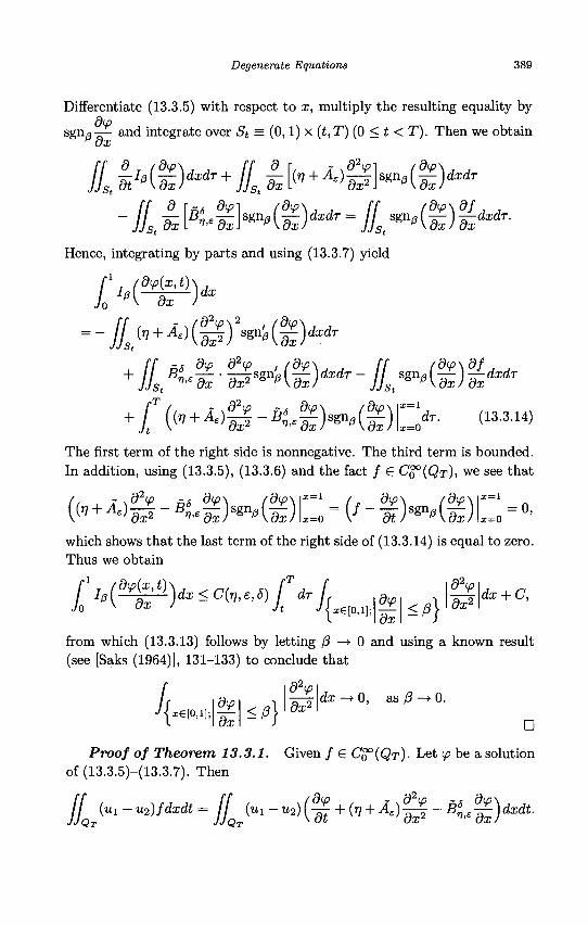
Degenerate Equations 389
Differentiate (13.3.5) with respect to x, multiply the resulting equality by
sgn^-^- and integrate over St = (0,1) x (t, T) (0 < t < T). Then we obtain
z^M sgn^ (tops \dx)
dxdr
Hence, integrating by parts and using (13.3.7) yield
-//<"+i-»(S)2^(l) dxdr
l^t•£-*(£)**- g-~>(%)%** / > + is) ay
dx2
B& 9<p\ fdipw*^1
' » ) .£ 9x W ^ ) [ > (13-3-14) The first term of the right side is nonnegative. The third term is bounded. In addition, using (13.3.5), (13.3.6) and the fact / 6 CQ°(QT), we see that
(e^>0-*!.SK(DC-('-|Wl)C-* which shows that the last term of the right side of (13.3.14) is equal to zero. Thus we obtain
[1lJ^-)dX<C(r},e,S)[TdrL Jo \ ox / j t Jixe[o, d<p
dx <0} I dx2 dx + C,
from which (13.3.13) follows by letting /? —» 0 and using a known result (see [Saks (1964)], 131-133) to conclude that
/ / xe[o,i]; dip
dx *»} \<frp I 9a; 2 dx —• 0, as /3 —> 0.
• Proof of Theorem 13.3.1. Given / € Cg°(QT)- Let ip be a solution
of (13.3.5)-(13.3.7). Then
/I" (ttl - u 2 ) / ^ = // (Ul - U2)(f + („ + * ) § - BH,.g)«fe*.
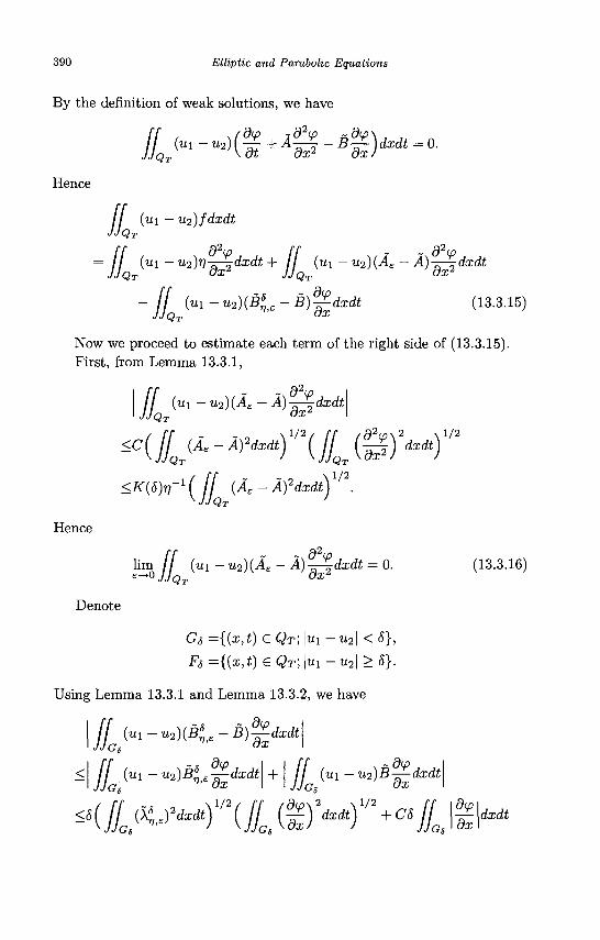
390 Elliptic and Parabolic Equations
By the definition of weak solutions, we have
Hence
1<--»>(!+4S-*S)**-°-
/ / (u i — u2)fdxdt JJQT
= / / (ui - u2)r]-Q^dxdt + / / (it! - u 2 ) ( i £ - A)-^dxdt
- If (ui - "2)(£*,e - B)^-dxdt (13.3.15)
Now we proceed to estimate each term of the right side of (13.3.15). First, from Lemma 13.3.1,
/ / (ui - W2)(A£ - A)-^dxdt
<c(£(i,-i)^)1/2(£(S)2H <A"(5)J7-1 ( If (Ae - Afdxdt)
1/2
IQT
,V2
Hence
lim / / rj2
(ui - u2)(A£ - A)—^dxdt = 0. (13.3.16)
Denote
Gs={{x,t)eQT;\ui-u2\ <6},
F5={(x,t)eQT;\u1-u2\ >6}.
Using Lemma 13.3.1 and Lemma 13.3.2, we have
JJ fa-mXB^-B^dxdt
< I II (ui - u2)B*iE-£dxdt + dip
/ / (ui — u2)B^-dxdt JJGS 9X
^JL^^niL^^^L dip
dx dxdt
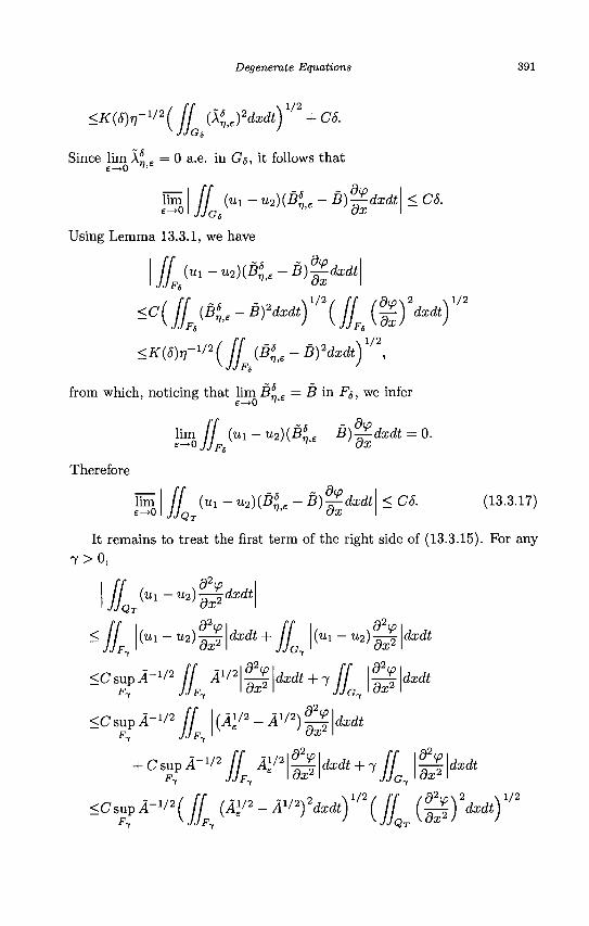
Degenerate Equations 391
<K(6)V-1/2 ( jj (XU2dxdt) V 2 + C5.
Since lim A*£ = 0 a.e. in Gs, it follows that
lim £—0
dtp <CS. jj (ui-u2)(B£e-.B)gdzdt
Using Lemma 13.3.1, we have
jj (Ul - u2)(BsVt£ - B)^dxdt
<K{5)rl/2(jjF {Ble - Bfdxdt)l'\
from which, noticing that lim Bt, = B in F$, we infer
1/2
SSj^< ui - u2)(5*>£ - B)^-dxdt = 0.
Therefore
lim £-*0
ff (m-UiHB^-B&dxdt JJQT
<CS. (13.3.17)
It remains to treat the first term of the right side of (13.3.15). For any
7 > 0 ,
} 2 ,
dxdt
jj (ui-u2)-^dxdt
-#J ( U 1 " U 2 ) & KCsupA-1'2 II A1
<C sup A-1'2 ff {A^-A1'2)
JJG-, u2)
1/2 9V 9a;2 dxdt + 7
d2<p
dx2
/ / ,
dxdt
dx2
dx2
dxdt
dxdt
C s u p A - 1 / 2 / / Al'2 d2v
dx2 dxdt + 7 JJG.
d2<p
dx2 dxdt
«v i / 2(/i w2-A"^y'VL (S)2H 1/2
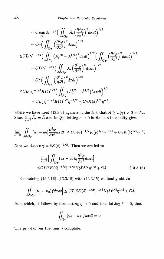
392 Elliptic and Parabolic Equations
<CL(7)-1/2#(<5)1/2 ( jj (A\'2 - A^fdxdt) V 2
+ CL[n)-V2K{6)V2rrV2 + C-yKtf)1'2*-1,
where we have used (13.3.9) again and the fact that A > L(j) > 0 in F7 . Since lim Ae = A a.e. in QT, letting e —> 0 in the last inequality gives
£—>0
d2
(ui -u2)-IQT
(
Now we choose 7 = 5K{5)~1/2. Then we are led to
32
lim E-»0
II («i - u2)^dxdt < CL^)-1'2^)1'2^2 + CjKiS)1^-1.
jj (ui - u2)r]-—^dxdt
<Ci(5JftT(5)-1/2)-1/2ir(^)1/2771/2 + CS. (13.3.18)
lim £- •0
Combining (13.3.16)-(13.3.18) with (13.3.15) we finally obtain
II («i - u2)fdxdt < CLiSKiSy^y^KiS)1/2^2 + CS, JJQT
from which, it follows by first letting 77 —> 0 and then letting 5 —> 0, that
/ / ("l — u2)fdxdt = 0. >Q
The proof of our theorem is complete.
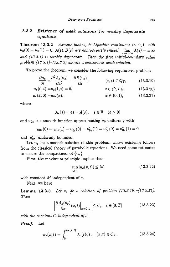
Degenerate Equations 393
13.3.2 Existence of weak solutions for weakly degenerate equations
Theorem 13.3.2 Assume that UQ is Lipschitz continuous in [0,1] with uo(0) = wo(l) = 0, A(s),B(s) are appropriately smooth, lim A(s) = ±00
s—>±oo
and (13.3.1) is weakly degenerate. Then the first initial-boundary value problem (13.3.1)-(13.3.3) admits a continuous weak solution.
To prove the theorem, we consider the following regularized problem
duE d2A£(ue) dB{u£) (rrt^n M „ 1 0 l
-df=—dxl- + -&r> (x,t)£QT, (13.3.19)
ue(0,t) =u£(l,t) = 0, t e ( 0 , T ) , (13.3.20)
ue(a;,0) =ti0e(a;), x G (0,1), (13.3.21)
where
Ae{s) =es + A{s), s£R (e > 0)
and uoe is a smooth function approximating UQ uniformly with
"0,(0) = u0E(l) = 4 , ( 0 ) - «oe(l) = <{0) = 1^(1) = 0
and |u0e| uniformly bounded. Let ue be a smooth solution of this problem, whose existence follows
from the classical theory of parabolic equations. We need some estimates to ensure the compactness of {ue}.
First, the maximum principle implies that
sup\uE{x,t)\ < M (13.3.22) QT
with constant M independent of e. Next, we have
Lemma 13.3.3 Let u€ be a solution of problem (13.3.19)-(13.3.21).
Then
dx V ' ; 1=0,1
with the constant C independent of e.
Proof. Let
we(x,t)= r X ' X€(s)ds, (x,t)£QT, (13.3.24) Jo
<C, te[0,T} (13.3.23)
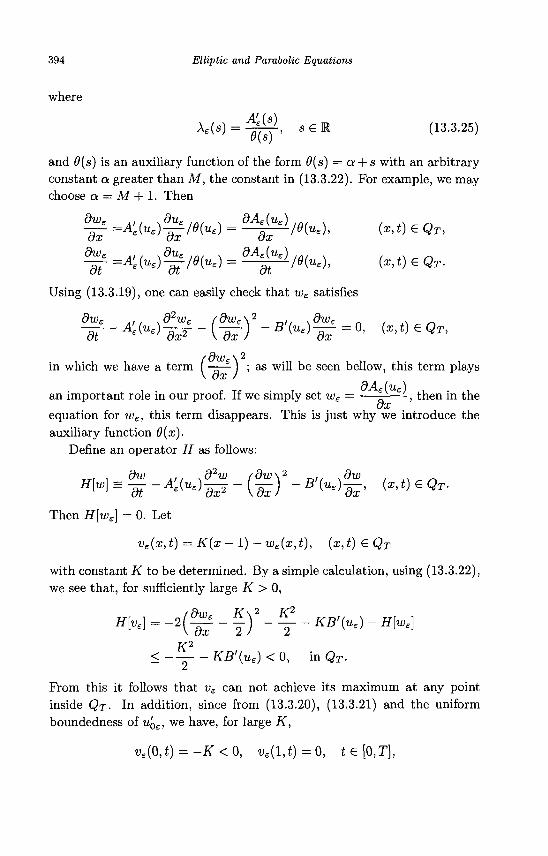
394 Elliptic and Parabolic Equations
where
Ae(s) = f SGR (13'3-25) and 6(s) is an auxiliary function of the form 6(s) = a + s with an arbitrary constant a greater than M, the constant in (13.3.22). For example, we may choose a = M + 1. Then
dwE . . . sdu€ ,„. . dAJur) ,„. . ^ - ^ =^(«e)-^/fl(«e) = e
dy>/6(u€), (x,t) e QT, 9W£ w / % ^ U £ / „ , -, 9 j 4 £ ( u e ) . . . . , . „ ~Qf =A'e(Ue)-gf/6(Ue) = —^-/0(ue), (X,t) € QT-
Using (13.3.19), one can easily check that we satisfies
in which we have a term I - j—^ j ; as will be seen bellow, this term plays
dA (u ) an important role in our proof. If we simply set w£ = —|——, then in the
ox equation for we, this term disappears. This is just why we introduce the auxiliary function 6{x).
Define an operator H as follows:
r r r . dw . . . .d2w /dw\2 , .dw . _, H [ U , ] S _ - ^ ( U B ) _ - ( _ ) -B'(US)-, (X,t)GQr.
Then H[w£] = 0. Let
ve(x, t) = K(x — 1) — we(x,t), (x,t)eQT
with constant K to be determined. By a simple calculation, using (13.3.22), we see that, for sufficiently large K > 0,
K2
<-—-KB'(ue)<0, inQT.
From this it follows that ve can not achieve its maximum at any point inside QT. In addition, since from (13.3.20), (13.3.21) and the uniform boundedness of u'0e, we have, for large K,
ve(0,t) =-K < 0, ve(l,t) = 0, te[0,T],
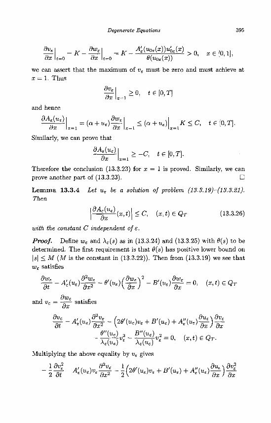
Degenerate Equations 395
dv£
dx t=o ox = y_^yx))y)> x
t=o 6(u0£{x))
we can assert that the maximum of u£ must be zero and must achieve at i = l. Thus
and hence
dA£(u£)
dv£
dx x-1 >o, te[o,T]
dx = {a + u£)-^-
x=l OX <(a + u£) K<C, te[0,T].
x=l x=l
Similarly, we can prove that
dA£(ue)
dx x=l >-C, t€[0,T\.
Therefore the conclusion (13.3.23) for x = 1 is proved. Similarly, we can prove another part of (13.3.23). •
Lemma 13.3.4 Let u£ be a solution of problem (13.3.19)-(13.3.21). Then
dA£{u£)
dx (x,t) <C, {x,t)GQT (13.3.26)
with the constant C independent of e.
Proof. Define w£ and X£(s) as in (13.3.24) and (13.3.25) with 6(s) to be determined. The first requirement is that 6(s) has positive lower bound on \s\ < M (M is the constant in (13.3.22)). Then from (13.3.19) we see that wF satisfies
dwe d2w£ „ , , s/dw£\2 „ , , sdw£
u£)
satisfies
- A ' M ^ -e'^(^ty -B>^=°. («.«)e QT dt "e^ej dx2
and vE = dx
dve
dt *wf£-(*<**+ * « + *(-.)£)£ 6"(u£) 3 B"(u£) o n . . n
Multiplying the above equality by ve gives
1 dv2 . . . . d2v£ 1/„. , , . „ , , . . „ . sdue\ 2 dt dx2
du£ \ dv2
dx
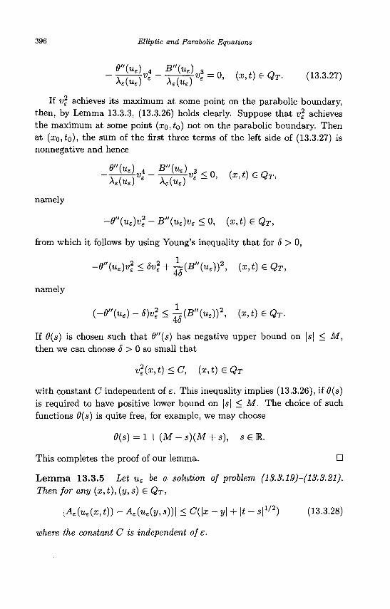
396 Elliptic and Parabolic Equations
- S t y " = - S r » . 3 = ° . <*.«>s«- <13-3-27> If u2 achieves its maximum at some point on the parabolic boundary,
then, by Lemma 13.3.3, (13.3.26) holds clearly. Suppose that v2e achieves
the maximum at some point (xo,£o) n o t o n t n e parabolic boundary. Then at (zo,£o), the sum of the first three terms of the left side of (13.3.27) is nonnegative and hence
6"(uE) 4 B"(uE) 3 n . . ^ \E\uE) A£(ue)
namely
-6"{uE)v2£ - B"(uE)vE < 0, (x, t) e QT,
from which it follows by using Young's inequality that for 5 > 0,
-e"(ue)v2£ < 6vl + 1 ( B > £ ) ) 2 , (X,t) G Qr ,
namely
( - 0 > e ) - <5K2 < ^ (B"K)) 2 , (i,t) e Q r .
If 6(s) is chosen such that 8"(s) has negative upper bound on \s\ < M, then we can choose S > 0 so small that
u2(z,t)<C, (x,t)eQT
with constant C independent of e. This inequality implies (13.3.26), if #(s) is required to have positive lower bound on \s\ < M. The choice of such functions 6(s) is quite free, for example, we may choose
0(s) = l + (M-s)(M + s), s£R.
This completes the proof of our lemma. •
Lemma 13.3.5 Let u£ be a solution of problem (13.3.19)-(13.3.21). Then for any (x, t), (y, s) e QT,
\AE(uE(x, t)) - AE(ue(y, s))\ < C(\x -y\ + \t- s|1/2) (13.3.28)
where the constant C is independent of e.
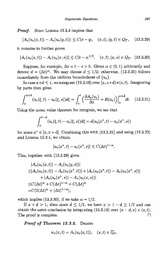
Degenerate Equations 397
Proof. Since Lemma 13.3.4 implies that
\A£(u£{x,t))-A£(u£(y,t))\<C\x-y\, (x,t),(y,t) e QT, (13.3.29)
it remains to further prove
| A £ ( n £ ( x , 0 ) - ^ ( w £ ( x , s ) ) | < C | t - s | 1 / 2 , {x,t),(x,s)£QT. (13.3.30)
Suppose, for example, At = t — s > 0. Given a £ (0,1) arbitrarily and denote d = (At)a. We may choose d < 1/2; otherwise, (13.3.30) follows immediately from the uniform boundedness of {u£}.
In case x+d < 1, we integrate (13.3.19) over (x, x+d) x (s, t). Integrating by parts then gives
rx+d /"' /3A (11 \ \ \*+d J (ue(U)-ue(Z,s))d£ = J (?-J±-±L + B(ue))\x dt. (13.3.31)
Using the mean value theorem for integrals, we see that
/ J X
(u£(t,t)-u£(£,s))dZ = d(u£(x*,t)-u£{x*,s))
for some x* G [x,x + d]. Combining this with (13.3.31) and using (13.3.22) and Lemma 13.3.4, we obtain
\ue(x*,t) - u£{x*, s)\ < C(At)1-01.
This, together with (13.3.29) gives
\A£{u£{x,t))-A£(u£(y,s))\
<\A£(u£(x,t))-A£(u£(x*,t))\ + \A£(u£(x*,t))-A£(u£(x*,s))\
+ \A£(u£(x*,s))-A£(u£{x,s))\
<C(At)a + C ( A i ) 1 _ a + C{At)a
=C(2{At)a + (At)1-0),
which implies (13.3.30), if we take a = 1/2. If x + d > 1, then since d < 1/2, we have x > 1 — d > 1/2 and can
obtain the same conclusion by integrating (13.3.19) over (x — d, x) x (s,t). The proof is complete. •
Proof of Theorem 13.3.2. Denote
w£(x, t) = A£(u£(x, t)), (x, t) e QT.
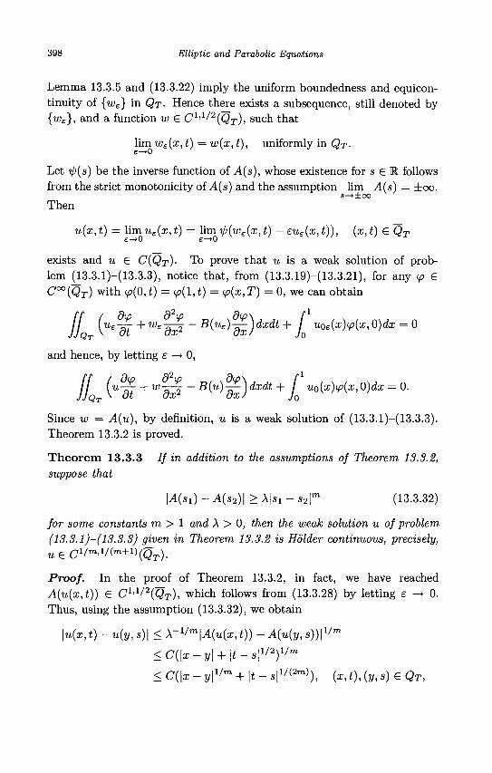
398 Elliptic and Parabolic Equations
Lemma 13.3.5 and (13.3.22) imply the uniform boundedness and equicon-tinuity of {we} in QT- Hence there exists a subsequence, still denoted by {w£}, and a function w G Cl'1/2(QT), such that
lim we(x, t) = w(x, t), uniformly in QT-e—>0
Let tp(s) be the inverse function of A(s), whose existence for s G R follows from the strict monotonicity of A(s) and the assumption lim A(s) = ±oo.
s—»±oo
Then
u(x, t) = lim ue(x, t) = lim ip(w€(x, t) — eu£(x, t)), (x, t) G QT
exists and u G C{QT)- To prove that u is a weak solution of problem (13.3.1)-(13.3.3), notice that, from (13.3.19)-(13.3.21), for any <p e C°°(QT) with <p(Q,t) = <p(l,t) = <p(x,T) = 0, we can obtain
n n r\ {lis S3 P1
/ / (u£—+WE-Q-^-B(ue)—)dxdt+ uOs(x)ip(x,0)dx = 0
and hence, by letting e —> 0,
I [u-^ + w — ^ - B{u)-^Pjdxdt + J u0(x)tp(x,0)dx = 0.
Since w = A(u), by definition, u is a weak solution of (13.3.1)—(13.3.3). Theorem 13.3.2 is proved.
Theorem 13.3.3 If in addition to the assumptions of Theorem 13.3.2, suppose that
\A(si) - A(s2)\ > \\si - s2\m (13.3.32)
for some constants m > 1 and A > 0, then the weak solution u of problem (13.3.1)-(13.3.3) given in Theorem 13.3.2 is Holder continuous, precisely, u e C l / m , l / ( m + l ) ( Q T ) _
Proof. In the proof of Theorem 13.3.2, in fact, we have reached A{u{x,t)) e C 1 , 1 / 2 (QT ) , which follows from (13.3.28) by letting e -> 0. Thus, using the assumption (13.3.32), we obtain
\u{x,t)-u{y,s)\<\-llm\A{u{x,t))-A{u{y,s))\llm
<C(\x-y\ + \t-s\1'2)llm
< C{\x - y\l/m + \t- s\^2^), (x, t), (y, s) G QT,
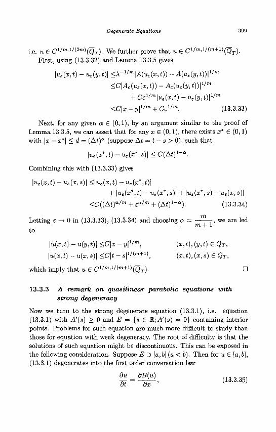
Degenerate Equations 399
i.e. u G Cl/m'l/{2m){QT). We further prove that u G C1/m-1/(m+1)(QT). First, using (13.3.32) and Lemma 13.3.5 gives
\u£(x,t)~u£(y,t)\<X^m\A(ue(x,t))-A(u£(y,t))\1/m
<C\A£(u£(x,t)) - A£(ue(y,t))\1/m
+ Ce1/m\u£(x,t)-u£(y,t)\1/m
<C\x-y\1/m + Ce1/m. (13.3.33)
Next, for any given a G (0,1), by an argument similar to the proof of Lemma 13.3.5, we can assert that for any x G (0,1), there exists x* G (0,1) with \x — x*\ < d = (At)a (suppose At = t — s > 0), such that
\u£(x*,t)-u£(x*,s)\ < C{Atf~a.
Combining this with (13.3.33) gives
\us(x,t) - ue(x,s)\ <\u£(x,t) — ue(x*,t) |
+ \u£(x*,t) -u£(x*,s)\ + \u£(x*,s) -ue(x,s)\
<C((At)a/m + ea/m + (At)l-a). (13.3.34)
TYl
Letting e —» 0 in (13.3.33), (13.3.34) and choosing a = - , we are led to
\u(x, t) - u(y, t)\ <C\x - y\Vm, (x, t), (y, t) G QT,
\u(x,t)-u{x,s)\ <C\t-s\1/{m+1\ (x,t),(x,s)£QT,
which imply that u G C 1 / m ' 1 / ( m + 1 ) (Qr ) - n
13.3.3 A remark on quasilinear parabolic equations with strong degeneracy
Now we turn to the strong degenerate equation (13.3.1), i.e. equation (13.3.1) with A'(s) > 0 and E = {s G R;A'(s) = 0} containing interior points. Problems for such equation are much more difficult to study than those for equation with weak degeneracy. The root of difficulty is that the solutions of such equation might be discontinuous. This can be exposed in the following consideration. Suppose E D [a,b] (a <b). Then for u G [a, b], (13.3.1) degenerates into the first order conversation law
du _ dB{u)
dt dx (13.3.35)
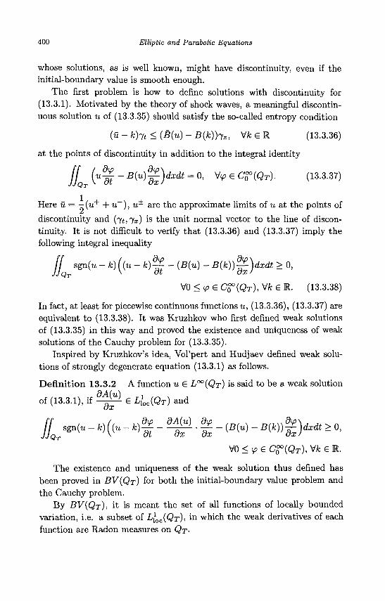
400 Elliptic and Parabolic Equations
whose solutions, as is well known, might have discontinuity, even if the initial-boundary value is smooth enough.
The first problem is how to define solutions with discontinuity for (13.3.1). Motivated by the theory of shock waves, a meaningful discontinuous solution u of (13.3.35) should satisfy the so-called entropy condition
(u-k)jt<(B(u)-B(k))ix, VfceR (13.3.36)
at the points of discontinuity in addition to the integral identity
fj (u^-B(u)^dxdt = 0, V eCo°°(QT). (13.3.37)
Here u = —{u+ +u~), u^ are the approximate limits of u at the points of discontinuity and (74,7x) is the unit normal vector to the line of discontinuity. It is not difficult to verify that (13.3.36) and (13.3.37) imply the following integral inequality
jj sgn(« - *)((« ~k)^- (B(u) - B{k))^)dxdt > 0,
V0 < <p G C%°{QT), Vfc e R. (13.3.38)
In fact, at least for piecewise continuous functions u, (13.3.36), (13.3.37) are equivalent to (13.3.38). It was Kruzhkov who first denned weak solutions of (13.3.35) in this way and proved the existence and uniqueness of weak solutions of the Cauchy problem for (13.3.35).
Inspired by Kruzhkov's idea, Vol'pert and Hudjaev denned weak solutions of strongly degenerate equation (13.3.1) as follows.
Definition 13.3.2 A function u € L°°(QT) is said to be a weak solution
of (13.3.1), if ^ € Llc(QT) and
£ sgn(„ - *,((. - » , | - <^>. fe - <*(., - *(* , ) ! )** > 0, VO < ^ e C H Q T ) , Vfc e R.
The existence and uniqueness of the weak solution thus defined has been proved in BV(QT) for both the initial-boundary value problem and the Cauchy problem.
By BV(QT), it is meant the set of all functions of locally bounded variation, i.e. a subset of L\OC{QT), in which the weak derivatives of each function are Radon measures on QT-
Degenerate Equations 401
The existence can be proved by means of parabolic regularization; the basic idea is the same as the proof of Theorem 13.3.2 but it is different in techniques. The proof of uniqueness is rather difficult, which is based on a deep study of functions in BV(QT) and a complicated derivation (see [Wu, Zhao, Yin and Li (2001)]).

Bibliography
Adams R. A., Sobolev Spaces, Academic Press, New York-London, 1975. Chen Yazhe, Parabolic Equations of Second Order, Beijing University Press,
China, 2003. Chen Yazhe and Wu Lancheng, Elliptic Equations and Systems of Second Order,
Science Press, China, 1997. Cui Zhiyong, Jin Dejun and Lu Xiguan, Introduction to Linear Partial Differential
Equations, Jilin University Press, 1991. Evans L. C , Weak Convergence Methods for Nonlinear Partial Differential Equa
tions, CBMS 74, American Mathematical Society, Providence, RI, 1990. Friedman A., Partial Differential Equations of Parabolic Type, Pentice-Hall, Inc.,
1964. Gilbarg D. and Trudinger N. S., Elliptic Partial Differential Equations of Second
Order, Springer-Verlag, Heidelberg-New York, 1977. Gu Liankun, Parabolic Equations of Second Order, Xiamen University Press,
1995. Jiang Zejian and Sun Shanli, Functional Analysis, Higher Education Press, 1994. Ladyzenskaja O. A., Solonnikov V. A. and Ural'ceva N. N., Linear and Quasi-
linear Equations of Parabolic Type, TransL Math. Mono., 23, American Mathematical Society, Providence, RI, 1968.
Ladyzenskaja O. A. and Ural'ceva N. N., Linear and Quasilinear Elliptic Equations, English TransL, Academic Press, New York, 1968.
Lieberman G. M., Second Order Parabolic Differential Equations, World Scientific Publishing Co., Inc., River Edge, NJ, 1996.
Maz'ja V. G., Sobolev Spaces, English TransL, Springer-Verlag, Berlin-Heidelberg, 1985.
Oleinik O. A. and Radkevic E. V., Second Order Differential Equations with Nonnegative Characteristic Form, American Mathematical Society, Rhode Island and Plenum Press, New York, 1973.
Pao C. V., Nonlinear Parabolic and Elliptic Equations, Plenum Press, New York, 1992.
Saks S., Theory of the Integral, English TransL, Dover Publications, Inc., New York, 1964.
403
404 Elliptic and Parabolic Equations
Wu Zhuoqun, Zhao Junning, Yin Jingxue and Li Huilai, Nonlinear Diffusion Equations, World Scientific Publishing Co., Singapore, 2001.
Zhong Chengkui, Fan Xianling and Chen Wenyuan, Introduction to Nonlinear Functional Analysis, Lanzhou University Press, 1998.
Index
ck(n), 2 Cff(n), 2 Ck'a(Q), 7 ck<a(n,), 7 Hk(Q), 15 I? theory, 39, 60, 71, 94, 241, 256 L°° norm estimate, 233, 264 W estimate, 255, 260, 264, 266, 271 LP norm estimate, 264, 273 V(QT), 24 V2{QT), 24
W2k'k{QT), 24 Wk*(p), 15 ^ • p ( n ) , 15 BMO(Qo), 259
W2pk'k(QT), 24
W?'"{QT), 24
t-anisotropic Campanato space, 197 t-anisotropic Poincare's inequality,
28, 204 t-anisotropic Sobolev space, 24 t-anisotropic embedding theorem, 26
relatively strongly compact, 16
a modified Lax-Milgram's theorem, 73,94
Aleksandrov's maximum principle, 264, 273
Arzela-Ascoli's theorem, 241
barrier function, 291, 293 barrier function technique, 242, 282 Bernstein approach, 282, 296, 297 bilinear form, 64 boundary gradient estimate, 282, 287,
289 boundary Holder's estimate, 287, 289 boundary Holder's estimate for
gradients, 308
Caccioppoli's inequality, 168, 200, 205, 208
Campanato space, 160, 198, 256 Cauchy problem, 369 Cauchy's inequality, 1 Cauchy's inequality with e, 2 classical Harnack's inequality, 133 coercive, 64 compact continuous field, 316 compact continuous mapping, 315 compact embedding theorem, 20 comparison principle, 233, 235, 238 completely continuous field, 316 completely continuous mapping, 315 conjugate operator, 48 continuity module, 261 contraction mapping principle, 246 coupled elliptic system, 354 coupled parabolic system, 336 critical point, 314 critical value, 314 cut-off function, 5
405
406 Elliptic and Parabolic Equations
De Giorgi iteration, 105, 110, 115, 282 degenerate equation, 355 diagonal process, 244 difference operator, 47 Dirichlet problem, 39 discontinuous solution, 400 domain additivity, 315, 317 domain of (A)-type, 160
Ehrling-Nirenberg-Gagliardo's interpolation inequality, 17, 260
elliptic regularization, 365 embedding theorem, 19, 204 energy method, 71, 94 entropy condition, 400 estimate near the boundary, 122 existence and uniqueness of the
classical solution, 240, 248-251 existence and uniqueness of the
strong solution, 264, 272 existence and uniqueness of the weak
solution, 46, 62, 75 existence of classical solutions, 233 exterior ball property, 242
Fichera function, 356 filtration equation, 368 fixed point method, 277 Fredholm's alternative theorem, 67
Galerkin's method, 85, 101 general elliptic equations, 60, 187 general linear elliptic equations, 248,
260 general linear parabolic equations,
251, 271 general parabolic equations, 94, 231 general quasilinear degenerate
parabolic equations, 384 global estimate, 193 global gradient estimate, 282, 296 global Holder's estimate for gradients,
310 global regularity, 56, 92
Holder space, 7
Holder's estimate, 143, 155, 282, 301 Holder's estimate for gradients, 282,
307 Holder's inequality, 2 Harnack's inequality, 131, 141, 145,
156, 282, 284 heat equation, 71, 111, 123, 199, 250,
266 heat equation with strong nonlinear
source, 317 Hilbert-Schmidt's theorem, 85 homogeneous heat equation, 111, 123,
145
in the sense of distributions, 41 integral characteristic of Holder
continuous functions, 161, 198 interior estimate, 178, 200 interior Holder's estimate, 155, 284 interior Holder's estimate for
gradients, 307 interior regularity, 50 interpolation inequality, 17, 200 invariance of compact homotopy, 317 invariance of homotopy, 315 inverse Holder's inequality, 125 inverse Poincare's inequality, 124 iteration lemma, 177, 205, 207, 213,
301
Kronecker's existence theorem, 315, 317
Laplace's equation, 105, 118, 131 Lax-Milgram's theorem, 64 Leray-Schauder degree, 315 Leray-Schauder's fixed point theorem,
277 linear elliptic equation, 240, 255, 264 linear parabolic equation, 249, 272 Lipschitz space, 8 local boundedness estimate, 116, 118,
120, 121, 123, 126 local flatting, 6 lower sequence, 325
Bibliography 407
maximum estimate, 282 maximum principle, 233, 237, 241,
282 mean value formula, 131 method of continuity, 246 method of solidifying coefficients,
188, 263 Minkowski's inequality, 2 mixed quasimonotone, 337 mollifier, 4 monotone method, 323 monotone sequence, 339 more general quasilinear elliptic
equations, 310 more general quasilinear equations,
310 more general quasilinear parabolic
equations, 311 Morrey's theorem, 282, 302 Moser iteration, 105, 121, 123, 137,
282, 285
near bottom estimate, 211 near boundary estimate, 181, 191 near lateral boundary estimate, 219 nonhomogeneous heat equation, 112,
126 normality, 314, 316
one-sided Lipschitz condition, 324 ordered supersolution and
subsolution, 324, 338
partition of unity, 6 Poincare's inequality, 21, 28 Poisson's equation, 39, 47, 107, 120,
122, 178, 181, 240, 255, 287 property of segment, 16 property of uniform inner cone, 17
quasilinear degenerate parabolic equation, 368
quasilinear elliptic equation, 277 quasilinear parabolic equation, 280 quasimonotone, 337 quasimonotone nondecreasing, 337
quasimonotone nonincreasing, 337
regular point, 313 regular value, 314 regularity near the boundary, 53 regularity of weak solutions, 47, 50,
89 relatively weakly compact, 16 rescaling, 23, 204 Riesz's representation theorem, 41, 61 Rothe's method, 79, 96
Schauder's estimate, 159, 187, 197, 199, 231, 233, 264
Schwarz's inequality, 2 sector, 324, 339 semi-difference method, 79 shock wave, 400 sign rule, 297 smoothing operator, 3, 58 Sobolev conjugate exponent, 20 Stampacchia's interpolation theorem,
259 strong solution, 255, 263, 266, 272 strongly compact, 16 strongly degenerate, 385 subelliptic operator, 368 subellipticity, 368 subsolution, 324, 338 supersolution, 324, 338 support, 3
test function, 51, 54, 72, 73, 370-372, 377
the first boundary value problem, 356 the first initial-boundary value
problem, 71 topological degree, 313 topological degree method, 313 trace of functions in H1 (fi), 29
uniform exterior ball property, 242 uniform parabolicity, 94, 231 uniformly elliptic, 60 upper sequence, 325
408 Elliptic and Parabolic Equations
weak derivative, 14 weak supersolution, 116, 123 weak Harnack's inequality, 154, 284 weakly compact, 16 weak maximum principle, 105, 107, weakly degenerate, 385
111, 112 weak solution, 40, 60, 361, 362, 369, Young's inequality, 1
370, 385 Young's inequality with e, 2 weak subsolution, 116, 123
,^i.
.•
Elliptic & Parabolic Equations This' book provides an introduction to elliptic and parabolic
equations. While there are numerous monographs focusing
separately on each kind of equations, there are very few
books treating these two kinds of equations in combination.
This book presents the related basic theories and methods
to enable readers to appreciate the commonalities between
these two kinds of equations as well as contrast the similarities
and differences between them.
YEARS OF P U B L I S H I N G
ISBN 981-270-025-0
9 "789812' 700254
www.worldscientific.co


![Continuity of Solutions of Parabolic and Elliptic ... · The theory of non-linear elliptic equations in two independent variables is fairly well developed. (See [I] for a survey and](https://img.pdfslide.net/doc/110x75/5fdb11646c72d709f721b6cb/continuity-of-solutions-of-parabolic-and-elliptic-the-theory-of-non-linear-elliptic.jpg)