Endogenous Product Qualities, Financial Structure, and

Firm Value

by1

Christos Constantatos 2 and Stylianos Perrakis

3

July 2011

Abstract: We examine the interaction between financial and microeconomic

decisions in a differentiated duopoly under uncertainty as to the heterogeneity of

consumer taste for quality. Financing is by equity and/or debt, with limited liability in

case of bankruptcy. Product specification is endogenous. The upper-end of the taste

distribution is uncertain, and so is the density which varies as to keep the size of the

market constant. We consider a game where firms choose qualities (first stage),

financial structure (second stage), and prices (third stage), and then uncertainty is

resolved and the state of demand revealed. Once debt is contracted, the manager

maximizes equity instead of total value. We find that leverage in the high-quality

firm’s financial structure a) increases both prices and qualities, b) reduces product

differentiation for most parameter values, and c) reduces the value of the levered high

quality firm because it induces an upgrade of the low quality product. Despite the

negative profitability of strategic leverage in a differentiated products environment,

the high quality firm will carry leverage in its structure, unless it has a means to

commit ex-ante to using only equity.

Keywords: Vertical differentiation; uncertainty; financial structure; leverage;

endogenous quality choice.

1 The athors wish to thank two anonymous referees and the editor of this journal for their constructive

comments. The usual disclaimer applies. 2 Department of Economics, University of Macedonia, Thessaloniki, Greece, and GREEN, Université

Laval, Québec, Canada, cconst@uom.gr 3 Department of Finance, the John Molson School of Business, Concordia University, Montreal,

Québec, Canada, sperrakis@jmsb.concordia.ca

1

JEL classification: L00, G32

2

I. INTRODUCTION

In this paper we examine the interactions between financial and

microeconomic decisions in a differentiated oligopoly with endogenous product

specification. More specifically, we analyze how leverage may affect the market

outcome in a duopoly in which consumer demand for the basic product is already

known, but the additional willingness-to-pay for a higher quality is uncertain. Such is

the case, for instance, in a firm providing dial-up connection (low quality) to the

internet and another one ready to introduce wireless connection (high quality). Both

dial-up and wireless are technologically available at many quality levels, but each

firm is to offer only a single product; similar situations arise in several high-tech

applications. Other such examples are the building of a luxury hotel in a tourist area

already served by family-type establishments, and the introduction of high speed train

service in competition with regular train or bus service. While the willingness-to-pay

for quality improvements of the existing service is known with certainty, since the

product or service may have been available for quite a long time, the corresponding

willingness-to-pay for quality improvements in the service is uncertain.

Although most studies in both economics and finance adopt the principle of

separation of financial structure choice from decisions on investment, pricing and

output, it is a well-known fact that in the presence of uncertainty these dual sets of

decisions interact with each other. Jensen and Meckling (1976) were the first to point

out that the presence of debt in the financial structure of a firm may induce the equity

owners, who are assumed to control the operations of the firm, to undertake

investments with negative contributions to the total value of the firm, provided those

investments are associated with sufficiently higher risk. This loss in firm value is

known as the agency cost of debt (JM effect) and is due to the fact that, under limited

liability, a risk-neutral owner-manager undervalues the losses debt holders incur in

states of bankruptcy, thus preferring riskier projects with even lower value.

In an oligopoly with demand uncertainty, however, besides the agency cost of

debt this behavior may also create strategic effects that enhance the value of the

levered firm, as Brander and Lewis (1986) were the first to point out. Limited liability

induces the owner-manager of a levered firm to overvalue good demand states. In a

Cournot oligopoly this corresponds to an outward shift of the levered firm’s reaction

function, resulting in higher profits of the levered firm at the expense of its all-equity

3

rival.4 In a differentiated-products Bertrand oligopoly with exogenous product

specification, Showalter (1995) shows that limited liability induces the levered firm to

behave less aggressively: debt increases prices and profits of both rivals. Thus,

whether competition is in prices or quantities, in oligopolies some amount of debt

raises firm value despite the agency cost (BL effect).

In our duopoly setting a firm introducing a new, higher-quality version always

prefers sufficient consumer heterogeneity, for otherwise a price war with the seller of

the basic product is unavoidable. When introducing an improved version, therefore,

part of the seller’s concern is how ―wide‖ the market is, or, alternatively, how far the

willingness-to-pay for high quality goes.5 Assuming for simplicity a uniform taste

distribution, this corresponds to uncertainty over the exact position of the high end of

that distribution.6 The presence of such uncertainty may affect the decision on how to

finance the project, which in turn may have effects on prices and product specification

as well as on firm value.

Using a vertically differentiated duopoly as in Shaked and Sutton (1983) we

analyze a three-stage game where qualities are chosen at the first stage, financial

structure of the high quality at the second, and prices at the third. We ask two sets of

questions. First, how are prices, qualities and product differentiation affected by debt?

Second, what is the equilibrium level of debt, and is debt value-enhancing or value-

reducing in the presence of endogenous product specification?

We first show that firm 2’s leverage has no relevance for the equilibrium

outcome. This is due to the fact that the low end of the taste distribution is known

with certainty; hence, firm 2 only faces uncertainty over the density of its market.7

4 Of course, if both firms use debt as commitment to a more aggressive strategy they get trapped into a

prisoner’s dilemma situation. This conclusion is challenged in Hughes et al. (1998) where firms may

acquire and share information prior to debt. The intuition of Brander and Lewis is also challenged in

Faure-Grimaud (2000) and Povel and Raith (2004), where it is shown that debt does not make a firm

more aggressive, and may even make its behavior softer. This difference is mainly due to the

assumptions that a) liquidation has a cost for the owner of the firm, and b) liquidation does not occur

with certainty, but rather with a probability that is increasing in the amount of default. Hence, even

under limited liability, the lender does not become sole residual claimant. 5 The willingness-to-pay for quality increments of the consumers with low taste for quality is easier to

estimate since a) the price of the existing basic product is close to their willingness-to-pay for that

quality, and b) their willingness-to-pay for higher qualities represents small increments over that for the

basic product. 6 The density of the distribution is also uncertain, since it is the inverse of the width. This guarantees

that the market size remains constant, and all the results of the paper are solely due to uncertainty over

consumer heterogeneity. In an earlier version of the paper we show that the results also hold in the case

where the density remains constant and the market size varies with the width. 7 In other words, even if firm 2 is uncertain about the size of its market, it knows with certainty the

heterogeneity of its clientele.

4

Further, we find that leverage increases the quality of both firms’ products, since debt

relaxes competition, thus raising both products’ marginal revenue with respect to

quality. While leverage pushes up both qualities, it reduces product differentiation for

most sets of relevant parameter values, whether measured as the ratio or as the

difference between the high and the low qualities.8 This happens because the

anticipated less aggressive pricing behavior of the high quality firm (hereafter, firm 1)

induces the low quality firm (firm 2) to increase the quality level of its product more

than proportionately. Despite reduced differentiation, debt increases both product

prices. Hence, in the presence of leverage firms compete less aggressively in prices

(as in Showalter (1995, 1999b)), but more aggressively in the quality stage of the

game.

Our most surprising result is that when product qualities are endogenous,

leverage always reduces the levered firm’s value. This is in sharp contrast with short

run analysis (fixed qualities), where some debt increases the levered firm’s profit.9

The difference lies in the fact that, since the low quality firm rationally expects its

levered rival to relax price competition, it has less incentive to do it itself by

downgrading the quality of its product. The resulting reduced differentiation, in

conjunction with higher quality costs, hurts the profits of the high quality firm. In the

face of this result one would expect the high quality firm to avoid leverage, opting for

all-equity financing. Note, however, that once qualities are chosen the issuance of

debt becomes optimal. Thus, although the high quality firm would like to commit not

to issue any debt, such a commitment is not possible: sequential rationality forces the

high quality firm to include debt in its financial structure.

In the remainder of this section we complete the review of the literature.

Despite the importance financial structure has on investment, pricing and output

decisions in oligopolistic industries, the link between financial structure and these

decisions had received relatively little attention in the early literature, as noted in the

8 To be precise, the ratio is always reduced, while the difference can only increase when the cost-of –

quality function is sufficiently flat and the fluctuation of the upper-end of the taste distribution quite

narrow. Even then, a subset of these cases is ruled out since it compromises the viability of the low

quality firm.. 9 Our short-run result is in line with Showalter (1995, 1999b). Note that these papers treat

differentiation in the ―Bowley-Dixit-Spence‖ tradition, simply emphasizing imperfect substitutability

due to brand differentiation. While Garella and Petrakis (2008) shows that a vertical dimension can be

introduced to this type of models, in this work we follow the ―pure vertical differentiation tradition‖ of

Shaked and Sutton (1982) and Gabszewicz and Thisse (1980). Similarly in Lyandres (2006, 2007) debt

is always desirable from the point of view of the firm. In that study, unlike ours, the nature of firms’

interaction is exogenous.

5

1991 survey by Harris and Raviv.10

Several studies have been added since that survey,

both theoretical and empirical ones.11

The theoretical research focused on the effect of

leverage on pricing and output, on barriers to entry, on the feasibility of entry

deterrence and on R&D spending. In all these works, either products are assumed

homogeneous, or product specification is considered as exogenous. 12

Using a model close to Showalter’s, Wanzenried (2003) treats product

differentiation parametrically and shows that the desirable amount of debt is

decreasing in product differentiation. Unfortunately, the analysis of that paper has

been simultaneously criticized by both Frank and Le Pape (2008), and Haan and

Toolsema (2008), for using bankruptcy risk instead of debt as firms’ choice variable.

Interchanging strategic variables alters the nature of competition in a way analogous

to that of using prices instead of quantities as strategic variables. Frank and Le Pape

(2008) show that while the result in Wanzenried (2003) may still hold for some

parameter values, when using debt as choice variable the relation between

differentiation and debt is no longer monotonic. Note that, since in our paper only one

firm’s exposure to bankruptcy is strategically relevant, the results are not altered if

one or the other variable is used as choice variable for the high quality producer.13

In the next section we present the general model. Section III presents the

benchmark case of all-equity firms under uncertainty. Section IV examines the pricing

stage in the presence of debt. Section V determines the equilibrium amount of

leverage. Section VI examines how debt affects prices, qualities, product

differentiation and firm value. Section VII concludes.

10

Maksimovic (1988), Poitevin (1989), Maksimovic and Titman (1991). 11

For the empirical ones see, for instance, Phillips (1994), Chevalier (1995), Chevalier and Scharfstein

(1996), Showalter (1999a) and Lyandres (2006). 12

See Showalter (1995, 1999b), Dasgupta and Titman (1998), Jensen and Showalter (2004), and

Lyandres (2007). Calveras et al. (2004) shows that limited liability induces firms in bad financial

situation to bid more aggressively in a procurement auction. Firms with little left to loose are ready to

accept such low rewards that only exceptionally favorable realizations of the random variable can make

the project profitable. 13

This is analogous to the fact that, while the oligopoly equilibrium crucially depends on whether we

consider prices or quantities as choice variables, the monopoly outcome is independent of the choice

variable used. See also Franck and Le Pape (2008), footnote 7.

6

II. THE MODEL

We consider a market where two single product firms, firm 1 and firm 2,

produce differentiated products. Each consumer j buys one unit of a certain type or

nothing at all. The purchase of product i , 2,1i , yields utility

j j

i i iU u t p ,

where 0,iu is a quality index, jt is a consumer taste parameter and ip the

product's price. Utility from non-purchase is zero. The utility function adopted implies

that at equal prices consumers unanimously prefer the product with the higher level of

u ; without loss of generality, we assume 21 uu . The consumer taste parameter t is

uniformly distributed in ba, , 0ab , with density equal to 1

b a .

The consumer indifferent between the two qualities as well as the one

indifferent between purchasing the lower quality or nothing are characterized by

1 2 1 2( ) /( )Bt p p u u , and 2 2/At p u , (1)

respectively. Hence, sales of firms 1 and 2 are Bb t and max{ , }B At t a ,

respectively. We assume that

aba 42 (2)

which implies that i) Bt a , and ii) At a , i.e., the two firms have positive market

shares and cover the entire market (natural duopoly); hence, the market share of firm

2 is now Bt a .

On the supply side we assume variable production cost to be the same for both

firms and, without loss of generality, to be equal to 0.14

Production requires also a

fixed cost )(uF , with 0F and 0F , which is sunk upon the choice of quality.15

In the absence of uncertainty the financial choice of a firm is irrelevant. We

introduce uncertainty over the consumer taste distribution (demand uncertainty) by

assuming that b is distributed within a given interval ,b b according to some

function G b with expectation b . Hereafter, a ˜ over a variable denotes its expected

value. In order to simplify the analysis we restrict the fluctuations of b so that the

market will always remain duopoly and covered. This means that equation (2) always

14

In this case prices can be interpreted as the excess over unit cost. 15

These restrictions on )(uF are sufficient for the proofs of Propositions 1 and 2, and the first part of

Proposition 3; for the remaining results some further restrctions are necessary, and will be introduced

in Section VI.

7

holds, which implies 2b b .16

Firms are assumed to be risk-neutral throughout the

paper. In order to concentrate on the strategic effects of debt we keep the total market

size constant while allowing uncertainty with respect to consumer heterogeneity. This

means that as b varies randomly the height of the distribution is also random. Our

results also hold when the height of the density stays constant, so that both the size of

the market and the consumer heterogeneity are allowed to vary with b .17

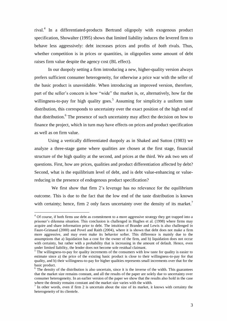
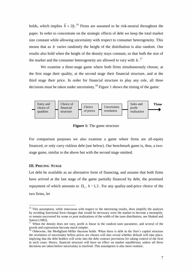
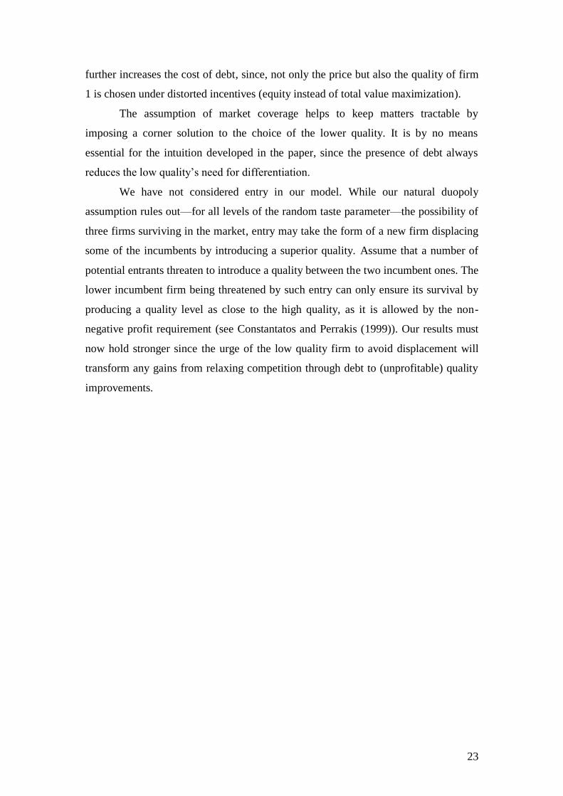
We examine a three-stage game where both firms simultaneously choose, at

the first stage their quality, at the second stage their financial structure, and at the

third stage their price. In order for financial structure to play any role, all three

decisions must be taken under uncertainty.18

Figure 1 shows the timing of the game:

Figure 1: The game structure

For comparison purposes we also examine a game where firms are all-equity

financed, or only carry riskless debt (see below). Our benchmark game is, thus, a two-

stage game, similar to the above but with the second stage omitted.

III. PRICING STAGE

Let debt be available as an alternative form of financing, and assume that both firms

have arrived at the last stage of the game partially financed by debt, the promised

repayment of which amounts to kD , 1,2k . For any quality-and-price choice of the

two firms, let

16

This assumption, while innocuous with respect to the interesting results, does simplify the analysis

by avoiding functional form changes that would be necessary were the market to become a monopoly,

or remain uncovered for some ex post realizations of the width of the taste distribution, see Shaked and

Sutton (1982). 17

When the density does not vary, profit is linear in the random taste parameter, and several of the

proofs and expressions become much simpler. 18

Otherwise, the Modigliani-Miller theorem holds. When there is debt in the firm’s capital structure

the revelation of uncertainty before prices are chosen will also reveal whether default will take place,

implying that the debt holders will write into the debt contract provisions for taking control of the firm

in such cases. Hence, financial structure will have no effect on market equilibrium, unless all three

decisions are taken before uncertainty is resolved. This assumption is also more realistic.

Choice

of prices

Entry and

choice of

qualities

Choice of

financial

structure

Uncertainty

revelation

Sales and

profit

realization

Time

8

1 1 1 1 11 ,B Bb t t ab p F u p F u

b a b a (3a)

2 2 2Bt a

b p F ub a

, (3b)

represent the operating profits of firms 1 and 2, respectively, at any realization of b.19

Then, 1D define 1zb D , and 2D define 2wb D such that

1 1zb D , and 2 2wb D . (4)

For any given quality-price choice the profit of firm 1 is increasing in ,b therefore zb

represents the lowest realization of the random variable that allows firm 1 to break-

even:20

firm 1 is solvent for ,zb b b and in default for zbbb , ; we denote zb the

default market size. From (4), an increase in 1D increases ceteris paribus zb , thus

increasing the bankruptcy interval , zb b and the cumulative probability of

bankruptcy. Let |z zb E b b b denote the truncated expectation of b conditional on

firm 1’s solvency. Our constant market size assumption requires that a larger width

corresponds to a thinner density, hence, the profit of firm 2 depends negatively on the

realization of b.21

The value of wb represents, therefore, the highest realization of the

random variable that allows firm 2 to break-even, that firm being solvent for

, wb b b and in default for ,wb b b .

Let 21

* ,; uubi , ,2,1i indicate the maximized profit of firm i for any given

realization of b known ex-ante with certainty.22

If 1

*

11 DbD , then bbz , so

that at any possible demand state firm 1 goes bankrupt. It is natural to assume that 1D

is an upper bound to the borrowing available to firm 1. On the other hand, when

1

*

11 DbD ,23

then bbz , implying that leverage induces no bankruptcy at any

19

Strictly speaking, we need to multiply the revenue part of (3a) and (3b) with a constant in order to

convert the shares of the constant market size of the two firms into sales; we normalize the constant to

1 without loss of generality. 20

From (1), the value of Bt depends only on prices and qualities which are chosen prior to uncertainty

resolution; hence, it is not stochastic 21

If the size of the market is allowed to vary with b the profit of firm 2 non-stochastic. This change

does not alter our results. 22

The value of ;* bi can be easily found in the literature, see for instance Tirole (1988), p.297.

23 It can be shown that 0*

1 b .

9

demand state (riskless debt); hence, zb b . Since riskless debt produces neither

agency cost nor strategic effects, the equilibrium with riskless debt is similar to the

benchmark case of firms being all-equity financed, so any reference to the former

includes also the latter and vice versa. Analogously, one can define an interval

2 2,D D such that any debt level within that interval is feasible and exposes firm 2 to

bankruptcy risk. As it turns out, firm 2’s leverage—whether riskless or bankruptcy-

inducing—has no relevance for the equilibrium outcome, implying that this interval is

not important for our analysis. Hereafter, the presence of z or w in a subscript

indicates the presence of bankruptcy-inducing debt in the financial structure of firm 1

or firm 2, respectively; when z (w) appears as subscript in a mathematical expectation,

the expectation is conditional on zbb ( wbb ). The presence of v in a subscript

indicates absence of bankruptcy-inducing leverage.

In the last stage, the manager-owner of a levered firm maximizes the firm’s

expected equity value izE , 1,2,i rather than its expected total value ˆ ˆ ˆiz iz izV E D .

The problem of firm 1 is

1

1 1 1 1

1 1ˆˆmax ( )

z

b

z z z z z Bp

zb

E b b D p t a dG bb a b a

, (5)

while that of firm 2 is

2

2 2 2 2

1 1ˆˆmax ( )wb

w w w w w Bp

wb

E b b D p t a dG bb a b a

. (6)

Setting 1

( )z zb E b bb a

, and defining 1( ) ( )z zb a b , the resulting

reaction functions are

1 21 2 ( )zp b u p (7)

and

2 11 2p a u p (8)

Note immediately that the best reply of firm 1 increases monotonically in 1D , while

that of firm 2 is unaffected by the presence of 2D . This asymmetry stems from the

fact that the two firms face different types of uncertainty: from (3ab) it is clear that

firm 1 faces uncertainty over both the width and the density of its market, whereas

10

firm 2 only faces uncertainty with respect to the latter.24

Since the presence and

magnitude of 2D have no effect on the equilibrium outcome, we assume, hereafter,

that firm 2 is all-equity financed, i.e., wb b . Define 1 2 3z z zX b b a ,

2 2 3z z zX b b a , 1ˆ 2 3z z zX b b a , and 2

ˆ 2 3z z zX b b a . Let

also ,i izX X b and ˆ ˆi izX X b , .2,1i Solving (7) and (8) simultaneously we

find equilibrium prices:

1 2ˆ; ,iz z izp b u u X u , 1, 2i , (9)

Holding qualities fixed, an increase in debt increases both prices. The consumer who

is indifferent between the two products at equilibrium prices is characterized by

3Bz z zt b b a (10)

In the benchmark game either both firms are all-equity financed, or only

riskless debt is allowed, therefore each firm decides its price by maximizing its total

value. Since the amount of debt that is paid back is constant across all realizations of

b and ,bbz bbw , maximizing total value at the last stage corresponds to

maximizing operating profit:

1

1 1 1 1

1max 1 ( ) 1 ( ) ( )B

B Bp

b tp E p t a E p t a b

b a b a (11a)

2

2 2 2max ( )BB

p

t ap E p t a b

b a (11b)

The reaction function of firm 2 remains unchanged from (8) while that of firm 1

becomes

1 21 2p b u p (12)

The expression in (12) is similar to the corresponding one in (7) except that

zb has been replaced by b . However, this is an important difference since the

latter is a parameter, while the former a decision variable determined at previous

stages of the game. Since positive amounts of debt imply zb b , debt shifts the

price reaction function of the leveraged firm and makes its response softer.25

Solving

(12) and (8), last-stage equilibrium prices 1vp in the benchmark game are also given

24

Firm 1 faces uncertainty over both the size and the heterogeneity (width of taste variability among its

clientele) of its market, while firm 2 faces uncertainty only over the former. 25

Recall that for 11 DD , ˆ ˆzb b , and changes in debt do not affect the reaction function.

11

by (8-11) with ˆ ˆiz iX X , implying that for given qualities leverage results in higher

prices. Under the same condition it can also be easily verified that

1 1 2 2z v z vp p p p , i.e., the levered firm 1 raises its price more than its rival does.

Similarly, with respect to the indifferent consumer we have

Bv B B z Bzt t b t b t , as expected, since the higher increase in firm 1’s

price reduces its relative market share at any realization of b. In terms of the

Fudenberg and Tirole (1984) zoology, debt acquisition corresponds to a puppy dog

strategy, similar to increasing product differentiation. Bankruptcy risk and product

differentiation are ―substitutes‖ in softening price competition in the sense that a

given level of equilibrium price can be targeted by various izX̂ and u levels.

Substituting last stage equilibrium prices from (8) into (4) and (3) we obtain,

as functions of debt and qualities, firm 1’s price-maximized equity,

1 1 11 1

ˆ ˆ3ˆ[1 ( )] 2 ( )2

z z zz z z z

z

X X XE u G b b X

b a,

the face value of its debt as a function of the default market size,

1 11 1 1

ˆ3ˆ ( ), 2( )

z zz

z

X XD X u F u

b a (13)

and its total firm-value,

1 21 1 1 1

11 ( ) 1 2

b

z

b

p pV p a dG b F u Y u F u

u b a, (14)

with 1

( ) 2ˆ2 1 ( )3

zz z

b aY b X b 1 1 1

ˆ ˆ ˆ( ) 3z zb X X X . In the riskless debt

case, total value is also given by (14) with 2

1ˆ2 ( )zY b b b X :

2

1 1 1 1 1ˆˆ ( ) ( )vV V D D b X u F u (15)

Finally, the last-stage equilibrium value of debt and total-value of firm 2 is

2

2 2 2 2 2ˆ ( )B

z z

t aV p E F u X u b F u

b a. (16)

It is clear from (14) and (16) that, while both firms’ total value is affected by the

financial structure of firm 1, firm 2’s financial structure is irrelevant. Nonetheless,

(16) is needed for the verification of the viability of that firm.

12

IV. EQUILIBRIUM

In stage 2 we concentrate on the determination of financial structure for firm 1. From

equation (14) it is clear that the optimal amount of debt is chosen implicitly, by

choosing the default market size zb . For given qualities equation (4) defines an

implicit function 1( )zb D , thus making zb the decision variable in the choice of

structure. Since only one firm’s potential bankruptcy has strategic effects—hence,

only that firm’s financial structure matters for the equilibrium outcome—the results

are not altered if either debt or zb is used as a choice variable for the high quality

producer, given the equilibrium relation 1( )zb D between the two.26

Thus, the criticism

of Frank and Le Pape (2008), and Haan and Toolsema (2008) against such

substitution of strategic variables, does not apply in our case.

Before proceeding with the determination of firm 1’s financial structure in our

duopoly context it is useful to examine that firm’s optimal structure if it were the sole

producer in the market, protected by some legal entry barrier. Under our natural

duopoly assumption over the width of the distribution, if a single quality is supplied

then the market remains uncovered. The last consumer purchasing the available

product is now m m mt p u , where the subscript m indicates the monopoly case.

Replacing Bt by mt in (5) and maximizing yields 11 2 ( )mz zp b u . The price-

maximized value of the monopolist is 1 1

( )1

2

zmz z

bV b u a b F u .

Letting ' 0z zb b , we find that

' 1 ' 1 0,mzz

z z

bVb a b

b b

since zb b . Thus, the value of the monopolist is reduced as zb increases,

implying that the optimal financial structure for the protected monopolist is the one

that does not result in default-inducing debt. In the absence of strategic interaction

with a rival, the advantage of leverage (BL effect) disappears, leaving only the agency

cost (JM effect).

26

We discuss this relation further on in this section.

13

Firm 1 chooses its financial structure by maximizing (14) with respect to zb ,

taking qualities as given. Maximizing (14) with respect to 1ˆ

zX yields the following

result:

Proposition 1: There exists a unique optimal default market size *

zb for the high

quality firm 1 that corresponds to a default-inducing amount of debt. If

1 1ˆ ˆ3 2zX b X , then the optimal structure contains both debt and equity

financing and *

zb is given by

* *

1 1ˆ ˆ3 2 6 4 0z zX X b b a ; (17)

if 1 1

ˆ ˆ3 2zX b X , then bbz*

(corner solution) and the optimal structure consists

of all-debt financing.27

Proof: Differentiating (14) for given qualities, 1 zdV db is proportional to

1 1ˆ

z zdY dX 1 1ˆ ˆ3 2 zX X ; setting the latter equal to zero reduces to

6 ( ) 4 ( ) 0zb b a . Since 0zb

, *

1ˆ

zX is increasing in zb , and equal to 1X̂ at

zb b , therefore there is a unique value of zb satisfying (17); if this value is in the

admissible interval ,b b then it defines from (14) the optimal default market size

and corresponding amount of debt. Otherwise, at zb b we have

1 1ˆ ˆ3 2zX b X

and the optimal structure is all-debt, QED.

In order to see the intuition of Proposition 1, we re-write

1 1 1 1 1ˆ ˆ ˆ ˆ2z z zdY dX X X X . (18)

Combining (9) and (15) we see that, in the absence of leverage, the expected sales of

firm 1 is proportional to 1X̂ . Any strategic effect that succeeds in increasing firm 1’s

equilibrium price by 1 unit, increases, therefore, its revenue by an amount

proportional to 1 1X̂ dp . Hence, the first term of the derivative in (18) represents the

marginal benefit from an increase in bankruptcy-inducing debt. Such debt, however,

27

The notion of an all-debt capital structure is a limit case, since it is not compatible with the

subsequent price-setting decision of firm 2, where price is chosen by maximizing the value of equity.

14

implies also an agency cost in the form of price distortion at the third stage. This

agency cost is proportional to the second term in (18) which is proportional to the

difference 1 1ˆ ˆ

zX X = 1

ˆ 1X r , where 1 1

ˆ ˆz zr b X X , with 0zr b , and

1br . Since r is monotonically increasing in the zbb ratio, it can be

interpreted as an index of relative bankruptcy risk. Hence, the agency cost is

proportional to the degree of bankruptcy risk. Since the second term is zero for the

unlevered firm and 1ˆ

zX is continuous on 1 1

ˆ ,X X , some positive amount of debt

will always be contained in the optimal financial structure. An interior solution

requires sufficient leverage so that the marginal cost of debt (2nd

term) becomes equal

to the (constant) marginal benefit of debt (1st term). If the range of the taste parameter

b is not sufficient to set the marginal agency cost equal to the marginal benefit of

debt, there is a corner solution.

An interesting feature deriving from Proposition 1 is that, while quality

choices affect equilibrium debt, they do not affect equilibrium bankruptcy risk. From

(17), the optimal value of r , *

1 1ˆ ˆmin 3 2, zr X b X , implying that *r depends

only on consumer tastes and the distribution of the random variable.28

Hence, the

optimal bankruptcy risk is like a parameter determined prior to the game. For any

qualities chosen at the first stage, debt simply adjusts to the necessary level in order to

set the ratio 1 1ˆ ˆ

zX X equal to *r . Note also that the optimal bankruptcy risk and

corresponding structure depend crucially on the shape of the distribution of the

random parameter b . At the end of the next section we provide a numerical example

with the same parameter values but two different distributions of b , one of which

yields a corner and the other an interior solution.

Since condition (17) determines the optimal default market size and risk of

bankruptcy (rather than the optimal amount of debt), we still need to determine

whether there exists a unique feasible amount of debt 11 1,D D D , corresponding to

the value of *

zb determined from Proposition 1. In the appendix it is shown that:

28

Recall that 1X̂ is a parameter, depending only on consumer tastes and the distribution of the random

variable. Thus, changes in 1ˆ

zX are equivalent to changes in r.

15

Lemma 1: When 1 1

ˆ ˆ3 2zX b X , a sufficient condition for *

zb to correspond to a

unique value 11

*

1 ,DDD is 6 4 ( ) 0z zb b a , *[ , ]z zb b b .29

When

1 1ˆ ˆ3 2zX b X , 1sign zD b is positive in an open neighborhood to the left of

b , implying that *

zb b corresponds to *

1 1D D .

We now turn to stage 1. Since qualities are chosen before financial structure,

they are decided by maximizing total firm value. However, since the optimal value of

zb is independent of qualities and depends only on parameters, optimal qualities can

be expressed as functions of zb . The high quality is decided by maximizing equation

(14)—or (15) for the riskless debt case—with respect to 1u , which yields

*

* * * 1

1 12

z

z z

Y bu u b F , (19)

with * * 1 2

1 1 1ˆ( ( ) )v zu u b F b X for the riskless case. With respect to 2u , we note

that the derivative of the RHS of (16) is proportional to

2

2 2 2 2ˆ ( ) 0zdV du X b F u . Since the width of the consumer distribution

always assures full market coverage, the profit maximizing 2u is obtained at the

minimum level consistent with At a . Since At decreases in 2u , the optimal 2u sets

At a , i.e., *

2 2 , , ,ju p a j z v with 2p replaced by (9), yielding

* * * * * 112 2 1

1

ˆ2

ˆ 2

z zz z z z

z z

b a X a Yu u b u b F

b a X a,

* * * 1 212 2 1 1

1

ˆ2 ˆ( )ˆv

b a X au u b u b F b X

b a X a. (20)

The equilibrium of this game is summarized as follows. Optimal qualities are

given by (19), (20) with *

1 1 1ˆ ˆ ˆmin 3 2 , ;z zX X X b the optimal financial structure

of firm 1 contains leverage * * 1

1 1 1ˆ

z z zD D X b , i.e., the necessary amount of debt for

(4) to hold at the equilibrium value of * * 1

1ˆ

z z zb X b , while the financial structure of

29

Note, however, that even if the condition in the Lemma is not satisfied the only problem that may

arise is that there may be from (13) more than one debt level corresponding to the optimal default

market size.

16

firm 2 is irrelevant, hence undetermined; optimal prices are given by (9) with the

appropriate substitutions. When debt-financing is unavailable, or available at very

limited amounts 11 DD , firm 1’s financial structure becomes irrelevant, as well, and

equilibrium qualities and prices are given by (20), (19) and (9) with 1

ˆzX replaced by

1X̂ . Equilibrium firm values * *

1 2ˆ ˆ, , , ,j jV V j z v are obtained by substituting optimal

qualities and *

1ˆ

zX or * * 1

2 2 1ˆ ˆ ˆ

z z z zX X X b into (14)-(16). The above described

equilibrium requires that both firms are active in the market. Since * *

1 2ˆ ˆ , , ,j jV V j z v

we assume at this point that *

2ˆ 0, , .jV j z v

30

V. COMPARATIVE STATICS: EQUILIBRIUM PRICES, DIFFERENTIATION AND FIRM

VALUE

In this section we perform comparative statics focusing mainly on the

comparison between the levered and the unlevered equilibrium. We start by

comparing equilibrium qualities in the two situations.

Proposition 2: When bankruptcy-inducing leverage is allowed at the second stage,

both equilibrium optimal quality levels are higher than they would have been had

firms been limited to default-free debt, or all-equity financing, i.e., * *

iz ivu u , 1, 2i .

Proof: It is easy to check that both (18) and (19) are increasing in 1ˆ

zX . Since

1 1ˆ ˆ

zX X , the convexity of )(uF implies **

iviz uu . QED.

This result is due to the fact that for any given qualities, debt increases both

prices. Thus, the anticipation of debt increases both firms’ marginal revenue from

quality improvements, shifting firm 1’s reaction function in the qualities space to the

right, and that of firm 2 upwards. From (19) the reaction function of the lower quality

is upward sloping, therefore, * *

1 1z vu u , and * *

2 2z vu u .

Hereafter, we restrict the form of the cost-of-quality function to i iF u u ,

1,2,i with 1 in order to satisfy the convexity requirement 0F . While being

30

In standard vertical differentiation models, such as this one, once the viability of firm 2 is assured,

that of firm 1 follows a fortiori.

17

sufficiently general in order to approximate most smooth convex functions, it allows

us to obtain well defined results.31

The size of the convexity factor turns out to be

significant for some of our results.

Before deriving the remaining results a technical point needs to be addressed.

The specification of the cost function requires that firm 2’s viability be investigated,

instead of simply assumed.32

Lemma 2: Under our demand-cost assumptions 2.3565 the low-quality firm is

viable in equilibrium for all admissible parameter values and all probability

distributions. For 1,2.3565 the viability of firm 2 is parameter- and distribution-

dependent, holding if

1

1 1 1 1

1 1

ˆ ˆ ˆ ˆ(3 )

ˆ ˆz z

z z

X a X X X

X a a X a.

Proof: See the appendix.

From Lemma 2 and its proof it becomes obvious that the scale factor does

not affect the viability of the low quality firm. Since it can also be shown not to affect

any of the results that follow, it is hereafter normalized to 1.

Equilibrium product differentiation can be expressed either as a quality ratio

*

2

*

1 jj uu , or as the difference * * * * * *

1 1 1 2 1ˆ ˆ ˆ, ; , ; , ;j j ju r X u r X u r X , vzj , ,

with 1*r in the riskless-debt case. The difference * *

1ˆ, ;ju r X is very important

since it constitutes a component of equilibrium prices and firm values.

Proposition 3: When leverage financing is available a) the optimal quality ratio

*

2

*

1 uu is lower compared to the case where equity (riskless leverage) is the only

source of financing for firm 1. b) Concerning *u , 2 ,

**

vz uu , while for

2,1 , i) when 23*r (interior solution to (17)),

**

vz uu , always, while ii) for

31

The frequently used function 2 2i iF u u is a special case of the above, with 1 2, 2 .

32 We are indebted to a referee for pointing this out. By ―viability” we mean ex ante positive expected

value in equilibrium. This should not be confused with ―solvency‖, which describes whether in

equilibrium the ex post pay-offs are able to repay each firm’s debt. Recall that the low-quality firm’s

expected total value is independent of that firm’s leverage, while this is obviously untrue for its

solvency.

18

* 32

r (100% leverage), 1

ˆ 1,2X such that 1

ˆ ,X with 1X̂ ,

**

vz uu .

Proof: See the appendix.

The above result shows that product differentiation may increase only when

there is a corner solution of 100% debt and the value of is sufficiently close to 1.

For all but the lowest admissible values of the parameter in our cost function—

including 2 , as in the commonly used function 221 uuF —debt reduces

product differentiation for all market size parameters. Debt affects product

differentiation in two different ways. The first one is related to the BL effect, which

tends to raise both qualities by increasing the marginal revenue from quality

increments. This BL effect, however, has an ambiguous overall impact on

differentiation, since on the one hand the increase in marginal revenue is higher for

the high quality, but on the other hand the convexity of the cost function implies that

any given increase in marginal revenue translates into a more important increase of

the low quality. It turns out that, unless the cost function is very flat ( has values

below 2), the BL effect tends to reduce product differentiation. In addition, debt also

affects differentiation because, from (12), the two are substitutes in achieving any

given level of equilibrium prices. For sufficiently high degrees of convexity (at

least 2 ) both the BL effect and the substitution effect work towards reducing

differentiation.

Next, we examine the effect of debt on prices, which has three components.

The first operates through distorting the objective of the decision maker at the last

stage. This effect induces a softer reaction of the leveraged firm (BL effect), which in

turn results in, ceteris paribus, higher prices for both products.

The second component operates through the increase in qualities and also

tends to increase prices, since, ceteris paribus, consumers are willing to pay higher

prices for higher qualities (quality effect). The third effect of debt on prices operates

through the impact of debt on product differentiation and has the opposite direction: a

reduced u implies, ceteris paribus, stiffer price competition and lower prices

(reduced-differentiation effect). The next result (proven in the appendix) shows that

the BLS and quality effects together dominate the reduced-differentiation effect.

19

Proposition 4: In the presence of bankruptcy-inducing debt in the financial structure

of firm 1, both equilibrium prices are higher than in the case where firm 1 is

unlevered.33

Proof: See the appendix.

What was shown by equation (9) and the discussion surrounding equation (12)

for given qualities (short run) turns out to hold even when qualities adjust to their

equilibrium level (long run). The fact that prices go up is good news for the two firms,

but does not account for the entire story, since in equilibrium qualities are higher, and

therefore their production requires higher fixed cost. Thus, while leverage enhances

short-run profitability, exactly as in Showalter (1995), its long-run impact on firm

value is ambiguous. We analyze next the impact of debt on firm 1’s value and obtain

a rather surprising result, given the fact that debt makes a firm less aggressive and

competition is in strategic complements.

Proposition 5: 11 DD the value of firm 1 is a decreasing function of debt, with * *

1 1v zV V , the equilibrium value of the all-equity (riskless) firm.

Proof: See the appendix.

Proposition 5, which is a central result of this paper, has a striking feature: the

strategic use of two instruments, each of them known to relax price competition and

increase firm value, has the exact opposite result. This happens because by relaxing

price competition debt reduces firm 2’s need for differentiation and allows that firm to

bring the quality level of its product closer to that of firm 1’s. By doing so, firm 2

mitigates the effect of debt on price competition. Firm 1 sells now at a price which is

higher relative to the unlevered scenario, but not sufficiently so as to compensate for

the increased fixed cost of its product. Hence, when quality choices are endogenous, it

is optimal for the high quality firm to opt for an all-equity structure, or to only carry

riskless debt. This argument is illustrated by writing:

* * * * * * *

1 1 1 1 1 2 1

1 2 1

z z z z z z zdV V V du V du dudY

dr Y dr u dr u du dr (21)

33

The proof with respect to the low quality price holds for any cost of quality function.

20

The envelope theorem implies that at the optimal choice of 1u the second term

of (21) is zero. Assume for the sake of the argument that the financial decision at the

second stage yields an interior solution, implying that the first term is also zero.34

The

third term is negative: its first component is negative, since an increase in 2u , with

fixed 1u , implies a reduction in product differentiation; its second component is

positive since the quality reaction function of firm 2 has positive slope; its third

component has been shown to be positive in Proposition 2. Clearly, the negativity of

*

1zdV dr is due to the fact that firm 1’s leverage induces firm 2 to upgrade its

quality.35

Note also that fixing both qualities at their unlevered equilibrium levels

would have resulted in *

1 0zdV dr , since the second term of (21) would become

positive ( * *

1 1v zu u ), and the third, zero. This implies that when products are

differentiated, some amount of leverage increases the value of the levered firm (as in

Showalter (1995)), but only as long as the rival’s quality is exogenous. When the

reaction of rival quality to changes in debt is taken into account debt on the one hand

is no longer profitable, but on the other hand cannot be avoided in the absence of a

firm commitment on the part of firm 1 not to choose a levered financial structure once

qualities have been irreversibly fixed.

Despite the optimality of an all-equity structure, we know from Proposition 1

that in equilibrium firm 1 is levered. The reason is that, since * 1r and depends only

upon parameter values, qualities during the first stage are decided upon the

expectation that later on in the game (2nd

stage) firm 1 will take up some debt. Hence,

firm 2 chooses its quality expecting (correctly) that, no matter its choice, at the next

stage its rival will take up the necessary amount of leverage in order to reach *r .

Having assured a softer price reaction from its rival due to debt, firm 2 increases its

quality to a level *

2 zu above *

2vu , causing at the same time a reduction in the total-

value of firm 1.

The following conclusions emerge from the entire game. First, for given

qualities it is always optimal for the high quality producer to include debt in its

financial structure. Second, the availability of debt financing affects both quality

34

Proposition 5 holds even if the equilibrium financial structure is an all-debt one. The interior solution

assumption is used here just to present the intuition in a clearer and more concise manner. 35

The proof contained in the appendix shows that this result is not limited to the neighborhood of the

interior solution, but holds for all admissible values of the parameters.

21

choices upwards, despite the fact that qualities are decided before the financial

structure. Third, the availability of debt financing reduces product differentiation.

Fourth, despite the reduction in product differentiation, debt leads to higher prices for

both products. Fifth, the availability of debt reduces the value of firm 1.

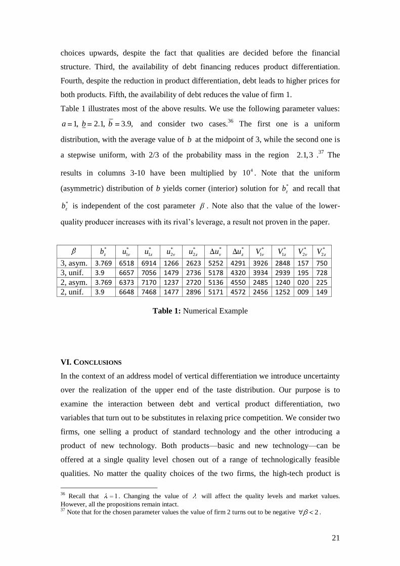
Table 1 illustrates most of the above results. We use the following parameter values:

1, 2.1, 3.9,a b b and consider two cases.36

The first one is a uniform

distribution, with the average value of b at the midpoint of 3, while the second one is

a stepwise uniform, with 2/3 of the probability mass in the region 2.1,3 .37

The

results in columns 3-10 have been multiplied by 410 . Note that the uniform

(asymmetric) distribution of b yields corner (interior) solution for *

zb and recall that

*

zb is independent of the cost parameter . Note also that the value of the lower-

quality producer increases with its rival’s leverage, a result not proven in the paper.

*

zb

*

1vu *

1zu *

2vu *

2zu *

vu

*

zu

*

1vV *

1zV *

2vV *

2zV

3, asym. 3.769 6518 6914 1266 2623 5252 4291 3926 2848 157 750

3, unif. 3.9 6657 7056 1479 2736 5178 4320 3934 2939 195 728

2, asym. 3.769 6373 7170 1237 2720 5136 4550 2485 1240 020 225

2, unif. 3.9 6648 7468 1477 2896 5171 4572 2456 1252 009 149

Table 1: Numerical Example

VI. CONCLUSIONS

In the context of an address model of vertical differentiation we introduce uncertainty

over the realization of the upper end of the taste distribution. Our purpose is to

examine the interaction between debt and vertical product differentiation, two

variables that turn out to be substitutes in relaxing price competition. We consider two

firms, one selling a product of standard technology and the other introducing a

product of new technology. Both products—basic and new technology—can be

offered at a single quality level chosen out of a range of technologically feasible

qualities. No matter the quality choices of the two firms, the high-tech product is

36

Recall that 1 . Changing the value of will affect the quality levels and market values.

However, all the propositions remain intact. 37

Note that for the chosen parameter values the value of firm 2 turns out to be negative 2 .

22

always viewed as superior quality by consumers (no leapfrogging). Both firms choose

their quality level simultaneously (no incumbent-entrant relations). We assume that,

while the low end of the consumer taste distribution is known with certainty, the

position of the high end is uncertain and only its distribution is known. This implies

that the two firms face an asymmetric situation: while the willingness-to-pay for

quality improvements of the standard product is known, the corresponding one for a

new-technology product is uncertain. After specifying their product and before

announcing their price, both firms can underwrite debt.

Since the lower quality faces uncertainty only with respect to the density of its

market, its debt is of no importance for the equilibrium outcome. On the contrary, the

high quality is always levered in equilibrium and its leverage has the following

important consequences for the equilibrium outcome. First, in anticipating leverage,

both firms increase their quality. Second, except for a small set of admissible

parameters determined in the text, debt reduces equilibrium product differentiation.

Knowing that its rival will be levered, the low quality firm expects softer price

competition, for any product specification. Hence, it chooses a product quality that, in

the absence of debt, would have been unprofitable due to triggering very stiff price

competition. Third, despite reduced differentiation, long-run equilibrium prices are

higher, compared to situations where firm 1 uses only equity financing. Fourth,

despite the higher prices, the value of the high quality firm is reduced, compared to

the case of all-equity financing. The fall in the value of the high quality firm is due to

the upgrading of the lower quality. This conclusion is in sharp contrast with short-run

analysis where qualities are given and debt enhances the total value of the high quality

firm. Even if leverage is value-reducing, the high quality firm cannot commit to all-

equity financing because after qualities have been chosen, it becomes rational to

include debt in its financial structure.

The above conclusions are robust if one allows the market size to vary

together with consumer heterogeneity. In such a case the height of the density remains

constant even though its width changes with the parameter b. The results of this case

are virtually identical to the ones in this paper. Some of the conclusions are also

robust to altering the decision sequence so that the financial decision precedes the

choice of quality, as shown in a companion paper (see Constantatos and Perrakis,

2010). In fact, the prior choice of leverage induces a second agency distortion that

23

further increases the cost of debt, since, not only the price but also the quality of firm

1 is chosen under distorted incentives (equity instead of total value maximization).

The assumption of market coverage helps to keep matters tractable by

imposing a corner solution to the choice of the lower quality. It is by no means

essential for the intuition developed in the paper, since the presence of debt always

reduces the low quality’s need for differentiation.

We have not considered entry in our model. While our natural duopoly

assumption rules out—for all levels of the random taste parameter—the possibility of

three firms surviving in the market, entry may take the form of a new firm displacing

some of the incumbents by introducing a superior quality. Assume that a number of

potential entrants threaten to introduce a quality between the two incumbent ones. The

lower incumbent firm being threatened by such entry can only ensure its survival by

producing a quality level as close to the high quality, as it is allowed by the non-

negative profit requirement (see Constantatos and Perrakis (1999)). Our results must

now hold stronger since the urge of the low quality firm to avoid displacement will

transform any gains from relaxing competition through debt to (unprofitable) quality

improvements.

24

References

Brander James A., and Tracy R. Lewis, "Oligopoly and Financial Structure: The Limited

Liability Effect", American Economic Review, 76 (1986), 956-970.

Calveras, Aleix, Juan-Jose Ganuza, and Esther Hauk, ―Wild Bids. Gambling for

Resurrection in Procurement Contracts‖ Journal of Regulatory Economics, 26:1,

(2004), 41-68.

Chevalier, J. A., "Do LBO Supermarkets Charge More? An Empirical Analysis of the

Effects of LBOs on Supermarket Pricing", Journal of Finance, 50 (1995), 1095-

1112.

Chevalier, J. A., and D. Scharfstein, "Capital Market Imperfections and Countercyclical

Markups: Theory and Evidence", American Economic Review, 86 (1996), 703-

725.

Constantatos, Christos and S. Perrakis, "Vertical Differentiation: Entry and Market

Coverage with Multiproduct Firms", International Journal of Industrial

Organization, 16 (1997), 81-103.

Constantatos, Christos, and S. Perrakis, "Free Entry May Reduce Total Willigness-to-

Pay", Economic Letters, 62, (1999), 105-112.

Constantatos, Christos, and S. Perrakis, "On the Impact of Financial Structure on

Product Selection", Discussion Paper Series No 2010_11, Department of

Economics, University of Macedonia, (2010).

Dasgupta, Sudipto, and Sheridan Titman, "Pricing Strategy and Financial Policy",

Review of Financial Studies, 11 (1998), 705-737.

Faure-Grimaud, Antoine, ―Product Market Competition and Optimal Debt Contracts: the

Limited Liability Effect Revisited‖, European economic Review, 44 (2000),

1823-1840.

Fudenberg, Drew, and J. Tirole, ―The Fat-Cat Effect, the Puppy Dog Ploy and the Lean

and Hungry Look‖, American Economic Review, 74 (1984), 361-366.

Gabszewicz, Jaskold-J., and J.-F. Thisse, "Entry (and Exit) in a Differentiated Industry",

Journal of Economic Theory, 22 (1980), 327-338.

Garella, Paolo G., and Emmanuel Petrakis, "Minimum Quality Standards and

Consumers’ Information", Economic Theory, 36 (2008), 283-302.

Haan, Marco A., and Linda A. Toolsema, ―The Strategic Use of Debt Reconsidered.‖

International Journal of Industrial Organization, 26, (2008), 616-624.

Harris, M., and A. Raviv, "The Theory of Capital Structure", Journal of Finance, 46

(1991), 297-355.

25

Hughes, John S., Jennifer L. Kao, and Arijit Mukherji, ―Oligopoly, Financial Structure

and Resolution of Uncertainty.‖ Journal of Economics and Management

Strategy, 7:1, (1998), 67-88.

Jensen, M. C., and W. H. Meckling, ―Theory of the Firm: Managerial Behavior, Agency

Costs and Ownership Structure‖, Journal of Financial Economics, 3, (1976),

305-360.

Jensen, Richard, and Dean Showalter, ―Strategic Debt and Patent Races‖, International

Journal of Industrial Organization, 22:7, (2004), 887-915.

Franck, Bernard and Nicolas Le Pape, ―The Commitment Value of the Debt: A

Reappraisal.‖ International Journal of industrial Organization, 26, (2008), 607-

615.

Lyandres, Evgeny, ―Capital Structure and Interaction Among Firms in Output Markets:

Theory and Evidence‖, Journal of Business, 79, (2006), 2381-2421.

Lyandres, Evgeny, ―Strategic Cost of Diversification‖, Review of Financial Studies, 20

(2007), 1901-1940.

Maksimovic, Vojislav, "Capital Structure in Repeated Oligopolies", Rand Journal of

Economics, 19 (1988), 389-447.

Maksimovic, V., and S. Titman, "Financial Reputation and Reputation for Product

Quality", Review of Financial Studies, 4 (1991), 175-200.

Modigliani, M., and Merton Miller, "The Cost of Capital, Corporate Finance, and the

Theory of Investment", American Economic Review 48 (1958), 261-297.

Motta M., J.F. Thisse, and A. Cabrales, ―On the Persistence of Leadership of

Leapfrogging in International Trade‖, International Economic Review, 38

(1997), 809-824.

Phillips, G, "Increased Debt and Product Market Competition: an Empirical Analysis",

Journal of Financial Economics, 37 (1994), 189-238.

Poitevin, Michel, "Collusion and the Banking Structure of a Duopoly", Canadian

Journal of Economics, 22 (1989), 263-277.

Povel, Paul, and Michael Raith, ―Financial Constraints and Product Market Competition:

ex ante vs. ex post Incentives.‖ International Journal of Industrial

Organization, 22 (2004), pp 917-949.

Shaked, Avner and J. Sutton, "Relaxing Price Competition Through Product

Differentiation", Review of Economic Studies, 44 (1982), 3-13.

Shaked, Avner and J. Sutton, "Natural Oligopolies", Econometrica, 51 (1983), 1469-

1484.

Showalter, Dean M., "Oligopoly and Financial Structure: Comment", American

Economic Review, 85 (1995), 647-653.

26

Showalter, Dean, "Strategic Debt: Evidence in Manufacturing", International Journal of

Industrial Organization, 17:3 (1999a), 299-318.

Showalter, Dean, "Debt as an Entry Deterrent under Bertrand Price Competition",

Canadian Journal of Economics / Révue Canadienne d’Économique, 32:4

(1999b), 1069-1081.

Tirole, Jean, The Theory of Industrial Organization, MIT Press, 1988.

Wanzenried, Gabrielle, "Capital Structure Decisions and Output Market Competition

under Demand Uncertainty", International Journal of Industrial Organization,

21 (2003), 171-200.

27

Appendix:

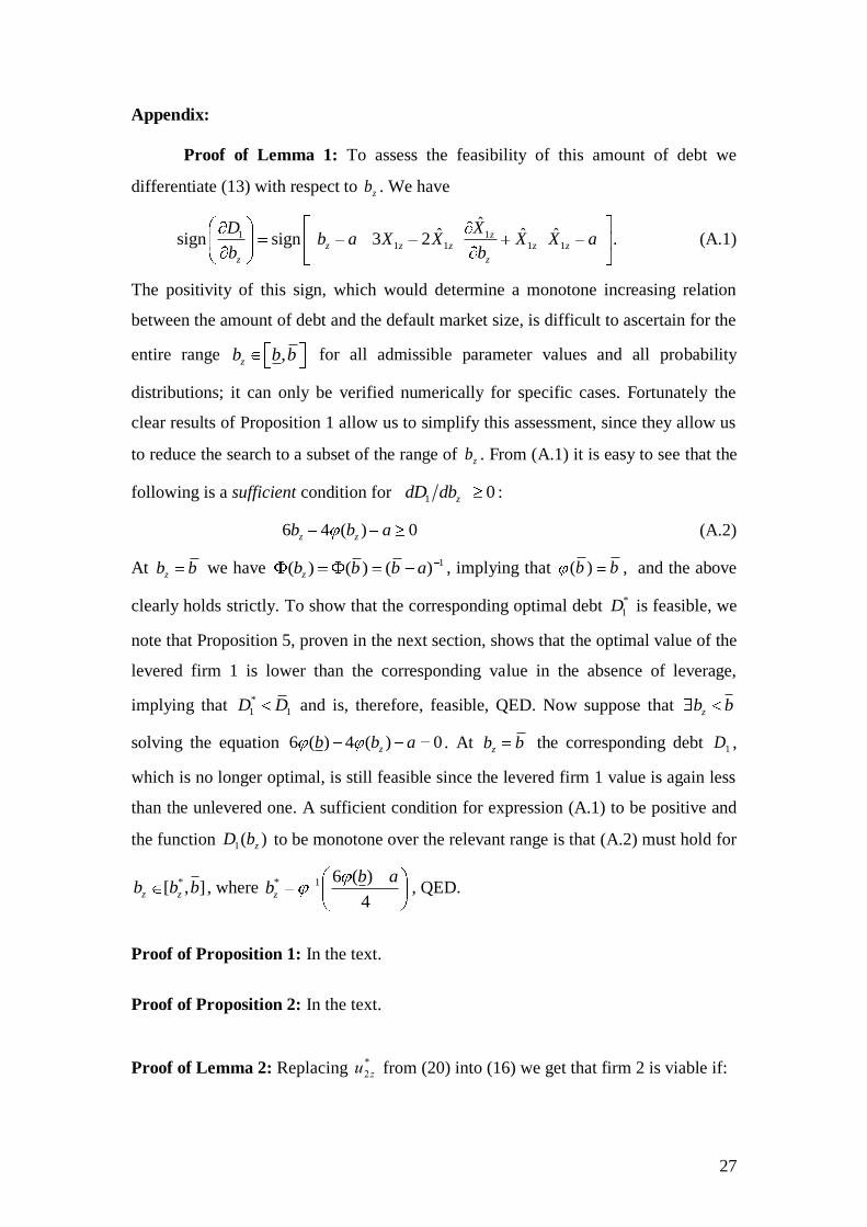
Proof of Lemma 1: To assess the feasibility of this amount of debt we

differentiate (13) with respect to zb . We have

1 11 1 1 1

ˆˆ ˆ ˆsign sign 3 2 .z

z z z z z

z z

D Xb a X X X X a

b b (A.1)

The positivity of this sign, which would determine a monotone increasing relation

between the amount of debt and the default market size, is difficult to ascertain for the

entire range ,zb b b for all admissible parameter values and all probability

distributions; it can only be verified numerically for specific cases. Fortunately the

clear results of Proposition 1 allow us to simplify this assessment, since they allow us

to reduce the search to a subset of the range of zb . From (A.1) it is easy to see that the

following is a sufficient condition for 1 0zdD db :

6 4 ( ) 0z zb b a (A.2)

At zb b we have 1( ) ( ) ( )zb b b a , implying that ( )b b , and the above

clearly holds strictly. To show that the corresponding optimal debt *

1D is feasible, we

note that Proposition 5, proven in the next section, shows that the optimal value of the

levered firm 1 is lower than the corresponding value in the absence of leverage,

implying that *

1 1D D and is, therefore, feasible, QED. Now suppose that zb b

solving the equation 6 ( ) 4 ( ) 0zb b a . At zb b the corresponding debt 1D ,

which is no longer optimal, is still feasible since the levered firm 1 value is again less

than the unlevered one. A sufficient condition for expression (A.1) to be positive and

the function 1( )zD b to be monotone over the relevant range is that (A.2) must hold for

*[ , ]z zb b b , where * 1 6 ( )

4z

b ab , QED.

Proof of Proposition 1: In the text.

Proof of Proposition 2: In the text.

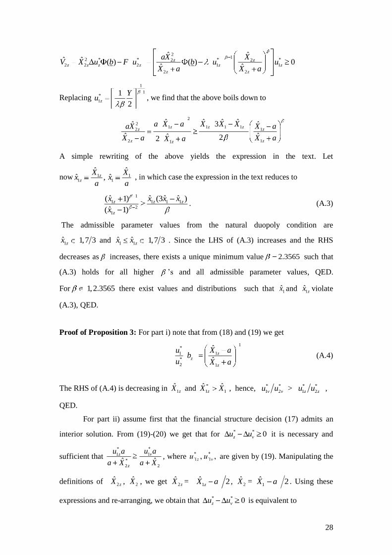
Proof of Lemma 2: Replacing *

2 zu from (20) into (16) we get that firm 2 is viable if:

28

21

2 * * * *2 22 2 2 1 1

2 2

ˆ ˆˆ ˆ ( ) ( ) 0

ˆ ˆz z

z z z z z z

z z

aX XV X u b F u b u u

X a X a

Replacing

1

1*

1

1

2z

Yu , we find that the above boils down to

2

21 1 1 1

2 1

2 11

ˆ ˆ ˆ ˆ3ˆ ˆ

ˆ ˆˆ 22

z z zz z

z zz

a X a X X XaX X a

X a X aX a

A simple rewriting of the above yields the expression in the text. Let

now 1 11 1

ˆ ˆˆ ˆ, z

z

X Xx x

a a , in which case the expression in the text reduces to

1

1 1 1 1

2

1

ˆ ˆ ˆ ˆ( 1) (3 )

ˆ( 1)z z z

z

x x x x

x. (A.3)

The admissible parameter values from the natural duopoly condition are

1̂ 1,7 3zx and 1 1ˆ ˆ 1,7 3zx x . Since the LHS of (A.3) increases and the RHS

decreases as increases, there exists a unique minimum value 2.3565 such that

(A.3) holds for all higher ’s and all admissible parameter values, QED.

For 1,2.3565 there exist values and distributions such that 1x̂ and 1̂zx violate

(A.3), QED.

Proof of Proposition 3: For part i) note that from (18) and (19) we get

1*

1 1

*

2 1

ˆ

ˆz

z

z

u X ab

u X a (A.4)

The RHS of (A.4) is decreasing in 1ˆ

zX and *

1 1ˆ ˆ

zX X , hence, * *

1 2v vu u > * *

1 2z zu u ,

QED.

For part ii) assume first that the financial structure decision (17) admits an

interior solution. From (19)-(20) we get that for * * 0z vu u it is necessary and

sufficient that **

11

*

2 2ˆ ˆ

vz

z

u au a

a X a X, where ,, *

1̀

*

1̀ vz uu are given by (19). Manipulating the

definitions of 2ˆ

zX , 2X̂ , we get 2ˆ

zX = 1

ˆ 2zX a , 2X̂ =1

ˆ 2X a . Using these

expressions and re-arranging, we obtain that * * 0z vu u is equivalent to

29

1 *

1

* 1 2

1 1

ˆ2

ˆ ˆ

z

z

F Y b a X

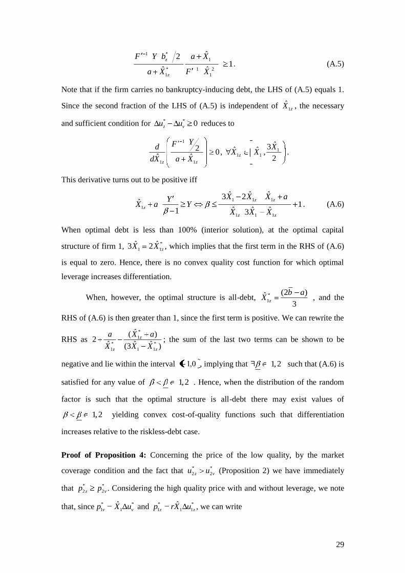
a X F X 1. (A.5)

Note that if the firm carries no bankruptcy-inducing debt, the LHS of (A.5) equals 1.

Since the second fraction of the LHS of (A.5) is independent of 1

ˆzX , the necessary

and sufficient condition for * * 0z vu u reduces to

1

1 1

20

ˆ ˆz z

YFd

dX a X, 1

1 1

ˆ3ˆ ˆ ,2

z

XX X .

This derivative turns out to be positive iff

1 1 1

1

1 1 1

ˆ ˆ ˆ3 2ˆ 1

ˆ ˆ ˆ1 3

z z

z

z z

X X X aYX a Y

X X X. (A.6)

When optimal debt is less than 100% (interior solution), at the optimal capital

structure of firm 1, *

1 1ˆ ˆ3 2 zX X , which implies that the first term in the RHS of (A.6)

is equal to zero. Hence, there is no convex quality cost function for which optimal

leverage increases differentiation.

When, however, the optimal structure is all-debt, *

1

(2 )ˆ3

z

b aX , and the

RHS of (A.6) is then greater than 1, since the first term is positive. We can rewrite the

RHS as *

1

* *

1 1 1

ˆ( )2

ˆ ˆ ˆ(3 )

z

z z

X aa

X X X; the sum of the last two terms can be shown to be

negative and lie within the interval 0,1 , implying that 1,2 such that (A.6) is

satisfied for any value of 1,2 . Hence, when the distribution of the random

factor is such that the optimal structure is all-debt there may exist values of

1,2 yielding convex cost-of-quality functions such that differentiation

increases relative to the riskless-debt case.

Proof of Proposition 4: Concerning the price of the low quality, by the market

coverage condition and the fact that * *

2 2z vu u (Proposition 2) we have immediately

that * *

2 2z vp p . Considering the high quality price with and without leverage, we note

that, since* *

1 1ˆ

v vp X u and * *

1 1 1ˆ

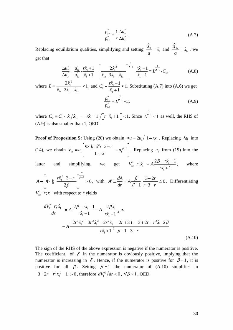
z zp rX u , we can write

30

* *

1

* *

1

1v v

z z

p u

p r u. (A.7)

Replacing equilibrium qualities, simplifying and setting 11

ˆˆ

Xx

a and 1

1

ˆˆz

z

Xx

a, we

get that 1

1* * 2 111 1 1 1

1* *

1 1 1 1 1 1

ˆ ˆ ˆ1 2 1

ˆ ˆ ˆ ˆ ˆ1 3 1

v v

z z z z

u u rx x rxL C

u u x x x x x, (A.8)

where 2

1

1 1 1

ˆ21

ˆ ˆ ˆ3z z

xL

x x x, and 1

1

1

ˆ 11

ˆ 1

rxC

x. Substituting (A.7) into (A.6) we get

1*

112*

1

v

z

pL C

p (A.9)

where 2 1 1 1 1 1

ˆ ˆ ˆ ˆ1 1 1zC C x x rx r x . Since

1

1 1L as well, the RHS of

(A.9) is also smaller than 1, QED.

Proof of Proposition 5: Using (20) we obtain 12 1u u rx . Replacing u into

(14), we obtain

2

1

1 1 1

ˆ 3

1z

b x r rV u u

rx. Replacing 1u from (19) into the

latter and simplifying, we get * 11 1

1

ˆ2 1ˆ;

ˆ 1z

rxV r x A

rx, where

2 11̂ 3

02

rx rA b , with

3 20

1 3

dA rA A

dr r r. Differentiating

*

1 ;zV r x with respect to r yields

*

1 1 1 1

2

1 1

3 2 2 2 2 2

1 1 1 1

2

1

ˆ; ˆ ˆ2 1 2

ˆ 1 ˆ 1

ˆ ˆ ˆ ˆ2 3 2 2 3 3 2 2

ˆ 1 1 3

dV r x rx xA A

dr rx rx

r x r x r x r r r xA

rx r

(A.10)

The sign of the RHS of the above expression is negative if the numerator is positive.

The coefficient of in the numerator is obviously positive, implying that the

numerator is increasing in . Hence, if the numerator is positive for 1 , it is

positive for all . Setting 1 the numerator of (A.10) simplifies to 2 2

13 2 1 0r r x , therefore 1 0QdV dr , 1 , QED.

31

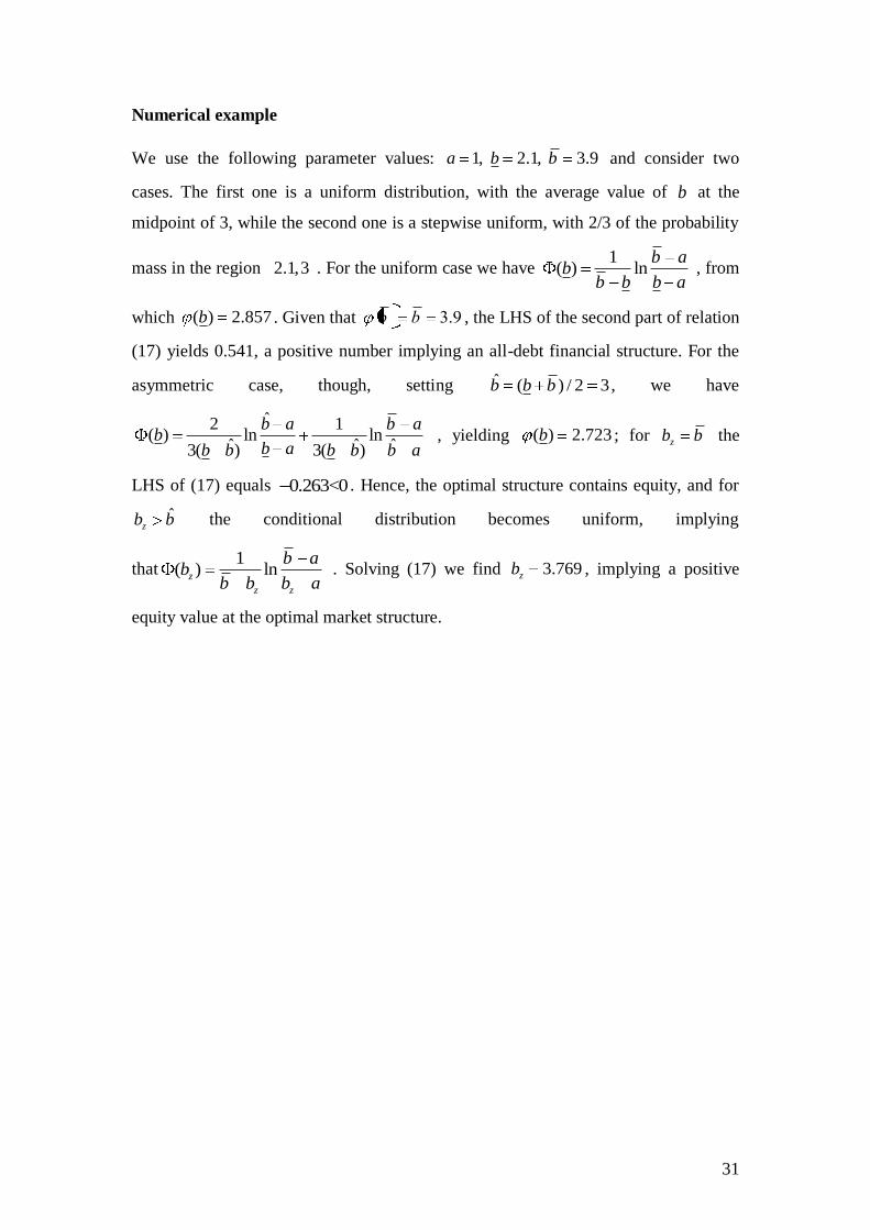
Numerical example

We use the following parameter values: 1, 2.1, 3.9a b b and consider two

cases. The first one is a uniform distribution, with the average value of b at the

midpoint of 3, while the second one is a stepwise uniform, with 2/3 of the probability

mass in the region 2.1,3 . For the uniform case we have 1

( ) lnb a

bb b b a

, from

which ( ) 2.857b . Given that 9.3bb , the LHS of the second part of relation

(17) yields 0.541, a positive number implying an all-debt financial structure. For the

asymmetric case, though, setting ˆ ( ) / 2 3b b b , we have

ˆ2 1( ) ln ln

ˆ ˆ ˆ3( ) 3( )

b a b ab

b ab b b b b a , yielding ( ) 2.723b ; for zb b the

LHS of (17) equals 0.263<0 . Hence, the optimal structure contains equity, and for

ˆzb b

the conditional distribution becomes uniform, implying

that1

( ) lnz

z z

b ab

b b b a . Solving (17) we find 3.769zb , implying a positive

equity value at the optimal market structure.