Energy-Represented Direct Inversion in the IterativeSubspace within a Hybrid Geometry Optimization Method

Xiaosong Li*

Department of Chemistry, UniVersity of Washington, Seattle, Washington 98195-1700

Michael J. Frisch

Gaussian, Inc., Wallingford, Connecticut 06492

Received November 8, 2005

Abstract: A geometry optimization method using an energy-represented direct inversion in the

iterative subspace algorithm, GEDIIS, is introduced and compared with another DIIS formulation

(controlled GDIIS) and the quasi-Newton rational function optimization (RFO) method. A hybrid

technique that uses different methods at various stages of convergence is presented. A set of

test molecules is optimized using the hybrid, GEDIIS, controlled GDIIS, and RFO methods.

The hybrid method presented in this paper results in smooth, well-behaved optimization

processes. The optimization speed is the fastest among the methods considered.

I. IntroductionGeometry optimization is an essential part of computationalchemistry. Any theoretical investigation that involves calcula-tions of transition structures, barrier heights, heats of reaction,or vibrational spectra requires searches for one or moreminima or saddle points on a potential energy surface (PES).Computational methods are applied to large systems of ever-increasing size. Biomolecules, polymers, and nanostructureswith hundreds to thousands of atoms are often difficult tooptimize because of excessive degrees of freedom. Anydecrease in the computational cost and increase in the generalstability of geometry optimization would be welcome.

A variety of algorithms for geometry optimization arewidely used in computational chemistry (for some recent re-views, see refs 1 and 2). Geometry optimization methodscan be broadly classified into two major categories. First-ordermethods use only analytic first derivatives to search for sta-tionary points; second-order methods use analytic first andsecond derivatives, assuming a quadratic model for the poten-tial energy surface and a Newton-Raphson step for theminima search

where g is the gradient (first derivative) andH-1 is theinverse Hessian (second derivative). While second-orderoptimization schemes need fewer steps to reach convergencethan first-order methods,3 this approach can quickly becomevery expensive with increasing system size because theexplicit computation of the Hessian scales asO(N4)-O(N5),where N is a measure of the system size. Quasi-Newtonmethods are intermediate between the first- and second-orderapproaches. An initial estimate of the Hessian is obtainedby some inexpensive method. Subsequently, the Hessian isupdated using the first derivatives and displacements, bymethods such as BFGS,4-7 SR1,8 and PSB.9,10 The quasi-Newton approach is comparable in computational cost tofirst-order methods and in convergence speed to second-ordermethods.

The use of a Newton-Raphson step when the PES is faraway from a quadratic region can lead to overly large stepsizes in the wrong direction. The stability of a Newton-Raphson geometry optimization can be enhanced by control-ling the step size using techniques such as rational functionoptimization (RFO)11,12 and the trust radius model.1-3,13-16

To reduce the number of iterations required to reachconvergence, a least-squares minimization scheme is used:direct inversion in the iterative subspace (DIIS).17,18The DIISapproach is efficient in both converging the wave function17-21

and optimizing the geometry.22,23It extrapolates/interpolatesa set of vectors{Ri} by minimizing the errors in the least-

* Corresponding author. Fax: 206-685-8665. E-mail: li@chem.washington.edu.

∆x ) -H-1g (1)

835J. Chem. Theory Comput.2006,2, 835-839

10.1021/ct050275a CCC: $33.50 © 2006 American Chemical SocietyPublished on Web 04/18/2006

squares sense (for a leading reference, see ref 17):

where λ is the Lagrangian multiplier. The coefficientsminimize a working function, which can be an errorfunction17,18,21-23 or an energy function.19,20Fock matrix andnuclear positions are often chosen as the vectors for self-consistent field (SCF)17,18,20,21and geometry22,23optimizations,respectively. When the working function is an error function,the matrix A is usually defined as the product of errorvectors,ai,j ) eiej

T, where the error vector can be a quasi-Newton step for geometry optimization22,23or the commutator[F, P] for SCF convergence.17,18 Solving eq 2 leads to a setof DIIS coefficientsci that are used to obtain a new vector,R* ) ∑iciRi, which has the minimum functional value withinthe search space. Direct solution of eq 2 often leads tounproductive oscillations when optimizing large systems.20,23

Farkas and Schlegel have introduced some controls to ensurea downhill DIIS extrapolation/interpolation for geometryoptimization (GDIIS).23 Scuseria and co-workers have in-troduced a stable and efficient alternative DIIS formalismfor SCF convergence, energy-DIIS (SCF-EDIIS).19,20 TheSCF-EDIIS algorithm minimizes an energy function andenforces coefficients to be positive definite.

This paper extends the energy-represented direct inversionin the iterative subspace algorithm from SCF convergenceto geometry optimization (GEDIIS). A hybrid geometryoptimization technique that utilizes the advantages of dif-ferent methods of various stages of the optimization is thenillustrated and tested.

II. Methodology and BenchmarksOptimizations are carried out using the development versionof the Gaussian series of programs24 with the addition ofthe geometry optimization algorithms using GEDIIS and thehybrid method presented here. For all methods, the geometryoptimization is considered converged when the root-mean-square (RMS) force is less than 1× 10-5 au, the RMSgeometry displacement is less than 4× 10-5 au, themaximum component of the force vector is less than 1.5×10-5 au, and the maximum component of the geometrydisplacement is less than 6× 10-5 au. All calculations arecarried out with redundant internal coordinates. No symmetryoperations or reorientations are imposed. Starting geometriesare available upon request (li@chem.washington.edu).

A. Geometry Optimization Using Energy-RepresentedDirect InVersion in the IteratiVe Subspace (GEDIIS).As inall DIIS-based schemes, the GEDIIS formalism yields a newvector R* constructed from a linear combination ofNpreviously computed vectorsRi

In GEDIIS,Ri’s are geometries andci’s minimize an energyfunction. The energy of the new structureR* can beapproximated to first order with an expansion atRi

whereE(Ri) andgi are the energy and gradient of structureRi, respectively. Multiplying both sides of eq 4 byci, andsumming overN points, we obtain

A simple algebraic manipulation leads to the GEDIISworking function

or

where

The quadratic term in eq 6 represents the variations in energyfor changes of geometric coordinates and gradients withinthe search space. Equation 6 is formally identical toScuseria’s SCF-EDIIS equation for wave-function optimiza-tion.20 In both the GEDIIS and SCF-EDIIS formalisms, theenergy function is minimized directly with respect to theexpansion coefficients,ci’s. The working functions in GE-DIIS, SCF-DIIS,17,18 SCF-EDIIS,20 and GDIIS22,23 are allquadratic with respect toci, and minimizations are thereforeperformed in a least-squares sense. The comparison of thistechnique with Pulay’s DIIS17,18 has been discussed exten-sively in the literature.19,20

The set of DIIS coefficients,ci’s, that minimize the energyfunction, eq 6, are used to construct a new geometryR*from a linear combination of known points (eq 3). Theresulting geometryR* is, to a first-order approximation,associated with the optimal energy within the search space.However,R* is not necessarily the final minimum structure.The distance fromR* to the minimum structure can beapproximated by a second-order Newton step. In this work,we use a RFO step for the second-order correction

where the parameterê is optimized using the RFO approach

A )(a1,1 ‚‚‚ a1,N 1l ‚‚‚ l l

aN,1 ‚‚‚ aN,N 11 ‚‚‚ 1 0)

(a1,1 ‚‚‚ a1,N 1l ‚‚‚ l l

aN,1 ‚‚‚ aN,N 11 ‚‚‚ 1 0)(c1

lcN

λ) ) (0l0

1) and∑ci ) 1 (2)

R* ) ∑i)1

N

ciRi, ∑i)1

N

ci ) 1 (3)

E(R* ) ) E(Ri) + (R* - Ri)gi (4)

E(R* ) ) ∑i)1

N

ci[E(Ri) + ∑j)1

N

cjRjgi - Rigi] (5)

E(R* ) )

∑i)1

N

ci E(Ri) -1

2∑i,j)1

N

cicj[Ri(gi - gj) + gi(Ri - Rj)] (6)

E(R* ) ) ∑i)1

N

ci E(Ri) -1

2∑i,j)1

N

cicj(gi - gj)(Ri - Rj)

∑i)1

N

ci ) 1

RN+1 ) R* + ∆R

) ∑i)1

N

ciRi - ∑i)1

N

cigi(H - ê)-1 (7)

836 J. Chem. Theory Comput., Vol. 2, No. 3, 2006 Li and Frisch

(note that the Hessian is a constant in a quadratic approxima-tion).11,12 With no constraint on the sign ofci, eq 7 isessentially an extrapolation; whenci > 0, it becomes aninterpolation step. When the molecular geometry is far fromconvergence, extrapolations can lead to erroneously largesteps away from the optimized geometry. To ensure opti-mization stability, an enforced interpolation constraint,ci >0, is added into eq 2 (for detailed machinery, see ref 20).As a result, GEDIIS searches for a new geometry in theregion close to the local potential energy surface, that is,interpolations only.

We update the geometric Hessian with first derivatives:a weighted combination of BFGS and SR123 with the squareroot of the Bofill25 weighting factor

Equation 8 has been successfully used for large-moleculegeometry optimization.26

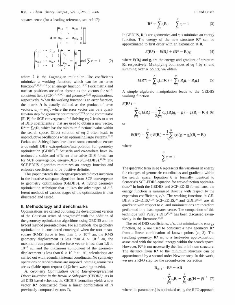
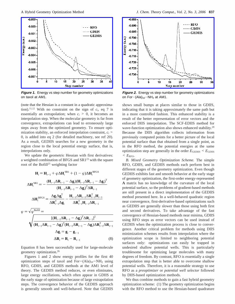
Figures 1 and 2 show energy profiles for the first 40optimization steps of taxol and For-(Ala)10-NH2 usingRFO, GDIIS, and GEDIIS methods at the AM1 level oftheory. The GEDIIS method reduces, or even eliminates,large energy oscillations, which often appear in GDIIS atthe early stage of optimization because of large extrapolationsteps. The convergence behavior of the GEDIIS approachis generally smooth and well-behaved. Note that GEDIIS

shows small bumps at places similar to those in GDIIS,indicating that it is taking approximately the same path butin a more controlled fashion. This enhanced stability is aresult of the better representation of error vectors and theenforced DIIS interpolation. The SCF-EDIIS method forwave-function optimization also shows enhanced stability.20

Because the DIIS algorithm collects information frompreviously computed points for a better picture of the localpotential surface than that obtained from a single point, asin the RFO method, the potential energies at the sameoptimization step are generally in the orderEGEDIIS < EGDIIS

< ERFO.B. Mixed Geometry Optimization Scheme.The simple

RFO, GDIIS, and GEDIIS methods each perform best indifferent stages of the geometry optimization. Even thoughGEDIIS exhibits fast and smooth behavior at the early stageof geometry optimization, the first-order energy-representedA matrix has no knowledge of the curvature of the localpotential surface, so the problems of gradient-based methodsare still present in a direct implementation of the GEDIISmethod presented here. In a well-behaved quadratic regionnear convergence, first-derivative-based optimizations suchas GEDIIS are generally slower than those using both firstand second derivatives. To take advantage of the fastconvergence of Hessian-based methods near minima, GDIISusing RFO steps as error vectors can be used instead ofGEDIIS when the optimization process is close to conver-gence. Another critical problem for methods using DIISminimization schemes results from interpolation where theoptimization scope is limited to neighboring potentialsurfaces only: optimizations can easily be trapped inundesired shallow potential wells. This is particularlytroublesome for optimizing large molecules with manydegrees of freedom. By contrast, RFO is essentially a singleextrapolation step that is better able to overcome shallowpotential wells. Therefore, it is a reasonable strategy to useRFO as apreoptimizeror potential well selectorfollowedby DIIS-based optimization methods.

We thus combine methods to gain a fast hybrid geometryoptimization scheme: (1) The geometry optimization beginswith the RFO method to use the Hessian-based quadrature

Figure 1. Energy vs step number for geometry optimizationson taxol at AM1.

H i ) H i-1 + æ∆H iSR1+ (1 - æ)∆H i

BFGS

∆H iSR1) -

(H i-1∆Ri-1 - ∆gi)(H i-1∆Ri-1 - ∆gi)T

(H i-1∆Ri-1 - ∆gi)T∆Ri-1

∆H iBFGS)

∆gi∆giT

∆Ri-1T ∆gi

-H i-1∆Ri-1∆Ri-1

T H i-1

∆Ri-1T H i-1∆Ri-1

æ ) xæBofill )

x [(H i-1∆Ri-1 - ∆gi)T∆Ri-1]

2

(H i-1∆Ri-1 - ∆gi)T(H i-1∆Ri-1 - ∆gi)∆Ri-1

T ∆Ri-1

∆gi ) gi - gi-1

∆Ri ) Ri - Ri-1 (8)

Figure 2. Energy vs step number for geometry optimizationson For-(Ala)10-NH2 at AM1.

A Hybrid Geometry Optimization Method J. Chem. Theory Comput., Vol. 2, No. 3, 2006837

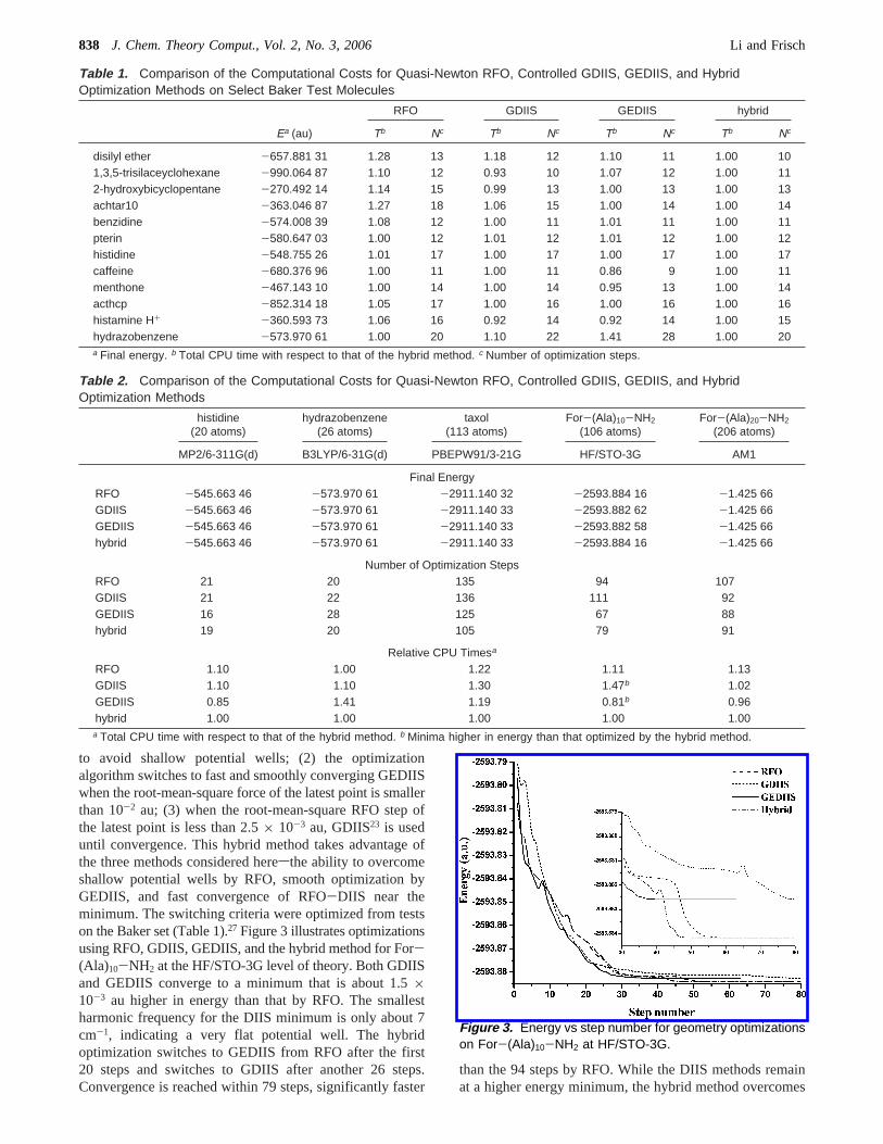
to avoid shallow potential wells; (2) the optimizationalgorithm switches to fast and smoothly converging GEDIISwhen the root-mean-square force of the latest point is smallerthan 10-2 au; (3) when the root-mean-square RFO step ofthe latest point is less than 2.5× 10-3 au, GDIIS23 is useduntil convergence. This hybrid method takes advantage ofthe three methods considered heresthe ability to overcomeshallow potential wells by RFO, smooth optimization byGEDIIS, and fast convergence of RFO-DIIS near theminimum. The switching criteria were optimized from testson the Baker set (Table 1).27 Figure 3 illustrates optimizationsusing RFO, GDIIS, GEDIIS, and the hybrid method for For-(Ala)10-NH2 at the HF/STO-3G level of theory. Both GDIISand GEDIIS converge to a minimum that is about 1.5×10-3 au higher in energy than that by RFO. The smallestharmonic frequency for the DIIS minimum is only about 7cm-1, indicating a very flat potential well. The hybridoptimization switches to GEDIIS from RFO after the first20 steps and switches to GDIIS after another 26 steps.Convergence is reached within 79 steps, significantly faster

than the 94 steps by RFO. While the DIIS methods remainat a higher energy minimum, the hybrid method overcomes

Table 1. Comparison of the Computational Costs for Quasi-Newton RFO, Controlled GDIIS, GEDIIS, and HybridOptimization Methods on Select Baker Test Molecules

RFO GDIIS GEDIIS hybrid

Ea (au) Tb Nc Tb Nc Tb Nc Tb Nc

disilyl ether -657.881 31 1.28 13 1.18 12 1.10 11 1.00 101,3,5-trisilaceyclohexane -990.064 87 1.10 12 0.93 10 1.07 12 1.00 112-hydroxybicyclopentane -270.492 14 1.14 15 0.99 13 1.00 13 1.00 13achtar10 -363.046 87 1.27 18 1.06 15 1.00 14 1.00 14benzidine -574.008 39 1.08 12 1.00 11 1.01 11 1.00 11pterin -580.647 03 1.00 12 1.01 12 1.01 12 1.00 12histidine -548.755 26 1.01 17 1.00 17 1.00 17 1.00 17caffeine -680.376 96 1.00 11 1.00 11 0.86 9 1.00 11menthone -467.143 10 1.00 14 1.00 14 0.95 13 1.00 14acthcp -852.314 18 1.05 17 1.00 16 1.00 16 1.00 16histamine H+ -360.593 73 1.06 16 0.92 14 0.92 14 1.00 15hydrazobenzene -573.970 61 1.00 20 1.10 22 1.41 28 1.00 20a Final energy. b Total CPU time with respect to that of the hybrid method. c Number of optimization steps.

Table 2. Comparison of the Computational Costs for Quasi-Newton RFO, Controlled GDIIS, GEDIIS, and HybridOptimization Methods

histidine(20 atoms)

hydrazobenzene(26 atoms)

taxol(113 atoms)

For-(Ala)10-NH2

(106 atoms)For-(Ala)20-NH2

(206 atoms)

MP2/6-311G(d) B3LYP/6-31G(d) PBEPW91/3-21G HF/STO-3G AM1

Final EnergyRFO -545.663 46 -573.970 61 -2911.140 32 -2593.884 16 -1.425 66GDIIS -545.663 46 -573.970 61 -2911.140 33 -2593.882 62 -1.425 66GEDIIS -545.663 46 -573.970 61 -2911.140 33 -2593.882 58 -1.425 66hybrid -545.663 46 -573.970 61 -2911.140 33 -2593.884 16 -1.425 66

Number of Optimization StepsRFO 21 20 135 94 107GDIIS 21 22 136 111 92GEDIIS 16 28 125 67 88hybrid 19 20 105 79 91

Relative CPU Timesa

RFO 1.10 1.00 1.22 1.11 1.13GDIIS 1.10 1.10 1.30 1.47b 1.02GEDIIS 0.85 1.41 1.19 0.81b 0.96hybrid 1.00 1.00 1.00 1.00 1.00

a Total CPU time with respect to that of the hybrid method. b Minima higher in energy than that optimized by the hybrid method.

Figure 3. Energy vs step number for geometry optimizationson For-(Ala)10-NH2 at HF/STO-3G.

838 J. Chem. Theory Comput., Vol. 2, No. 3, 2006 Li and Frisch

the shallow potential well and optimizes For-(Ala)10-NH2

to the RFO minimum.Table 2 compares final energies and computational costs

by the RFO, GDIIS, GEDIIS, and hybrid optimizationmethods on select molecules at various levels of theory. Thecomputational costs are presented as the relative CPU times.The hybrid method introduced in this paper is the fastestamong the popular geometry optimization methods consid-ered here. Most importantly, the optimization behavior ofthe hybrid method is consistently smooth and fast throughoptimizations of the Baker set and large biochemicalmolecules tested in this paper.

III. ConclusionThis paper presents a geometry optimization method usingGEDIIS. The GEDIIS method minimizes an energy repre-sentation of the local potential energy surface in the vicinityof previously computed points (gradients and geometries)as a least-squares problem. The enforced interpolation inGEDIIS leads to enhanced stability.

A hybrid geometry optimization algorithm is proposed thattakes into account the problems and advantages of differentoptimization methods. The hybrid method starts off withRFO as apreoptimizerand switches to GEDIIS when acertain convergence threshold is met. Near the minimum,GEDIIS switches to RFO-DIIS. This takes advantage ofRFO’s ability to overcome shallow potential wells, smoothoptimization by GEDIIS, and fast convergence of RFO-DIIS near the minimum. Optimizations of test molecules withthe hybrid method are shown to be smooth, reliable, and fast.

Acknowledgment. The authors are grateful for dis-cussions with Professor Schlegel at Wayne State University.

References

(1) Schlegel, H. B. Geometry Optimization on Potential EnergySurfaces. InModern Electronic Structure Theory; Yarkony,D. R., Ed.; World Scientific: Singapore, 1995; p 459.

(2) Schlegel, H. B. Geometry Optimization. InEncyclopedia ofComputational Chemistry; Schleyer, P. v. R., Allinger, N.L., Kollman, P. A., Clark, T., Schaefer, H. F., III, Gasteiger,J., Schreiner, P. R., Eds.; Wiley: Chichester, U. K., 1998;Vol. 2, p 1136.

(3) Fletcher, R.Practical Methods of Optimization; Wiley:Chichester, U. K., 1981.

(4) Broyden, C. G.J. Inst. Math. Appl.1970, 6, 76.

(5) Fletcher, R.Comput. J. (Switzerland)1970, 13, 317.

(6) Goldfarb, D.Math. Comput.1970, 24, 23.

(7) Shanno, D. F.Math. Comput.1970, 24, 647.

(8) Murtagh, B.; Sargent, R. W. H.Comput. J. (Switzerland)1972, 13, 185.

(9) Powell, M. J. D.Nonlinear Programing; Academic: NewYork, 1970.

(10) Powell, M. J. D.Math. Program.1971, 1, 26.

(11) Banerjee, A.; Adams, N.; Simons, J.; Shepard, R.J. Phys.Chem.1985, 89, 52.

(12) Simons, J.; Nichols, J.Int. J. Quantum Chem.1990, 24, 263.

(13) Murray, W.; Wright, M. H.Practical Optimization; Aca-demic: New York, 1981.

(14) Nonlinear Optimization; Powell, M. J. D., Ed.; Academic:New York, 1982.

(15) Dennis, J. E.; Schnabel, R. B.Numerical Methods forUnconstrained Optimization and Nonlinear Equations; Pren-tice Hall: Upper Saddle River, New Jersey, 1983.

(16) Scales, L. E.Introduction to Nonlinear Optimization; Mac-millam: Basingstoke, England, 1985.

(17) Pulay, P.Chem. Phys. Lett.1980, 73, 393.

(18) Pulay, P.J. Comput. Chem.1982, 3, 556.

(19) Cance`s, E.; Le Bris, C.Int. J. Quantum Chem.2000, 79,82.

(20) Kudin, K. N.; Scuseria, G. E.; Cance`s, E. J. Chem. Phys.2002, 116, 8255.

(21) Li, X.; Millam, J. M.; Scuseria, G. E.; Frisch, M. J.; Schlegel,H. B. J. Chem. Phys.2003, 119, 7651.

(22) Csaszar, P.; Pulay, P.J. Mol. Struct.1984, 114, 31.

(23) Farkas, O¨ .; Schlegel, H. B.Phys. Chem. Chem. Phys.2002,4, 11.

(24) Frisch, M. J.; Trucks, G. W.; Schlegel, H. B.; Scuseria, G.E.; Robb, M. A.; Cheeseman, J. R.; Montgomery, J. A., Jr.;Vreven, T.; Kudin, K. N.; Burant, J. C.; Millam, J. M.;Iyengar, S. S.; Tomasi, J.; Barone, V.; Mennucci, B.; Cossi,M.; Scalmani, G.; Rega, N.; Petersson, G. A.; Ehara, M.;Toyota, K.; Hada, M.; Fukuda, R.; Hasegawa, J.; Ishida, M.;Nakajima, T.; Kitao, O.; Nakai, H.; Honda, Y.; Nakatsuji,H.; Li, X.; Knox, J. E.; Hratchian, H. P.; Cross, J. B.; Adamo,C.; Jaramillo, J.; Cammi, R.; Pomelli, C.; Gomperts, R.;Stratmann, R. E.; Ochterski, J.; Ayala, P. Y.; Morokuma,K.; Salvador, P.; Dannenberg, J. J.; Zakrzewski, V. G.;Dapprich, S.; Daniels, A. D.; Strain, M. C.; Farkas, O.;Malick, D. K.; Rabuck, A. D.; Raghavachari, K.; Foresman,J. B.; Ortiz, J. V.; Cui, Q.; Baboul, A. G.; Clifford, S.;Cioslowski, J.; Stefanov, B. B.; Liu, G.; Liashenko, A.;Piskorz, P.; Komaromi, I.; Martin, R. L.; Fox, D. J.; Keith,T.; Al-Laham, M. A.; Peng, C. Y.; Nanayakkara, A.;Challacombe, M.; Gill, P. M. W.; Johnson, B.; Chen, W.;Wong, M. W.; Gonzalez, C.; Pople,J. A. DeVelopmentVersion ReV. D01 ed.; Gaussian, Inc.: Pittsburgh, PA, 2005.

(25) Bofill, J. M. J. Comput. Chem.1994, 15, 1.

(26) Farkas, O¨ .; Schlegel, H. B.J. Chem. Phys.1999, 111, 10806.

(27) Baker, J.J. Comput. Chem.1993, 14, 1085.

CT050275A

A Hybrid Geometry Optimization Method J. Chem. Theory Comput., Vol. 2, No. 3, 2006839