ENGG2450 Probability and Statistics for EngineersENGG2450 Probability and Statistics for Engineers

1 Introduction3 Probability3 Probability4 Probability distributions5 Probability Densities5 Probability Densities2 Organization and description of data6 Sampling distributions7 Inferences concerning a mean8 Comparing two treatments9 Inferences concerning variancesgA Random Processes

10 Random Processes 1 Introduction3 Probability4 P b bilit di t ib ti4 Probability distributions5 Probability densities2 Organization & description6 Sampling distributions7 Inferences .. mean8 Comparing 2 treatments9 Inferences .. variancesA Random processes

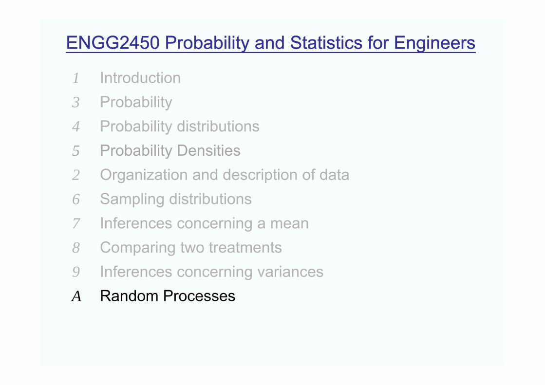
10.1 Why study Random Processes?

10 2 Definition of RP10.2 Definition of RP

10.3 Stationary RP & Ergodic RPy g

10.4 Autocorrelation Function of Ergodic RP

10.5 Power Spectral Density of Ergodic RP

10 6 N l RP (G i RP)10.6 Normal RP (Gaussian RP)

A random variable is defined by the following:

(revision) 4.1 Random variables (3)

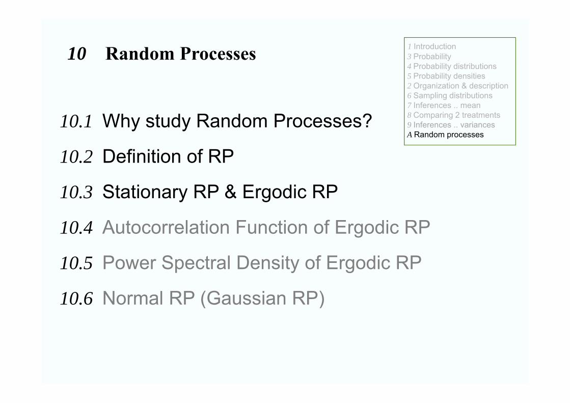
A random variable is defined by the following:

1. An experiment that can be repeated.The set that contains all possible outcomes of the experiment is called the sample space. A p p p psubset of the sample space is called an event.The outcome of an experiment is a number which is a sample of the random variable.

2 A function that associates a probability to each event2. A function that associates a probability to each event.

outcome sample spaceExperiment obtain a sample of the p p

{1 2 3 4 5 6}

p prandom variable

Throw a dice at trial i ande.g.1 xi {1,2,3,4,5,6}Throw a dice at trial i and

record the outcome xi.

gX

voltage x(t) (-10v, 10v)Measure the noise level of a phone line at time t and record the outcome x(t)

e.g.2X

the outcome x(t).

((revisionrevision)) Random Variable Random Variable (4)

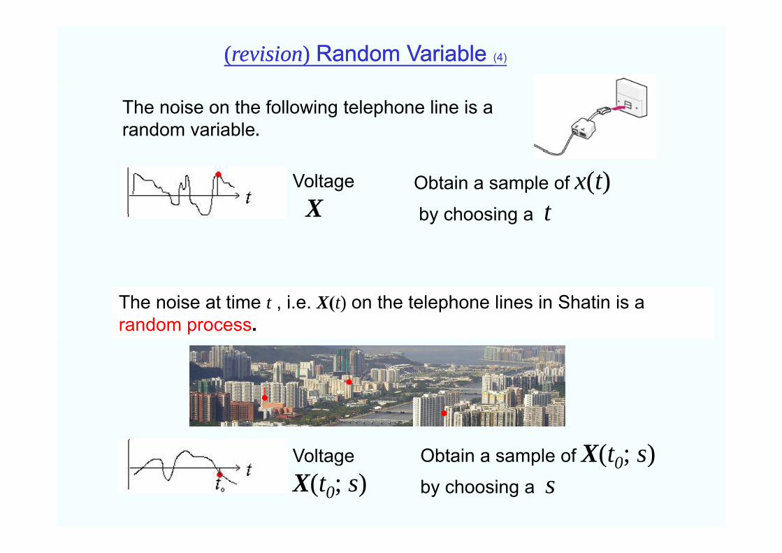
The noise on the following telephone line is a random variable.

VoltageX

Obtain a sample of x(t)by choosing a tX by choosing a t

The noise at time t0 , X(t0) on the telephone lines in Shatin is a random variable.

The noise at time t , i.e. X(t) on the telephone lines in Shatin is a random process.

Voltage Obtain a sample of X(t0; s)gX(t0; s)

p ( 0; )by choosing a s

10.1 Definition of Random ProcessesDefinition of Random Processes (5)

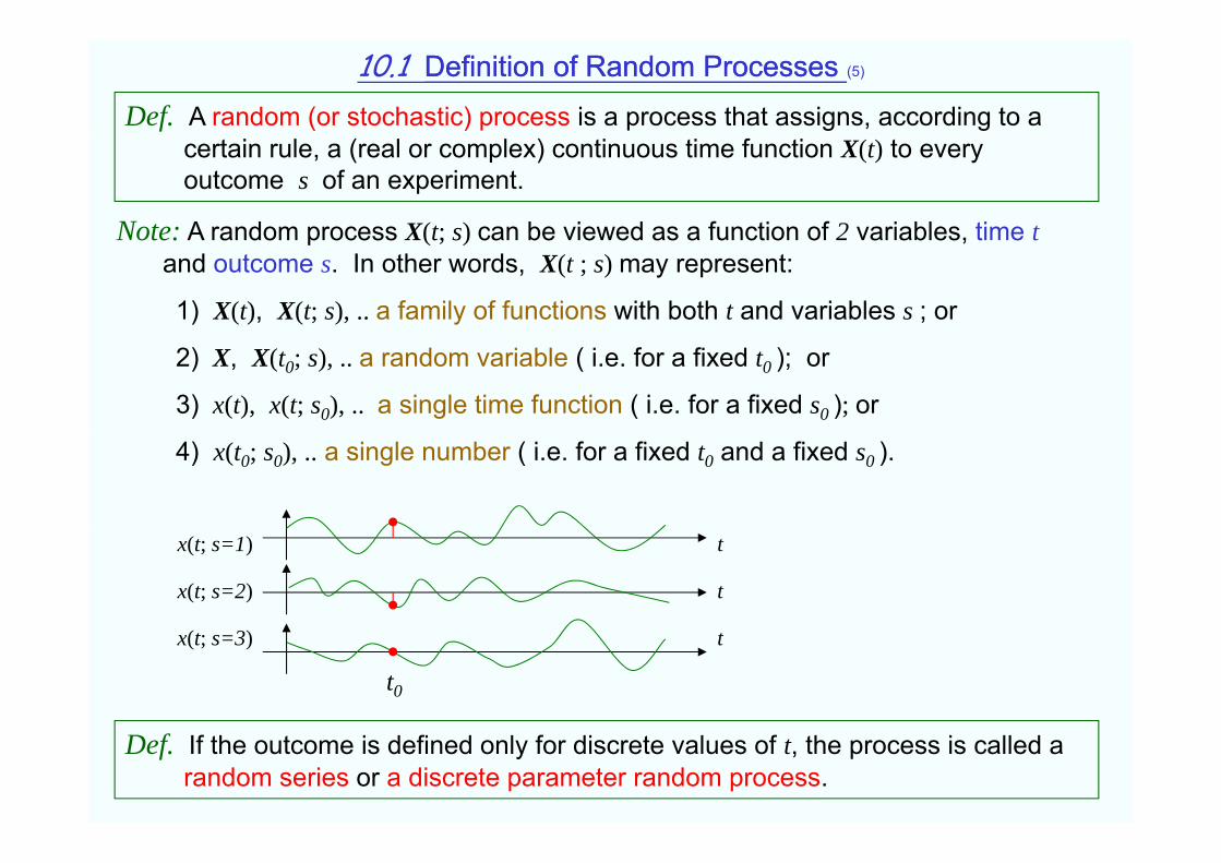
Def. A random (or stochastic) process is a process that assigns, according to a certain rule, a (real or complex) continuous time function X(t) to every outcome s of an experiment.

Note: A random process X(t; s) can be viewed as a function of 2 variables time tNote: A random process X(t; s) can be viewed as a function of 2 variables, time tand outcome s. In other words, X(t ; s) may represent:

1) X(t), X(t; s), .. a family of functions with both t and variables s ; or

2) X, X(t0; s), .. a random variable ( i.e. for a fixed t0 ); or

3) x(t), x(t; s0), .. a single time function ( i.e. for a fixed s0 ); or

4) x(t0; s0), .. a single number ( i.e. for a fixed t0 and a fixed s0 ).

x(t; s=1)

x(t; s=2)

t

t

x(t; s=3) t

t0

Def. If the outcome is defined only for discrete values of t, the process is called a random series or a discrete parameter random process.

Statistically Determined Random ProcessesStatistically Determined Random Processes (6)

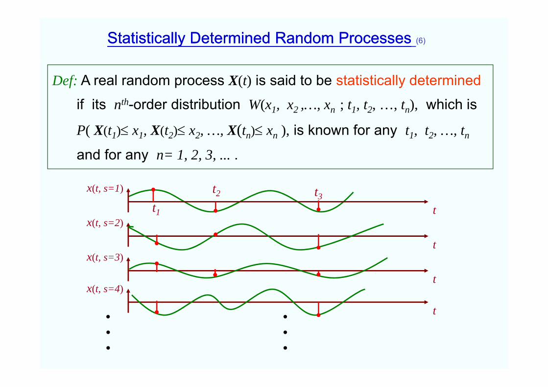
Def: A real random process X(t) is said to be statistically determined

if its nth-order distribution W(x x x ; t t t ) which isif its n -order distribution W(x1, x2 ,…, xn ; t1, t2, …, tn), which is

P( X(t1) x1, X(t2) x2, …, X(tn) xn ), is known for any t1, t2, …, tn

d fand for any n= 1, 2, 3, ... .

x(t, s=1) t2 t3( )

tt1

2

x(t, s=2)

t3

tx(t, s=3)

ttx(t, s=4)

t• •• •• •

Random ProcessesRandom Processes (7)

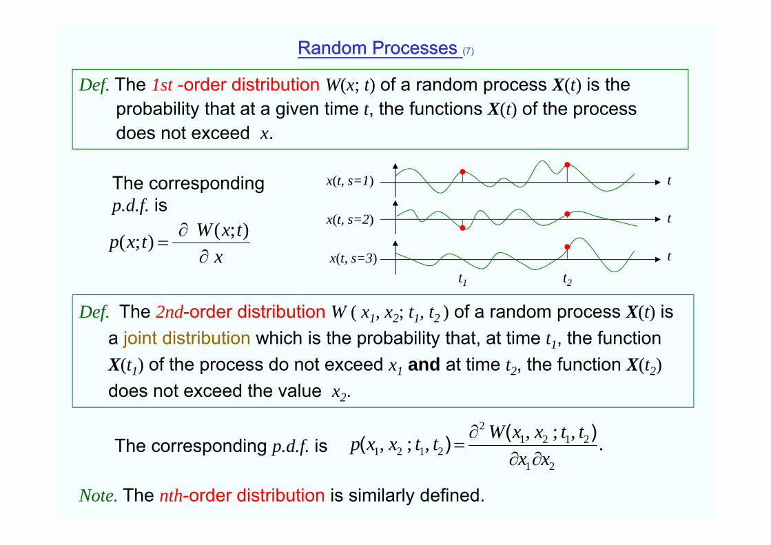
Def The 1st -order distribution W(x; t) of a random process X(t) is theDef. The 1st order distribution W(x; t) of a random process X(t) is the probability that at a given time t, the functions X(t) of the process does not exceed x.

x(t, s=1) tThe corresponding p.d.f. is

x(t, s=2)

x(t, s=3)

t

txtxWtxp

);();(

p.d.f. is

t1 t2

Def. The 2nd-order distribution W ( x1, x2; t1, t2 ) of a random process X(t) is a joint distrib tion hich is the probabilit that at time t the f nctiona joint distribution which is the probability that, at time t1, the function X(t1) of the process do not exceed x1 and at time t2, the function X(t2)does not exceed the value x2.does not exceed the value x2.

.,;,,;, 21212

2121 xxttxxWttxxp

)()(The corresponding p.d.f. is

Note. The nth-order distribution is similarly defined.

21 xx

The The 1st1st-- order Distribution order Distribution WW((xx;;tt)) (8)

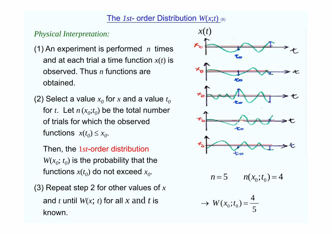
Physical Interpretation: x(t)y p

(1) An experiment is performed n times and at each trial a time function x(t) is ( )observed. Thus n functions are obtained.

(2) Select a value x0 for x and a value t0

for t. Let n (x0;t0) be the total number of trials for which the observed functions x(t0) x0.

Then, the 1st-order distributionW(x0;t0) is the probability that the functions (t ) do not exceedfunctions x(t0) do not exceed x0.

(3) Repeat step 2 for other values of xd

4);(5 00 txnn

4and t until W(x; t) for all x and t is known. 5

4);( 00 txW

The The 2nd2nd--Order Distribution Order Distribution WW((xx1, , xx2; ; tt1, , tt2)) (9)

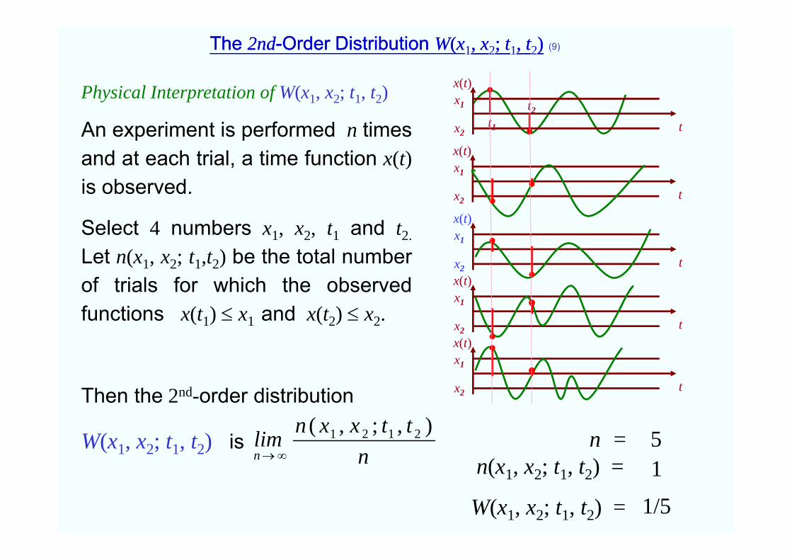
Ph i l I t t ti f W( t t ) x(t)Physical Interpretation of W(x1, x2; t1, t2)

An experiment is performed n timesd t h t i l ti f ti ( )

( )x1

x2 tt1

t2

x(t)and at each trial, a time function x(t)is observed.

x(t)x1

x2 t

(t)Select 4 numbers x1, x2, t1 and t2.

Let n(x1, x2; t1,t2) be the total numberf t i l f hi h th b d

x(t)x1

x2 tx(t)of trials for which the observed

functions x(t1) x1 and x(t2) x2.

x(t)x1

x2 tx(t)

Then the 2nd-order distribution

x(t)x1

x2 t

n = n(x1 x2; t1 t2) =

51n

ttxxnlimn

),;,( 2121

W(x1, x2; t1, t2) is

n(x1, x2; t1, t2)

W(x1, x2; t1, t2) = 1/5

1

Statistically Determined Random Processes Statistically Determined Random Processes (10)

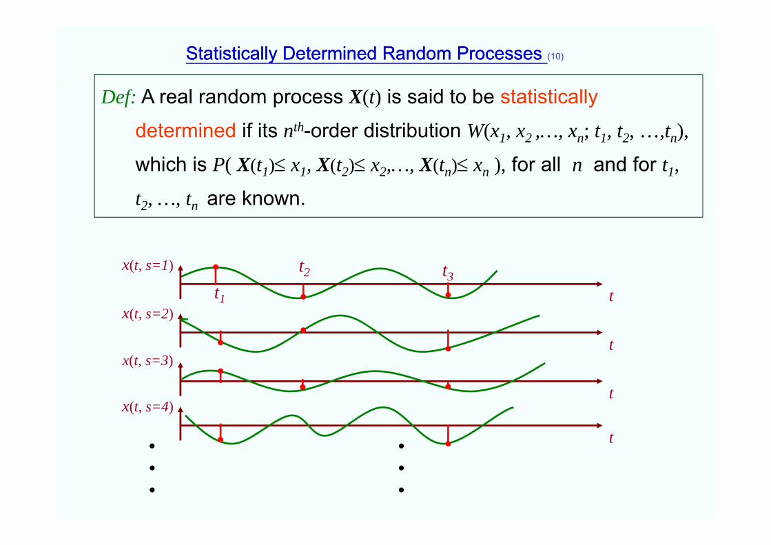
Def: A real random process X(t) is said to be statistically

determined if its nth-order distribution W(x1, x2 ,…, xn; t1, t2, …,tn),

which is P( X(t1) x1, X(t2) x2,…, X(tn) xn ), for all n and for t1,

t2, …, tn are known.

x(t, s=1) t2 t3( )

tt1

2

x(t, s=2)

t3

tx(t, s=3)

ttx(t, s=4)

t• •• •• •

Random Processes Random Processes (11)

Consider a random process X(t) of nth order joint p.d.f. p(x1, x2, …, xn; t1, t2, …, tn).

Note that:(1) n )((1)

n

nnn

nn xxttxxWttxxp

1

1111

...,,;...,,...,,;...,, )()(

(2) X(t1), X(t2), …, X(tn) are random variables obtained by sampling the random process X(t) at time t1, t2,…, tn. The x1, x2,…, xn inside p(x1, x2, …, xn; t1, t2, …, tn) and W(x1, x2, …, xn; t1, t2, …, tn) are not random variables but are values of the random variable X(t1), X(t2),…, X(tn) respectively.

10.2 Stationary RP & Ergodic RP (12)

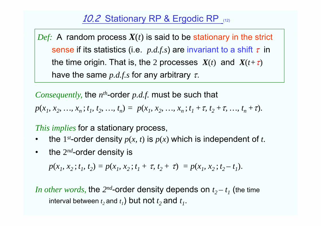
D f A random process X(t) is said to be stationary in the strictDef: A random process X(t) is said to be stationary in the strict sense if its statistics (i.e. p.d.f.s) are invariant to a shift in the time origin That is the 2 processes X(t) and X(t+)the time origin. That is, the 2 processes X(t) and X(t+)have the same p.d.f.s for any arbitrary .

Consequently, the nth-order p.d.f. must be such thatp(x1, x2, …, xn ; t1, t2, …, tn) = p(x1, x2, …, xn ; t1 +, t2 +, …, tn +).

This implies for a stationary process,• the 1st order density p(x t) is p(x) which is independent of t• the 1st-order density p(x, t) is p(x) which is independent of t.• the 2nd-order density is

( t t ) ( t + t + ) ( t t )p(x1, x2 ; t1, t2) = p(x1, x2 ; t1 + , t2 + ) = p(x1, x2 ; t2 – t1).

In other words the 2nd-order density depends on t t (the timeIn other words, the 2 -order density depends on t2 – t1 (the time interval between t2 and t1) but not t2 and t1.

The The 2nd2nd--Order Distribution Order Distribution WW((xx1, , xx2; ; tt1, , tt2)) (13)

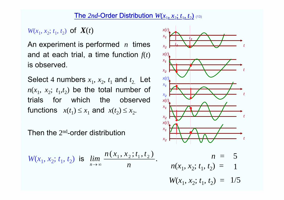
W(x1 x2; t1 t2) of X(t) x(t)W(x1, x2; t1, t2) of X(t)

An experiment is performed n timesand at each trial a time function f(t)

( )x1

x2 tt1

t2

x(t)and at each trial, a time function f(t)is observed.

S l t 4 b d L t

x(t)x1

x2 t

(t)Select 4 numbers x1, x2, t1 and t2. Letn(x1, x2; t1,t2) be the total number oftrials for which the observed

x(t)x1

x2 tx(t)trials for which the observed

functions x(t1) x1 and x(t2) x2.x(t)x1

x2 tx(t)

Then the 2nd-order distributionx(t)x1

x2 t

n = n(x1, x2; t1, t2) =

51

.),;,( 2121

nttxxnlim

n W(x1, x2; t1, t2) is

n(x1, x2; t1, t2)

W(x1, x2; t1, t2) = 1/5

1

The The 2nd2nd--Order Distribution Order Distribution WW((xx1, , xx2; ; tt1, , tt2)) (14)

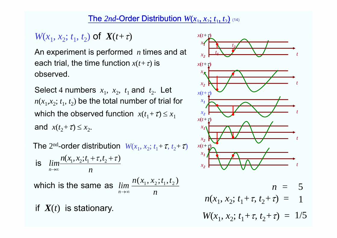
W(x1 x2; t1 t2) of X(t+) x(t+)W(x1, x2; t1, t2) of X(t+)An experiment is performed n times and at each trial, the time function x(t+) is

( )x1

x2 tt1

t2

x(t+)each trial, the time function x(t+) is observed.

Select 4 numbers x1, x2, t1 and t2. Let

x(t+)x1

x2 t

(t+ )Select 4 numbers x1, x2, t1 and t2. Letn(x1,x2; t1, t2) be the total number of trial for which the observed function x(t1+) x1

x(t+)x1

x2 tx(t+)

and x(t2+) x2. x(t+)

x1

x2 tx(t+)The 2nd order distribution W(x x ; t + t +) x(t+)

x1

x2 tn

ttxxnlimn

),;,( 2121

is

The 2nd-order distribution W(x1, x2; t1+, t2+)

nttxxnlim

n

),;,( 2121

as same the is which n =

n(x1 x2; t1+ t2+) =51n(x1, x2; t1+, t2+)

W(x1, x2; t1+, t2+) = 1/5

1if X(t) is stationary.

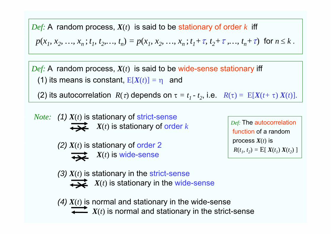
Def: A random process, X(t) is said to be stationary of order k iff

p(x1, x2, …, xn ; t1, t2,…, tn) = p(x1, x2, …, xn ; t1+, t2+ ,…, tn+) for n k .

stationary in the strict sense ... for any nDef: A random process, X(t) is said to be wide-sense stationary iff

(1) its means is constant, E[X(t)] = and

(1) X(t) is stationary of strict-sense

(2) its autocorrelation R() depends on = t1 - t2, i.e. R() = E[X(t+ ) X(t)].

Note: (1) X(t) is stationary of strict-senseX(t) is stationary of order k

(2) X(t) is stationar of order 2

Note:Def: The autocorrelation function of a random process X(t) is(2) X(t) is stationary of order 2

X(t) is wide-sense

p ( )R(t1, t2) = E[ X(t1) X(t2) ]

(3) X(t) is stationary in the strict-senseX(t) is stationary in the wide-sense

(4) X(t) is normal and stationary in the wide-senseX(t) is normal and stationary in the strict-sense

Given a random process X(t) of nth order joint p.d.f. p(x1, x2, …, xn; t1, t2, …, tn).

Random Processes Random Processes (16)

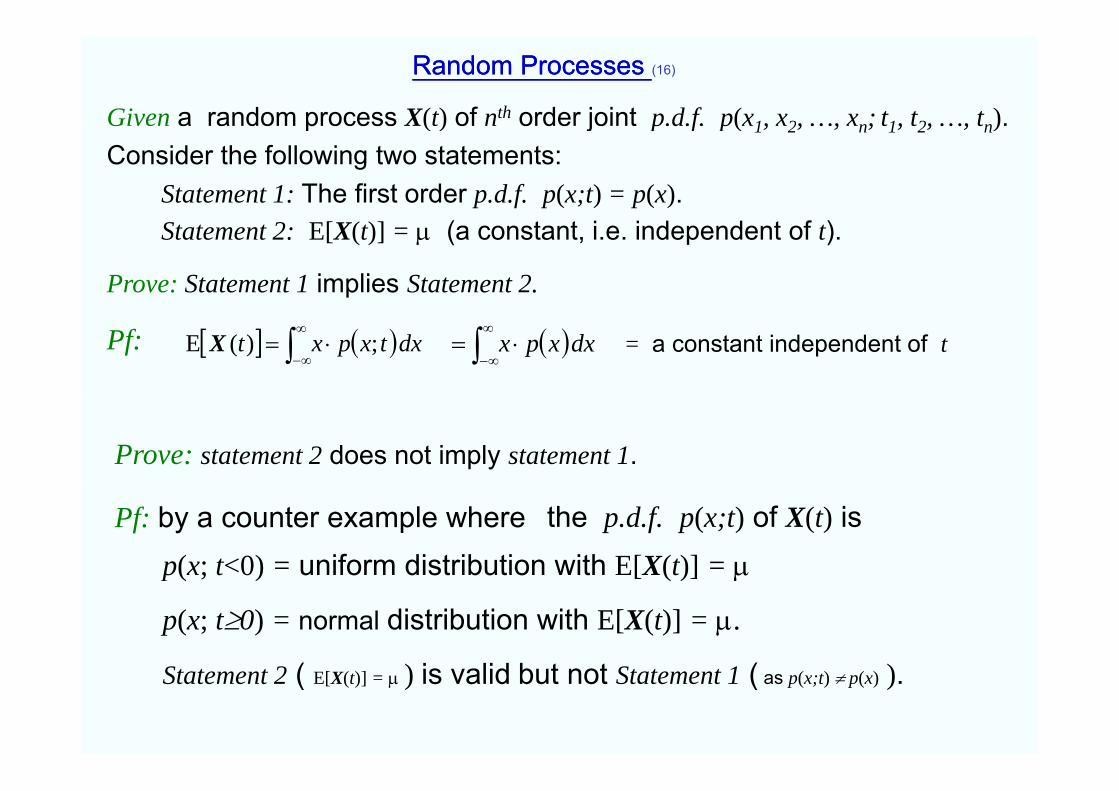
G p ( ) j p f p( 1, 2, , n; 1, 2, , n)Consider the following two statements:

Statement 1: The first order p.d.f. p(x;t) = p(x).Statement 2: E[X(t)] = (a constant, i.e. independent of t).

Prove: Statement 1 implies Statement 2.

Pf: dxtxpxt ;)(E

X dxxpx

= a constant independent of t

Prove: statement 2 does not imply statement 1.

Pf: by a counter example where p(x; t<0) = uniform distribution with E[X(t)] =

the p.d.f. p(x;t) of X(t) isp(x; t 0) u o d st but o t [ (t)]

p(x; t0) = normal distribution with E[X(t)] = .

( ) i lid b t t ( )Statement 2 ( E[X(t)] = ) is valid but not Statement 1 ( as p(x;t) p(x) ).

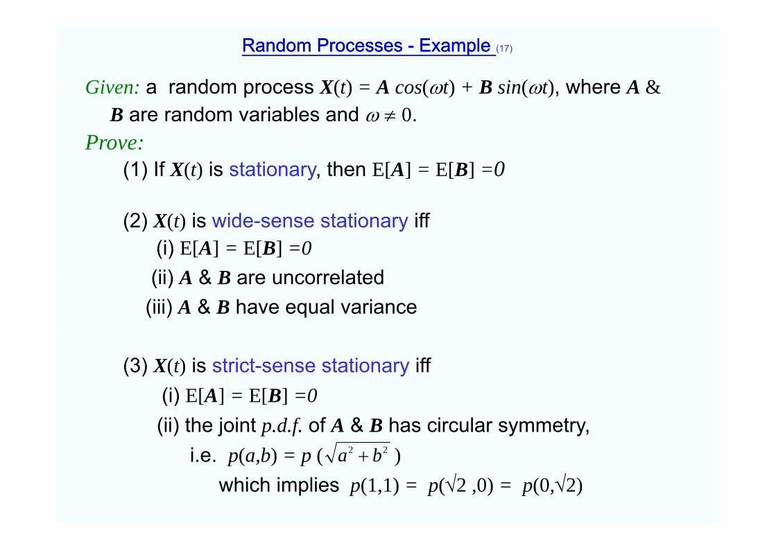
Given: a random process X(t) = A cos(t) + B sin(t) where A &

Random Processes Random Processes -- Example Example (17)

Given: a random process X(t) = A cos(t) + B sin(t), where A &B are random variables and 0.

Prove:ove(1) If X(t) is stationary, then E[A] = E[B] =0

(2) X(t) is wide-sense stationary iff (i) E[A] = E[B] =0(ii) A & B are uncorrelated(ii) A & B are uncorrelated(iii) A & B have equal variance

(3) X(t) is strict-sense stationary iff (i) E[A] = E[B] =0(i) E[A] E[B] 0(ii) the joint p.d.f. of A & B has circular symmetry,

i.e. p(a,b) = p ( )22 ba i.e. p(a,b) p ( )which implies p(1,1) = p(2 ,0) = p(0,2)

ba

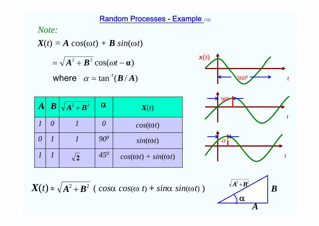
Note:Random Processes Random Processes -- Example Example (18)

X(t) = A cos(t) + B sin(t)

)cos(22 BA αtx(t)

)/(tan

)cos(

AB

BA1- where

αt

t3600

900

X(t)ba 22 BA A Bt

cos(t)0101

i ( t)900110

t

2 cos(t) + sin(t)45011

sin(t)900110

2

B22 BA X(t) = ( cos cos( t) + sin sin(t) )22 BA

B

A

X(t) ( cos cos( t) + sin sin(t) )BA

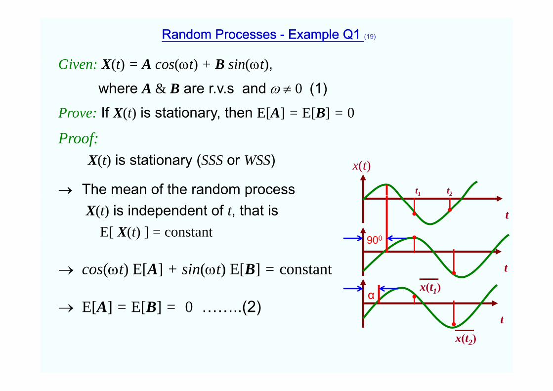
Gi X(t) A (t) + B i (t)

Random Processes Random Processes -- Example Q1 Example Q1 (19)

Given: X(t) = A cos(t) + B sin(t),

where A & B are r.v.s and 0 (1)

Prove: If X(t) is stationary, then E[A] = E[B] = 0

Proof:X(t) is stationary (SSS or WSS)

The mean of the random process

x(t)

t1 t2pX(t) is independent of t, that is

E[ X(t) ] = constantt

900

1 2

cos(t) E[A] + sin(t) E[B] = constant t

900

(t )

E[A] = E[B] = 0 ……..(2)t

αx(t1)

x(t2)

Given: X(t) = A cos(t) + B sin(t), where A & B are r.v.s and 0.

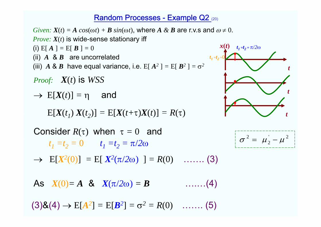
Random Processes Random Processes -- Example Q2 Example Q2 (20)

Prove: X(t) is wide-sense stationary iff (i) E[ A ] = E[ B ] = 0(ii) A & B are uncorrelated

x(t)t1 =t2 =0

t1 =t2 = /2

(iii) A & B have equal variance, i.e. E[ A2 ] = E[ B2 ] = 2

Proof: X(t) is WSSt

E[X(t)] = and

E[X(t ) X(t )] = E[X(t+)X(t)] = R()

t

tE[X(t1) X(t2)] E[X(t+)X(t)] R()

Consider R() when = 0 and

t

2'2 t1 =t2 = 0 t1 =t2 = /2

E[X2(0)] = E[ X2(/2) ] = R(0) ……. (3)

2

As X(0)= A & X(/2) = B ….…(4)

(3)&(4) E[A2] = E[B2] = 2 = R(0) ……. (5)

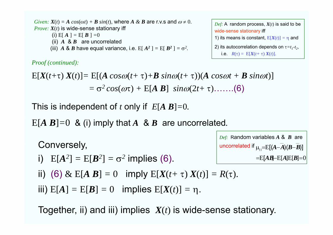
Given: X(t) = A cos(t) + B sin(t), where A & B are r.v.s and 0.Prove: X(t) is wide-sense stationary iff

(i) E[ A ] = E[ B ] =0

Def: A random process, X(t) is said to be wide-sense stationary iff1) its means is constant E[X(t)] = and( ) [ ] [ ]

(ii) A & B are uncorrelated(iii) A & B have equal variance, i.e. E[ A2 ] = E[ B2 ] = 2.

1) its means is constant, E[X(t)] = and

2) its autocorrelation depends on =t1-t2, i.e. R() = E[X(t+ ) X(t)].

Proof (continued):Proof (continued):

E[X(t+) X(t)]= E[(A cos(t+ )+B sin(t+ ))(A cost + B sint)]= 2 cos() + E[A B] sin(2t+ )…….(6)

This is independent of t only if E[A B]=0.

cos() E[A B] sin(2t )…….(6)

ConverselyDef: Random variables A & B are

l t d if

E[A B]=0 & (i) imply that A & B are uncorrelated.

Conversely, i) E[A2] = E[B2] = 2 implies (6).ii) (6) & E[A B] 0 i l E[X( ) X( )] R( )

uncorrelated if

0][][]11

BAAB

BBAA

[

)]()[(

EEE

E

ii) (6) & E[A B] = 0 imply E[X(t+ ) X(t)] = R().iii) E[A] = E[B] = 0 implies E[X(t)] = .

Together, ii) and iii) implies X(t) is wide-sense stationary.

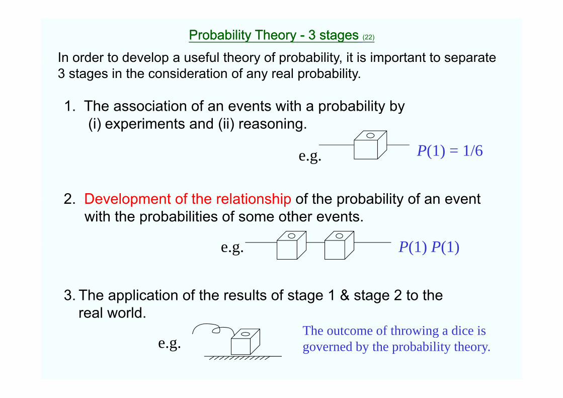
Probability Theory Probability Theory -- 3 stages3 stages (22)

In order to develop a useful theory of probability, it is important to separate p y p y, p p3 stages in the consideration of any real probability.

1 The association of an events with a probability by1. The association of an events with a probability by (i)experiments and (ii) reasoning.

e g P(1) = 1/6e.g. P(1) 1/6

2 Development of the relationship of the probability of an event

P(1) P(1)

2. Development of the relationship of the probability of an event with the probabilities of some other events.

e.g. P(1) P(1)

f f &3. The application of the results of stage 1 & stage 2 to the real world.

The outcome of throwing a dice ise.g.

The outcome of throwing a dice is governed by the probability theory.

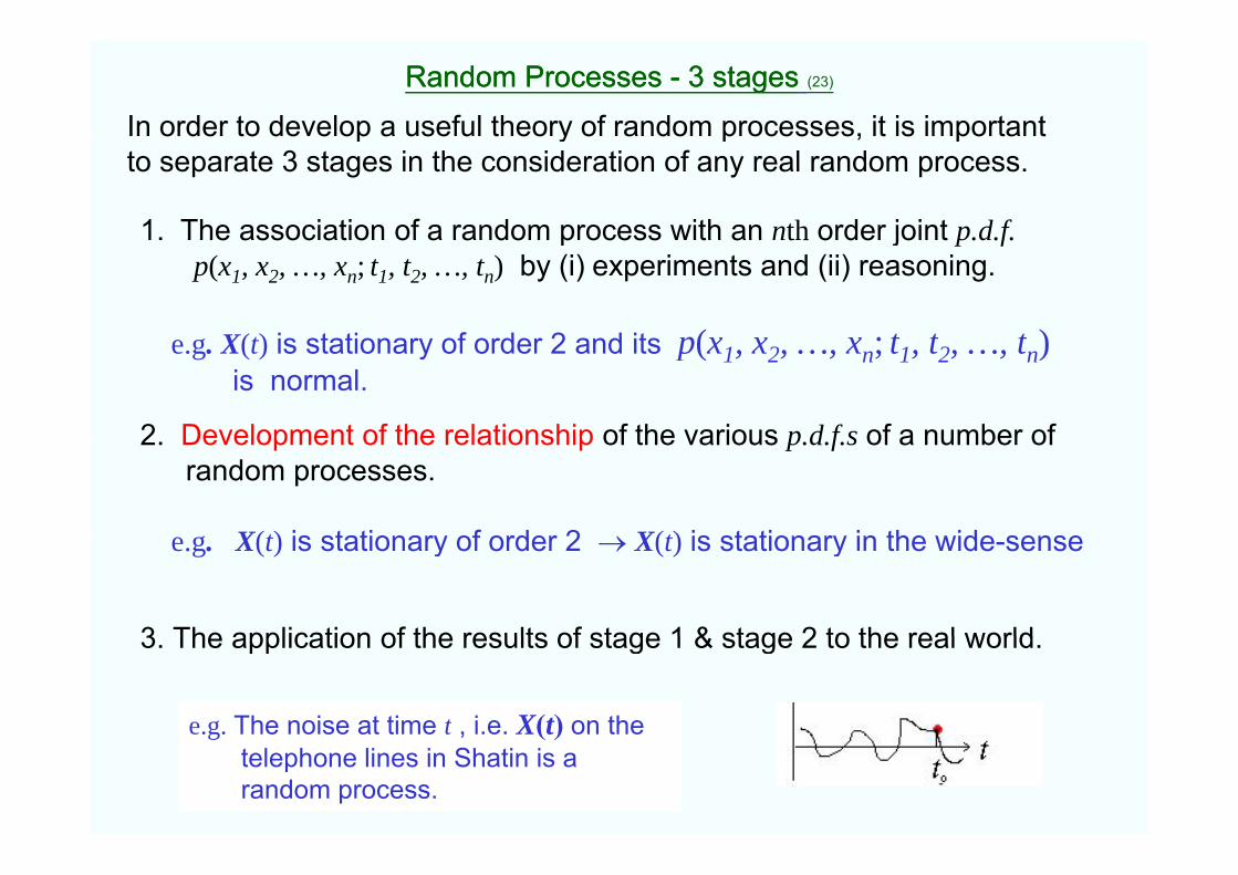
Random Processes Random Processes -- 3 stages3 stages (23)

In order to develop a useful theory of random processes, it is important p y p , pto separate 3 stages in the consideration of any real random process.

1. The association of a random process with an nth order joint p.d.f.1. The association of a random process with an nth order joint p.d.f.p(x1, x2, …, xn; t1, t2, …, tn) by (i)experiments and (ii) reasoning.

X(t) is stationary of order 2 and its p(x x x ; t t t )

2 Development of the relationship of the various p d f s of a number of

e.g. X(t) is stationary of order 2 and its p(x1, x2, …, xn; t1, t2, …, tn)is normal.

2. Development of the relationship of the various p.d.f.s of a number of random processes.

X(t) is stationary of order 2 X(t) is stationary in the wide sense

3 The application of the results of stage 1 & stage 2 to the real world

e.g. X(t) is stationary of order 2 X(t) is stationary in the wide-sense

3. The application of the results of stage 1 & stage 2 to the real world.

e.g. The noise at time t , i.e. X(t) on the g , ( )telephone lines in Shatin is a random process.

Stationary Random Process Stationary Random Process (24)

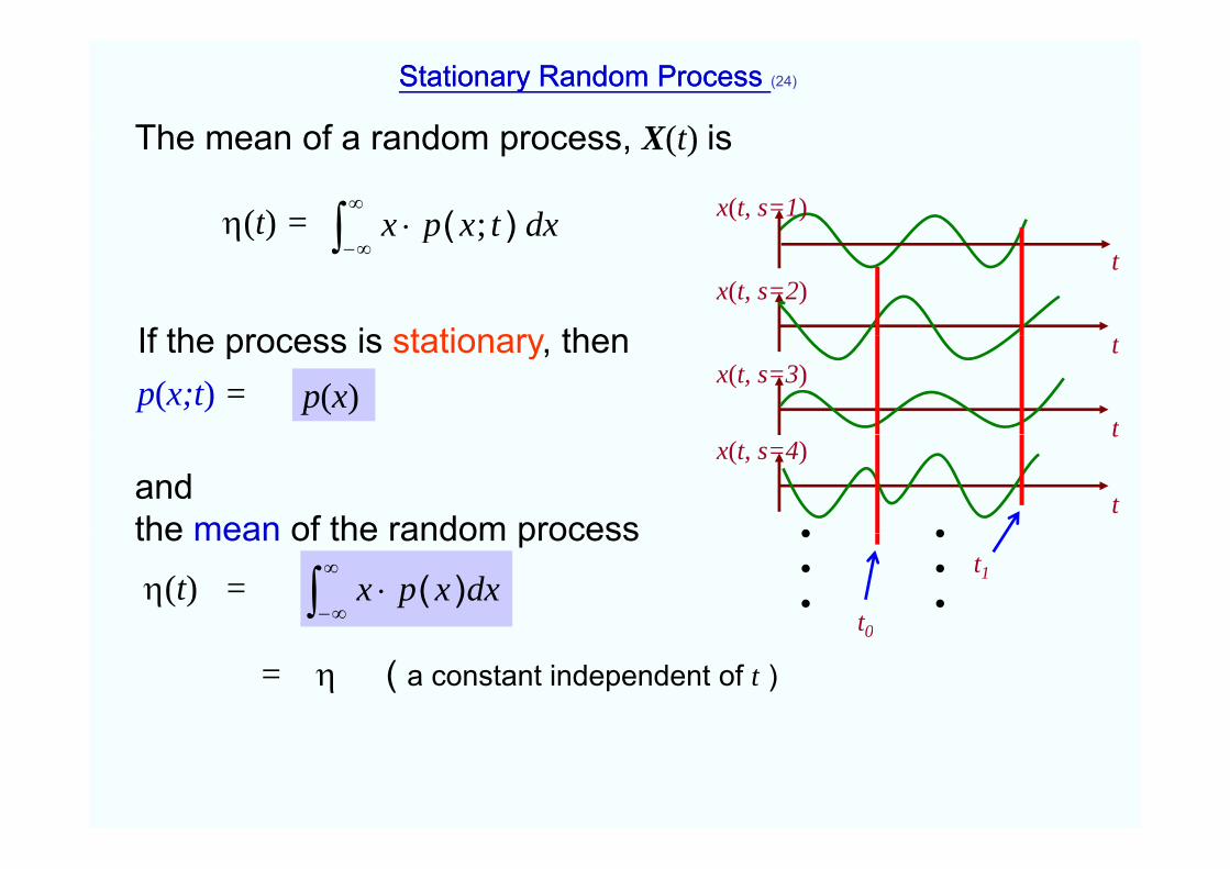
The mean of a random process X(t) isThe mean of a random process, X(t) is

(t) =

dxtxpx )( ; x(t, s=1)

If the process is stationary then

( ) p )( ;

tx(t, s=2)

If the process is stationary, thenp(x;t) =

tx(t, s=3)

tp(x)

• •

tx(t, s=4)

tand the mean of the random process • •

• •• •

t1

t0

dxxpx )(

the mean of the random process

(t) =0

= ( a constant independent of t )

Ergodicity Ergodicity (25)

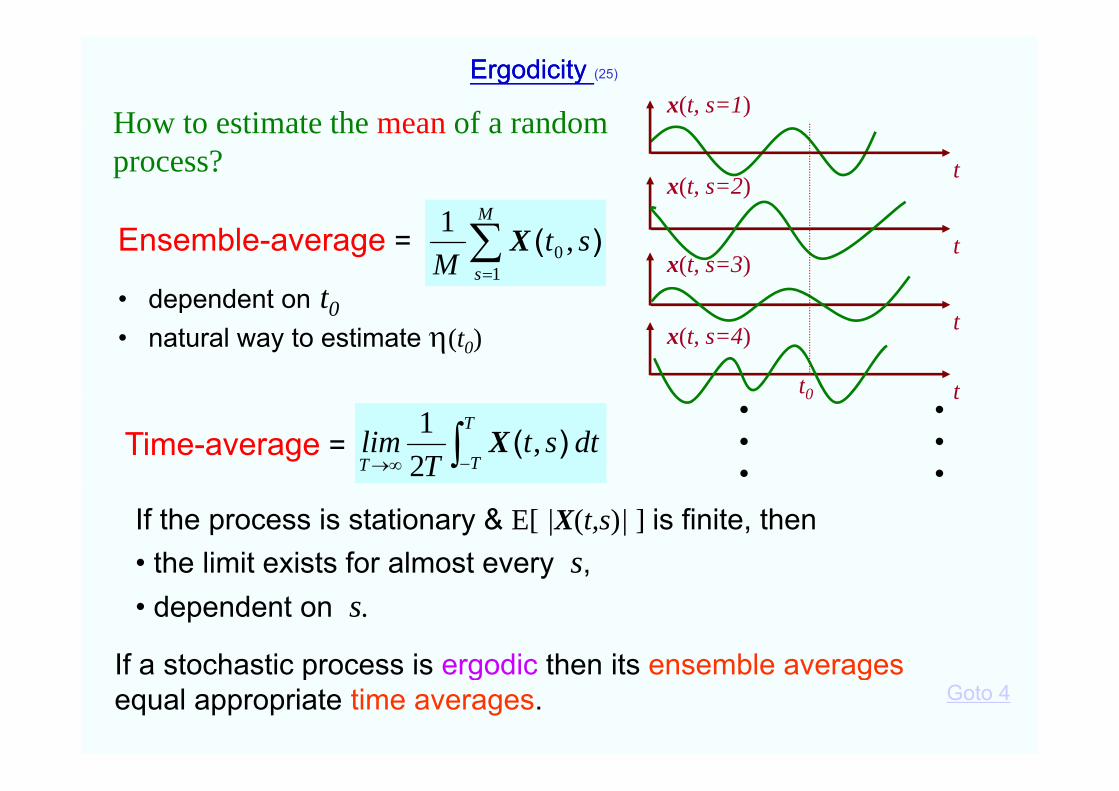
How to estimate the mean of a random x(t, s=1)How to estimate the mean of a random process?

M1

tx(t, s=2)

Ensemble-average =

• dependent on t0

M

sst

M 10 ,1 )(X t

x(t, s=3)dependent on t0

• natural way to estimate (t0)tx(t, s=4)

tt0

T

TTdtst

Tlim )( ,

21 X

• •• •• •

t0

Time-average =

If the process is stationary & E[ |X(t,s)| ] is finite, then• the limit exists for almost every s,

If a stochastic process is ergodic then its ensemble averages

y ,• dependent on s.

If a stochastic process is ergodic then its ensemble averagesequal appropriate time averages. Goto 4

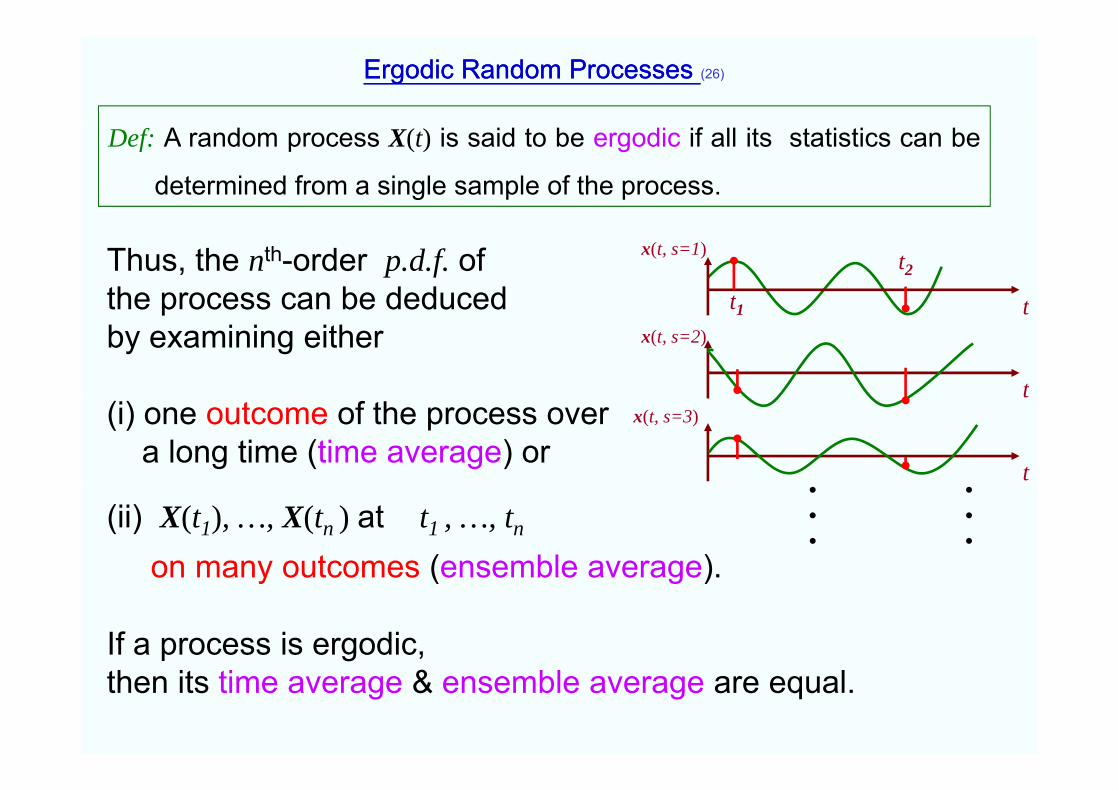
Ergodic Random Processes Ergodic Random Processes (26)

Def: A random process X(t) is said to be ergodic if all its statistics can be

determined from a single sample of the process.

Thus, the nth-order p.d.f. ofthe process can be deduced tt1

t2x(t, s=1)

the process can be deducedby examining either

tt1

t

x(t, s=2)

(i) one outcome of the process overa long time (time average) or

t

t

x(t, s=3)

(ii) X(t1), …, X(tn ) at t1 , …, tn

on many outcomes (ensemble average).

• •• •• •

on many outcomes (ensemble average).

If a process is ergodic, then its time average & ensemble average are equal.