Embed Size (px)
Citation preview
Engineering Optics Engineering Optics
Understanding light?• Reflection and refraction• Geometric optics ( << D): ray tracing, matrix methods
• Physical optics ( ~ D): wave equation, diffraction, interference • Polarization • Interaction with resonance transitions
Optical devices?• Lenses • Mirrors• Polarizing optics
• Microscopes and telescopes• Lasers• Fiber optics• ……………and many more
Engineering OpticsEngineering Optics
In mechanical engineering, a primary motivation for studying optics is to learn how to use optical techniques for making measurements. Optical techniques are widely used in many areas of the thermal sciences for measuring system temperatures, velocities, and species on a time- and space-resolved basis. In many cases these non-intrusive optical devices have significant advantages over physical probes that perturb the system that is being studied.
Lasers are finding increasing use as machining and manufacturing devices. All types of lasers from continuous-wave lasers to lasers with femtosecond pulse lengths are being used to cut and process
materials.
Huygen’s Wavelet Concept Huygen’s Wavelet Concept
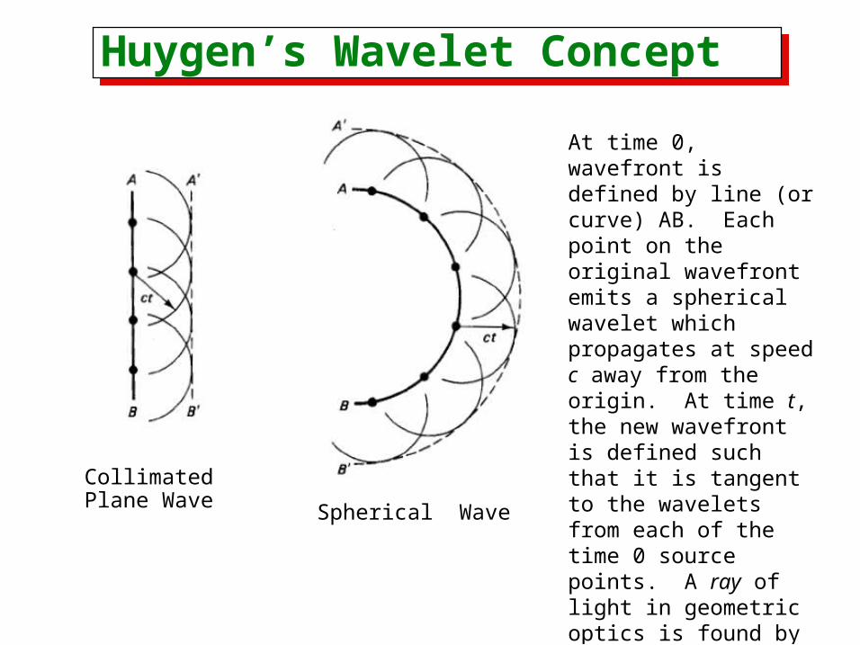
Collimated Plane Wave
Spherical Wave
At time 0, wavefront is defined by line (or curve) AB. Each point on the original wavefront emits a spherical wavelet which propagates at speed c away from the origin. At time t, the new wavefront is defined such that it is tangent to the wavelets from each of the time 0 source points. A ray of light in geometric optics is found by drawing a line from the source point to the tangent point for each wavelet.
Geometric Optics: The Refractive Index
Geometric Optics: The Refractive Index
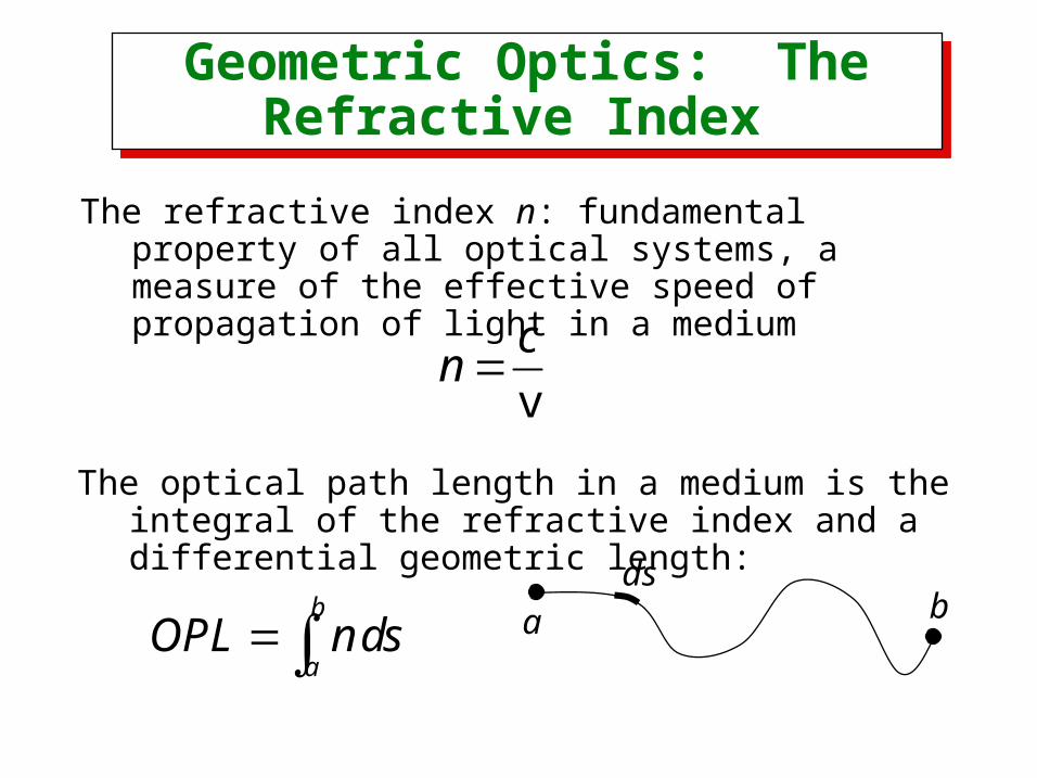
The refractive index n: fundamental property of all optical systems, a measure of the effective speed of propagation of light in a medium
v
cn
The optical path length in a medium is the integral of the refractive index and a differential geometric length:
b
aOPL n ds a b
ds
Fermat’s Principle: Law of Reflection Fermat’s Principle: Law of Reflection
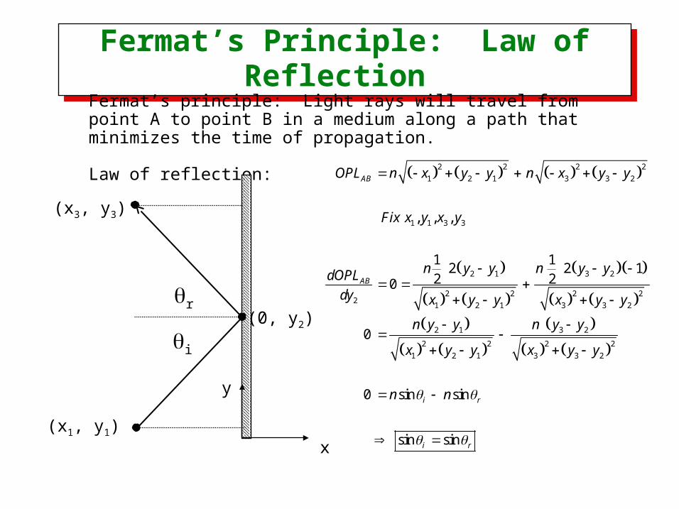
Fermat’s principle: Light rays will travel from point A to point B in a medium along a path that minimizes the time of propagation.
Law of reflection:
x
y
(x1, y1)
(0, y2)
(x3, y3)
r
i
2 2 2 2
1 2 1 3 3 2
1 1 3 3
2 1 3 2
2 2 2 22
1 2 1 3 3 2
2 1 3 2
2 2 2 2
1 2 1 3 3 2
, , ,
1 12 2 1
2 20
0
0 sin sin
sin sin
AB
AB
i r
i r
OPL n x y y n x y y
Fix x y x y
n y y n y ydOPL
dy x y y x y y
n y y n y y
x y y x y y
n n
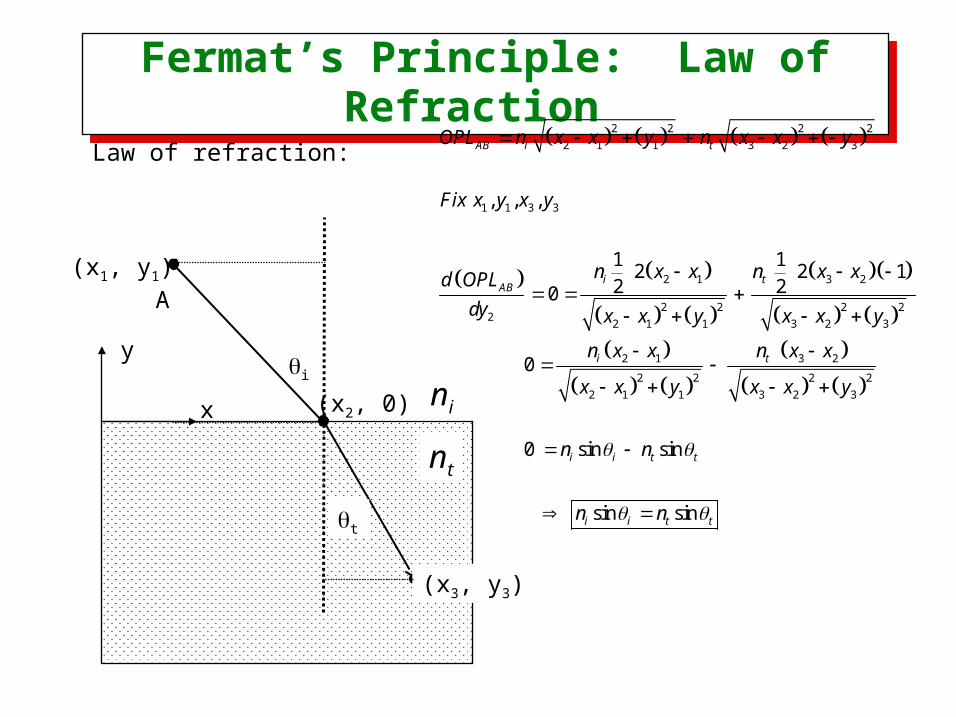
Fermat’s Principle: Law of Refraction Fermat’s Principle: Law of Refraction
Law of refraction:
x
y
(x1, y1)
(x2, 0)
(x3, y3)
t
i
2 2 2 2
2 1 1 3 2 3
1 1 3 3
2 1 3 2
2 2 2 22
2 1 1 3 2 3
2 1 3 2
2 2 2 2
2 1 1 3 2 3
, , ,
1 12 2 1
2 20
0
0 sin sin
sin sin
AB i t
i tAB
i t
i i t t
i i t t
OPL n x x y n x x y
Fix x y x y
n x x n x xd OPL
dy x x y x x y
n x x n x x
x x y x x y
n n
n n
A
ni
nt
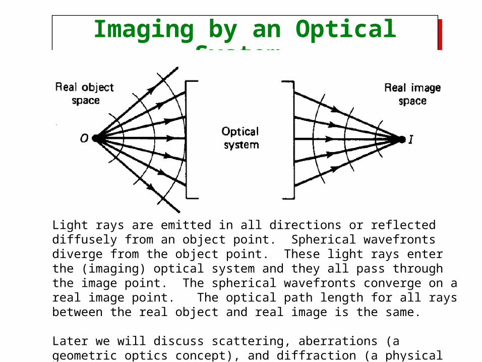
Imaging by an Optical System Imaging by an Optical System
Light rays are emitted in all directions or reflected diffusely from an object point. Spherical wavefronts diverge from the object point. These light rays enter the (imaging) optical system and they all pass through the image point. The spherical wavefronts converge on a real image point. The optical path length for all rays between the real object and real image is the same.
Later we will discuss scattering, aberrations (a geometric optics concept), and diffraction (a physical optics concept) which cause image degradation.
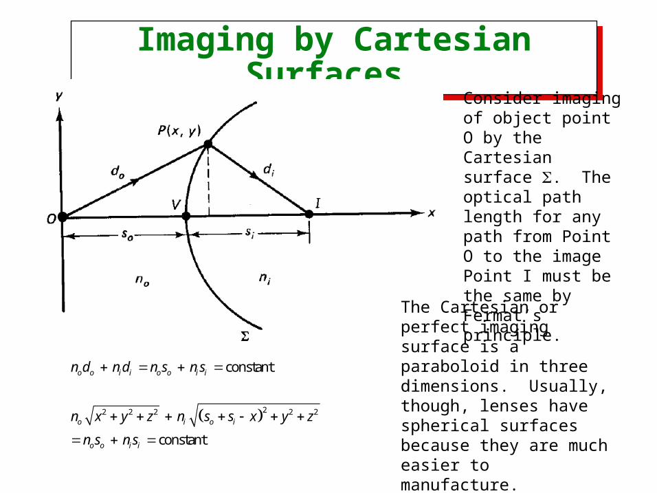
Imaging by Cartesian Surfaces Imaging by Cartesian Surfaces
Consider imaging of object point O by the Cartesian surface . The optical path length for any path from Point O to the image Point I must be the same by Fermat’s principle.
22 2 2 2 2
constant
constant
o o i i o o i i
o i o i
o o i i
n d n d n s n s
n x y z n s s x y z
n s n s
The Cartesian or perfect imaging surface is a paraboloid in three dimensions. Usually, though, lenses have spherical surfaces because they are much easier to manufacture.
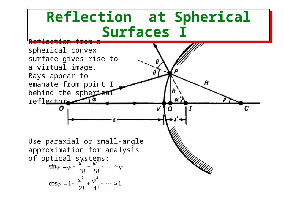
Reflection at Spherical Surfaces I Reflection at Spherical Surfaces I
Use paraxial or small-angle approximation for analysis of optical systems: 3 5
2 4
sin3! 5!
cos 1 12! 4!
Reflection from a spherical convex surface gives rise to a virtual image. Rays appear to emanate from point I behind the spherical reflector.
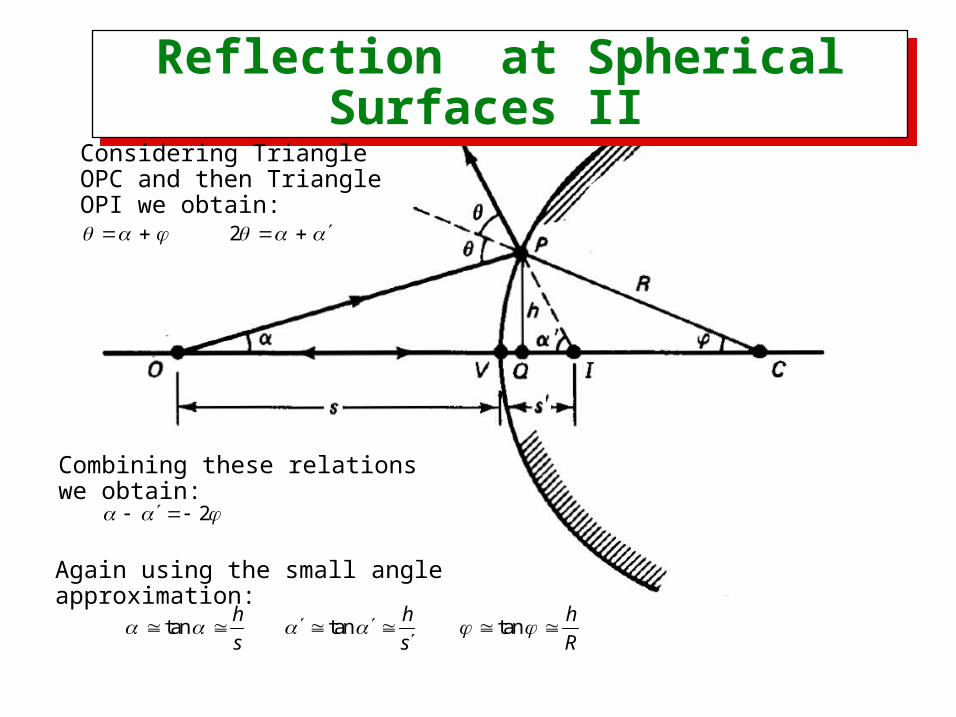
Reflection at Spherical Surfaces II Reflection at Spherical Surfaces II
Considering Triangle OPC and then Triangle OPI we obtain:
2
Combining these relations we obtain:
2
Again using the small angle approximation:
tan tan tanh h h
s s R
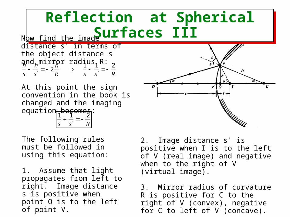
Reflection at Spherical Surfaces III Reflection at Spherical Surfaces III Now find the image distance s' in terms of the object distance s and mirror radius R:
1 1 22
h h h
s s R s s R
At this point the sign convention in the book is changed and the imaging equation becomes:
1 1 2
s s R
The following rules must be followed in using this equation:
1. Assume that light propagates from left to right. Image distance s is positive when point O is to the left of point V.
2. Image distance s' is positive when I is to the left of V (real image) and negative when to the right of V (virtual image).
3. Mirror radius of curvature R is positive for C to the right of V (convex), negative for C to left of V (concave).
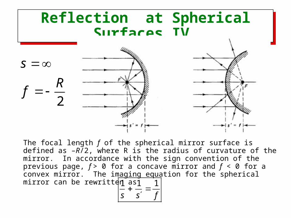
Reflection at Spherical Surfaces IV Reflection at Spherical Surfaces IV
The focal length f of the spherical mirror surface is defined as –R/2, where R is the radius of curvature of the mirror. In accordance with the sign convention of the previous page, f > 0 for a concave mirror and f < 0 for a convex mirror. The imaging equation for the spherical mirror can be rewritten as
1 1 1
s s f
2
s
Rf
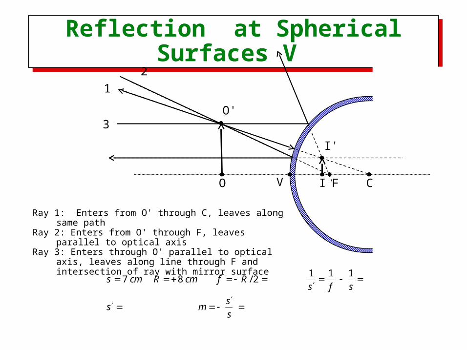
Reflection at Spherical Surfaces V Reflection at Spherical Surfaces V
CFO I
1
2
3
I'
O'
Ray 1: Enters from O' through C, leaves along same path Ray 2: Enters from O' through F, leaves parallel to optical axis Ray 3: Enters through O' parallel to optical axis, leaves along
line through F and intersection of ray with mirror surface
1 1 17 8 / 2s cm R cm f R
s f s
ss m
s
V
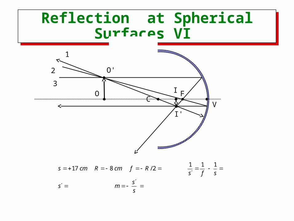
Reflection at Spherical Surfaces VI Reflection at Spherical Surfaces VI
CFO I
1
2
3
I'
O'
1 1 117 8 / 2s cm R cm f R
s f s
ss m
s
V
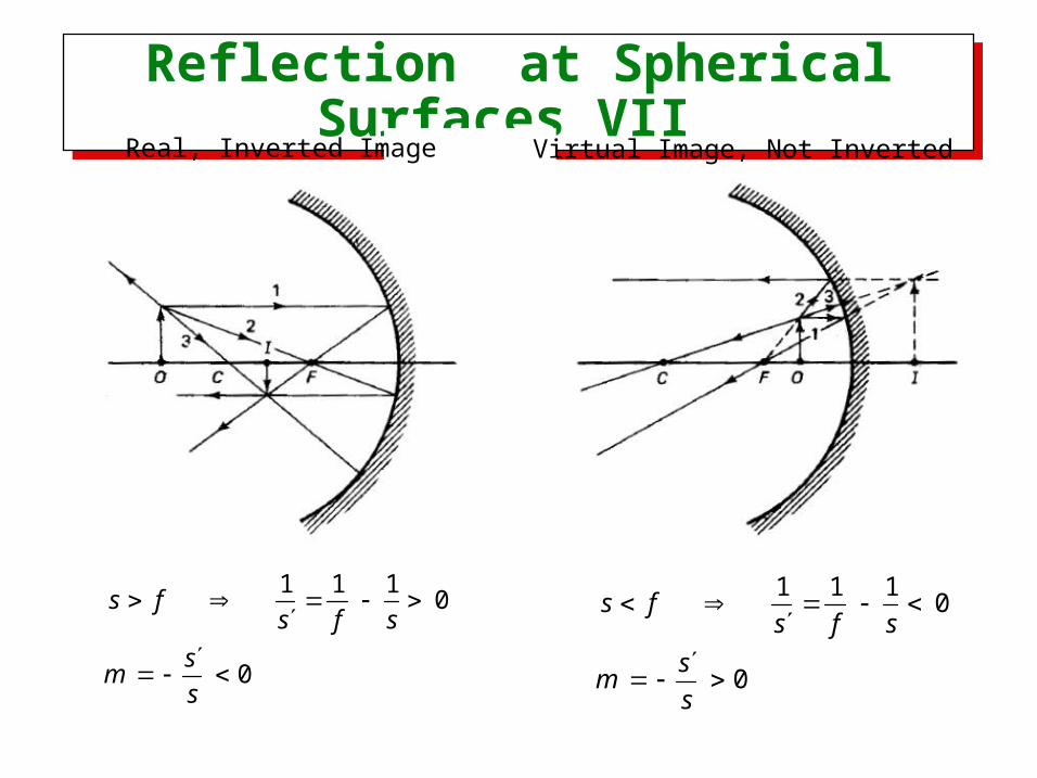
Reflection at Spherical Surfaces VII Reflection at Spherical Surfaces VII
1 1 10
0
s fs f s
sm
s
1 1 10
0
s fs f s
sm
s
Real, Inverted Image Virtual Image, Not Inverted
Geometrical Optics Geometrical Optics
Index of refraction for transparent optical materials• Refraction by spherical surfaces• The thin lens approximation• Imaging by thin lenses• Magnification factors for thin lenses• Two-lens systems
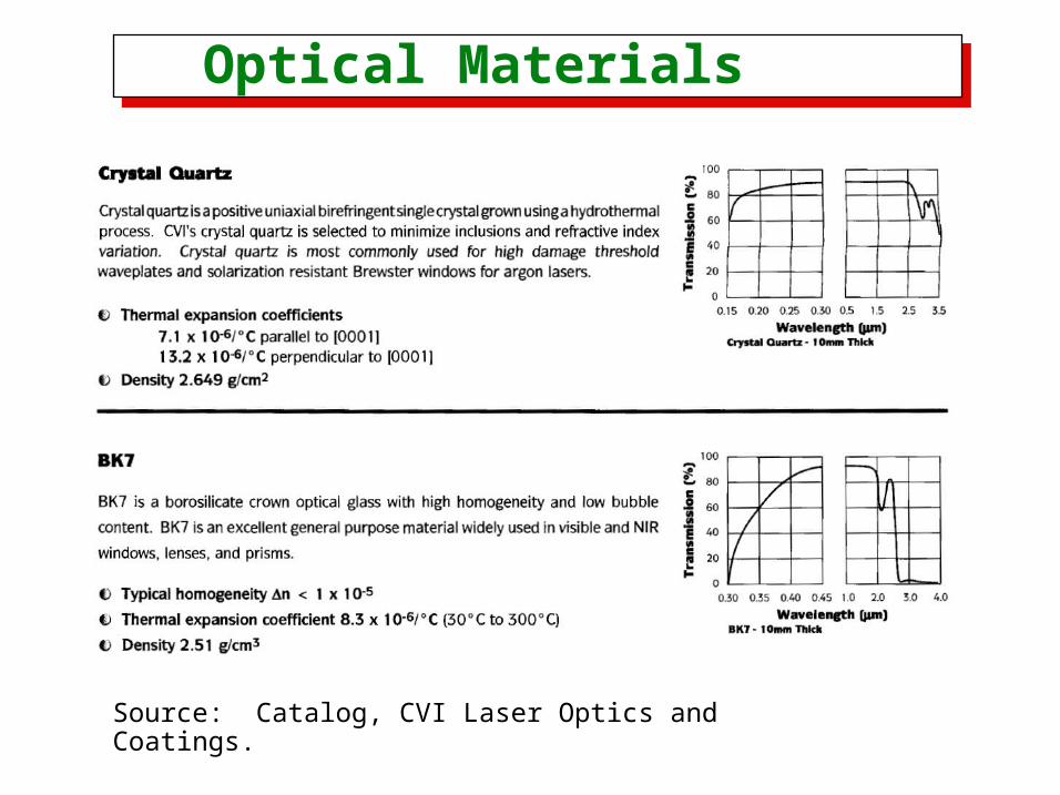
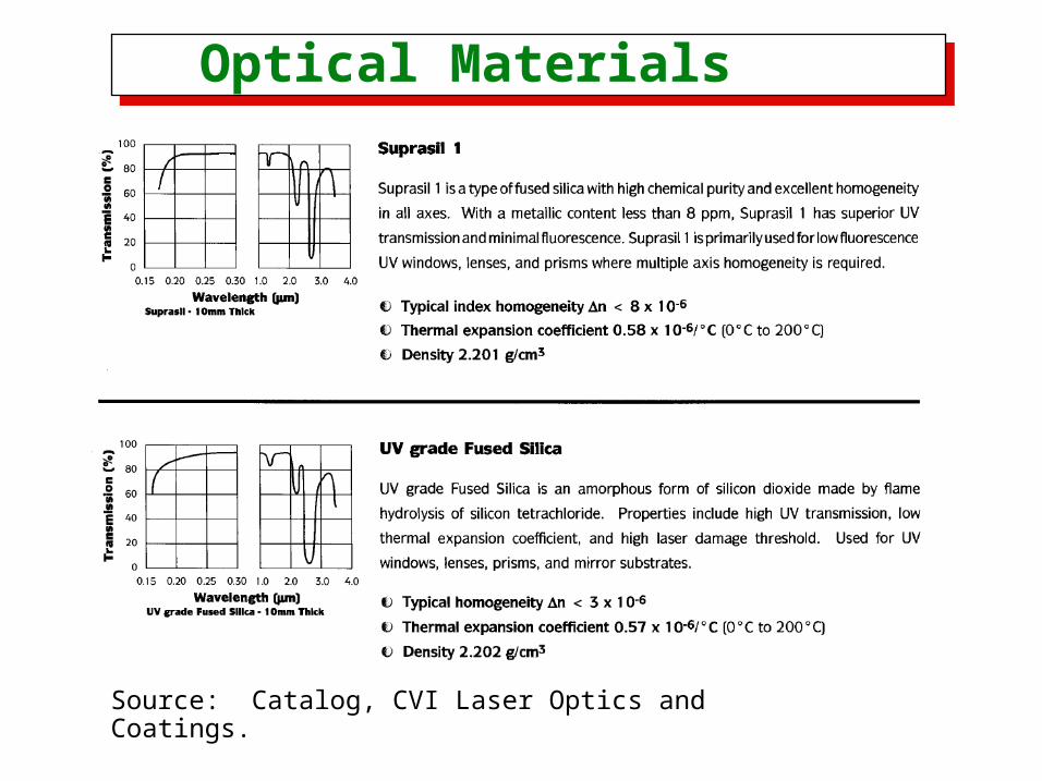
Optical Materials Optical Materials
Source: Catalog, CVI Laser Optics and Coatings.
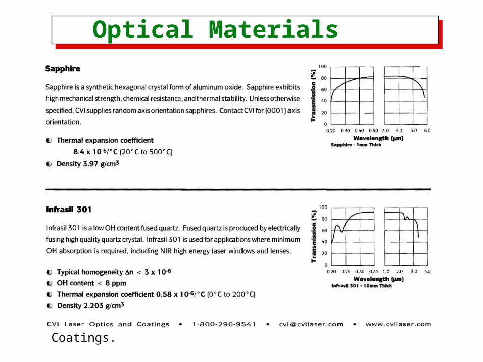
Optical Materials Optical Materials
Source: Catalog, CVI Laser Optics and Coatings.
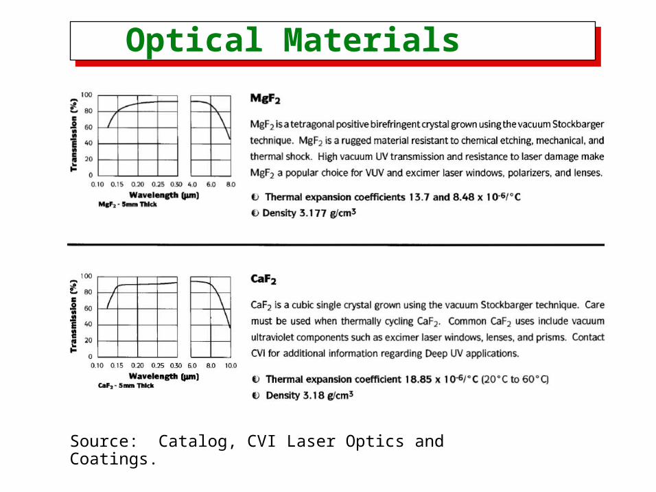
Optical Materials Optical Materials
Source: Catalog, CVI Laser Optics and Coatings.
Optical Materials Optical Materials
Source: Catalog, CVI Laser Optics and Coatings.
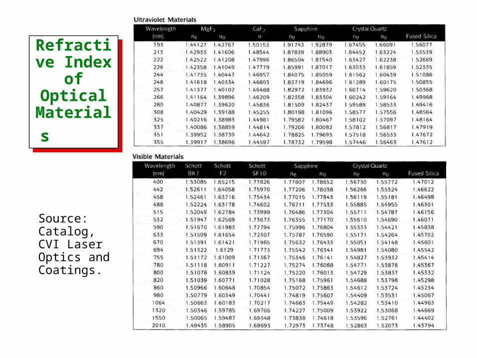
Refractive Index of Optical
Materials
Refractive Index of Optical
Materials
Source:Catalog, CVI Laser Optics and Coatings.
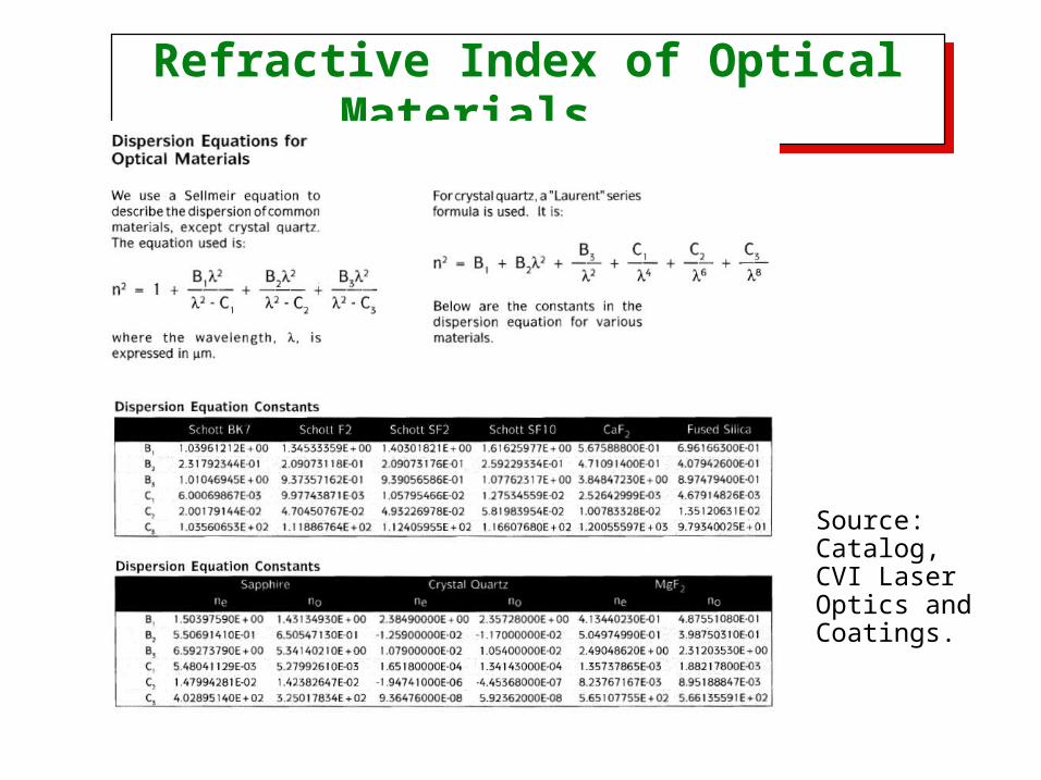
Refractive Index of Optical Materials
Refractive Index of Optical Materials
Source:Catalog, CVI Laser Optics and Coatings.
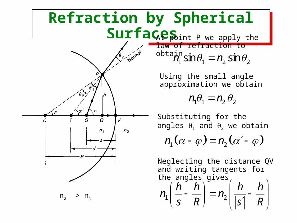
Refraction by Spherical Surfaces
Refraction by Spherical Surfaces
n2 > n1
At point P we apply the law of refraction to obtain
1 1 2 2sin sinn n
Using the small angle approximation we obtain
1 1 2 2n n
Substituting for the angles 1 and 2 we obtain
1 2n n
Neglecting the distance QV and writing tangents for the angles gives
1 2
h h h hn n
s R s R
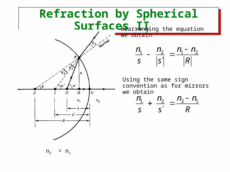
Refraction by Spherical Surfaces II Refraction by Spherical Surfaces II
n2 > n1
Rearranging the equation we obtain
Using the same sign convention as for mirrors we obtain
1 2 1 2n n n n
s s R
1 2 2 1n n n n
s s R
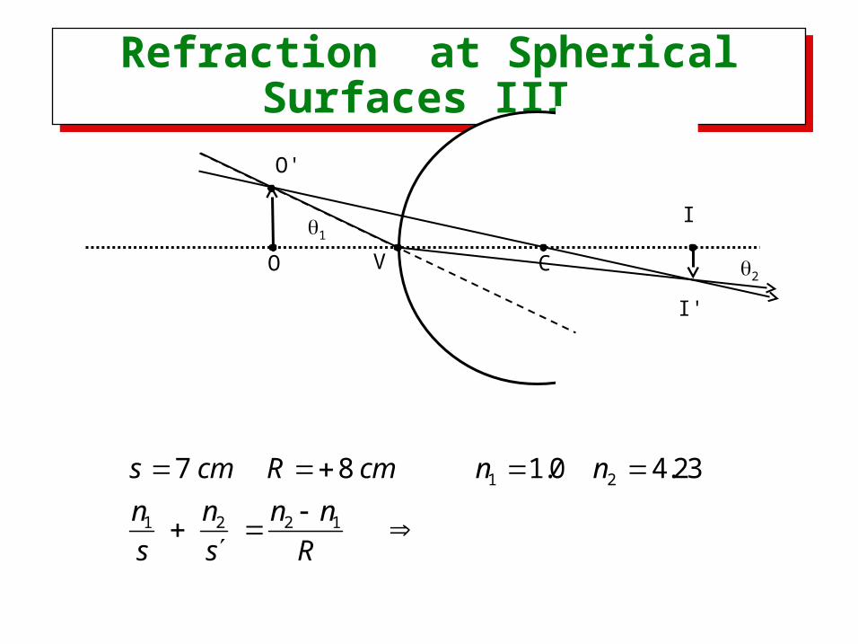
Refraction at Spherical Surfaces III Refraction at Spherical Surfaces III
CO
I
I'
O'
1 2
1 2 2 1
7 8 1.0 4.23s cm R cm n n
n n n n
s s R
V
1
2
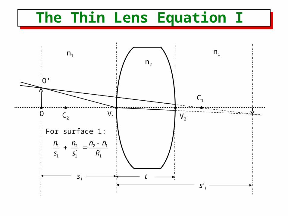
The Thin Lens Equation I The Thin Lens Equation I
O
O'
t
C2
C1
n1n1
n2
s1
s'1
1 2 2 1
1 1 1
n n n n
s s R
V1 V2
For surface 1:
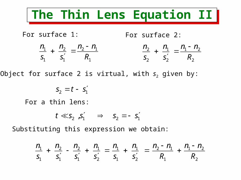
The Thin Lens Equation II The Thin Lens Equation II
1 2 2 1
1 1 1
n n n n
s s R
For surface 1:
2 1 1 2
2 2 2
n n n n
s s R
For surface 2:
2 1s t s
Object for surface 2 is virtual, with s2 given by:
2 1 2 1,t s s s s
For a thin lens:
1 2 2 1 1 1 2 1 1 2
1 1 1 2 1 2 1 2
n n n n n n n n n n
s s s s s s R R
Substituting this expression we obtain:
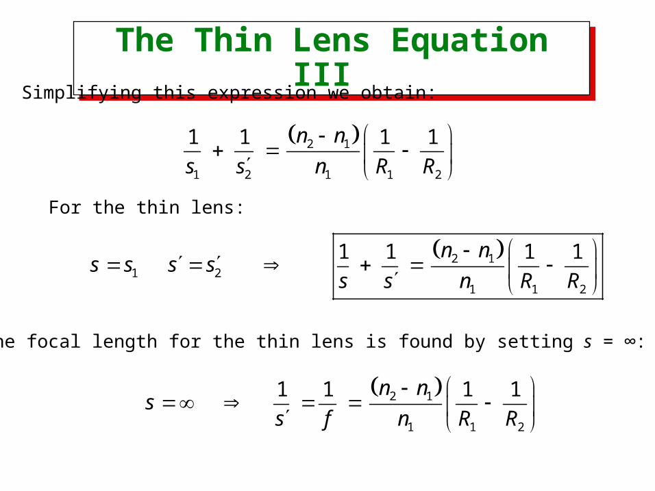
The Thin Lens Equation III The Thin Lens Equation III
2 1
1 2 1 1 2
1 1 1 1n n
s s n R R
Simplifying this expression we obtain:
2 11 2
1 1 2
1 1 1 1n ns s s s
s s n R R
For the thin lens:
2 1
1 1 2
1 1 1 1n ns
s f n R R
The focal length for the thin lens is found by setting s = ∞:
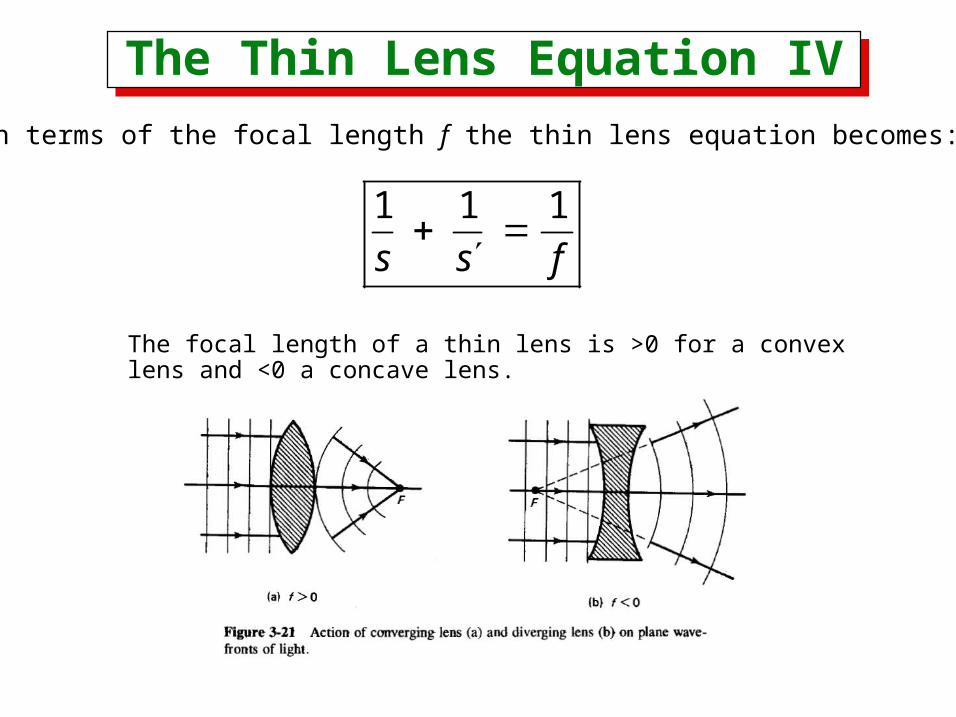
The Thin Lens Equation IV The Thin Lens Equation IV
In terms of the focal length f the thin lens equation becomes:
1 1 1
s s f
The focal length of a thin lens is >0 for a convex lens and <0 a concave lens.
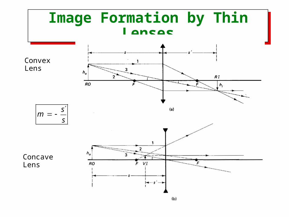
Image Formation by Thin LensesImage Formation by Thin Lenses
Convex Lens
Concave Lens
sm
s
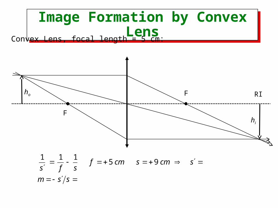
Image Formation by Convex LensImage Formation by Convex Lens
Convex Lens, focal length = 5 cm:
1 1 15 9f cm s cm s
s f s
m s s
F
F
ho
hi
RI
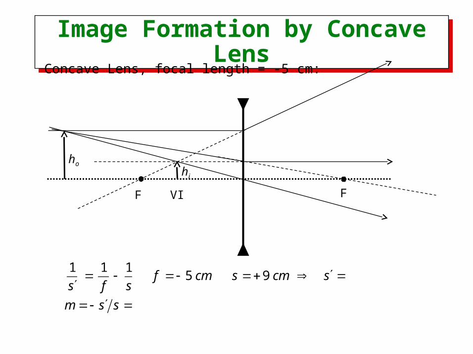
Image Formation by Concave LensImage Formation by Concave Lens
Concave Lens, focal length = -5 cm:
1 1 15 9f cm s cm s
s f s
m s s
FF
hohi
VI
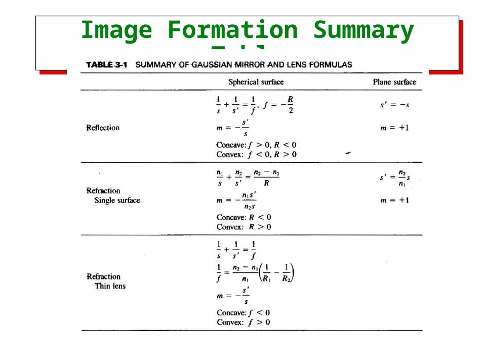
Image Formation Summary TableImage Formation Summary Table
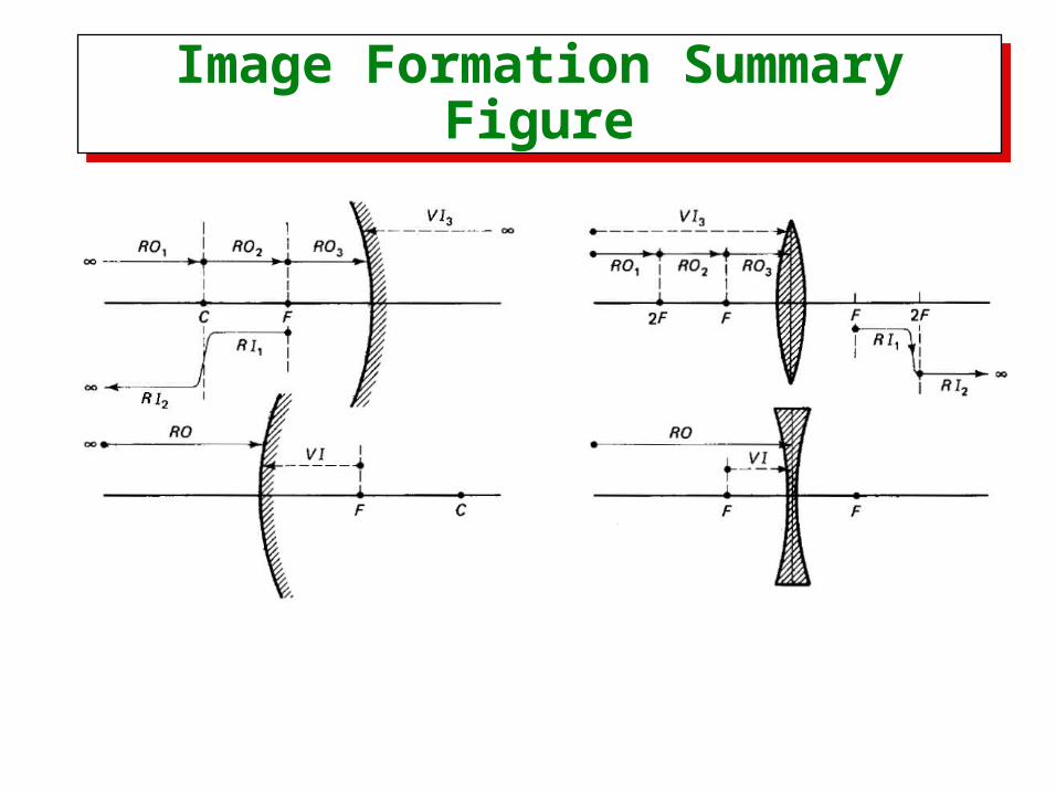
Image Formation Summary FigureImage Formation Summary Figure
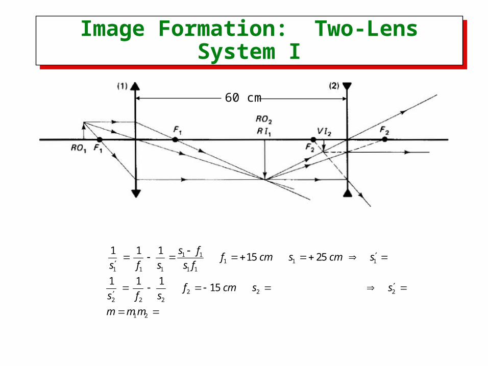
Image Formation: Two-Lens System IImage Formation: Two-Lens System I
1 11 1 1
1 1 1 1 1
2 2 22 2 2
1 2
1 1 115 25
1 1 115
s ff cm s cm s
s f s s f
f cm s ss f s
m m m
60 cm
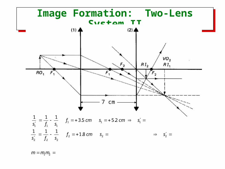
Image Formation: Two-Lens System IIImage Formation: Two-Lens System II
1 1 11 1 1
2 2 22 2 2
1 2
1 1 13.5 5.2
1 1 11.8
f cm s cm ss f s
f cm s ss f s
m m m
7 cm
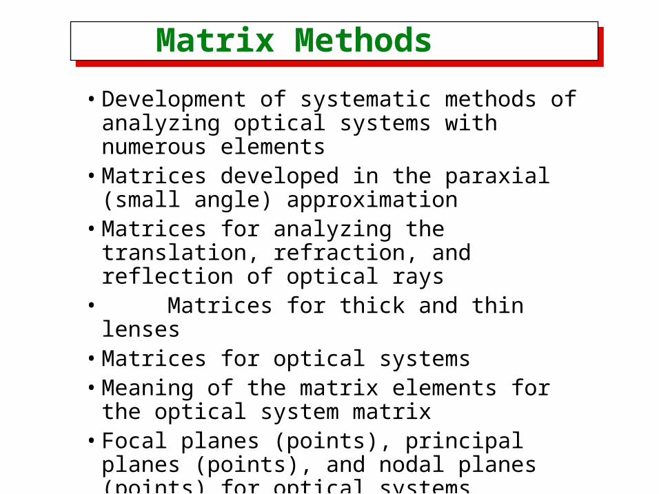
Matrix Methods Matrix Methods
• Development of systematic methods of analyzing optical systems with numerous elements
• Matrices developed in the paraxial (small angle) approximation
• Matrices for analyzing the translation, refraction, and reflection of optical rays
• Matrices for thick and thin lenses• Matrices for optical systems• Meaning of the matrix elements for the optical
system matrix• Focal planes (points), principal planes (points), and
nodal planes (points) for optical systems• Matrix analysis of optical systems
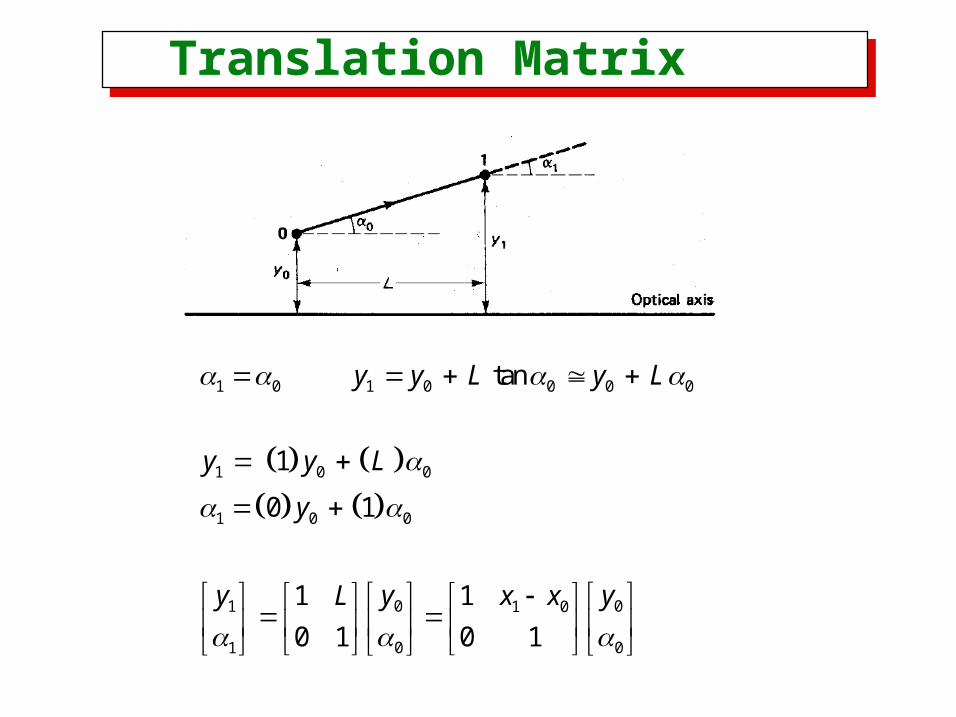
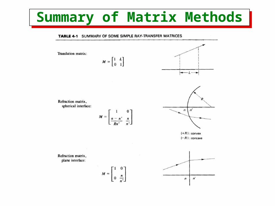
Translation Matrix Translation Matrix
1 0 1 0 0 0 0
1 0 0
1 0 0
0 01 1 0
0 01
tan
1
0 1
1 1
0 1 0 1
y y L y L
y y L
y
y yy L x x
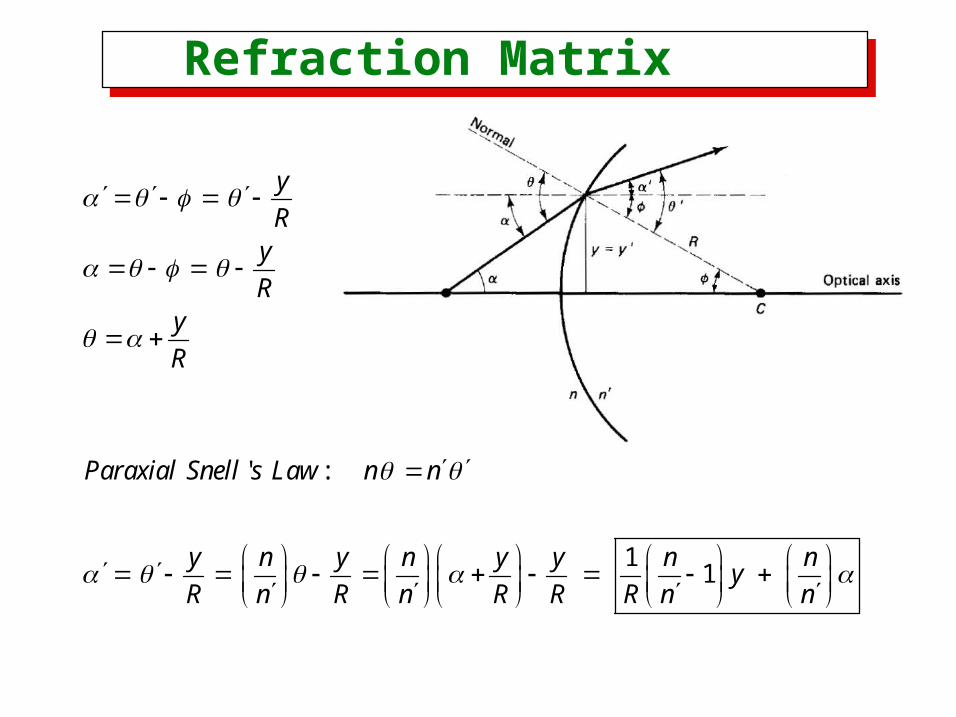
Refraction Matrix Refraction Matrix
' :
11
y
Ry
Ry
R
Paraxial Snell s Law n n
y n y n y y n ny
R n R n R R R n n
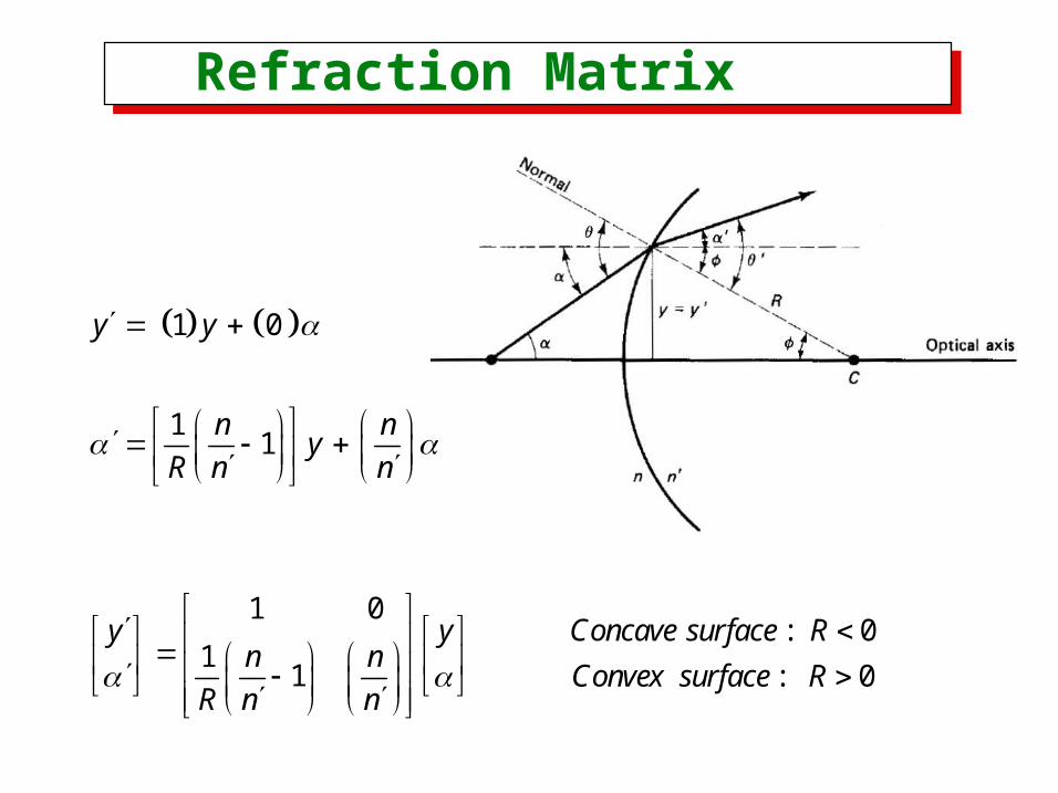
Refraction Matrix Refraction Matrix
1 0
11
1 0: 0
11 : 0
y y
n ny
R n n
y y Concave surface Rn n
Convex surface RR n n
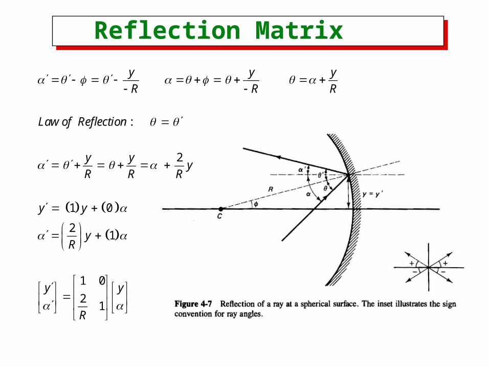
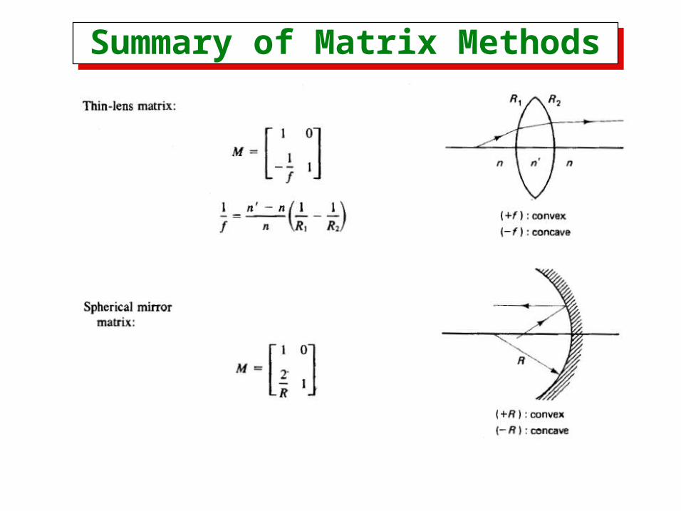
Reflection Matrix Reflection Matrix
:
2
1 0
21
1 0
21
y y y
R R R
Law of Reflection
y yy
R R R
y y
yR
y y
R
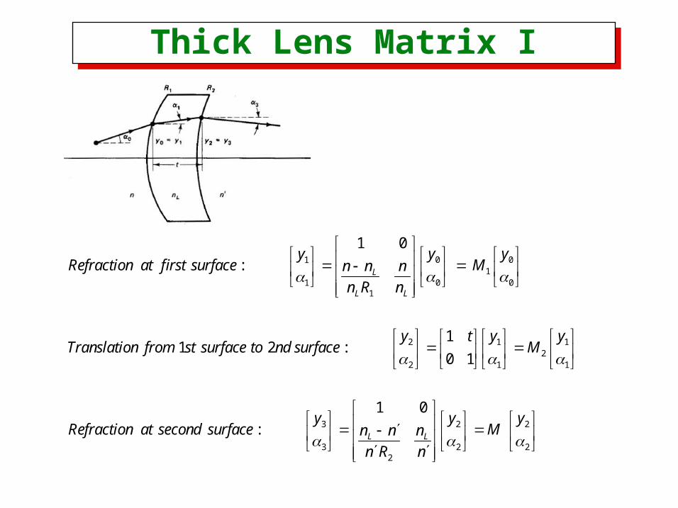
Thick Lens Matrix IThick Lens Matrix I
0 011
0 011
2 1 12
2 1 1
3
3
1 0
:
11 2 :
0 1
:
L
L L
y yyRefraction at first surface Mn n n
n R n
y y ytTranslation from st surface to nd surface M
yRefraction at second surface
2 2
2 22
1 0
L L
y yMn n n
n R n
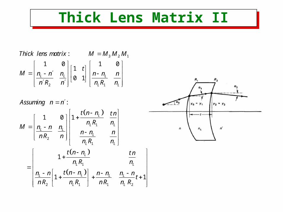
Thick Lens Matrix IIThick Lens Matrix II
3 2 1
2 1
1
21
1
2 1
:
1 0 1 01
0 1
:
11 0
1
1
L L L
L L
L
L LL L
L
L L
L
L L
LL
L
Thick lens matrix M M M M
tM n n n n n n
n R n n R n
Assuming n n
t n n t n
n R nM n n n
n n nn R n
n R n
t n n t n
n R n
t n nn n
n R n R
1 2
1L L
L
n n n nt
n R n R
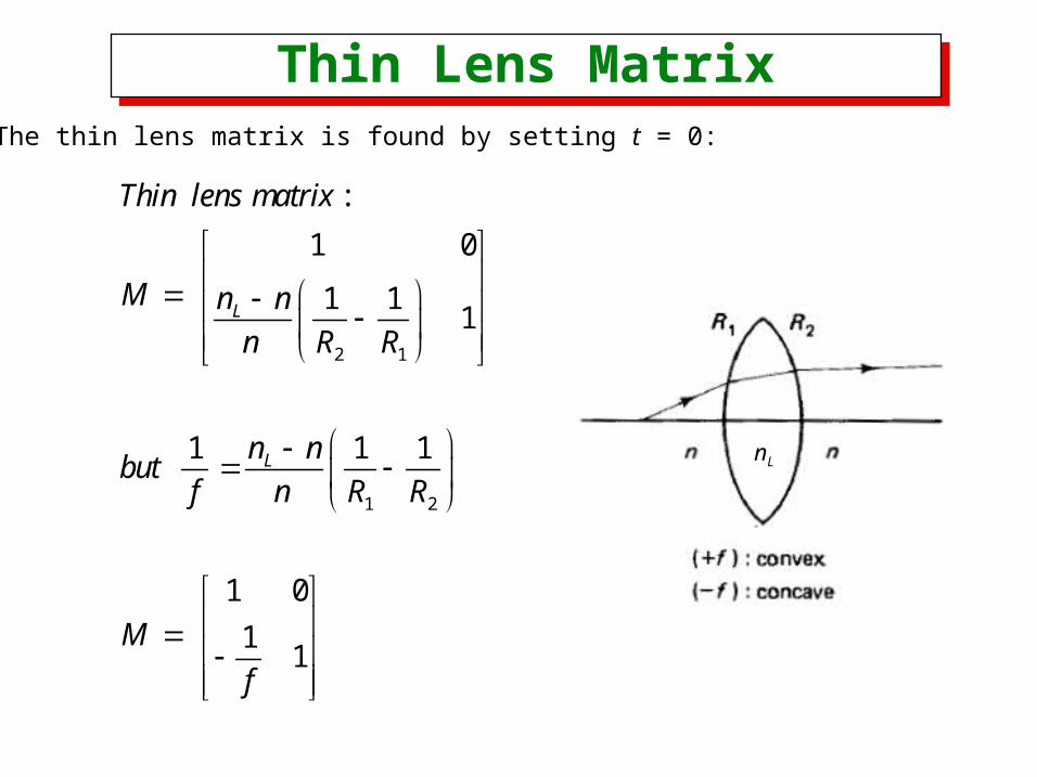
Thin Lens MatrixThin Lens Matrix
2 1
1 2
:
1 0
1 11
1 1 1
1 0
11
L
L
Thin lens matrix
M n n
n R R
n nbut
f n R R
M
f
The thin lens matrix is found by setting t = 0:
nL

Summary of Matrix MethodsSummary of Matrix Methods

Summary of Matrix MethodsSummary of Matrix Methods
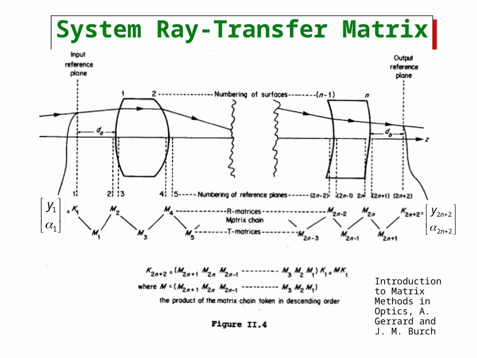
System Ray-Transfer Matrix System Ray-Transfer Matrix
Introduction to Matrix Methods in Optics, A. Gerrard and J. M. Burch
1
1
y
2 2
2 2
n
n
y
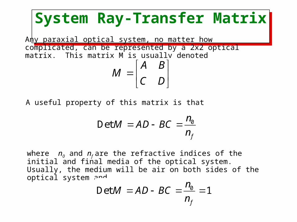
System Ray-Transfer Matrix System Ray-Transfer Matrix Any paraxial optical system, no matter how complicated, can be represented by a 2x2 optical matrix. This matrix M is usually denoted
A BM
C D
A useful property of this matrix is that
0Detf
nM AD BC
n
where n0 and nf are the refractive indices of the initial and final media of the optical system. Usually, the medium will be air on both sides of the optical system and
0Det 1f
nM AD BC
n
Summary of Matrix MethodsSummary of Matrix Methods
Summary of Matrix MethodsSummary of Matrix Methods
System Ray-Transfer Matrix System Ray-Transfer Matrix
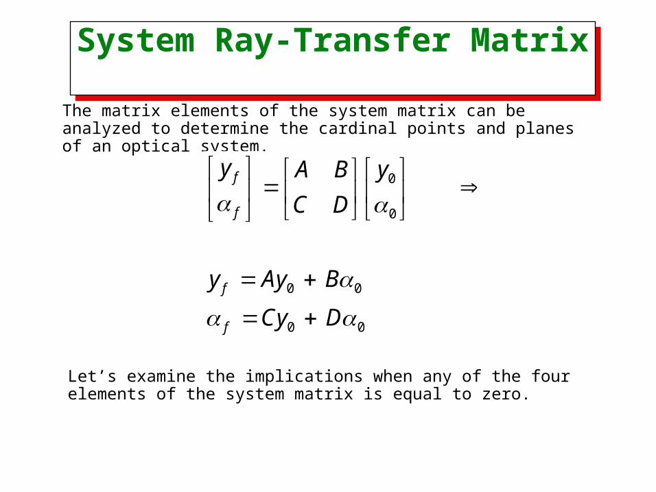
The matrix elements of the system matrix can be analyzed to determine the cardinal points and planes of an optical system.
0
0
0 0
0 0
f
f
f
f
y yA B
C D
y Ay B
Cy D
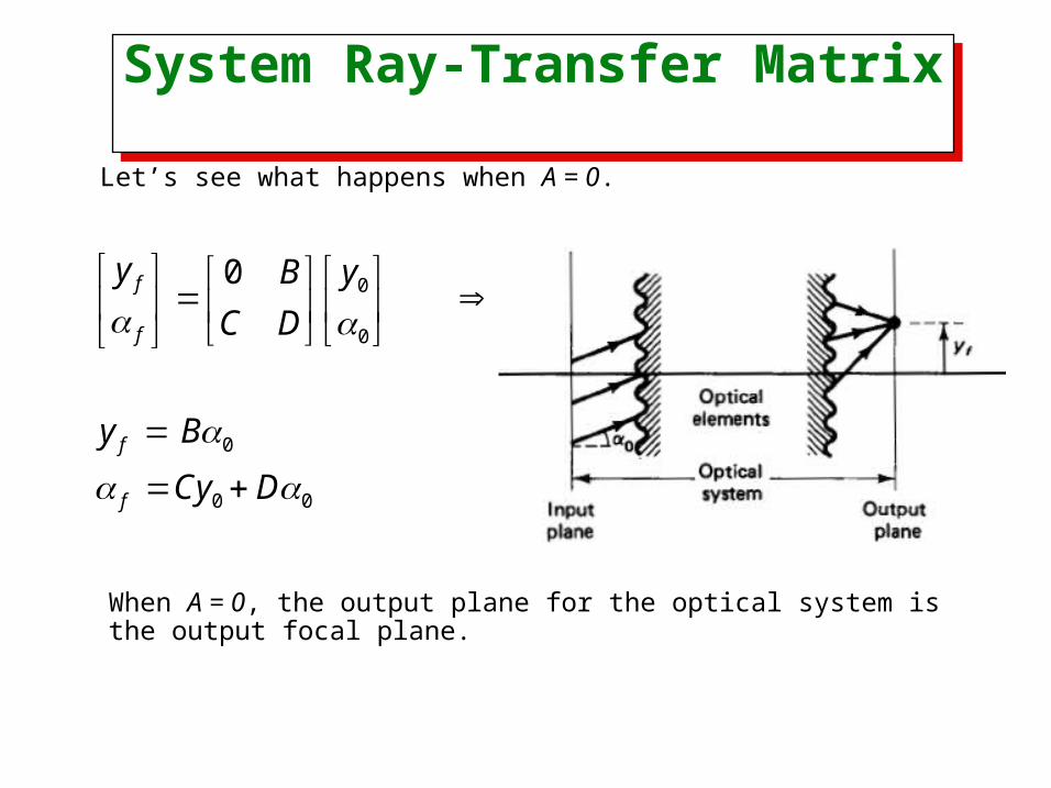
Let’s examine the implications when any of the four elements of the system matrix is equal to zero.
System Ray-Transfer Matrix System Ray-Transfer Matrix
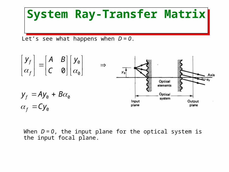
Let’s see what happens when D = 0.
0
0
0 0
0
0f
f
f
f
y yA B
C
y Ay B
Cy
When D = 0, the input plane for the optical system is the input focal plane.
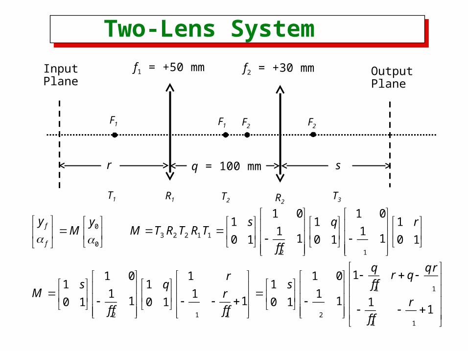
Two-Lens System Two-Lens System
f1 = +50 mm f2 = +30 mm
q = 100 mmr s
InputPlane
OutputPlane
F1 F2F1 F2
T1 R1 R2T3T2
03 2 2 1 1
02 1
1
2 1 1 2
1 0 1 01 1 1
1 11 10 1 0 1 0 1
11 0 1 1 01 1 1
1 1 11 1 10 1 0 1 0 1
f
f
y y s q rM M T R T R T
f f
q q rr qr
f fs q sM r
f f f f
1
1 1
11
r
f f
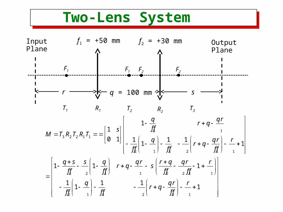
Two-Lens System Two-Lens System
f1 = +50 mm f2 = +30 mm
q = 100 mmr s
InputPlane
OutputPlane
F1 F2F1 F2
T1 R1 R2T3T2
1 1
3 2 2 1 1
2 1 1 2 1 1
1 2 1 1 2 2 1 1
2 1 1 2 1 1
11
0 1 1 1 11 1
1 1 1
1 1 11 1
q q rr q
f fsM T R T R T
q q r rr q
f f f f f f
q s s q q r r q q r rr q s
f f f f f f f f
q q r rr q
f f f f f f
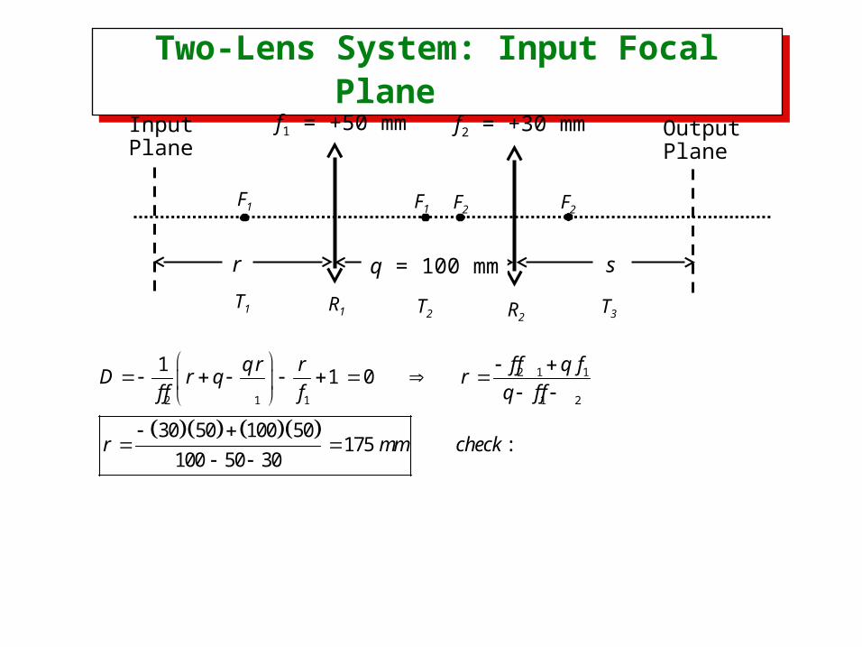
Two-Lens System: Input Focal Plane Two-Lens System: Input Focal Plane
f1 = +50 mm f2 = +30 mm
q = 100 mmr s
InputPlane
OutputPlane
F1 F2F1 F2
T1 R1 R2T3T2
2 1 1
2 1 1 1 2
11 0
30 50 100 50175 :
100 50 30
f f q fq r rD r q r
f f f q f f
r mm check
System Ray-Transfer Matrix System Ray-Transfer Matrix
Let’s see what happens when A = 0.
0
0
0
0 0
0f
f
f
f
y yB
C D
y B
Cy D
When A = 0, the output plane for the optical system is the output focal plane.
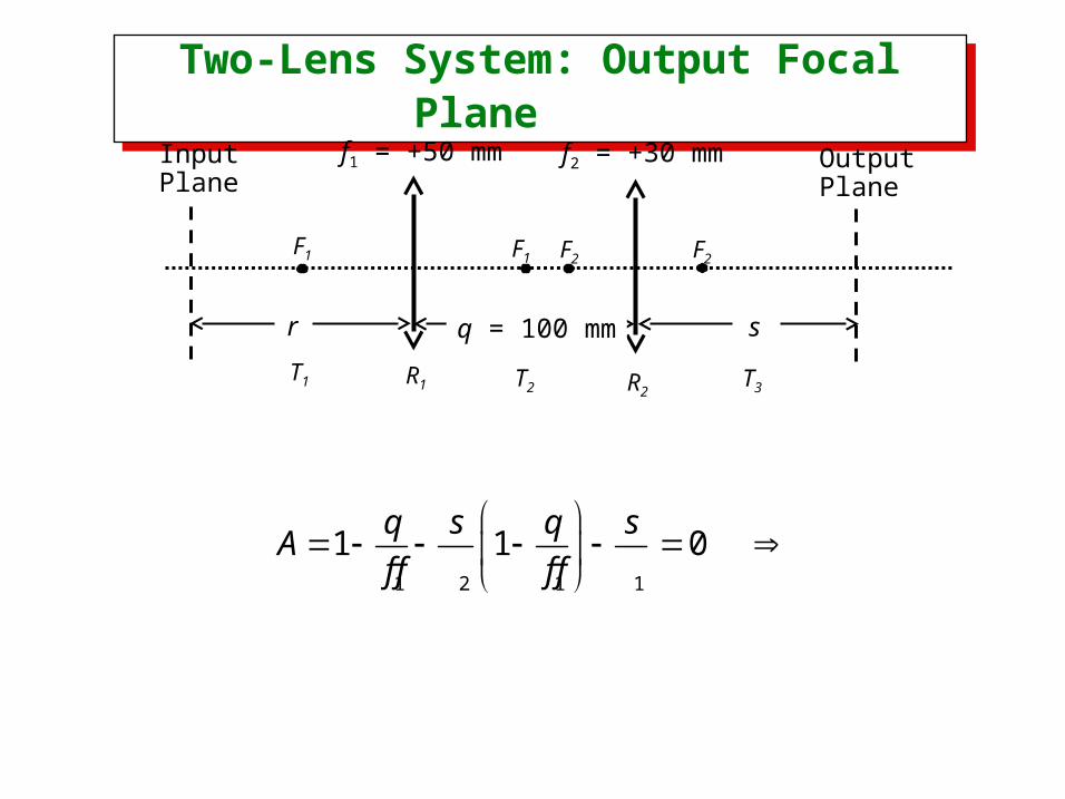
Two-Lens System: Output Focal Plane Two-Lens System: Output Focal Plane
f1 = +50 mm f2 = +30 mm
q = 100 mmr s
InputPlane
OutputPlane
F1 F2F1 F2
T1 R1 R2T3T2
1 2 1 1
1 1 0q s q s
Af f f f
System Ray-Transfer Matrix System Ray-Transfer Matrix
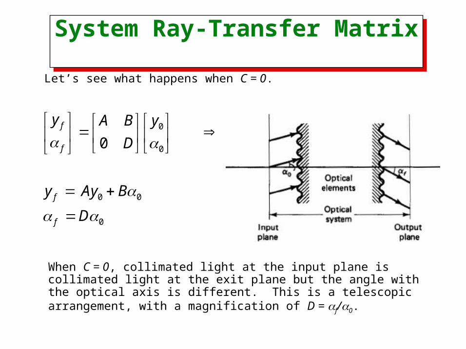
Let’s see what happens when C = 0.
0
0
0 0
0
0f
f
f
f
y yA B
D
y Ay B
D
When C = 0, collimated light at the input plane is collimated light at the exit plane but the angle with the optical axis is different. This is a telescopic arrangement, with a magnification of D = f/0.
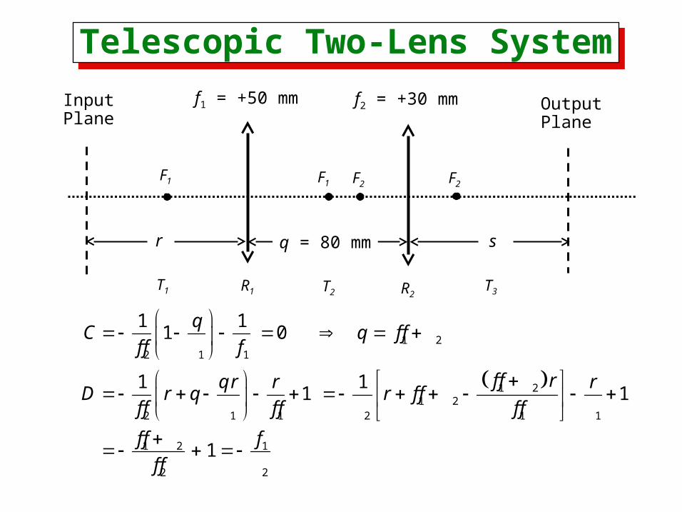
f1 = +50 mm f2 = +30 mm
q = 80 mmr s
InputPlane
OutputPlane
F1 F2F1 F2
T1 R1 R2T3T2
1 22 1 1
1 21 2
2 1 1 2 1 1
1 2 1
2 2
1 11 0
1 11 1
1
qC q f f
f f f
f f rq r r rD r q r f f
f f f f f f
f f f
f f
Telescopic Two-Lens SystemTelescopic Two-Lens System
System Ray-Transfer Matrix System Ray-Transfer Matrix
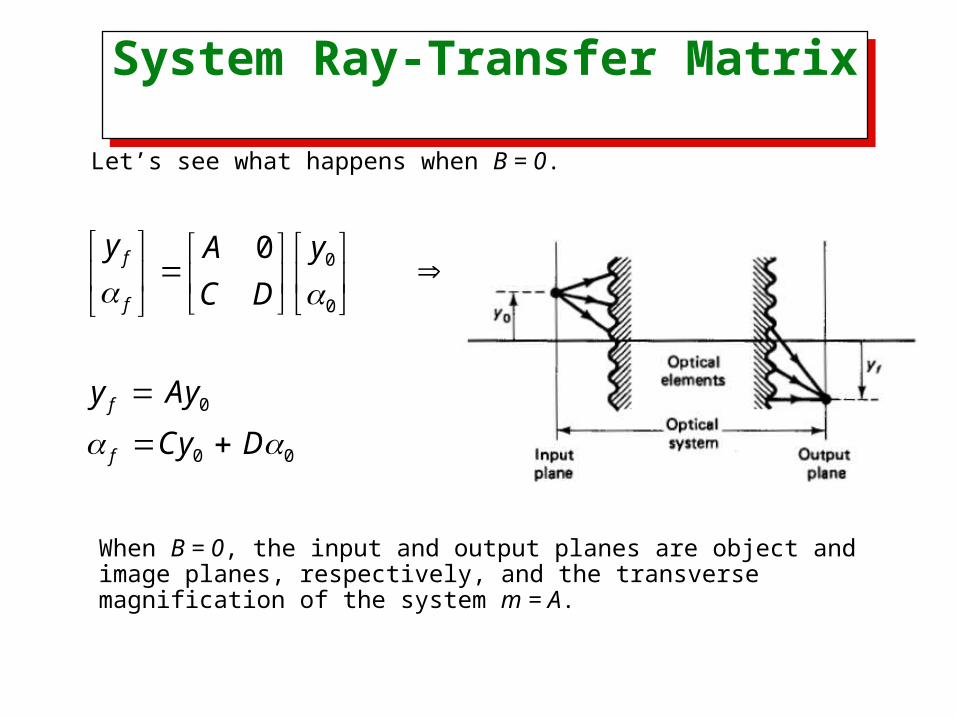
Let’s see what happens when B = 0.
0
0
0
0 0
0f
f
f
f
y yA
C D
y Ay
Cy D
When B = 0, the input and output planes are object and image planes, respectively, and the transverse magnification of the system m = A.
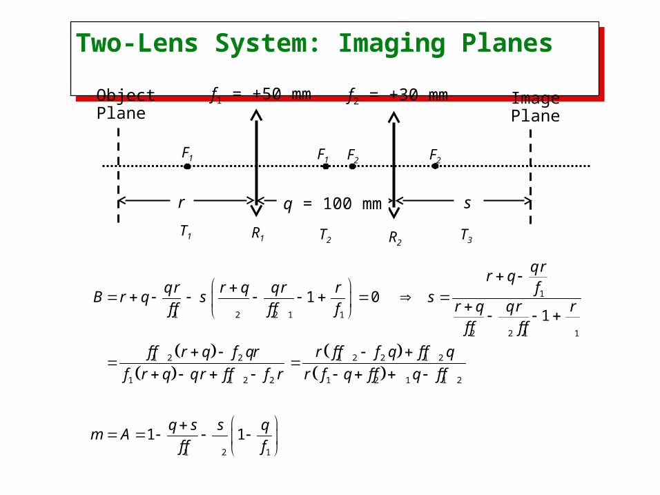
Two-Lens System: Imaging Planes Two-Lens System: Imaging Planes
f1 = +50 mm f2 = +30 mm
q = 100 mmr s
ObjectPlane
ImagePlane
F1 F2F1 F2
T1 R1 R2T3T2
1
1 2 2 1 1
2 2 1 1
1 2 2 1 2 2 1 2
1 1 2 2 1 2 1 1 2
1 2 1
1 01
1 1
q rr q
q r r q q r r fB r q s s
r q q r rf f f f ff f f f
f f r q f qr r f f f q f f q
f r q q r f f f r r f q f f q f f
q s s qm A
f f f
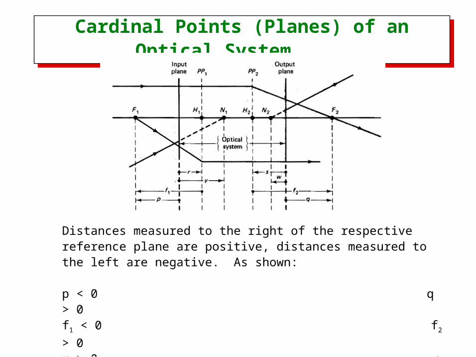
Cardinal Points (Planes) of an Optical System
Cardinal Points (Planes) of an Optical System
Distances measured to the right of the respective reference plane are positive, distances measured to the left are negative. As shown:
p < 0 q > 0 f1 < 0 f2 > 0
r > 0 s < 0v > 0 w < 0
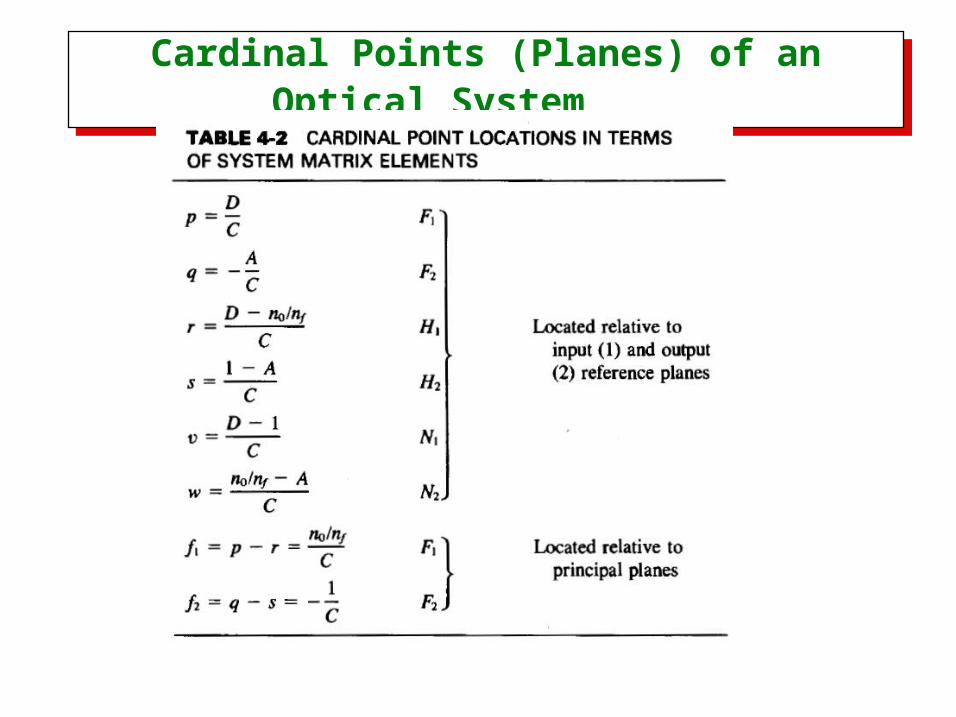
Cardinal Points (Planes) of an Optical System
Cardinal Points (Planes) of an Optical System
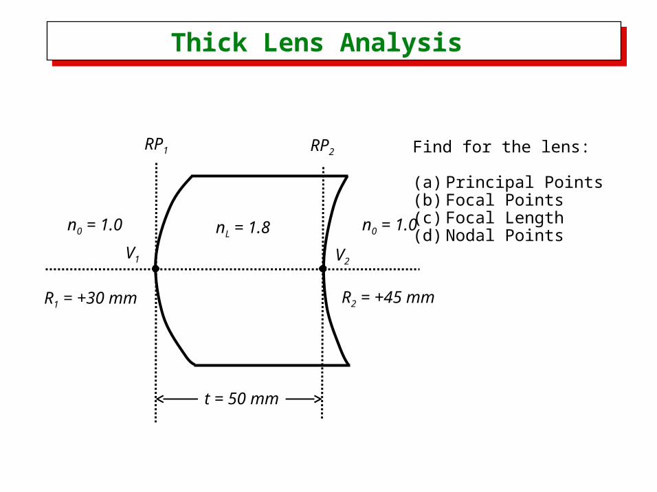
Thick Lens Analysis Thick Lens Analysis
R1 = +30 mm R2 = +45 mm
RP1 RP2
V1 V2
t = 50 mm
nL = 1.8n0 = 1.0 n0 = 1.0
Find for the lens:
(a) Principal Points(b) Focal Points(c) Focal Length(d) Nodal Points
1
2 1 1 2
, :
1
1 1
50* 0.8 50*1.01
1.8*30 1.8
50* 0.80.8 0.8 0.8*501 1
45 1.8*30 30 1.8*45
L
L L
LL L L
L L
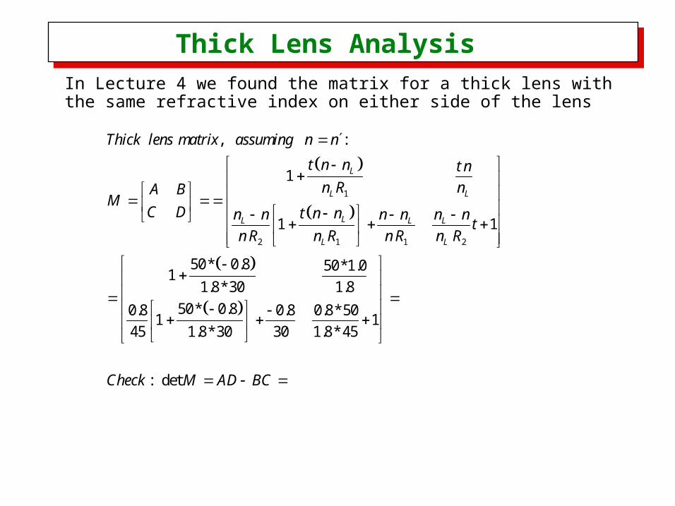
Thick lens matrix assuming n n
t n n t n
n R nA BM
C D t n nn n n n n nt
n R n R n R n R
: detCheck M AD BC
Thick Lens Analysis Thick Lens Analysis In Lecture 4 we found the matrix for a thick lens with the same refractive index on either side of the lens
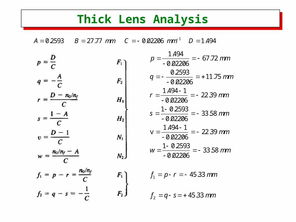
10.2593 27.77 0.02206 1.494A B mm C mm D
Thick Lens Analysis Thick Lens Analysis
1
2
1.49467.72
0.022060.2593
11.750.02206
1.494 122.39
0.022061 0.2593
33.580.022061.494 1
v 22.390.022061 0.2593
33.580.02206
45.33
45.33
p mm
q mm
r mm
s mm
mm
w mm
f p r mm
f q s mm
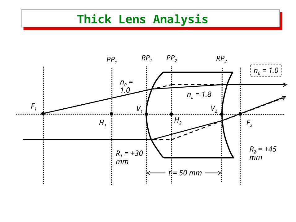
Thick Lens Analysis Thick Lens Analysis
R1 = +30 mm
R2 = +45 mm
RP1 RP2
V1 V2
t = 50 mm
nL = 1.8
n0 = 1.0
n0 = 1.0
PP1
F1
F2
PP2
H1H2
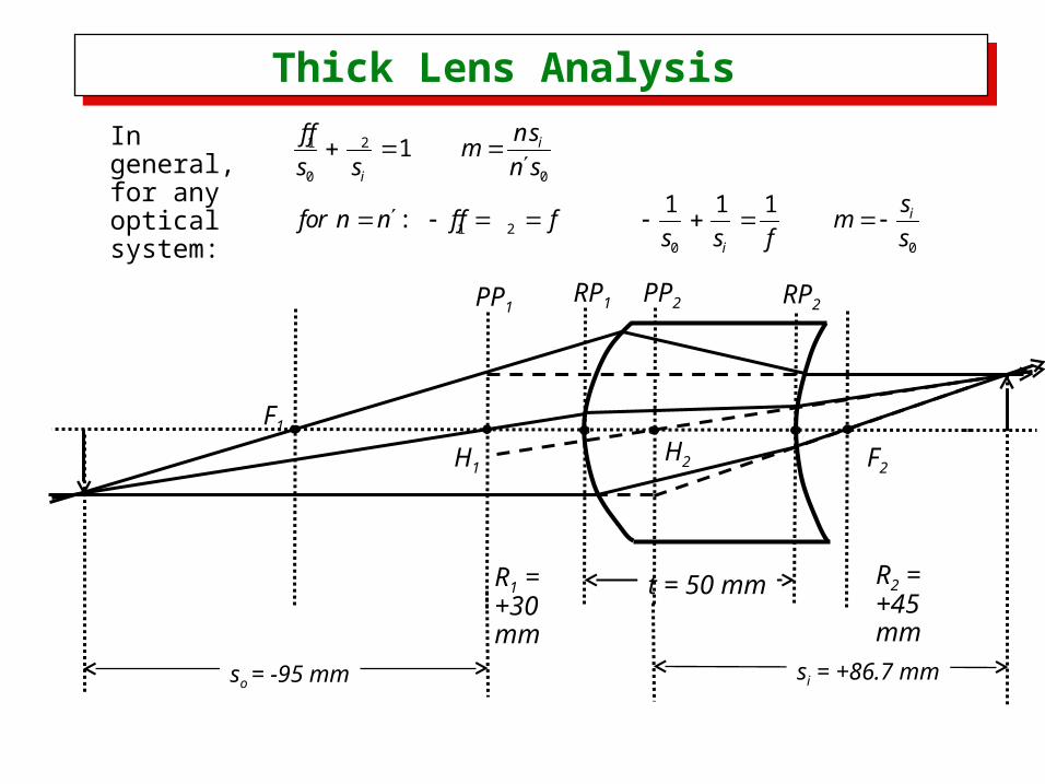
Thick Lens Analysis Thick Lens Analysis
R1 = +30 mm
R2 = +45 mm
RP1 RP2
t = 50 mm
PP1
F1
F2
PP2
H1H2
si = +86.7 mmso = -95 mm
In general, for any optical system:
1 2
0 0
1 20 0
1
1 1 1:
i
i
i
i
n sf fm
s s n s
sfor n n f f f m
s s f s