Proceedings of the 6th Workshop on Computational Approaches to Subjectivity, Sentiment and Social Media Analysis (WASSA 2015), pages 16–24,Lisboa, Portugal, 17 September, 2015. c©2015 Association for Computational Linguistics.

Enhanced Twitter Sentiment Classification Using Contextual Information

Soroush VosoughiThe Media Lab

MITCambridge, MA 02139

soroush@mit.edu

Helen ZhouThe Media Lab

MITCambridge, MA 02139

hlzhou@mit.edu

Deb RoyThe Media Lab

MITCambridge, MA 02139dkroy@media.mit.edu

Abstract

The rise in popularity and ubiquity ofTwitter has made sentiment analysis oftweets an important and well-covered areaof research. However, the 140 characterlimit imposed on tweets makes it hard touse standard linguistic methods for sen-timent classification. On the other hand,what tweets lack in structure they make upwith sheer volume and rich metadata. Thismetadata includes geolocation, temporaland author information. We hypothesizethat sentiment is dependent on all thesecontextual factors. Different locations,times and authors have different emotionalvalences. In this paper, we explored thishypothesis by utilizing distant supervisionto collect millions of labelled tweets fromdifferent locations, times and authors. Weused this data to analyse the variation oftweet sentiments across different authors,times and locations. Once we exploredand understood the relationship betweenthese variables and sentiment, we used aBayesian approach to combine these vari-ables with more standard linguistic fea-tures such as n-grams to create a Twit-ter sentiment classifier. This combinedclassifier outperforms the purely linguis-tic classifier, showing that integrating therich contextual information available onTwitter into sentiment classification is apromising direction of research.

1 Introduction

Twitter is a micro-blogging platform and a socialnetwork where users can publish and exchangeshort messages of up to 140 characters long (alsoknown as tweets). Twitter has seen a great rise inpopularity in recent years because of its availabil-ity and ease-of-use. This rise in popularity and the

public nature of Twitter (less than 10% of Twitteraccounts are private (Moore, 2009)) have made itan important tool for studying the behaviour andattitude of people.

One area of research that has attracted great at-tention in the last few years is that of tweet sen-timent classification. Through sentiment classifi-cation and analysis, one can get a picture of peo-ple’s attitudes about particular topics on Twitter.This can be used for measuring people’s attitudestowards brands, political candidates, and social is-sues.

There have been several works that do senti-ment classification on Twitter using standard sen-timent classification techniques, with variations ofn-gram and bag of words being the most common.There have been attempts at using more advancedsyntactic features as is done in sentiment classifi-cation for other domains (Read, 2005; Nakagawaet al., 2010), however the 140 character limit im-posed on tweets makes this hard to do as each arti-cle in the Twitter training set consists of sentencesof no more than several words, many of them withirregular form (Saif et al., 2012).

On the other hand, what tweets lack in structurethey make up with sheer volume and rich meta-data. This metadata includes geolocation, tempo-ral and author information. We hypothesize thatsentiment is dependent on all these contextual fac-tors. Different locations, times and authors havedifferent emotional valences. For instance, peo-ple are generally happier on weekends and cer-tain hours of the day, more depressed at the endof summer holidays, and happier in certain statesin the United States. Moreover, people have differ-ent baseline emotional valences from one another.These claims are supported for example by the an-nual Gallup poll that ranks states from most happyto least happy (Gallup-Healthways, 2014), or thework by Csikszentmihalyi and Hunter (Csikszent-mihalyi and Hunter, 2003) that showed reported

16

happiness varies significantly by day of week andtime of day. We believe these factors manifestthemselves in sentiments expressed in tweets andthat by accounting for these factors, we can im-prove sentiment classification on Twitter.

In this work, we explored this hypothesis by uti-lizing distant supervision (Go et al., 2009) to col-lect millions of labelled tweets from different lo-cations (within the USA), times of day, days ofthe week, months and authors. We used this datato analyse the variation of tweet sentiments acrossthe aforementioned categories. We then used aBayesian approach to incorporate the relationshipbetween these factors and tweet sentiments intostandard n-gram based Twitter sentiment classifi-cation.

This paper is structured as follows. In the nextsections we will review related work on sentimentclassification, followed by a detailed explanationof our approach and our data collection, annota-tion and processing efforts. After that, we describeour baseline n-gram sentiment classifier model,followed by the explanation of how the baselinemodel is extended to incorporate contextual in-formation. Next, we describe our analysis of thevariation of sentiment within each of the contex-tual categories. We then evaluate our models andfinally summarize our findings and contributionsand discuss possible paths for future work.

2 Related Work

Sentiment analysis and classification of text is aproblem that has been well studied across manydifferent domains, such as blogs, movie reviews,and product reviews (e.g., (Pang et al., 2002; Cuiet al., 2006; Chesley et al., 2006)). There is alsoextensive work on sentiment analysis for Twitter.Most of the work on Twitter sentiment classifica-tion either focuses on different machine learningtechniques (e.g., (Wang et al., 2011; Jiang et al.,2011)), novel features (e.g., (Davidov et al., 2010;Kouloumpis et al., 2011; Saif et al., 2012)), newdata collection and labelling techniques (e.g., (Goet al., 2009)) or the application of sentiment clas-sification to analyse the attitude of people aboutcertain topics on Twitter (e.g., (Diakopoulos andShamma, 2010; Bollen et al., 2011)). These arejust some examples of the extensive research al-ready done on Twitter sentiment classification andanalysis.

There has also been previous work on measur-

ing the happiness of people in different contexts(location, time, etc). This has been done mostlythrough traditional land-line polling (Csikszent-mihalyi and Hunter, 2003; Gallup-Healthways,2014), with Gallup’s annual happiness index be-ing a prime example (Gallup-Healthways, 2014).More recently, some have utilized Twitter to mea-sure people’s mood and happiness and have foundTwitter to be a generally good measure of the pub-lic’s overall happiness, well-being and mood. Forexample, Bollen et al. (Bollen et al., 2011) usedTwitter to measure the daily mood of the pub-lic and compare that to the record of social, po-litical, cultural and economic events in the realworld. They found that these events have a sig-nificant effect on the public mood as measuredthrough Twitter. Another example would be thework of Mitchell et al. (Mitchell et al., 2013), inwhich they estimated the happiness levels of dif-ferent states and cities in the USA using Twitterand found statistically significant correlations be-tween happiness level and the demographic char-acteristics (such as obesity rates and education lev-els) of those regions.

In this work, we combined the sentiment anal-ysis of different authors, locations, times anddates as measured through labelled Twitter datawith standard word-based sentiment classificationmethods to create a context-dependent sentimentclassifier. As far as we can tell, there has notbeen significant previous work on Twitter senti-ment classification that has achieved this.

3 Approach

The main hypothesis behind this work is that theaverage sentiment of messages on Twitter is dif-ferent in different contexts. Specifically, tweets indifferent spatial, temporal and authorial contextshave on average different sentiments. Basically,these factors (many of which are environmental)have an affect on the emotional states of peoplewhich in turn have an effect on the sentiments peo-ple express on Twitter and elsewhere. In this pa-per, we used this contextual information to betterpredict the sentiment of tweets.

Luckily, tweets are tagged with very rich meta-data, including location, timestamp, and author in-formation. By analysing labelled data collectedfrom these different contexts, we calculated priorprobabilities of negative and positive sentimentsfor each of the contextual categories shown below:

17

• The states in the USA (50 total).

• Hour of the day (HoD) (24 total).

• Day of week (DoW) (7 total).

• Month (12 total).

• Authors (57710 total).

This means that for every item in each of thesecategories, we calculated a probability of senti-ment being positive or negative based on histori-cal tweets. For example, if seven out of ten his-torical tweets made on Friday were positive thenthe prior probability of a sentiment being positivefor tweets sent out on Friday is 0.7 and the priorprobability of a sentiment being negative is 0.3.We then trained a Bayesian sentiment classifier us-ing a combination of these prior probabilities andstandard n-gram models. The model is describedin great detail in the ”Baseline Model” and ”Con-textual Model” sections of this paper.

In order to do a comprehensive analysis of sen-timent of tweets across aforementioned contex-tual categories, a large amount of labelled datawas required. We needed thousands of tweets forevery item in each of the categories (e.g. thou-sands of tweets per hour of day, or state in theUS). Therefore, creating a corpus using human-annotated data would have been impractical. In-stead, we turned to distant supervision techniquesto obtain our corpus. Distant supervision allowsus to have noisy but large amounts of annotatedtweets.

There are different methods of obtaining la-belled data using distant supervision (Read, 2005;Go et al., 2009; Barbosa and Feng, 2010; Davidovet al., 2010). We used emoticons to label tweetsas positive or negative, an approach that was in-troduced by Read (Read, 2005) and used in multi-ple works (Go et al., 2009; Davidov et al., 2010).We collected millions of English-language tweetsfrom different times, dates, authors and US states.We used a total of six emoticons, three mappingto positive and three mapping to negative senti-ment (table 1). We identified more than 120 pos-itive and negative ASCII emoticons and unicodeemojis1, but we decided to only use the six mostcommon emoticons in order to avoid possible se-lection biases. For example, people who use ob-scure emoticons and emojis might have a differ-ent base sentiment from those who do not. Using

1Japanese pictographs similar to ASCII emoticons

the six most commonly used emoticons limits thisbias. Since there are no ”neutral” emoticons, ourdataset is limited to tweets with positive or nega-tive sentiments. Accordingly, in this work we areonly concerned with analysing and classifying thepolarity of tweets (negative vs. positive) and nottheir subjectivity (neutral vs. non-neutral). Belowwe will explain our data collection and corpus ingreater detail.

Positive Emoticons Negative Emoticons:) :(:-) :-(: ) : (

Table 1: List of emoticons.

4 Data Collection and Datasets

We collected two datasets, one massive and la-belled through distant supervision, the other smalland labelled by humans. The massive dataset wasused to calculate the prior probabilities for eachof our contextual categories. Both datasets wereused to train and test our sentiment classifier. Thehuman-labelled dataset was used as a sanity checkto make sure the dataset labelled using the emoti-cons classifier was not too noisy and that the hu-man and emoticon labels matched for a majorityof tweets.

4.1 Emoticon-based Labelled DatasetWe collected a total of 18 million, geo-tagged,English-language tweets over three years, fromJanuary 1st, 2012 to January 1st, 2015, evenly di-vided across all 36 months, using Historical Pow-erTrack for Twitter2 provided by GNIP3. We cre-ated geolocation bounding boxes4 for each of the50 states which were used to collect our dataset.All 18 million tweets originated from one of the50 states and are tagged as such. Moreover, alltweets contained one of the six emoticons in Ta-ble 1 and were labelled as either positive or nega-tive based on the emoticon. Out of the 18 milliontweets, 11.2 million (62%) were labelled as posi-tive and 6.8 million (38%) were labelled as nega-tive. The 18 million tweets came from 7, 657, 158distinct users.

2Historical PowerTrack for Twitter provides complete ac-cess to the full archive of Twitter public data.

3https://gnip.com/4The bounding boxes were created using

http://boundingbox.klokantech.com/

18

4.2 Human Labelled DatasetWe randomly selected 3000 tweets from our largedataset and had all their emoticons stripped. Wethen had these tweets labelled as positive or neg-ative by three human annotators. We measuredthe inter-annotator agreement using Fleiss’ kappa,which calculates the degree of agreement in clas-sification over that which would be expected bychance (Fleiss, 1971). The kappa score for thethree annotators was 0.82, which means that therewere disagreements in sentiment for a small por-tion of the tweets. However, the number of tweetsthat were labelled the same by at least two of thethree human annotator was 2908 out of of the 3000tweets (96%). Of these 2908 tweets, 60% were la-belled as positive and 40% as negative.

We then measured the agreement between thehuman labels and emoticon-based labels, usingonly tweets that were labelled the same by at leasttwo of the three human annotators (the majoritylabel was used as the label for the tweet). Table2 shows the confusion matrix between human andemoticon-based annotations. As you can see, 85%of all labels matched ( 1597+822

1597+882+281+148 = .85).

Human-Pos Human-NegEmot-Pos 1597 281Emot-Neg 148 882

Table 2: Confusion matrix between human-labelled and emoticon-labelled tweets.

These results are very promising and show thatusing emoticon-based distant supervision to labelthe sentiment of tweets is an acceptable method.Though there is some noise introduced to thedataset (as evidenced by the 15% of tweets whosehuman labels did not match their emoticon la-bels), the sheer volume of labelled data that thismethod makes accessible, far outweighs the rela-tively small amount of noise introduced.

4.3 Data PreparationSince the data is labelled using emoticons, westripped all emoticons from the training data. Thisensures that emoticons are not used as a featurein our sentiment classifier. A large portion oftweets contain links to other websites. These linksare mostly not meaningful semantically and thuscan not help in sentiment classification. There-fore, all links in tweets were replaced with thetoken ”URL”. Similarly, all mentions of user-

names (which are denoted by the @ symbol) werereplaced with the token ”USERNAME”, sincethey also can not help in sentiment classification.Tweets also contain very informal language andas such, characters in words are often repeated foremphasis (e.g., the word good is used with an ar-bitrary number of o’s in many tweets). Any char-acter that was repeated more than two times wasremoved (e.g., goooood was replaced with good).Finally, all words in the tweets were stemmed us-ing Porter Stemming (Porter, 1980).

5 Baseline Model

For our baseline sentiment classification model,we used our massive dataset to train a negative andpositive n-gram language model from the negativeand positive tweets.

As our baseline model, we built purely linguis-tic bigram models in Python, utilizing some com-ponents from NLTK (Bird et al., 2009). Thesemodels used a vocabulary that was filtered to re-move words occurring 5 or fewer times. Probabil-ity distributions were calculated using Kneser-Neysmoothing (Chen and Goodman, 1999). In addi-tion to Kneser-Ney smoothing, the bigram mod-els also used “backoff” smoothing (Katz, 1987), inwhich an n-gram model falls back on an (n − 1)-gram model for words that were unobserved in then-gram context.

In order to classify the sentiment of a new tweet,its probability of fit is calculated using both thenegative and positive bigram models. Equation 1below shows our models through a Bayesian lens.

Pr(θs |W ) =Pr(W | θs) Pr(θs)

Pr(W )(1)

Here θs can be θp or θn, corresponding to thehypothesis that the sentiment of the tweet is pos-itive or negative respectively. W is the sequenceof ` words, written as w`

1, that make up the tweet.Pr(W ) is not dependent on the hypothesis, andcan thus be ignored. Since we are using a bigrammodel, Equation 1 can be written as:

Pr(θs |W ) ∝∏̀i=2

Pr(wi | wi−1, θs) Pr(θs)

(2)

This is our purely linguistic baseline model.

19

6 Contextual Model

The Bayesian approach allows us to easily inte-grate the contextual information into our models.Pr(θs) in Equation 2 is the prior probability of atweet having the sentiment s. The prior probabil-ity (Pr(θs)) can be calculated using the contextualinformation of the tweets. Therefore, Pr(θs) inequation 2 is replaced by Pr(θs|C), which is theprobability of the hypothesis given the contextualinformation. Pr(θs|C) is the posterior probabilityof the following Bayesian equation:

Pr(θs | C) =Pr(C | θs) Pr(θs)

Pr(C)(3)

Where C is the set of contextual vari-ables: {State,HoD,Dow,Month,Author}.Pr(θs|C) captures the probability that a tweet ispositive or negative, given the state, hour of day,day of the week, month and author of the tweet.Here Pr(C) is not dependent on the hypothesis,and thus can be ignored. Equation 2 can thereforebe rewritten to include the contextual information:

Pr(θs |W,C) ∝∏̀i=2

Pr(wi | wi−1, θs)

Pr(C | θs) Pr(θs)

(4)

Equation 4 is our extended Bayesian model forintegrating contextual information with more stan-dard, word-based sentiment classification.

7 Sentiment in Context

We considered five contextual categories: one spa-tial, three temporal and one authorial. Here is thelist of the five categories:

• The states in the USA (50 total) (spatial).

• Hour of the day (HoD) (24 total) (temporal).

• Day of week (DoW) (7 total) (temporal).

• Month (12 total) (temporal).

• Authors (57,710 total) (authorial).

We used our massive emoticon labelled datasetto calculate the average sentiment for all of thesefive categories. A tweet was given a score of−1 ifit was labelled as negative and a score 1 if it waslabelled as positive, so an average sentiment of 0for a contextual category would mean that tweetsin that category were evenly labelled as positiveand negative.

7.1 Spatial

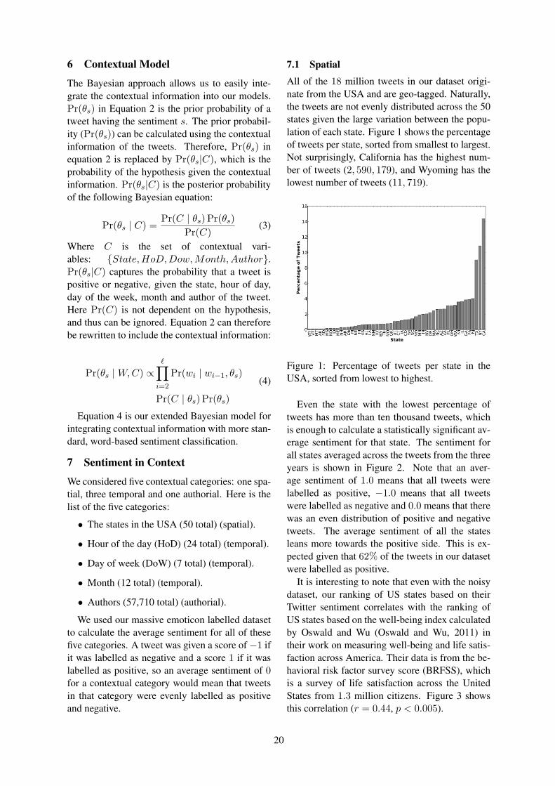
All of the 18 million tweets in our dataset origi-nate from the USA and are geo-tagged. Naturally,the tweets are not evenly distributed across the 50states given the large variation between the popu-lation of each state. Figure 1 shows the percentageof tweets per state, sorted from smallest to largest.Not surprisingly, California has the highest num-ber of tweets (2, 590, 179), and Wyoming has thelowest number of tweets (11, 719).

Figure 1: Percentage of tweets per state in theUSA, sorted from lowest to highest.

Even the state with the lowest percentage oftweets has more than ten thousand tweets, whichis enough to calculate a statistically significant av-erage sentiment for that state. The sentiment forall states averaged across the tweets from the threeyears is shown in Figure 2. Note that an aver-age sentiment of 1.0 means that all tweets werelabelled as positive, −1.0 means that all tweetswere labelled as negative and 0.0 means that therewas an even distribution of positive and negativetweets. The average sentiment of all the statesleans more towards the positive side. This is ex-pected given that 62% of the tweets in our datasetwere labelled as positive.

It is interesting to note that even with the noisydataset, our ranking of US states based on theirTwitter sentiment correlates with the ranking ofUS states based on the well-being index calculatedby Oswald and Wu (Oswald and Wu, 2011) intheir work on measuring well-being and life satis-faction across America. Their data is from the be-havioral risk factor survey score (BRFSS), whichis a survey of life satisfaction across the UnitedStates from 1.3 million citizens. Figure 3 showsthis correlation (r = 0.44, p < 0.005).

20

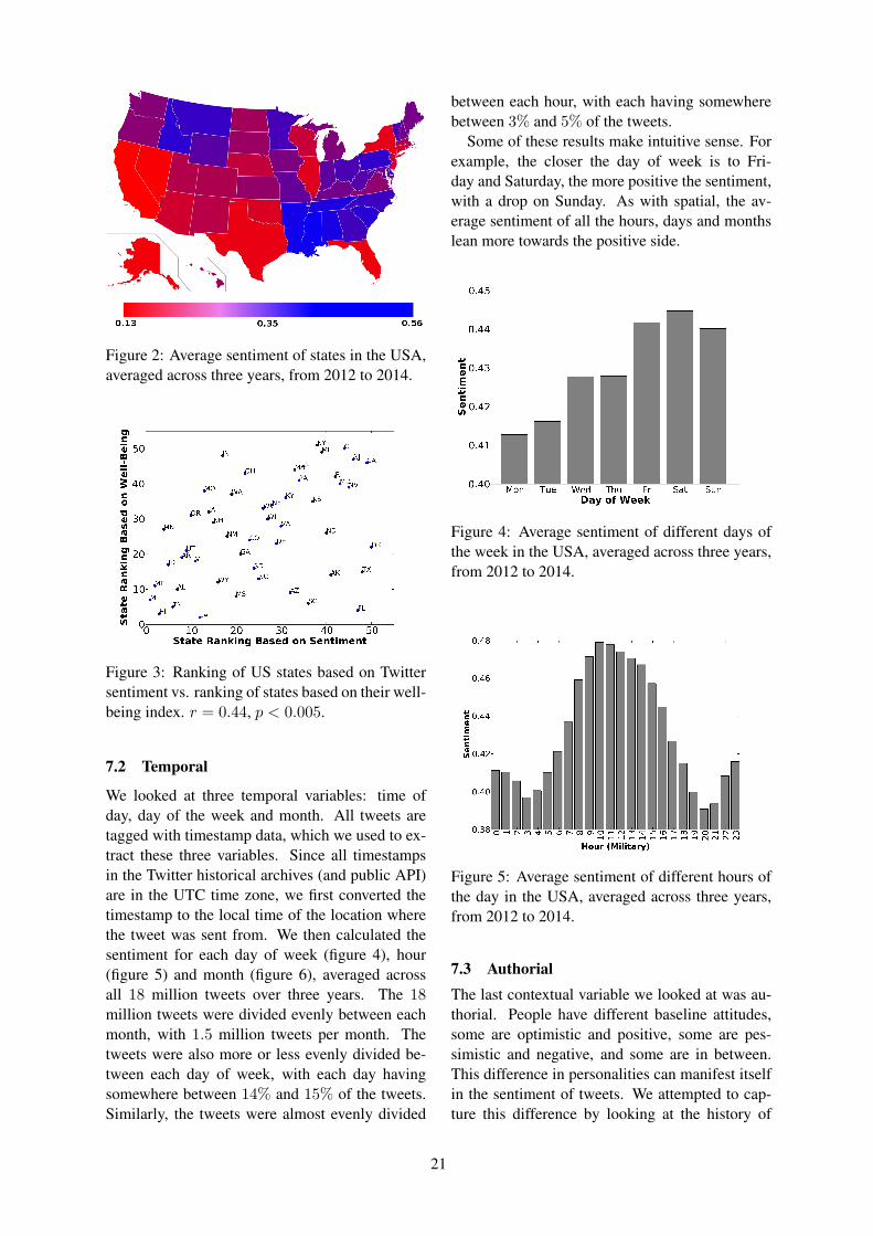
Figure 2: Average sentiment of states in the USA,averaged across three years, from 2012 to 2014.

Figure 3: Ranking of US states based on Twittersentiment vs. ranking of states based on their well-being index. r = 0.44, p < 0.005.

7.2 Temporal

We looked at three temporal variables: time ofday, day of the week and month. All tweets aretagged with timestamp data, which we used to ex-tract these three variables. Since all timestampsin the Twitter historical archives (and public API)are in the UTC time zone, we first converted thetimestamp to the local time of the location wherethe tweet was sent from. We then calculated thesentiment for each day of week (figure 4), hour(figure 5) and month (figure 6), averaged acrossall 18 million tweets over three years. The 18million tweets were divided evenly between eachmonth, with 1.5 million tweets per month. Thetweets were also more or less evenly divided be-tween each day of week, with each day havingsomewhere between 14% and 15% of the tweets.Similarly, the tweets were almost evenly divided

between each hour, with each having somewherebetween 3% and 5% of the tweets.

Some of these results make intuitive sense. Forexample, the closer the day of week is to Fri-day and Saturday, the more positive the sentiment,with a drop on Sunday. As with spatial, the av-erage sentiment of all the hours, days and monthslean more towards the positive side.

Figure 4: Average sentiment of different days ofthe week in the USA, averaged across three years,from 2012 to 2014.

Figure 5: Average sentiment of different hours ofthe day in the USA, averaged across three years,from 2012 to 2014.

7.3 AuthorialThe last contextual variable we looked at was au-thorial. People have different baseline attitudes,some are optimistic and positive, some are pes-simistic and negative, and some are in between.This difference in personalities can manifest itselfin the sentiment of tweets. We attempted to cap-ture this difference by looking at the history of

21

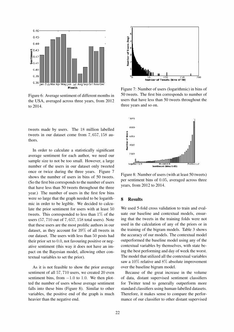
Figure 6: Average sentiment of different months inthe USA, averaged across three years, from 2012to 2014.

tweets made by users. The 18 million labelledtweets in our dataset come from 7, 657, 158 au-thors.

In order to calculate a statistically significantaverage sentiment for each author, we need oursample size to not be too small. However, a largenumber of the users in our dataset only tweetedonce or twice during the three years. Figure 7shows the number of users in bins of 50 tweets.(So the first bin corresponds to the number of usersthat have less than 50 tweets throughout the threeyear.) The number of users in the first few binswere so large that the graph needed to be logarith-mic in order to be legible. We decided to calcu-late the prior sentiment for users with at least 50tweets. This corresponded to less than 1% of theusers (57, 710 out of 7, 657, 158 total users). Notethat these users are the most prolific authors in ourdataset, as they account for 39% of all tweets inour dataset. The users with less than 50 posts hadtheir prior set to 0.0, not favouring positive or neg-ative sentiment (this way it does not have an im-pact on the Bayesian model, allowing other con-textual variables to set the prior).

As it is not feasible to show the prior averagesentiment of all 57, 710 users, we created 20 evensentiment bins, from −1.0 to 1.0. We then plot-ted the number of users whose average sentimentfalls into these bins (Figure 8). Similar to othervariables, the positive end of the graph is muchheavier than the negative end.

Figure 7: Number of users (logarithmic) in bins of50 tweets. The first bin corresponds to number ofusers that have less than 50 tweets throughout thethree years and so on.

Figure 8: Number of users (with at least 50 tweets)per sentiment bins of 0.05, averaged across threeyears, from 2012 to 2014.

8 Results

We used 5-fold cross validation to train and eval-uate our baseline and contextual models, ensur-ing that the tweets in the training folds were notused in the calculation of any of the priors or inthe training of the bigram models. Table 3 showsthe accuracy of our models. The contextual modeloutperformed the baseline model using any of thecontextual variables by themselves, with state be-ing the best performing and day of week the worst.The model that utilized all the contextual variablessaw a 10% relative and 8% absolute improvementover the baseline bigram model.

Because of the great increase in the volumeof data, distant supervised sentiment classifiersfor Twitter tend to generally outperform morestandard classifiers using human-labelled datasets.Therefore, it makes sense to compare the perfor-mance of our classifier to other distant supervised

22

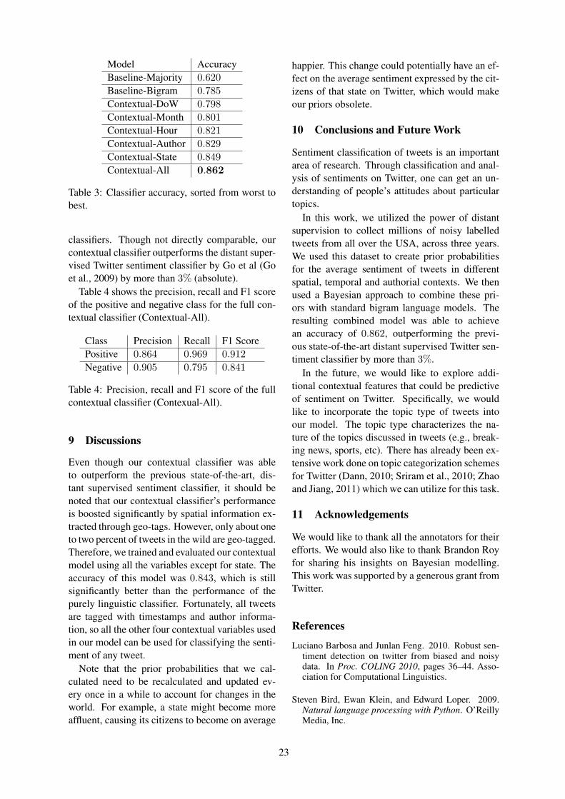
Model AccuracyBaseline-Majority 0.620Baseline-Bigram 0.785Contextual-DoW 0.798Contextual-Month 0.801Contextual-Hour 0.821Contextual-Author 0.829Contextual-State 0.849Contextual-All 0.862

Table 3: Classifier accuracy, sorted from worst tobest.

classifiers. Though not directly comparable, ourcontextual classifier outperforms the distant super-vised Twitter sentiment classifier by Go et al (Goet al., 2009) by more than 3% (absolute).

Table 4 shows the precision, recall and F1 scoreof the positive and negative class for the full con-textual classifier (Contextual-All).

Class Precision Recall F1 ScorePositive 0.864 0.969 0.912Negative 0.905 0.795 0.841

Table 4: Precision, recall and F1 score of the fullcontextual classifier (Contexual-All).

9 Discussions

Even though our contextual classifier was ableto outperform the previous state-of-the-art, dis-tant supervised sentiment classifier, it should benoted that our contextual classifier’s performanceis boosted significantly by spatial information ex-tracted through geo-tags. However, only about oneto two percent of tweets in the wild are geo-tagged.Therefore, we trained and evaluated our contextualmodel using all the variables except for state. Theaccuracy of this model was 0.843, which is stillsignificantly better than the performance of thepurely linguistic classifier. Fortunately, all tweetsare tagged with timestamps and author informa-tion, so all the other four contextual variables usedin our model can be used for classifying the senti-ment of any tweet.

Note that the prior probabilities that we cal-culated need to be recalculated and updated ev-ery once in a while to account for changes in theworld. For example, a state might become moreaffluent, causing its citizens to become on average

happier. This change could potentially have an ef-fect on the average sentiment expressed by the cit-izens of that state on Twitter, which would makeour priors obsolete.

10 Conclusions and Future Work

Sentiment classification of tweets is an importantarea of research. Through classification and anal-ysis of sentiments on Twitter, one can get an un-derstanding of people’s attitudes about particulartopics.

In this work, we utilized the power of distantsupervision to collect millions of noisy labelledtweets from all over the USA, across three years.We used this dataset to create prior probabilitiesfor the average sentiment of tweets in differentspatial, temporal and authorial contexts. We thenused a Bayesian approach to combine these pri-ors with standard bigram language models. Theresulting combined model was able to achievean accuracy of 0.862, outperforming the previ-ous state-of-the-art distant supervised Twitter sen-timent classifier by more than 3%.

In the future, we would like to explore addi-tional contextual features that could be predictiveof sentiment on Twitter. Specifically, we wouldlike to incorporate the topic type of tweets intoour model. The topic type characterizes the na-ture of the topics discussed in tweets (e.g., break-ing news, sports, etc). There has already been ex-tensive work done on topic categorization schemesfor Twitter (Dann, 2010; Sriram et al., 2010; Zhaoand Jiang, 2011) which we can utilize for this task.

11 Acknowledgements

We would like to thank all the annotators for theirefforts. We would also like to thank Brandon Royfor sharing his insights on Bayesian modelling.This work was supported by a generous grant fromTwitter.

References

Luciano Barbosa and Junlan Feng. 2010. Robust sen-timent detection on twitter from biased and noisydata. In Proc. COLING 2010, pages 36–44. Asso-ciation for Computational Linguistics.

Steven Bird, Ewan Klein, and Edward Loper. 2009.Natural language processing with Python. O’ReillyMedia, Inc.

23

Johan Bollen, Huina Mao, and Alberto Pepe. 2011.Modeling public mood and emotion: Twitter sen-timent and socio-economic phenomena. In Proc.ICWSM 2011.

Stanley F Chen and Joshua Goodman. 1999. Anempirical study of smoothing techniques for lan-guage modeling. Computer Speech & Language,13(4):359–393.

Paula Chesley, Bruce Vincent, Li Xu, and Rohini KSrihari. 2006. Using verbs and adjectives toautomatically classify blog sentiment. Training,580(263):233.

Mihaly Csikszentmihalyi and Jeremy Hunter. 2003.Happiness in everyday life: The uses of experiencesampling. Journal of Happiness Studies, 4(2):185–199.

Hang Cui, Vibhu Mittal, and Mayur Datar. 2006.Comparative experiments on sentiment classifica-tion for online product reviews. In AAAI, volume 6,pages 1265–1270.

Stephen Dann. 2010. Twitter content classification.First Monday, 15(12).

Dmitry Davidov, Oren Tsur, and Ari Rappoport. 2010.Enhanced sentiment learning using twitter hashtagsand smileys. In Proc. COLING 2010, pages 241–249. Association for Computational Linguistics.

Nicholas A Diakopoulos and David A Shamma. 2010.Characterizing debate performance via aggregatedtwitter sentiment. In Proc. SIGCHI 2010, pages1195–1198. ACM.

Joseph L Fleiss. 1971. Measuring nominal scaleagreement among many raters. Psychological bul-letin, 76(5):378.

Gallup-Healthways. 2014. State of american well-being. Well-Being Index.

Alec Go, Lei Huang, and Richa Bhayani. 2009. Twit-ter sentiment analysis. Entropy, 17.

Long Jiang, Mo Yu, Ming Zhou, Xiaohua Liu, andTiejun Zhao. 2011. Target-dependent twitter sen-timent classification. In Proc. ACL 2011: HumanLanguage Technologies-Volume 1, pages 151–160.Association for Computational Linguistics.

Slava Katz. 1987. Estimation of probabilities fromsparse data for the language model component ofa speech recognizer. Acoustics, Speech and SignalProcessing, IEEE Transactions on, 35(3):400–401.

Efthymios Kouloumpis, Theresa Wilson, and JohannaMoore. 2011. Twitter sentiment analysis: The goodthe bad and the omg! Proc. ICWSM 2011.

Lewis Mitchell, Morgan R Frank, Kameron DeckerHarris, Peter Sheridan Dodds, and Christopher MDanforth. 2013. The geography of happiness:

Connecting twitter sentiment and expression, de-mographics, and objective characteristics of place.PloS one, 8(5):e64417.

Robert J Moore. 2009. Twitter dataanalysis: An investor’s perspective.http://techcrunch.com/2009/10/05/twitter-data-analysis-an-investors-perspective-2/. Accessed:2015-01-30.

Tetsuji Nakagawa, Kentaro Inui, and Sadao Kurohashi.2010. Dependency tree-based sentiment classifi-cation using crfs with hidden variables. In Proc.NAACL-HLT 2010, pages 786–794. Association forComputational Linguistics.

Andrew J Oswald and Stephen Wu. 2011. Well-beingacross america. Review of Economics and Statistics,93(4):1118–1134.

Bo Pang, Lillian Lee, and Shivakumar Vaithyanathan.2002. Thumbs up?: sentiment classification us-ing machine learning techniques. In Proc. EMNLP2002-Volume 10, pages 79–86. Association forComputational Linguistics.

Martin F Porter. 1980. An algorithm for suffix strip-ping. Program: electronic library and informationsystems, 14(3):130–137.

Jonathon Read. 2005. Using emoticons to reduce de-pendency in machine learning techniques for senti-ment classification. In Proceedings of the ACL Stu-dent Research Workshop, pages 43–48. Associationfor Computational Linguistics.

Hassan Saif, Yulan He, and Harith Alani. 2012. Al-leviating data sparsity for twitter sentiment analysis.CEUR Workshop Proceedings (CEUR-WS. org).

Bharath Sriram, Dave Fuhry, Engin Demir, Hakan Fer-hatosmanoglu, and Murat Demirbas. 2010. Shorttext classification in twitter to improve informationfiltering. In Proc. ACM SIGIR 2010, pages 841–842.ACM.

Xiaolong Wang, Furu Wei, Xiaohua Liu, Ming Zhou,and Ming Zhang. 2011. Topic sentiment analysisin twitter: a graph-based hashtag sentiment classifi-cation approach. In Proc. CIKM 2011, pages 1031–1040. ACM.

Xin Zhao and Jing Jiang. 2011. An empirical compari-son of topics in twitter and traditional media. Singa-pore Management University School of InformationSystems Technical paper series. Retrieved Novem-ber, 10:2011.

24