Embed Size (px)
Citation preview
APPENDIX 6
EPANET – Version 2(based on the EPANET 2 Users Manual by L.A. Rossman1)
A6.1 INSTALLATION
EPANET 2 is a computer programme that performs hydraulic and waterquality simulations of drinking water distribution systems. For a basic setof input data related to the geometry of the network and the waterdemand levels in it, the programme is able to determine the flow of waterin each pipe, the pressure at each pipe junction, the flows and heads ateach pump, and the water depth in each storage tank. Additional infor-mation on water quality parameters serves to calculate the concentrationof a substance throughout a distribution system. In addition to substanceconcentrations, water age and source tracing can also be simulated. Theuser is able to edit EPANET 2 files and, after running a simulation, dis-play the results on a colour-coded map of the distribution system andgenerate additional tabular and graphical views of these results.
The calculations made by EPANET can help in solving all sorts ofpractical problems, such as:– the design of new extensions and pumping stations,– the analysis of pumps’ energy and cost,– the optimal operation which can guarantee delivery of sufficient water
quality and pressure,– the assessment of network reliability,– the development of effective flushing programmes,– the use of satellite treatment, such as re-chlorination at storage tanks,– the diagnosis of water quality problems, etc.
EPANET 2 software (EN2setup.exe) and its manual (EN2manual.pdf)are in the public domain and can be downloaded from the website ofthe US Environmental Protection Agency. This site is easily accessiblethrough any search engine (e.g. ‘Google’), by using the keyword‘epanet’.
1 Rossman, L.A., EPANET 2 Users Manual, EPA/600/R-00/57, Water Supply and Water Resources Division, U.S.Environmental Protection Agency, Cincinnati, OH, September 2000).
EPANET Instructions for Use 473
The file EN2setup.exe contains a self-extracting setup programme.The installation starts after double-clicking on this file. The defaultprogramme directory is c:\Program Files\EPANET2, which can bechanged during the process that will be fully completed in just a fewseconds. After the programme has been installed, the Start Menu willhave a new item named EPANET 2.0. To start the programme, chooseStart Programs Epanet 2.0 Epanet 2.0.
A6.2 USING THE PROGRAMME
After running the programme, a screen with the menu bar, toolbars,blank network map window and the browser window will appear.
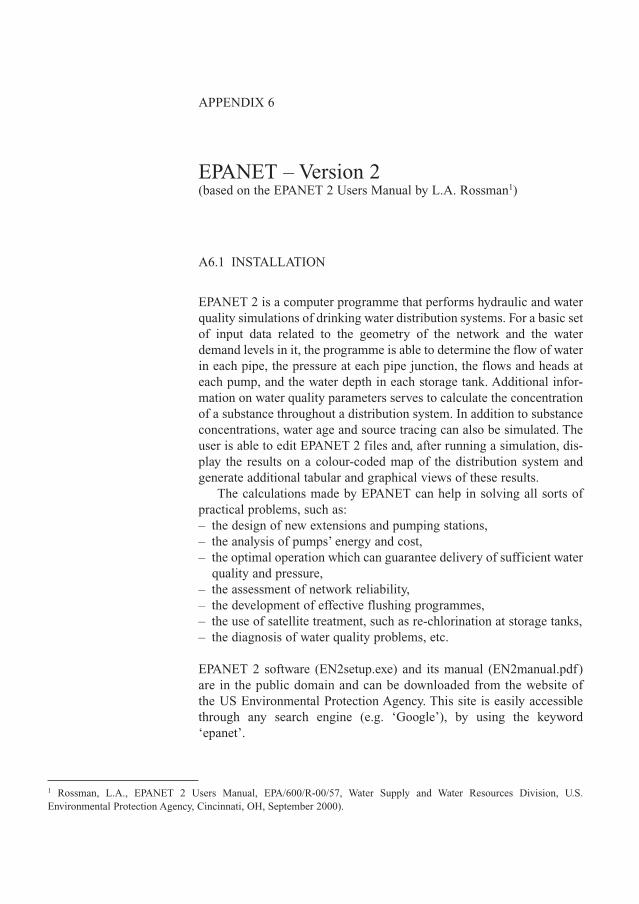
Menu bar The Menu bar located across the top of the EPANET workspace containsa collection of menus used to control the program. These include:
File Menu
Edit Menu
Creates a new project
Opens an existing project
Saves the current project
Imports network data or map from a file
Exports network data or map to a file
Sets page margins, headers and footers for printing
Exits EPANET
Saves the current project under a different name
Previews a printout of the current view
Prints the current view
Sets the general preferences
Copies the currently active view (map, report, graph or table)to the clipboard or to a file
Allows selection of an object on the map
Allows selection of link vertices on the map
Allows selection of an outlined region on the map
Makes the outlined region the entire viewable map area
Edits a property for the group of objects that fall within theoutlined region of the map
474 Introduction to Urban Water Distribution
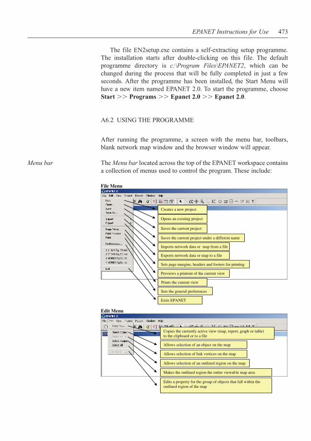
View Menu
Project Menu
Dimensions of the map
Allows a backdrop map to be viewed
Pans across the map
Zooms in on the map
Zooms out on the map
Redraws the map at full extent
Locates a specific item on the map
Searches for items on the map that meet specific criteria
Toggles the overview Map on/off
Controls the display of map legends
Toggles the toolbars on/off
Sets map appearance options
Provides a summary description of the project's characteristics
Edits a project's default properties
Registers files containing calibration data with the project
Edits analysis options
Runs a simulation
Report Menu
Reports changes in the status of links over time
Reports the energy consumed by each pump
Reports differences between simulated and measured values
Reports average reaction rates throughout the network
Creates the full report of computed results for all nodes andlinks in all time periods which is saved to a plain text file
Creates various diagrams or maps of computed results: for selected nodes, links, any parameter or the entire system flow
Creates a tabular display of selected node and link quantities
Controls the display style of a report, graph, or table
EPANET Instructions for Use 475
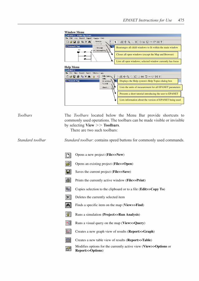
Window Menu
Help Menu
Rearranges all child windows to fit within the main window
Closes all open windows (except the Map and Browser)
Lists all open windows; selected window currently has focus
Displays the Help system's Help Topics dialog box
Lists the units of measurement for all EPANET parameters
Presents a short tutorial introducing the user to EPANET
Lists information about the version of EPANET being used
Opens a new project (File>>New)
Opens an existing project (File>>Open)
Saves the current project (File>>Save)
Prints the currently active window (File>>Print)
Copies selection to the clipboard or to a file (Edit>>Copy To)
Deletes the currently selected item
Finds a specific item on the map (View>>Find)
Runs a simulation (Project>>Run Analysis)
Runs a visual query on the map (View>>Query)
Creates a new graph view of results (Report>>Graph)
Creates a new table view of results (Report>>Table)
Modifies options for the currently active view (View>>Options orReport>>Options)
Toolbars The Toolbars located below the Menu Bar provide shortcuts tocommonly used operations. The toolbars can be made visible or invisibleby selecting View Toolbars.
There are two such toolbars:
Standard toolbar Standard toolbar: contains speed buttons for commonly used commands.
476 Introduction to Urban Water Distribution
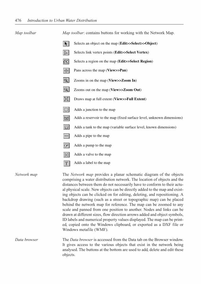
Map toolbar Map toolbar: contains buttons for working with the Network Map.
Selects an object on the map (Edit>>Select>>Object)
Selects link vertex points (Edit>>Select Vertex)
Selects a region on the map (Edit>>Select Region)
Pans across the map (View>>Pan)
Zooms in on the map (View>>Zoom In)
Zooms out on the map (View>>Zoom Out)
Draws map at full extent (View>>Full Extent)
Adds a junction to the map
Adds a reservoir to the map (fixed surface level, unknown dimensions)
Adds a tank to the map (variable surface level, known dimensions)
Adds a pipe to the map
Adds a pump to the map
Adds a valve to the map
Adds a label to the map
Network map The Network map provides a planar schematic diagram of the objectscomprising a water distribution network. The location of objects and thedistances between them do not necessarily have to conform to their actu-al physical scale. New objects can be directly added to the map and exist-ing objects can be clicked on for editing, deleting, and repositioning. Abackdrop drawing (such as a street or topographic map) can be placedbehind the network map for reference. The map can be zoomed to anyscale and panned from one position to another. Nodes and links can bedrawn at different sizes, flow direction arrows added and object symbols,ID labels and numerical property values displayed. The map can be print-ed, copied onto the Windows clipboard, or exported as a DXF file orWindows metafile (WMF).
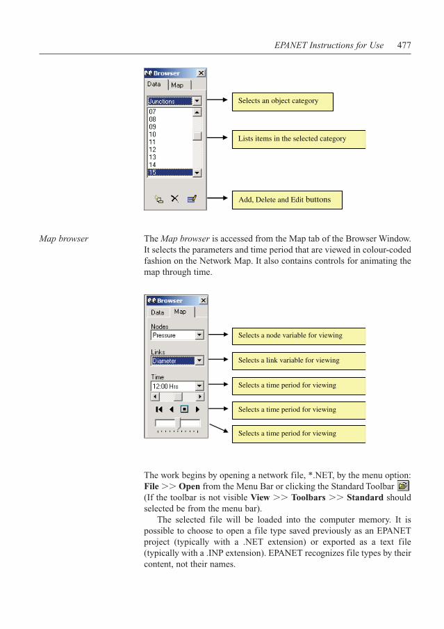
Data browser The Data browser is accessed from the Data tab on the Browser window.It gives access to the various objects that exist in the network beinganalysed. The buttons at the bottom are used to add, delete and edit theseobjects.
EPANET Instructions for Use 477
Map browser The Map browser is accessed from the Map tab of the Browser Window.It selects the parameters and time period that are viewed in colour-codedfashion on the Network Map. It also contains controls for animating themap through time.
The work begins by opening a network file, *.NET, by the menu option:File Open from the Menu Bar or clicking the Standard Toolbar(If the toolbar is not visible View Toolbars Standard shouldselected be from the menu bar).
The selected file will be loaded into the computer memory. It ispossible to choose to open a file type saved previously as an EPANETproject (typically with a .NET extension) or exported as a text file(typically with a .INP extension). EPANET recognizes file types by theircontent, not their names.
Selects an object category
Lists items in the selected category
Add, Delete and Edit buttons
Selects a node variable for viewing
Selects a link variable for viewing
Selects a time period for viewing
Selects a time period for viewing
Selects a time period for viewing
478 Introduction to Urban Water Distribution
Calculation starts by running the menu option: Project RunAnalysis or clicking the Run button on the Standard Toolbar.
Status report If the run was unsuccessful then a Status report window will appearindicating what the problem was. In some situations, the calculation maybe completed regardless of the hydraulic boundary conditions. A warn-ing message is displayed in that case. The input data have to be careful-ly analysed. More information about the calculation progress can berequested in repeated trials. The details about this, together with thedescription of other programme features, are presented in the full versionof the programme manual.
If it ran successfully, the user can view the computed results in avariety of ways:
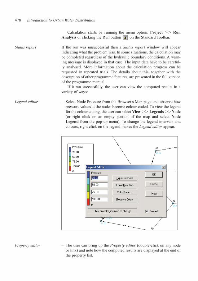
Legend editor – Select Node Pressure from the Browser’s Map page and observe howpressure values at the nodes become colour-coded. To view the legendfor the colour coding, the user can select View Legends Node(or right click on an empty portion of the map and select NodeLegend from the pop-up menu). To change the legend intervals andcolours, right click on the legend makes the Legend editor appear.
Property editor – The user can bring up the Property editor (double-click on any nodeor link) and note how the computed results are displayed at the end ofthe property list.
EPANET Instructions for Use 479
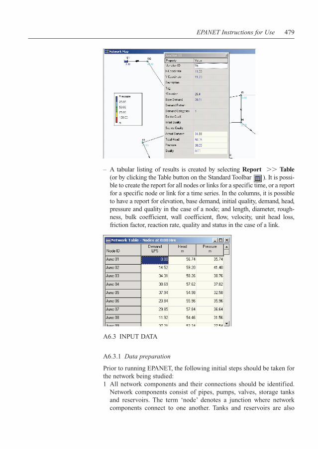
– A tabular listing of results is created by selecting Report Table(or by clicking the Table button on the Standard Toolbar ). It is possi-ble to create the report for all nodes or links for a specific time, or a reportfor a specific node or link for a time series. In the columns, it is possibleto have a report for elevation, base demand, initial quality, demand, head,pressure and quality in the case of a node; and length, diameter, rough-ness, bulk coefficient, wall coefficient, flow, velocity, unit head loss,friction factor, reaction rate, quality and status in the case of a link.
A6.3 INPUT DATA
A6.3.1 Data preparation
Prior to running EPANET, the following initial steps should be taken forthe network being studied:1 All network components and their connections should be identified.
Network components consist of pipes, pumps, valves, storage tanksand reservoirs. The term ‘node’ denotes a junction where networkcomponents connect to one another. Tanks and reservoirs are also

considered as nodes. The component (pipe, pump or valve) connectingany two nodes is termed a ‘link’.
2 Unique ID numbers should be assigned to all nodes. ID numbers mustbe between 1 and 2,147,483,647, but need not to be in any specificorder nor be consecutive.
3 An ID number should be assigned to each link (pipe, pump or valve). Itis permissible to use the same ID number for both a node and a link.
4 The following information should be collected on the system parameters:a diameter, length, roughness and minor loss coefficient for each pipe,b the characteristic operating curve for each pump,c diameter, minor loss coefficient and pressure or flow setting for
each control valve,d diameter and minimum and maximum water depths for each tank,e control rules that determine how pump, valve and pipe settings
change with time, tank water levels or nodal pressures,f changes in water demands for each node over the time period being
simulated,g initial water quality at all nodes and changes in water quality over
time at source nodes.
With this information at hand, it is now possible to construct an input fileto use with EPANET.
A6.3.2 Selecting objects
To select an object on the map:
Selection mode – The map must be in Selection mode (the mouse cursor has the shapeof an arrow pointing up to the left). To switch to this mode, the usershould either click the Select Object button on the Map Toolbaror choose Edit Select Object from the menu bar.
– The mouse has to be clicked over the desired object on the map.
To select an object using the Browser:– The category of object has to be seleceted from the dropdown list of
the Data Browser.– The desired object has to be selected from the list below the category
heading.
A6.3.3 Editing visual objects
The Property Editor is used to edit the properties of objects that can appearon the Network Map (Junctions, Reservoirs, Tanks, Pipes, Pumps, Valves orLabels). To edit one of these objects, the user should select the object on themap or from the Data Browser, then click the Edit button on the DataBrowser (or simply double-click the object on the map). The propertiesassociated with each of these types of objects are described in Tables 1 to 7.
480 Introduction to Urban Water Distribution
EPANET Instructions for Use 481
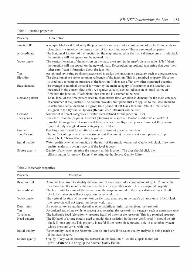
Table 1 Junction properties
Property Description
Junction ID A unique label used to identify the junction. It can consist of a combination of up to 15 numerals or characters. It cannot be the same as the ID for any other node. This is a required property.
X-coordinate The horizontal location of the junction on the map, measured in the map’s distance units. If left blank the junction will not appear on the network map.
Y-coordinate The vertical location of the junction on the map, measured in the map’s distance units. If left blank the junction will not appear on the network map. Description: an optional text string that describes other significant information about the junction.
Tag An optional text string (with no spaces) used to assign the junction to a category, such as a pressure zone.Elevation The elevation above some common reference of the junction. This is a required property. Elevation
is used only to compute pressure at the junction. It does not affect any other computed quantity.Base demand The average or nominal demand for water by the main category of consumer at the junction, as
measured in the current flow units. A negative value is used to indicate an external source of flow into the junction. If left blank then demand is assumed to be zero.
Demand pattern The ID label of the time pattern used to characterize time variation in demand for the main category of consumer at the junction. The pattern provides multipliers that are applied to the Base Demand to determine actual demand in a given time period. If left blank then the Default Time Pattern assigned in the Hydraulic Options (Report Default) will be used.
Demand Number of different categories of water users defined for the junction. Clickcategories the ellipsis button (or press �Enter) to bring up a special Demands Editor which makes it
possible to assign base demands and time patterns to multiple categories of users at the junction. Ignore if only a single demand category will suffice.
Emitter Discharge coefficient for emitter (sprinkler or nozzle) placed at junction.coefficient The coefficient represents the flow (in current flow units) that occurs at a unit pressure drop. It
should be left blank if no emitter is present.Initial quality Water quality level at the junction at the start of the simulation period. Can be left blank if no water
quality analysis is being made or if the level is zero.Source quality Quality of any water entering the network at this location. The user should click the
ellipsis button (or press �Enter) to bring up the Source Quality Editor.
Table 2 Reservoir properties
Property Description
Reservoir ID A unique label used to identify the reservoir. It can consist of a combination of up to 15 numerals or characters. It cannot be the same as the ID for any other node. This is a required property.
X-coordinate The horizontal location of the reservoir on the map, measured in the map’s distance units. If left blank the reservoir will not appear on the network map.
Y-coordinate The vertical location of the reservoir on the map, measured in the map’s distance units. If left blank the reservoir will not appear on the network map.
Description An optional text string that describes other significant information about the reservoir.Tag An optional text string (with no spaces) used to assign the reservoir to a category, such as a pressure zoneTotal head The hydraulic head (elevation � pressure head) of water in the reservoir. This is a required property.Head pattern The ID label of a time pattern used to model time variation in the reservoir’s head. It should be left
blank if none applies. This property is useful if the reservoir represents a tie-in to another system whose pressure varies with time.
Initial quality Water quality level at the reservoir. Can be left blank if no water quality analysis is being made or if the level is zero.
Source quality Quality of any water entering the network at this location. Click the ellipsis button (orpress �Enter) to bring up the Source Quality Editor.
482 Introduction to Urban Water Distribution
Table 3 Tank properties
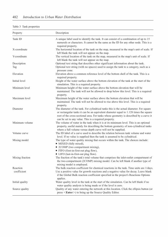
Property Description
Tank ID A unique label used to identify the tank. It can consist of a combination of up to 15numerals or characters. It cannot be the same as the ID for any other node. This is arequired property.
X-coordinate The horizontal location of the tank on the map, measured in the map’s unit of scale. Ifleft blank the tank will not appear on the map.
Y-coordinate The vertical location of the tank on the map, measured in the map’s unit of scale. Ifleft blank the tank will not appear on the map.
Description Optional text string that describes other significant information about the tank.Tag Optional text string (with no spaces) used to assign the tank to a category, such as a
pressure zone.Elevation Elevation above a common reference level of the bottom shell of the tank. This is a
required property.Initial level Height of the water surface above the bottom elevation of the tank at the start of the
simulation. This is a required property.Minimum level Minimum height of the water surface above the bottom elevation that will be
maintained. The tank will not be allowed to drop below this level. This is a requiredproperty.
Maximum level Maximum height of the water surface above the bottom elevation that will bemaintained. The tank will not be allowed to rise above this level. This is a requiredproperty.
Diameter The diameter of the tank. For cylindrical tanks this is the actual diameter. For squareor rectangular tanks it can be an equivalent diameter equal to 1.128 times the squareroot of the cross-sectional area. For tanks whose geometry is described by a curve itcan be set to any value. This is a required property.
Minimum volume The volume of water in the tank when it is at its minimum level. This is an optionalproperty, useful mainly for describing the bottom geometry of non-cylindrical tankswhere a full volume versus depth curve will not be supplied.
Volume curve The ID label of a curve used to describe the relation between tank volume and waterlevel. If no value is supplied then the tank is assumed to be cylindrical.
Mixing model The type of water quality mixing that occurs within the tank. The choices include:● MIXED (fully mixed),● 2COMP (two compartment mixing),● FIFO (first-in-first-out plug flow),● LIFO (last-in-first-out plug flow).
Mixing fraction The fraction of the tank’s total volume that comprises the inlet-outlet compartment ofthe two-compartment (2COMP) mixing model. Can be left blank if another type ofmixing model is employed.
Reaction The bulk reaction coefficient for chemical reactions in the tank. Time units are 1/days.coefficient Use a positive value for growth reactions and a negative value for decay. Leave blank
if the Global Bulk reaction coefficient specified in the project’s Reactions Optionsapplies.
Initial quality Water quality level in the tank at the start of the simulation. Can be left blank if nowater quality analysis is being made or if the level is zero.
Source quality Quality of any water entering the network at this location. Click the ellipsis button (orpress �Enter) to bring up the Source Quality Editor.
EPANET Instructions for Use 483
Table 4 Pipe properties
Property Description
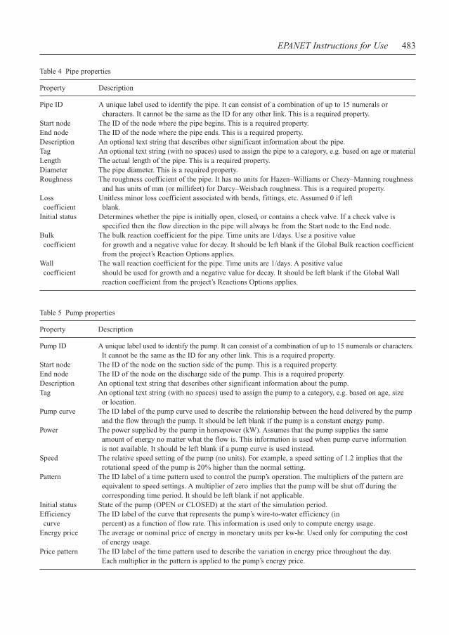
Pipe ID A unique label used to identify the pipe. It can consist of a combination of up to 15 numerals or characters. It cannot be the same as the ID for any other link. This is a required property.
Start node The ID of the node where the pipe begins. This is a required property.End node The ID of the node where the pipe ends. This is a required property.Description An optional text string that describes other significant information about the pipe.Tag An optional text string (with no spaces) used to assign the pipe to a category, e.g. based on age or materialLength The actual length of the pipe. This is a required property.Diameter The pipe diameter. This is a required property.Roughness The roughness coefficient of the pipe. It has no units for Hazen–Williams or Chezy–Manning roughness
and has units of mm (or millifeet) for Darcy–Weisbach roughness. This is a required property.Loss Unitless minor loss coefficient associated with bends, fittings, etc. Assumed 0 if leftcoefficient blank.
Initial status Determines whether the pipe is initially open, closed, or contains a check valve. If a check valve is specified then the flow direction in the pipe will always be from the Start node to the End node.
Bulk The bulk reaction coefficient for the pipe. Time units are 1/days. Use a positive valuecoefficient for growth and a negative value for decay. It should be left blank if the Global Bulk reaction coefficient
from the project’s Reaction Options applies.Wall The wall reaction coefficient for the pipe. Time units are 1/days. A positive valuecoefficient should be used for growth and a negative value for decay. It should be left blank if the Global Wall
reaction coefficient from the project’s Reactions Options applies.
Table 5 Pump properties
Property Description
Pump ID A unique label used to identify the pump. It can consist of a combination of up to 15 numerals or characters. It cannot be the same as the ID for any other link. This is a required property.
Start node The ID of the node on the suction side of the pump. This is a required property.End node The ID of the node on the discharge side of the pump. This is a required property.Description An optional text string that describes other significant information about the pump.Tag An optional text string (with no spaces) used to assign the pump to a category, e.g. based on age, size
or location.Pump curve The ID label of the pump curve used to describe the relationship between the head delivered by the pump
and the flow through the pump. It should be left blank if the pump is a constant energy pump.Power The power supplied by the pump in horsepower (kW). Assumes that the pump supplies the same
amount of energy no matter what the flow is. This information is used when pump curve information is not available. It should be left blank if a pump curve is used instead.
Speed The relative speed setting of the pump (no units). For example, a speed setting of 1.2 implies that the rotational speed of the pump is 20% higher than the normal setting.
Pattern The ID label of a time pattern used to control the pump’s operation. The multipliers of the pattern are equivalent to speed settings. A multiplier of zero implies that the pump will be shut off during the corresponding time period. It should be left blank if not applicable.
Initial status State of the pump (OPEN or CLOSED) at the start of the simulation period.Efficiency The ID label of the curve that represents the pump’s wire-to-water efficiency (incurve percent) as a function of flow rate. This information is used only to compute energy usage.
Energy price The average or nominal price of energy in monetary units per kw-hr. Used only for computing the cost of energy usage.
Price pattern The ID label of the time pattern used to describe the variation in energy price throughout the day. Each multiplier in the pattern is applied to the pump’s energy price.
484 Introduction to Urban Water Distribution
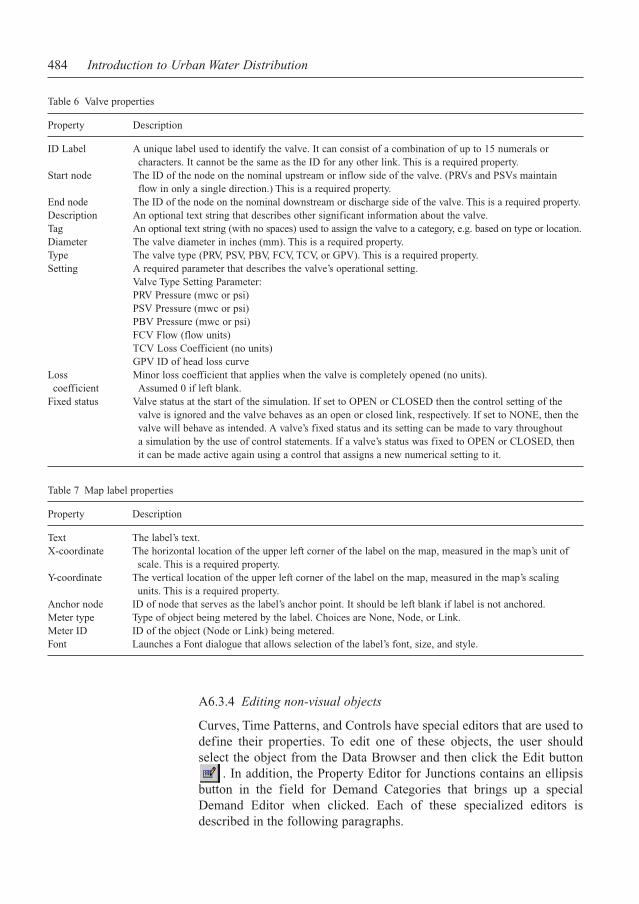
Table 6 Valve properties
Property Description
ID Label A unique label used to identify the valve. It can consist of a combination of up to 15 numerals or characters. It cannot be the same as the ID for any other link. This is a required property.
Start node The ID of the node on the nominal upstream or inflow side of the valve. (PRVs and PSVs maintain flow in only a single direction.) This is a required property.
End node The ID of the node on the nominal downstream or discharge side of the valve. This is a required property.Description An optional text string that describes other significant information about the valve.Tag An optional text string (with no spaces) used to assign the valve to a category, e.g. based on type or location.Diameter The valve diameter in inches (mm). This is a required property.Type The valve type (PRV, PSV, PBV, FCV, TCV, or GPV). This is a required property.Setting A required parameter that describes the valve’s operational setting.
Valve Type Setting Parameter:PRV Pressure (mwc or psi)PSV Pressure (mwc or psi)PBV Pressure (mwc or psi)FCV Flow (flow units)TCV Loss Coefficient (no units)GPV ID of head loss curve
Loss Minor loss coefficient that applies when the valve is completely opened (no units).coefficient Assumed 0 if left blank.
Fixed status Valve status at the start of the simulation. If set to OPEN or CLOSED then the control setting of the valve is ignored and the valve behaves as an open or closed link, respectively. If set to NONE, then the valve will behave as intended. A valve’s fixed status and its setting can be made to vary throughout a simulation by the use of control statements. If a valve’s status was fixed to OPEN or CLOSED, then it can be made active again using a control that assigns a new numerical setting to it.
Table 7 Map label properties
Property Description
Text The label’s text.X-coordinate The horizontal location of the upper left corner of the label on the map, measured in the map’s unit of
scale. This is a required property.Y-coordinate The vertical location of the upper left corner of the label on the map, measured in the map’s scaling
units. This is a required property.Anchor node ID of node that serves as the label’s anchor point. It should be left blank if label is not anchored.Meter type Type of object being metered by the label. Choices are None, Node, or Link.Meter ID ID of the object (Node or Link) being metered.Font Launches a Font dialogue that allows selection of the label’s font, size, and style.
A6.3.4 Editing non-visual objects
Curves, Time Patterns, and Controls have special editors that are used todefine their properties. To edit one of these objects, the user shouldselect the object from the Data Browser and then click the Edit button
. In addition, the Property Editor for Junctions contains an ellipsisbutton in the field for Demand Categories that brings up a specialDemand Editor when clicked. Each of these specialized editors isdescribed in the following paragraphs.
EPANET Instructions for Use 485
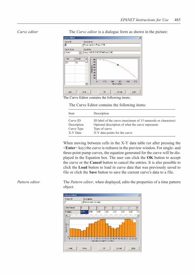
The Curve Editor contains the following items:
Item Description
Curve ID ID label of the curve (maximum of 15 numerals or characters)Description Optional description of what the curve representsCurve Type Type of curveX-Y Data X-Y data points for the curve
When moving between cells in the X-Y data table (or after pressing the<Enter> key) the curve is redrawn in the preview window. For single- andthree-point pump curves, the equation generated for the curve will be dis-played in the Equation box. The user can click the OK button to acceptthe curve or the Cancel button to cancel the entries. It is also possible toclick the Load button to load in curve data that was previously saved tofile or click the Save button to save the current curve’s data to a file.
Pattern editor The Pattern editor, when displayed, edits the properties of a time patternobject.
Curve editor The Curve editor is a dialogue form as shown in the picture:
The Curve Editor contains the following items:
486 Introduction to Urban Water Distribution
To use the Pattern editor values for the following items should be entered:
Item Description
Pattern ID ID label of the pattern (maximum of 15 numerals or characters).Description Optional description of what the pattern represents.Multipliers Multiplier value for each time period of the pattern.
Time periods As multipliers are entered, the preview chart is redrawn to provide a visu-al depiction of the pattern. If the end of the available Time periods isreached when entering multipliers, pressing �Enter adds on anotherperiod. When finished editing, clicking OK accepts the pattern whilstthe Cancel button cancels the entries. It is also possible to click Load toload in pattern data that was previously saved to file or click Save to savethe current pattern’s data to a file.
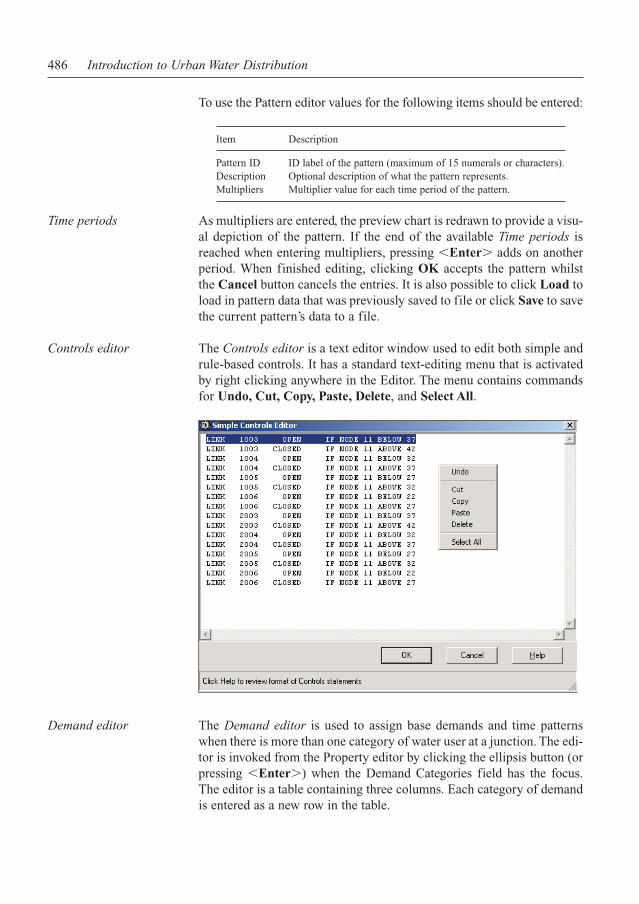
Controls editor The Controls editor is a text editor window used to edit both simple andrule-based controls. It has a standard text-editing menu that is activatedby right clicking anywhere in the Editor. The menu contains commandsfor Undo, Cut, Copy, Paste, Delete, and Select All.
Demand editor The Demand editor is used to assign base demands and time patternswhen there is more than one category of water user at a junction. The edi-tor is invoked from the Property editor by clicking the ellipsis button (orpressing �Enter) when the Demand Categories field has the focus.The editor is a table containing three columns. Each category of demandis entered as a new row in the table.
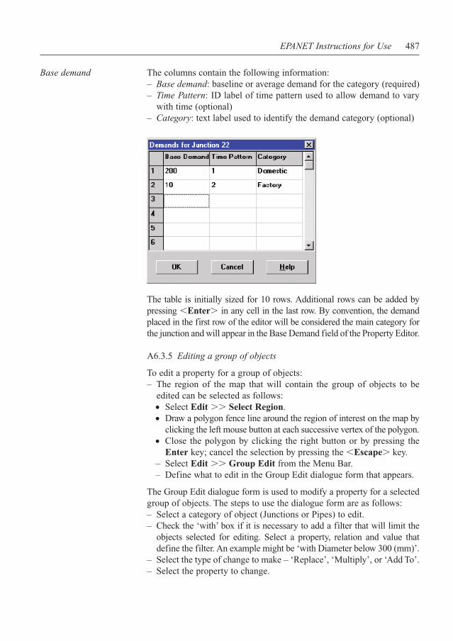
EPANET Instructions for Use 487
Base demand The columns contain the following information:– Base demand: baseline or average demand for the category (required)– Time Pattern: ID label of time pattern used to allow demand to vary
with time (optional)– Category: text label used to identify the demand category (optional)
The table is initially sized for 10 rows. Additional rows can be added bypressing �Enter in any cell in the last row. By convention, the demandplaced in the first row of the editor will be considered the main category forthe junction and will appear in the Base Demand field of the Property Editor.
A6.3.5 Editing a group of objects
To edit a property for a group of objects:– The region of the map that will contain the group of objects to be
edited can be selected as follows:● Select Edit Select Region.● Draw a polygon fence line around the region of interest on the map by
clicking the left mouse button at each successive vertex of the polygon.● Close the polygon by clicking the right button or by pressing the
Enter key; cancel the selection by pressing the �Escape key.– Select Edit Group Edit from the Menu Bar.– Define what to edit in the Group Edit dialogue form that appears.
The Group Edit dialogue form is used to modify a property for a selectedgroup of objects. The steps to use the dialogue form are as follows:– Select a category of object (Junctions or Pipes) to edit.– Check the ‘with’ box if it is necessary to add a filter that will limit the
objects selected for editing. Select a property, relation and value thatdefine the filter. An example might be ‘with Diameter below 300 (mm)’.
– Select the type of change to make – ‘Replace’, ‘Multiply’, or ‘Add To’.– Select the property to change.

488 Introduction to Urban Water Distribution
– Enter the value that should replace, multiply, or be added to theexisting value.
– Click OK to execute the group edit.
A6.4 VIEWING RESULTS
A6.4.1 Viewing results on the map
There are several ways in which database values and results of a simula-tion can be viewed directly on the Network Map:
● For the current settings on the Map Browser the nodes and links ofthe map will be coloured according to the colour coding used in theMap Legends. The map’s colouring will be updated as a new timeperiod is selected in the Browser.
● ID labels and viewing parameter values can be displayed next to allnodes and/or links by selecting the appropriate options on theNotation page of the Map Options dialogue form.
● The display of results on the network map can be animated eitherforward or backward in time by using the Animation buttons on theMap Browser. Animation is only available when a node or linkviewing parameter is a computed value (e.g. link flow rate can beanimated but diameter cannot).
● The map can be printed, copied to the Windows clipboard, or savedas a DXF or WMF file.
● Nodes or links meeting a specific criterion can be identified bysubmitting a Map query; the user should execute the following steps:
Select whether to search for Nodes or Links
Select a parameter to compare against
Select ‘Above’, ‘Below’, or ‘Equals’
Enter a value to compare against
EPANET Instructions for Use 489
Map query 1 Select a time period in which to query the map from the Map Browser.
2 Select View Query or click on the Map Toolbar.3 Fill in the following information in the Query dialogue form that
appears.4 Click the Submit button. The objects that meet the criterion will be
highlighted on the map.5 As a new time period is selected in the Browser, the query results are
automatically updated.6 It is possible to submit another query using the dialogue box or close
it by clicking the button in the upper right corner.
A6.4.2 Viewing results with a graph
Analysis results, as well as some design parameters, can be viewedusing several different types of graphs. Graphs can be printed, copied tothe Windows clipboard, or saved as a data file or Windows metafile. Thefollowing types of graphs can be used to view values for a selectedparameter:
Type of plot Description Applies to
Time Series plot Plots value versus time Specific nodes or links over all timeperiods
Profile plot Plots value versus distance A list of nodes at a specific timeContour plot Shows regions of the All nodes at a specific time
map where values fall within specific intervals
Frequency plot Plots value versus fraction of All nodes or links at a objects at or below the value specific time
System flow Plots total system production Water demand for all nodes and consumption versus over all time periodstime
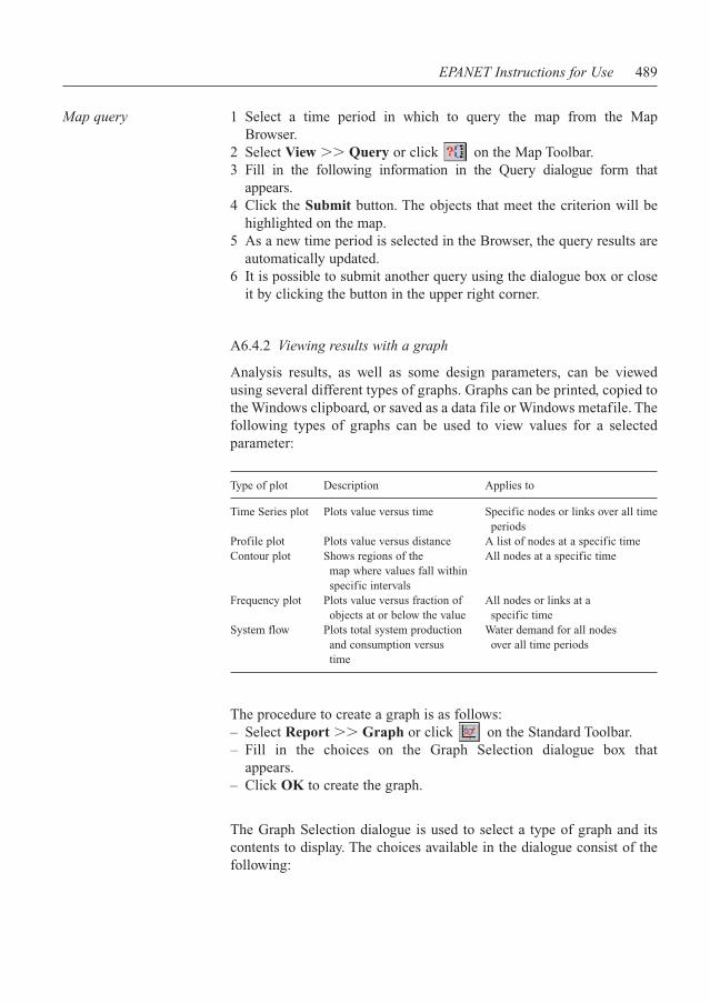
The procedure to create a graph is as follows:– Select Report Graph or click on the Standard Toolbar.– Fill in the choices on the Graph Selection dialogue box that
appears.– Click OK to create the graph.
The Graph Selection dialogue is used to select a type of graph and itscontents to display. The choices available in the dialogue consist of thefollowing:
490 Introduction to Urban Water Distribution
Item Description
Graph type Selects a graph typeParameter Selects a parameter to graphTime period Selects a time period to graph (does not apply to Time Series plots)Object type Selects either Nodes or Links (only Nodes can be graphed on Profile
and Contour plots)Items to graph Selects items to graph (applies only to Time Series and Profile plots)
Time Series plots and Profile plots require one or more objects beselected for plotting. The procedure to select items into the GraphSelection dialogue for plotting is as follows:– Select the object (node or link) either on the Network Map or on the
Data Browser. (The Graph Selection dialogue will remain visibleduring this process).
– Click the Add button on the Graph Selection dialogue to add theselected item to the list.
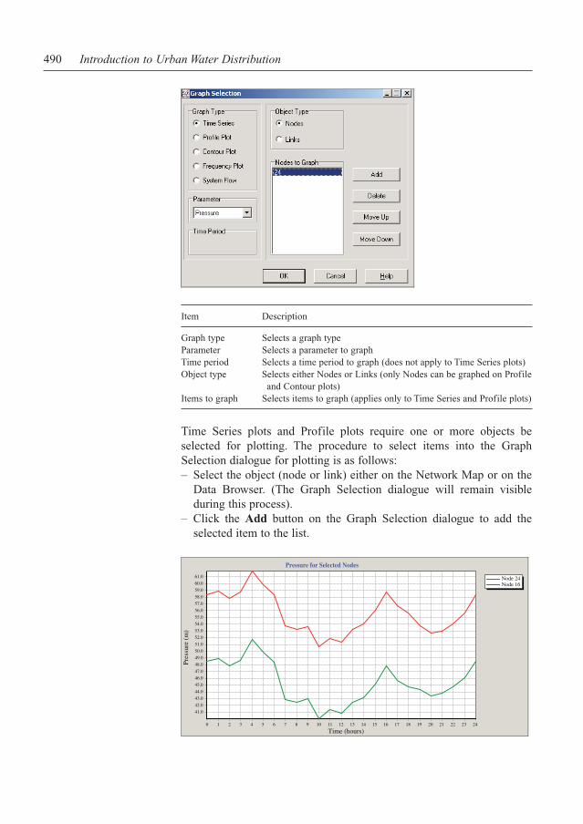
Node 24Node 16
Pressure for Selected Nodes
Time (hours)
Pres
sure
(m
)
61.0
59.0
60.0
58.0
57.0
56.0
55.0
54.0
53.0
52.0
51.0
50.0
49.0
48.0
47.0
46.0
45.0
44.0
43.0
42.0
41.0
0 1 2 3 4 5 6 7 8 9 10 11 12 13 14 15 16 17 18 19 20 21 22 23 24
EPANET Instructions for Use 491
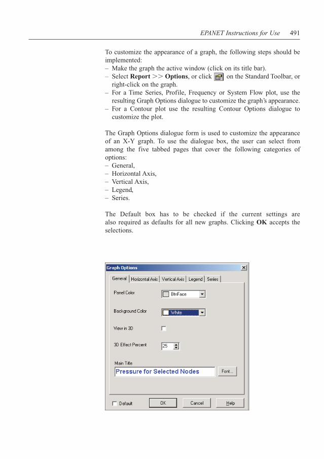
To customize the appearance of a graph, the following steps should beimplemented:– Make the graph the active window (click on its title bar).– Select Report Options, or click on the Standard Toolbar, or
right-click on the graph.– For a Time Series, Profile, Frequency or System Flow plot, use the
resulting Graph Options dialogue to customize the graph’s appearance.– For a Contour plot use the resulting Contour Options dialogue to
customize the plot.
The Graph Options dialogue form is used to customize the appearanceof an X-Y graph. To use the dialogue box, the user can select fromamong the five tabbed pages that cover the following categories ofoptions:– General,– Horizontal Axis,– Vertical Axis,– Legend,– Series.
The Default box has to be checked if the current settings arealso required as defaults for all new graphs. Clicking OK accepts theselections.
492 Introduction to Urban Water Distribution
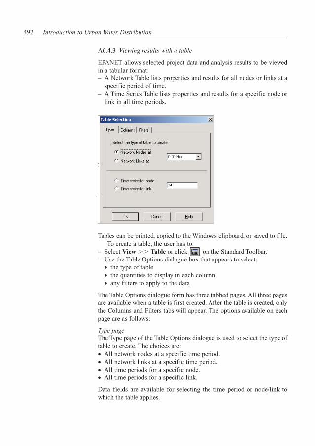
A6.4.3 Viewing results with a table
EPANET allows selected project data and analysis results to be viewedin a tabular format:– A Network Table lists properties and results for all nodes or links at a
specific period of time.– A Time Series Table lists properties and results for a specific node or
link in all time periods.
Tables can be printed, copied to the Windows clipboard, or saved to file.To create a table, the user has to:
– Select View Table or click on the Standard Toolbar.– Use the Table Options dialogue box that appears to select:
● the type of table● the quantities to display in each column● any filters to apply to the data
The Table Options dialogue form has three tabbed pages. All three pagesare available when a table is first created. After the table is created, onlythe Columns and Filters tabs will appear. The options available on eachpage are as follows:
Type pageThe Type page of the Table Options dialogue is used to select the type oftable to create. The choices are:● All network nodes at a specific time period.● All network links at a specific time period.● All time periods for a specific node.● All time periods for a specific link.
Data fields are available for selecting the time period or node/link towhich the table applies.
EPANET Instructions for Use 493
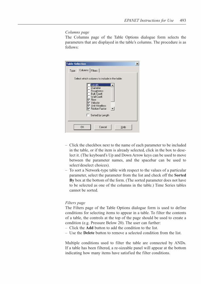
Columns pageThe Columns page of the Table Options dialogue form selects theparameters that are displayed in the table’s columns. The procedure is asfollows:
– Click the checkbox next to the name of each parameter to be includedin the table, or if the item is already selected, click in the box to dese-lect it. (The keyboard’s Up and Down Arrow keys can be used to movebetween the parameter names, and the spacebar can be used toselect/deselect choices).
– To sort a Network-type table with respect to the values of a particularparameter, select the parameter from the list and check off the SortedBy box at the bottom of the form. (The sorted parameter does not haveto be selected as one of the columns in the table.) Time Series tablescannot be sorted.
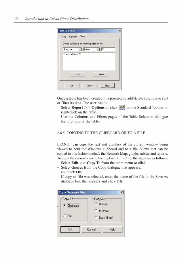
Filters pageThe Filters page of the Table Options dialogue form is used to defineconditions for selecting items to appear in a table. To filter the contentsof a table, the controls at the top of the page should be used to create acondition (e.g. Pressure Below 20). The user can further:– Click the Add button to add the condition to the list.– Use the Delete button to remove a selected condition from the list.
Multiple conditions used to filter the table are connected by ANDs.If a table has been filtered, a re-sizeable panel will appear at the bottomindicating how many items have satisfied the filter conditions.
494 Introduction to Urban Water Distribution
Once a table has been created it is possible to add/delete columns or sortor filter its data. The user has to:– Select Report Options or click on the Standard Toolbar or
right-click on the table.– Use the Columns and Filters pages of the Table Selection dialogue
form to modify the table.
A6.5 COPYING TO THE CLIPBOARD OR TO A FILE
EPANET can copy the text and graphics of the current window beingviewed to both the Windows clipboard and to a file. Views that can becopied in this fashion include the Network Map, graphs, tables, and reports.To copy the current view to the clipboard or to file, the steps are as follows:– Select Edit Copy To from the main menu or click.– Select choices from the Copy dialogue that appears.– and click OK.– If copy-to-file was selected, enter the name of the file in the Save As
dialogue box that appears and click OK.

Use the Copy dialogue as follows to define how data is to be copied andto where:– Select a destination for the material being copied (Clipboard or File).– Select a format to copy in:
● Bitmap (graphics only)● Metafile (graphics only)● Data (text, selected cells in a table, or data used to construct a
graph)● Click OK to accept the selections or Cancel to cancel the copy
request.
A6.6 ERROR AND WARNING MESSAGES
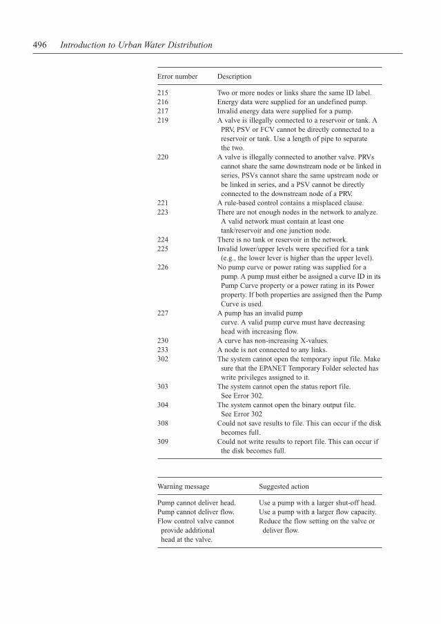
Error number Description
101 An analysis was terminated due to insufficient memoryavailable.
110 An analysis was terminated because the networkhydraulic equations could not be solved. Check forportions of the network not having any physical linksback to a tank or reservoir or for unreasonable valuesfor network input data.
200 One or more errors were detected in the input data. Thenature of the error will be described by the 200-serieserror messages listed below.
201 There is a syntax error in a line of the input file createdfrom the network data. This is most likely to haveoccurred in .INP text created by a user outside ofEPANET.
202 An illegal numeric value was assigned to a property.203 An object refers to undefined node.204 An object refers to an undefined link.205 An object refers to an undefined time pattern.206 An object refers to an undefined curve.207 An attempt is made to control a check valve. Once a
pipe is assigned a Check Valve status with the Property Editor, its status cannot be changed by either simple or rule-based controls.
208 Reference was made to an undefined node. This couldoccur in a control statement for example.
209 An illegal value was assigned to a node property.210 Reference was made to an undefined link. This could
occur in a control statement for example.211 An illegal value was assigned to a link property.212 A source tracing analysis refers to an undefined trace
node.213 An analysis option has an illegal value (an example
would be a negative time step value).214 There are too many characters in a line read from an
input file. The lines in the .INP file are limited to 255characters.
EPANET Instructions for Use 495
496 Introduction to Urban Water Distribution
Error number Description
215 Two or more nodes or links share the same ID label.216 Energy data were supplied for an undefined pump.217 Invalid energy data were supplied for a pump.219 A valve is illegally connected to a reservoir or tank. A
PRV, PSV or FCV cannot be directly connected to areservoir or tank. Use a length of pipe to separate the two.
220 A valve is illegally connected to another valve. PRVscannot share the same downstream node or be linked inseries, PSVs cannot share the same upstream node orbe linked in series, and a PSV cannot be directlyconnected to the downstream node of a PRV.
221 A rule-based control contains a misplaced clause.223 There are not enough nodes in the network to analyze.
A valid network must contain at least onetank/reservoir and one junction node.
224 There is no tank or reservoir in the network.225 Invalid lower/upper levels were specified for a tank
(e.g., the lower lever is higher than the upper level).226 No pump curve or power rating was supplied for a
pump. A pump must either be assigned a curve ID in itsPump Curve property or a power rating in its Powerproperty. If both properties are assigned then the PumpCurve is used.
227 A pump has an invalid pumpcurve. A valid pump curve must have decreasing head with increasing flow.
230 A curve has non-increasing X-values.233 A node is not connected to any links.302 The system cannot open the temporary input file. Make
sure that the EPANET Temporary Folder selected haswrite privileges assigned to it.
303 The system cannot open the status report file. See Error 302.
304 The system cannot open the binary output file. See Error 302
308 Could not save results to file. This can occur if the diskbecomes full.
309 Could not write results to report file. This can occur ifthe disk becomes full.
Warning message Suggested action
Pump cannot deliver head. Use a pump with a larger shut-off head.Pump cannot deliver flow. Use a pump with a larger flow capacity.Flow control valve cannot Reduce the flow setting on the valve orprovide additional deliver flow.head at the valve.
EPANET Instructions for Use 497
A6.7 TROUBLESHOOTING RESULTS
Pumps cannot deliver flow or head
EPANET will issue a warning message when a pump is asked to operateoutside the range of its pump curve. If the pump is required to delivermore head than its shut-off head, EPANET will close down the pump.This might lead to portions of the network becoming disconnectedi.e. without any source of supply.
Network is disconnected
EPANET classifies a network as being disconnected if there is no way toprovide water to all nodes that have demands. This can occur if there isno path of open links between a junction with demand and either a reser-voir, a tank, or a junction with a negative demand. If the problem iscaused by a closed link EPANET will still compute a hydraulic solution(probably with extremely large negative pressures) and attempt to iden-tify the problem link in its Status Report. If no connecting link(s) exist,EPANET will be unable to solve the hydraulic equations for flows andpressures and will return an Error 110 message where an analysis will bemade. Under an extended period simulation it is possible for nodes tobecome disconnected as links change status over time.
Negative pressures exist
EPANET will issue a warning message when it encounters negativepressures at junctions that have positive demands. This usually indicatesthat there is some problem with the way the network has been designedor operated. Negative pressures can occur when portions of the networkcan only receive water through links that have been closed off. In suchcases an additional warning message about the network being discon-nected is also issued.
System unbalanced
A System unbalanced condition can occur when EPANET cannotconverge to a hydraulic solution in some time period within its allowedmaximum number of trials. This situation can occur when valves,pumps, or pipelines keep switching their status from one trial to thenext as the search for a hydraulic solution proceeds. For example, thepressure limits that control the status of a pump may be set too closetogether, or the pump’s head curve might be too flat causing it to keepshutting on and off.
To eliminate the unbalanced condition it is possible to try to increasethe allowed maximum number of trials or loosen the convergenceaccuracy requirement. Both of these parameters are set with the project’sHydraulic Options. If the unbalanced condition persists, then anotherhydraulic option, labelled ‘If Unbalanced’, offers two ways to handle it.One is to terminate the entire analysis once the condition is encountered.The other is to continue seeking a hydraulic solution for another 10 tri-als with the status of all links frozen to their current values. If conver-gence is achieved then a warning message is issued about the systempossibly being unstable. If convergence is not achieved then a ‘SystemUnbalanced’ warning message will be issued. In either case, the analysiswill proceed to the next time period.
If an analysis in a given time period ends with the system unbalanced,then the user should recognize that the hydraulic results produced for thistime period are inaccurate. Depending on circumstances, such as errorsin flows into or out of storage tanks, this might affect the accuracy ofresults in all future periods as well.
Hydraulic equations unsolvable
Error 110 is issued if at some point in an analysis the set of equationsthat model flow and energy balance in the network cannot be solved.This can occur when some portion of a system demands water but has nolinks physically connecting it to any source of water. In such a caseEPANET will also issue warning messages about nodes being discon-nected. The equations might also be unsolvable if unrealistic numberswere used for certain network properties.
498 Introduction to Urban Water Distribution