Equity market fragmentation and liquidity: the

impact of MiFID

(Preliminary)

Hans Degryse� Frank de Jongy Vincent van Kervelz

January 2011

Abstract

Changes in European �nancial regulation (the Markets in Financial Instru-

ments Directive) in November 2007 allow new trading venues to emerge and

compete with traditional stock exchanges (regulated markets). As a result,

currently, many stocks are traded on a multitude of trading platforms, i.e. the

market has become fragmented. This paper evaluates the impact of fragmenta-

tion on liquidity for a sample of 52 Dutch stocks. We consider global liquidity

by aggregating order book information over all European trading venues and

incorporating the depth of the entire order books, and local liquidity by consid-

ering the regulated market only. Controlling for stock characteristics and time

e¤ects, we �nd that global liquidity increases with fragmentation, but these

bene�ts are not enjoyed by all investors as local liquidity reduces.

JEL Codes: G10; G14; G15;

Keywords: Market microstructure, Market fragmentation, Liquidity, MiFID

zCentER, EBC, TILEC, Tilburg University. TILEC-AFM Chair on �nancial market regulation.zCentER, Tilburg UniversityzCorresponding author, TILEC, CentER, Tilburg University, Email: v.l.vankervel@uvt.nl.

The authors thank Mark Van Achter and Gunther Wuyts, and participants at the 2010 Erasmusliquidity conference (Rotterdam), the K.U. Leuven, the 2010 AFM workshop on MiFID (Amsterdam)and Tilburg University for helpful comments and suggestions.

1

I Introduction

Following the developments in the U.S., European equity markets have seen a prolifer-

ation of new trading venues. While traditional stock exchanges had a near monopoly

on trading until the beginning of 2007, recent changes in �nancial regulation, in

particular the Markets in Financial Instruments Directive (MiFID), allow new trad-

ing venues to compete for order �ow. Consequently, trading has become dispersed

over many trading venues, creating a fragmented market place. How fragmentation of

trading a¤ects market quality, and liquidity in particular, has since long interested re-

searchers, regulators, investors and trading institutions. This question needs further

reconsideration as technological progress nowadays creates possibilities to connect

with di¤erent trading venues. In this paper, we shed new light on the matter and

improve upon previous research by employing a dataset that covers the relevant uni-

verse of trading platforms, provides stronger identi�cation and allows for improved

liquidity metrics.

In Europe, the fragmentation of trading is largely a consequence of the imple-

mentation of MiFID in November 2007. MiFID�s main goal is to improve market

quality through two channels; by introducing competition between trading venues

and by imposing similar degrees of transparency across most trading venues. First,

di¤erent types of trading venues are allowed to compete for order �ow with the tra-

ditional market. This is expected to reduce the monopoly power of the traditional

market, to lower transaction costs (Biais, Martimort, and Rochet, 2000) and to foster

technological innovation (Stoll, 2003). However, there is also evidence that fragmen-

tation might reduce liquidity. When order �ow becomes fragmented, the probability

of �nding a counterparty diminishes. Consequently, execution probabilities are low-

ered, which might cause some investors to leave the market or informed investors to

leverage their informational advantage (e.g. Chowdhry and Nanda (1991)). More-

over, a single, consolidated market may enjoy economies of scale resulting in lower

processing costs. Second, in order to create a fair level playing �eld, most trading

venues have to comply with similar enhanced transparency requirements. In particu-

lar, trading venues are requested to report continuously on executed transactions and

on the quotes they o¤er.1 When transparency enhances, information can be accessed

1An exception of the pre-trade transparency regulation is granted to so-called dark pools, assuch rules would con�ict with their business model.

2

faster and cheaper, hence improving e¢ ciency (e.g. Boehmer, Saar, and Yu (2005)).

This paper adds to the literature by investigating the impact of fragmentation on

liquidity. Foucault and Menkveld (2008) study competition between the LSE and Eu-

ronext, using data from 2004, and �nd that fragmentation over these two traditional

stock markets improves liquidity. O�Hara and Ye (2009) �nd that fragmentation low-

ers transaction costs and increases execution speeds for NYSE and NASDAQ stocks.

In this paper, we investigate the impact of competition by new trading venues on

market liquidity for a sample of European stocks in the period after the introduction

of MiFID.

In contrast to the U.S., the impact in Europe may be a¤ected by di¤erent regula-

tory requirements on executed trades. Speci�cally, European brokers are required to

execute trades against the best available conditions with respect to price, liquidity,

transaction costs and likelihood and speed of execution.2 A consequence of this broad

de�nition of execution quality is that European brokers can de�ne the best-execution

benchmark themselves, and may even choose to trade on one trading venue only,

typically the traditional exchange. As such, price violations can occur, i.e. a trade

is executed at a price worse than the best price available in the market. In the U.S.

however, trading venues are obliged to execute trades against the best price available

in the market (the National Best Bid or O¤er, NBBO). Stoll (2006) argues that this

rule is controversial as forcing �rms to compete primarily on prices undermines the

other dimensions of execution quality. An advantage of the trade-through rule is that

new entrants are guaranteed to attract order �ow when they have the best price in

the market, which is not necessarily the case in Europe. This seemingly small de-

viation in regulation can have substantial e¤ects on the competitive nature of new

entrants (Gomber and Gsell, 2006). The current work con�rms that fragmentation

has substantially di¤erent consequences for global traders (with access to all trading

venues) and local traders (with access to the regulated market only).

We address the impact of fragmentation on market liquidity by creating per �rm

daily proxies of fragmentation and liquidity, employing information from all relevant

trading venues. Speci�cally, we study 52 Dutch stocks in a period before the start

that fragmentation has set in, until the end of 2009. For each stock, we construct

a consolidated limit order book (i.e., the limit order books of all trading venues

2Directive 2004/39 on markets in �nancial instruments [2004] O.J. L145/1.

3

combined) to get a complete picture of the global liquidity available in the market.

Based on the consolidated order book, we analyze liquidity at the best price levels,

but also deeper in the order book. This is important, as the e¤ect of fragmentation

on liquidity may not be identical at di¤erent price levels in the limit order book. Next

to global liquidity, we also address the impact of fragmentation on liquidity at the

traditional market, which represents local liquidity. Global liquidity is relevant for

global traders, i.e. traders that have access to all markets, whereas local liquidity is

relevant for local traders, i.e. traders that tap the traditional market only.

The panel dataset aims to identify an exogenous relation between liquidity and

fragmentation by means of �rm*quarter �xed e¤ects and instrumental variables re-

gressions. That is, the �rm*quarter dummies only allow for variation in fragmentation

and liquidity within a �rm-quarter. Hence, they provide robustness to self selection

issues, for example that competition might be higher for high volume and more liquid

stocks. In addition, the �rm*quarter dummies, at least partially, control for dynamic

interactions between market structure, competition in the market, the degree of frag-

mentation and liquidity. Finally, the results based on the �rm*quarter dummies are

more robust to time e¤ects such as the �nancial crisis. In the instrumental variables

regressions we use the daily average order size of the venues that trade the stock as

instruments for the degree of fragmentation. This approach solves self selection issues

if we assume that the variation in fragmentation generated by the instruments is not

related to �rm size and initial level of liquidity, given the control variables already in

the regression.

Our main �nding is that there exists an inverted U-shape in the e¤ect of frag-

mentation on global liquidity, where the optimal level of fragmentation employing our

most conservative estimates improves depth with approximately 32% compared with

a completely concentrated market. Interestingly, this improvement holds for liquidity

close to the midpoint, i.e. at relatively good price levels, but to a much lesser extent

for liquidity deeper in the order book, which improves by only 12%. This result sug-

gests that new entrants mainly improve liquidity close to the midpoint, but do not

provide much liquidity deeper in the order book. While global liquidity bene�ts from

fragmentation, the traditional stock exchange is worse o¤ as local liquidity at good

price levels reduces by approximately 10%. This is in contrast to the result of Weston

(2002), who �nds that the introduction of ECNs improves liquidity on the primary

exchange. Finally, competition between trading venues is �ercer for large stocks then

4

for small stocks, as large stocks are more fragmented and bene�t twice as much from

fragmentation. In addition, the negative e¤ect of fragmentation on local liquidity is

only experienced by the small stocks.

These results suggest that local traders who only trade at the traditional stock

market, i.e. do not use Smart Order Routing Technology, can be worse o¤ in a

fragmented market, especially for relatively small orders. This conclusion adds to the

policy debate on the bene�ts and drawbacks of stock market fragmentation, where

fragmentation appears to have a bene�cial e¤ect on total market quality, but is not

equally enjoyed by all stock market participants.

The remainder of this paper is structured as follows. Section II describes the Eu-

ropean �nancial market after the introduction of MiFID. Section III discusses related

literature and challenges in estimating fragmentation and liquidity. The dataset and

liquidity measures are described in sections IV and V, while section VI explains the

methodology and results. Finally, the conclusion is presented in section VII.

II Background on European �nancial markets af-

ter MiFID

This section gives a brief discussion on the contents of the Markets in Financial

Instruments Directive (MiFID), e¤ective November 1, 2007. By implementing a single

legislation for the European Economic Area, MiFID aims to create a level playing �eld

for trading venues and investors, which would ultimately improve market quality. The

regulation entails three major changes to achieve this goal.

First, competition between trading venues is introduced by abolishing the �con-

centration rule�3 and allowing three types of trading systems to compete for order

�ow. These are regulated markets (RMs), Multilateral Trading Facilities (MTFs) and

Systematic Internalisers (SIs). RMs are the traditional exchanges, matching buyers

and sellers through an order book or through dealers. A �rm chooses on which RM

3The �concentration rule�, adopted by some EU members, obliges transactions to be executedat the primary market as opposed to internal settlement. This creates a single and fair market onwhich all investors post their trades, according to a time and price priority. The repeal of the rulehowever allows markets to become fragmented and increases competition between di¤erent tradingvenues (Ferrarini and Recine, 2006).

5

to list, and once listed, MTFs may decide to organize trading in that �rm as well.

MTFs are similar in matching third party investors, but have di¤erent regulatory

requirements and �rules of the game�. For example, MTFs and RMs can decide upon

the type of orders that can be placed, and the structure of fees, i.e. �xed fees,

variable fees as well as make or take fees.4 Typically, MTFs receive order �ow from

their owners or founders, generating some liquidity. But in order to survive, they

should attract order �ow from outside investors as well. In terms of traded volume,

the most important MTFs with visible liquidity are Chi-X, Bats Europe, NASDAQ

OMX and Turquoise. While SIX Swiss exchange is a regulated market, it took over

the MTF Virt-X in March 2008, which traded Eurostoxx 50 constituents.

Lastly, SIs are organized by investment banks where customers trade against the

inventory of the SI or with other clients (Davies, Dufour, and Scott-Quinn, 2006).

MiFID allows for new trading platforms and MiFID has at least partially succeeded

here. For example, market shares of the primary exchanges in Eurostoxx 50 stocks

have reduced from 100% in January 2008 to 78% in December 2009 (Gomber and

Pierron, 2010).

MiFIDs second keystone refers to transparency and guarantees the �ow of infor-

mation in the market. As the number of trading venues increases, information about

available prices and quantities in the order books becomes dispersed. However, in

order for investors to decide on the optimal venue and to evaluate order execution, a

su¢ cient degree of pre-trade and post-trade transparency is required. In particular,

to allow for comparisons between trading venues, pre-trade transparency rules are

set in, where trading venues are required to make (part of) their order books public

and to continuously update this information. A number of waivers exist regarding

pre-trade transparency. In particular, there is the �large-in-scale orders waiver�, the

�reference price waiver�, the �negiotated-trade waiver�, and the �order management

facility waiver�. These waivers are used for example by MTFs with completely hidden

liquidity, known as dark pools, who only have to report executed trades. Also, SIs do

not have to report their quotes for illiquid stocks.5

4Make and take fees are costs charged to investors supplying and removing liquidity, respectively.Make fees can be negative, such that providers of liquidity receive a rebate for o¤ering liquidity.

5A liquid stock is de�ned by the European Commission as having a free �oat market capitaliza-tion exceeding e500 million and an average daily trading activity of more than 500 trades Ferrariniand Recine (2006). The stock has to be listed on a regulated markets as well.

6

The third and �nal pillar of MiFID is the introduction of the best-execution rule,

which obliges investment �rms to execute orders against the best available conditions

with respect to price, liquidity, transaction costs and likelihood and speed of execution

(Aubry and McKee, 2007). However, such a broad de�nition of best-execution policy

allows investment �rms to decide themselves where to route their orders to. For

example, an investment �rm may stipulate an execution policy that compares prices

with one market only. In absence of a clear benchmark, it becomes di¢ cult for an

investor to evaluate the quality of executed trades and the overall performance of an

investment �rm (Gomber and Gsell, 2006). This is the main di¤erence between MiFID

and its U.S. counterparty, Reg NMS, which only focusses on execution prices.6 For an

extensive summary of the implementation process of MiFID we refer the interested

reader to Ferrarini and Recine (2006).

III Fragmentation and market quality

A Related literature

The following subsections summarize the literature on order �ow fragmentation and

competition. There is a trade-o¤ between a single consolidated market and a frag-

mented market. A single market bene�ts from lower costs, compared with a frag-

mented market. These consist of the �xed costs to set up a new trading venue; �xed

costs for clearing and settlement; costs of monitoring several trading venues simulta-

neously; and advanced technological infrastructure to aggregate dispersed information

in the market and connect to several trading venues. Also, a single market that is

already liquid will attract even more liquidity due to positive network externalities

(e.g. Pagano (1989a), Pagano (1989b) and Admati, Amihud, and P�eiderer (1991)).

Each additional trader reduces the stock�s execution risk for other potential traders,

attracting more traders. This positive feedback should cause all trades to be executed

at a single market, obtaining the highest degree of liquidity.

However, while network externalities are still relevant, nowadays they may be

realized even when several trading venues coexist. This happens to the extent that the

6In the U.S., the price of every trade is reported to the consolidated tape, such that the perfor-mance of a broker can clearly be evaluated.

7

technological infrastructure seamlessly links the individual trading venues, creating

e¤ectively one market. From a broker�s point of view, the market is then virtually

not fragmented, which alleviates the drawbacks of fragmentation (Stoll, 2006). In

addition, fragmentation might also enhance market quality, as increased competition

among liquidity suppliers forces them to improve their prices, narrowing the bid-ask

spreads (e.g. Biais, Martimort, and Rochet (2000) and Battalio (1997)). Con�rming a

competition e¤ect, Conrad, Johnson, and Wahal (2003) �nd that Alternative Trading

Systems in general have lower execution costs compared with traditional brokers.

Furthermore, Biais, Bisiere, and Spatt (2010) investigate the competition induced by

ECN activity on NASDAQ stocks. They �nd that ECNs with smaller tick sizes, tend

to undercut the NASDAQ quotes and reduce overall quoted spreads.

Di¤erences between trading venues may arise to cater to the needs of heteroge-

neous clientele, as investors di¤er in their preferences for trading speed, order sizes,

anonymity and likelihood of execution (Petrella, 2009; Harris, 1993). In the U.S.,

Boehmer (2005) stresses the trade-o¤ between speed of execution and execution costs

on NASDAQ and NYSE, where NASDAQ is more expensive but also faster. In order

to attract more investors, new trading venues may apply aggressive pricing schedules,

such as make and take fees. Foucault, Kadan, and Kandel (2009) model that asym-

metric make and take fees (i.e. liquidity takers pay a higher take fee than liquidity

makers receive as make fee) enhance trading activity. The fact that some investors

prefer a particular trading venue can also lead to varying degrees of informed trading

at each exchange. For instance, the NYSE has been found to attract more informed

order �ow than the regional dealers (Easley, Kiefer, and O�Hara, 1996) and NAS-

DAQ market makers (Bessembinder and Kaufman (1997) and A­ eck-Graves, Hedge,

and Miller (1994)). Furthermore, Barclay, Hendershott, and McCormick (2003) �nd

that ECNs attract more informed order �ow than NASDAQ market makers, as ECN

trades have a larger price impact.

Stoll (2003) argues that competition fosters innovation and e¢ ciency, but priority

rules may not be maintained. Speci�cally, time priority is often violated in fragmented

markets, and sometimes also price priority.7 Foucault and Menkveld (2008) study the

competition between an order book run by the LSE (EuroSETS) and Euronext Ams-

7Time priority is violated when two limit orders with the same price are placed on two venuesand the order placed last is executed �rst. Price priority is violated, i.e. a trade-through, whenan order gets executed against a price worse than the best quoted price in the market. A partialtrade-through means that only part of the order could have been executed against a better price.

8

terdam for AEX �rms in 2004, and �nd a trade-through rate of 73%. They call for a

prohibition of trade-throughs as it discourages liquidity provision. More recently, this

has been studied by Ende, Gomber, and Lutat (2010) as well, who combine the order

books of ten trading venues for Eurostoxx 50 stocks in December 2007 and January

2008. They �nd that 6.7% of all transactions are full trade-throughs and an addi-

tional 6.5% are partial trade-throughs. The authors provide two explanations for this

result. First, brokers might economize on monitoring costs and discard information

on available prices in some trading venues, i.e. do not use Smart Order Routing Tech-

nology. Second, trading charges and other fees such as clearing and settlement can

either make it more expensive to trade at the market o¤ering higher visible liquidity,

or make it expensive to split up an order among several venues (Degryse, van Achter,

and Wuyts, 2010). These explicit transaction costs as well as make and take fees

are not taken into account in the combined order book, while they do contribute to

the investors execution costs. If the role of explicit transaction costs is large enough,

investor could not have done better and in a broad sense, there is no trade-through.

Finally, this paper is related to the literature on algorithmic trading,8 i.e. the use

of computer programs to manage and execute trades in electronic limit order books.

Algorithmic trading has strongly increased over time, and has drastically a¤ected the

trading environment (Hendershott and Riordan, 2009). In particular, it a¤ects the

level of market fragmentation analyzed in our sample, as computer programs and

Smart Order Routing Technology (SORT) allow investors to �nd the best liquidity in

the market by comparing the order books of individual venues.9 Moreover, algorithmic

trading is related to liquidity as it reduces implicit transaction costs by splitting

up a large order into many smaller ones (Hendershott, Jones, and Menkveld, 2010).

Programs are also used to identify deviations from the e¢ cient share price, by quickly

trading on information in the market or from other securities. Furthermore, programs

may provide liquidity when quoted spreads are large, e.g. when it is pro�table to do

so (Hendershott and Riordan, 2009). Hasbrouck and Saar (2009) describe ��eeting

orders�, a relatively new phenomenon in Europe and the U.S., where limit orders are

placed and cancelled within two seconds if they are not executed. The authors argue

that �eeting orders are part of an active search for liquidity and a consequence of

improved technology, more hidden liquidity and fragmented markets; three elements

8Algorithmic trading is also know as High Frequency Trading.9See e.g. Gomber and Gsell (2006) for a discussion on SORT and algorithmic trading in Europe.

9

that are strongly developing in the European trading landscape.

B Challenges in analyzing the impact of fragmentation

In estimating the impact of fragmentation on liquidity, several data and methodolog-

ical issues have to be solved. New solutions to these problems will place the current

paper within the closest related literature.

First, it is crucial to correctly measure the extent of fragmentation on a stock-by-

stock basis. We employ a Her�ndahl-Hirsmann Index (HHI; the sum of the squared

market shares) to measure how concentrated trading is over the di¤erent markets.

Our measure of fragmentation then equals 1-HHI which is zero in the absence of

fragmentation. We compute the HHI based on executed trades on all visible trading

venues. Furthermore, we control for the aggregate trading activity on all non-visible

order books such as dark pools, SIs and OTC.10 Our measure of fragmentation is

more accurate than that of O�Hara and Ye (2009), where the origin of trades are

classi�ed as either NASDAQ, NYSE or external. The main bene�ts of competition

in their paper arise from the external venues, but the degree of fragmentation among

those venues is unknown.

We create a panel dataset containing daily indicators of fragmentation and liquid-

ity on a stock-by-stock basis over a time period of four years. A panel dataset allows

us to control for �xed �rm, time and �rm*time e¤ects, and provides an accurate

identi�cation of the impact of fragmentation and liquidity. Such a setup improves

on O�Hara and Ye (2009), who do a cross sectional regression, ignoring the time se-

ries variation in liquidity and fragmentation. Moreover, this setup allows for more

�exibility than related papers such as Foucault and Menkveld (2008), Chlistalla and

Lutat (2009) and Hengelbroc (2010), who study the introduction of a new trading

venue (EuroSETS, Chi-X and Turquoise respectively). Speci�cally, these articles use

a binary variable, i.e. a dummy that equals one after the introduction of the new

venue, to estimate the e¤ect of fragmentation on liquidity. In our setting however,

this approach would su¤er from three problems. First, it assumes that the level of

fragmentation on other trading venues has no confounding e¤ects on the liquidity of

10This aggregate non-visible orderbook activity does not provide information on which platformthe trade took place. We therefore do not include it in our fragmentation indicator as it mayrepresent trades on one venue only or on a panoply of platforms.

10

the venues in consideration. Second, this approach ignores the cross sectional varia-

tion in fragmentation, where some �rms are more heavily traded on the new venue

than others. And third, the binary variable does not take into account that a new

trading venue might need time to grow and attract order �ow. Furthermore, the

market as a whole might need time to adjust to a new trading equilibrium, so time

series variation in fragmentation is also ignored. Fortunately, the setup of our panel

dataset allows for cross sectional and time series variation and analyzes all visible

trading venues.

A second challenge is to use an appropriate measure of liquidity. We employ

two di¤erent views on liquidity representing the view from a global trader or local

trader, respectively. First consider the view from a global trader. We capture global

liquidity by aggregating the limit order books of all individual trading venues to

obtain a consolidated order book. This is important, as a global trader can use

Smart Order Routing Technology (SORT) to access the liquidity of all trading venues

simultaneously, so the consolidated order book re�ects her real trading opportunities.

Based on the consolidated order book, we can construct the traditional liquidity

measures, such as the quoted, realized and e¤ective spreads. In addition, we improve

on the work of e.g. O�Hara and Ye (2009), Gresse (2010) and Hengelbroc (2010) by

estimating a liquidity measure based on the entire depth of the consolidated order

book. That is, our data set also includes limit orders further away from the best

quotes,11 which are used to construct a new depth measure. Analyzing depth beyond

the best quotes is important, as the e¤ect of fragmentation might be di¤erent for

liquidity close to the midpoint, compared with liquidity deeper in the order book.

Second, we also consider liquidity for a local trader. This represents the view of a

trader without access to SORT who trades on the traditional stock market. In that

case, we measure liquidity only based upon the order book of Euronext.

A third challenge is identi�cation: is the observed relation between fragmentation

and liquidity causal, or is fragmentation endogenous? Over the years, there may

exist dynamic interactions between market structure, competition in the market, the

degree of fragmentation and liquidity. For example, changes in market structure

will a¤ect competition and fragmentation over time, which in turn will a¤ect market

structure. However, long-term correlations between these forces will be absorbed by

11The data contains the ten highest bid and lowest ask prices and their associated quantities, foreach trading venue.

11

the aforementioned �rm*quarter dummies. In addition, the �rm*quarter dummies

provide additional robustness to time e¤ects such as the �nancial crisis, which a¤ected

some stocks more than others. Furthermore, we execute an instrumental variables

regression, as large and liquid stocks may endogenously self select to becoming more

fragmented. As instruments we use the average daily order size of the seven visible

trading venues that trade the stock. This approach assumes that, after controlling

for stock characteristics and �rm*quarter dummies, the average daily order size is

uncorrelated to any self selection e¤ects. For exactly this issue, O�Hara and Ye (2009)

execute a Heckman correction model to account for a potential bias. However, self

selection issues are arguably less severe in Europe than in the United States. That

is, a new trading venue in Europe typically starts with a test phase in which only

a few liquid �rms are traded; but will allow trading in all stocks of a certain index

simultaneously when it goes live, i.e. there is no selection bias. For example, Chi-

X had a two week test phase where the �ve largest AEX25 and DAX30 �rms were

traded, while Turquoise had a �ve week test phase where �ve large European stocks

where traded. This is in strong contrast to the U.S., where some �rms may self select

to be traded on many di¤erent platforms.

IV Market description, dataset and descriptive sta-

tistics

A Market description

Our dataset contains 52 Dutch stocks forming the constituents of the AEX Large and

Mid cap indices. Over time, all of them are traded on several trading platforms. In

broad terms, we can summarize the most important trading venues for these stocks

into three groups, which we describe shortly.

First, there are regulated markets (RMs), such as NYSE Euronext, LSE and

Deutsche Boerse. All these markets have an opening and closing auction, and in

between there is continuous and anonymous trading through the limit order book.

Since Euronext merged with NYSE in April 2007, the order books in Amsterdam,

Paris, Brussels and Lisbon act as a fully integrated and single market (Davies, 2008).

In our sample, the LSE and Deutsche Boerse are not very important as they attract

12

less than 1% of total order �ow.

Second, there are the new MTFs with visible liquidity, such as Chi-X, Bats Eu-

rope, NASDAQ OMX and Turquoise. Chi-X started trading AEX �rms in April

2007; Turquoise in August 2008 and Nasdaq OMX and Bats Europe in October 2008.

Whether these MTFs will survive depends on the current level of liquidity, but also

on the quality of the trading technology (e.g. the speed of execution), the number of

securities traded, make and take fees and clearing and settlement costs.

The third group contains MTFs with completely hidden liquidity (e.g. dark

pools), SIs and the Over The Counter market. Dark pools are waived from the

pre-trade transparency rules set out by the MiFID due to the nature of their busi-

ness model. Most dark pools employ a limit order book with similar rules as those

at Euronext for example. Other MTFs act as crossing networks, where trades are

executed against the midpoint on the primary market, and do not contribute to price

discovery. Gomber and Pierron (2010) report that the activity on dark pools and

OTC has been fairly constant for European equities in 2008 - 2009, where they ex-

ecute approximately 40% of total traded volume. We refer the interested reader to

Davies (2008) for a description of some of the individual trading venues.

B Dataset

Our dataset covers the AEX Large and Midcap constituents from 2006 to 2009, which

currently have 25 and 23 stocks respectively. An advantage of using both indices is

that we are able to follow stocks that switch. We remove stocks that are in the

sample for less than six months or do not have observations in 2008 and 2009, such

as Getronics, Pharming, Stork, Numico and ABN Amro. Due to some leavers and

joiners, our �nal sample has 52 stocks.

The data for the 52 AEX Large and Midcap constituents stem from the Thomson

Reuters Tick History Data base. This data source covers the seven most relevant

European trading venues in Dutch stocks, which have executed more than 99% of

the visible order �ow: Euronext, Chi-X, Deutsche Boerse, Turquoise, Bats trading,

NASDAQ OMX and SIX Swiss exchange (formerly known as Virt-X).12 We employ

12The order books of the LSE are discarded as those stocks are denoted in pennies instead ofEuros; which in essence are di¤erent assets. The remaining trading venues with visible liquidity

13

data from all these venues but collect them only during the trading hours of the

continuous auction of Euronext Amsterdam, i.e. between 09.00 to 17.30, Amsterdam

time. Therefore, data of the opening and closing auctions at these venues are not

included.13

Each stock-venue combination is reported in a separate �le and represents a single

order book. Every order book contains the ten best quotes at both sides of the market,

i.e. the ten highest bid and lowest ask prices and their associated quantities, summing

to 40 variables per observation.14 A new �state�of a stock-venue limit order book

is created when a limit order arrives, gets cancelled or when a trade takes place.

A trade is immediately reported and we observe its associated price and quantity,

as well as an update of the order book. Price and time priority rules apply within

each stock-venue order book, but not between venues. Furthermore, visible orders

have time priority over hidden orders. Hidden orders are not directly observed in the

dataset but are detected upon execution. Therefore, we have the same information

set as traders have, i.e. the visible part of the order book in a continuous fashion.

Our dataset also provides information on �dark trades�, i.e. trades at dark pools,

SIs and Over The Counter (including trades executed over telephone). These dark

trades are part of the Thomson Reuters dataset and reported by Markit Boat, a

MiFID-compliant trade reporting company. Although these dark data have several

issues (e.g. double reporting and missing or double corrections), we use it only as a

control variable in our empirical analysis.15 In addition, we also add the OTC and SI

trades reported separately in the MiFID post trade �les from Euronext, Xetra, LSE,

Chi-X and Stockholm. While we have information regarding price, quantity and time

of execution, we do not observe the identity of the underlying trading venue. We

nevertheless can include aggregate information on �dark trading�in our analysis.

attract extremely little order�ow for the �rms in our sample (e.g. NYSE, Milan stock exchange,PLUS group and some smaller MTFs).

13Unscheduled intra-day auctions are not identi�ed in our dataset. These auctions, triggered bytransactions that would cause extreme price movements, act as a safety measure and typically lastfor a few minutes. Given that we will work with daily averages of quote-by-quote liquidity measures,we assume that these auctions will not a¤ect our results.

14Part of the sample only has the best �ve price levels: Euronext before January 2008. Onlyliquidity deep in the order book is a¤ected. In section B.5 we execute the analysis on a yearly basis:the results are una¤ected.

15To solve these data issues, the Committee of European Securities Regulators (CESR) proposesto standardise the trade reporting rules in their technical report of October 2010 on post tradetransparency. http://www.cesr-eu.org/data/document/10_882.pdf

14

C Descriptive statistics

Figure 1 shows the evolution of the daily traded volume, aggregated over all AEX

Large and Mid cap constituents. The graph shows a steady increase in total trading

activity, which peaks around the beginning of 2008. Moreover, the dominance of

Euronext over its challengers is strong, but slowly decreasing over time. This pat-

tern is representative for all regulated markets trading European blue chip stocks, as

analyzed in Gomber and Pierron (2010). Finally, while Chi-X started trading AEX

�rms in April 2007, all MTFs together have attracted signi�cant order �ow only as of

August 2008 (4,5%). The slow start up shows that these venues need time to generate

trading activity.

In Table I, the characteristics of the di¤erent stocks and some descriptive statistics

are presented. There is considerable variation in �rm size (market capitalization),

price and trading volume. In the sample, 40 stocks have a market capitalization

exceeding one billion Euro, while the 12 remaining stocks have values above 100

million Euro. In order to estimate a stock�s volatility, we divide the trading day

into 34 �fteen-minute periods, and calculate the stock return of each period, based

on the spread midpoint at the beginning and end of that period. The standard

deviation of these stock returns are daily estimates of realized volatility.16 The table

also shows the average market share of Euronext and dark trades, which covers all

trades reported by Markit Boat and OTC from the regulated markets. The market

shares are percentages of executed trades as of November 2007 onwards, the period

for which Markit Boat data have become available in the dataset. According to our

data, 25% of all trades are dark; which can be split up into 29.4% for AEX large cap

�rms and 18.9% for mid cap �rms.

V Liquidity and fragmentation

A The consolidated order book

The goal of this paper is to analyze the impact of equity market fragmentation on

liquidity. We follow the approach of Gresse (2010) and distinguish between �global

16The use of realized volatility is well established, see e.g. Andersen, Bollerslev, Diebold, andEbens (2001).

15

traders� and �local traders�. For global traders, global liquidity applies as they

employ Smart Order Routing Technology (SORT) to access all trading venues simul-

taneously; so liquidity should be aggregated over these venues. However, for local

traders, representing small investors, SORT might be too expensive because of �xed

trading charges and costs of adopting this trading technology. We therefore also

compute local liquidity and assume that those local traders only have access to the

primary market. Empirically, SORT is not used by all investors (e.g. Ende, Gomber,

and Lutat (2010) and Foucault and Menkveld (2008)). To analyze the impact of

fragmentation for local and global investors, we relate fragmentation to liquidity of

the traditional and aggregated market, respectively. Here, Euronext Amsterdam is

the primary market and the consolidated order book the aggregated market.

To construct the consolidated order book, we follow the methodology of Chlistalla

and Lutat (2009) and Foucault and Menkveld (2008), based on snapshots of the limit

order book. A snapshot contains the ten best bid and ask prices and associated

quantities, for each stock-venue combination. Every minute we take snapshots of all

venues and �sum�the liquidity to obtain a stock�s consolidated order book. Therefore,

each stock has 510 daily observations (8.5 hours times 60 minutes), containing the

order books of the separate trading venues and the consolidated one.

B Depth(X) liquidity measure

Our rich dataset allows to construct a liquidity measure that incorporates the limit

orders beyond the best price levels; which we will refer to as the Depth(X). The

measure aggregates the Euro value of the number of shares o¤ered within a �xed

interval around the midpoint. Speci�cally, the midpoint is the average of the best bid

and ask price of the consolidated order book and the interval is an amount X = {10,

20, ..., 60} basis points relative to the midpoint.17 The measure is expressed in Euros

and calculated every minute. Equation 1 shows the calculation for the bid and ask side

separately, which are summed to obtain Depth(X). Depth(X) is constructed for the

consolidated order book and the traditional stock market (i.e., Euronext Amsterdam)

separately. De�ne price level j = f1; 2; :::; Jg on the pricing grid and the midpoint of17Foucault and Menkveld (2008) aggregate liquidity from one up to four ticks away from the

best quotes. This measure only looks at the depth dimension, but does not incorporate the pricedimension, like ours. Furthermore, we use basis points as tick sizes vary over time.

16

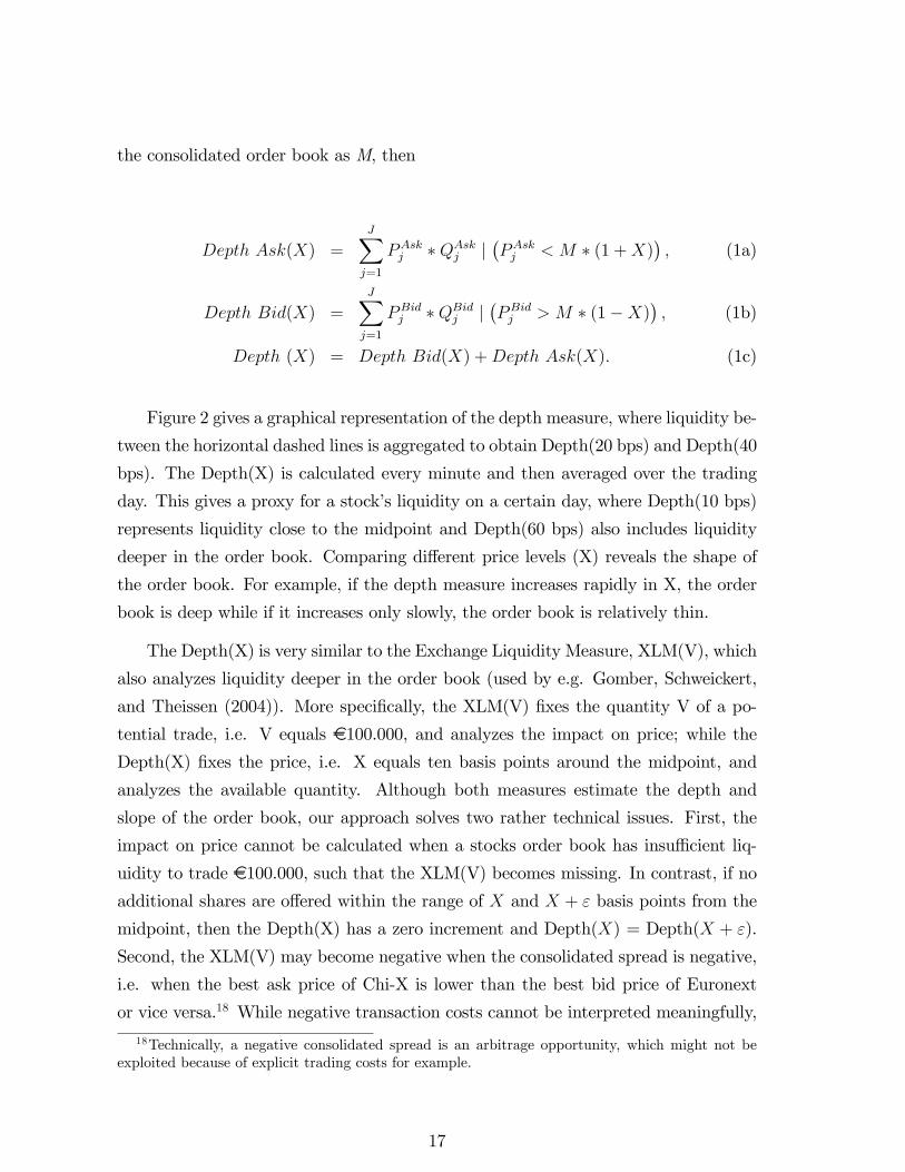
the consolidated order book as M, then

Depth Ask(X) =

JXj=1

PAskj �QAskj j�PAskj < M � (1 +X)

�; (1a)

Depth Bid(X) =JXj=1

PBidj �QBidj j�PBidj > M � (1�X)

�; (1b)

Depth (X) = Depth Bid(X) +Depth Ask(X): (1c)

Figure 2 gives a graphical representation of the depth measure, where liquidity be-

tween the horizontal dashed lines is aggregated to obtain Depth(20 bps) and Depth(40

bps). The Depth(X) is calculated every minute and then averaged over the trading

day. This gives a proxy for a stock�s liquidity on a certain day, where Depth(10 bps)

represents liquidity close to the midpoint and Depth(60 bps) also includes liquidity

deeper in the order book. Comparing di¤erent price levels (X) reveals the shape of

the order book. For example, if the depth measure increases rapidly in X, the order

book is deep while if it increases only slowly, the order book is relatively thin.

The Depth(X) is very similar to the Exchange Liquidity Measure, XLM(V), which

also analyzes liquidity deeper in the order book (used by e.g. Gomber, Schweickert,

and Theissen (2004)). More speci�cally, the XLM(V) �xes the quantity V of a po-

tential trade, i.e. V equals e100.000, and analyzes the impact on price; while the

Depth(X) �xes the price, i.e. X equals ten basis points around the midpoint, and

analyzes the available quantity. Although both measures estimate the depth and

slope of the order book, our approach solves two rather technical issues. First, the

impact on price cannot be calculated when a stocks order book has insu¢ cient liq-

uidity to trade e100.000, such that the XLM(V) becomes missing. In contrast, if no

additional shares are o¤ered within the range of X and X + " basis points from the

midpoint, then the Depth(X) has a zero increment and Depth(X) = Depth(X + ").

Second, the XLM(V) may become negative when the consolidated spread is negative,

i.e. when the best ask price of Chi-X is lower than the best bid price of Euronext

or vice versa.18 While negative transaction costs cannot be interpreted meaningfully,

18Technically, a negative consolidated spread is an arbitrage opportunity, which might not beexploited because of explicit trading costs for example.

17

the midpoint and Depth(X) are perfectly identi�ed and re�ect the available liquidity

in a meaningful fashion.

Figure 3 shows monthly averages of the Depth measure for 10 and 60 basis points

of Euronext Amsterdam and the consolidated order book, over the period 2006 to

2009. As expected, these measures covary strongly over time. However, some shocks

a¤ect liquidity close to the midpoint more than liquidity deep in the order book.

For example, when comparing the peak of liquidity in October 2007 to the low of

February 2008, the ratio of Depth(60 bps) to Depth(10 bps) doubles from 2.0 to 3.9.

This variation is present at the aggregate level and is also observed for most individual

�rms.

Finally, the upper panel of Figure 4 shows the shape of the order book by plotting

the median of the depth measure against the number of basis points around the

midpoint. The di¤erences between the medians reported here and the means of

Figure 3 are very large, a factor 3 to 5, which is in line with high levels of skewness and

kurtosis (not reported). Next to substantial variation over time (see Figure 3), there

also appear to be large di¤erences between �rms. For example, the 90th percentile of

Depth(10 bps) is e920.000, while the 10th percentile of Depth(60 bps) is e70.000. In

the regression analysis we will work with the logarithm of the depth measures, where

the 10, 50 and 90th percentiles are shown in the lower panel of Figure 4. Table II

contains the 25, 50 and 75th percentile of the Depth(X) measure on a yearly basis,

along with other liquidity measures discussed in the next section.

C Other liquidity measures

This section compares our Depth(X) liquidity measure to the more traditional liq-

uidity measures. These are the price impact, e¤ective and realized spread, based on

executed transactions, and the quoted spread and quoted depth, based on quotes

in the local and global order books. The quoted depth sums the Euro amount of

shares o¤ered at the best bid and ask price, whereas the quoted spread looks at the

associated prices. The appendix (section VIII) contains a formal description of these

measures.

The 25, 50 and 75th percentiles of the liquidity measures are reported in Ta-

ble II, based on daily observations and calculated yearly, for the consolidated order

18

book (upper panel) and Euronext Amsterdam (lower panel). The table shows several

interesting results.

Liquidity close to the midpoint has reduced strongly over time, while liquidity

deeper in the order book only marginally. That is, the median of Depth(10 bps) has

decreased by 35% from 2006 to 2009, while Depth(60 bps) by only 12%. In addition,

the yearly standard deviation of the depth measures has decreased by approximately

50% over the years (not reported).

Strikingly, between 2006 and 2009 the median quoted spread has improved by

10%, while the quoted depth has worsened by 68%. This result is in strong contrast

with the decrease of 35% in the Depth(10 bps) measure, and shows a shortcoming of

the quoted depth and spread. That is, based on the quoted depth and spread alone,

one cannot state whether an investor is better o¤ in 2006 or 2009, as this depends on

the size of his trade. For a small investor mainly the quoted spread matters, while

for a larger one the depth dimension becomes more important. To interpret these

numbers, one can argue that a trader who places an order smaller than the median

quoted depth in 2009, e30.000, is very likely to be better o¤ with on average 10%

(an argument similarly to that made in Hendershott, Jones, and Menkveld (2010)).

An additional advantage of the Depth(X) measure is that it is not sensitive to

small, price improving orders. For example, the strong reduction in quoted depth over

time might be explained by lowered tick sizes,19 or by increased activity of algorithmic

traders, who evidently place many small and price improving limit orders. The impact

of these phenomena on the quoted spread and depth also hinges on the degree of

fragmentation and may therefore vary over time, which makes comparisons between

periods troublesome. Finally, the Depth(X) measure can easily be aggregated over

several trading venues, while the quoted depth and spread are only aggregated if the

best bid and ask prices of the trading venues in consideration are identical.

Turning to the liquidity measures based on executed trades, we observe that the

median realized spread has reduced from 2.46 bps in 2006 to 0.02 bps in 2009. In this

period, the price impact went up with a 2.9 bps while the e¤ective spread reduced with

0.9 bps. Note that the price impact and realized spread together equal the e¤ective

spread. However, when calculating percentiles, each measure is ranked separately

19The e¤ect of the tick size on quoted depth and spread have been subject of analysis in severalpapers, e.g. Huang and Stoll (2001), Goldstein and Kavajecz (2000).

19

and as such they do not add up exactly. In addition, we have an unbalanced panel

because of �rms joining and leaving the sample.

The lower panel in Table II shows the same liquidity measures for the order book

of the traditional stock exchange, which represents the liquidity to a local investor.

While in 2006 and 2007 the numbers are highly similar to those of the consolidated

order book, in 2009 the Depth(X) on Euronext represents only about 50% of the

consolidated depth. In the same year, the quoted depth and spread on Euronext

Amsterdam are 20% and 9% worse compared to the consolidated order book.

Despite the reduction in Depth(X), the price impact, realized and e¤ective spread

are almost identical to that of the consolidated order book. This �nding might be

in line with �market tipping�, where Euronext switches between periods of relatively

high liquidity, in which it attracts all trading, and periods of low liquidity, in which

trading takes place at competing trading venues. As the price impact, e¤ective and

realized spread are based on trades, relatively liquid periods receive a larger weight

in the calculation.

D Equity market fragmentation

To proxy for the level of fragmentation in each stock, we construct a daily Her�ndahl-

Hirschman Index (HHI) based on the number of shares traded on each venue, similar

to Bennett and Wei (2006) and Weston (2002). HHIit =PN

v=1MS2v;it, or the squared

market share of venue v, summed over all N venues for �rm i on day t. A single

dominant market has an HHI close to one whereas HHI goes to zero in case of complete

fragmentation. In 2009, the average HHI of the sample �rms is 0.70, which is in line

with other European stocks analyzed by Gomber and Pierron (2010). The U.S. is more

fragmented, as NASDAQ and NYSE combined have approximately 65% of market

share in 2008, resulting in an HHI lower than 0.50 (O�Hara and Ye, 2009). Table

III shows the yearly mean, quartiles and standard deviation of HHI, based on the

sample �rms. As expected, the HHI declines over time, i.e. fragmentation increases.

Moreover, the standard deviation of HHI is fairly small in 2006 and 2007, as only few

sample �rms where traded on Virt-X, LSE and Deutsche Boerse.

The variation in HHI mainly stems from changes over time and to a lesser extent of

changes between �rms; i.e. the time series variation is larger than the cross sectional

20

variation. This result is shown in the lower part of Table III, where the standard

deviation of HHI is demeaned by �rm, by quarter and by �rm and quarter. That

is, from each observation we subtract o¤ the �rm average, or the quarterly average

or both, and report the standard deviation. As the table shows, demeaning by �rm

reduces the standard deviation with only 9% (0:135�0:1490:149

), while demeaning per quarter

reduces variation with 30%, so cross sectional variation is smaller than variation in

the time series.20 Finally, 43% of the total variation in fragmentation is captured by

adding both �rm and quarter dummies.

Figure 5 shows the 10, 50 and 90th percentile of HHI over time, calculated on

a monthly basis and covering all �rms. The sharp increase in fragmentation refers

to the period where Chi-X and Turquoise started to attract substantial order �ow,

September 2008. In the next section, we estimate the e¤ect of fragmentation on

various liquidity measures in a regression framework.

VI The impact of fragmentation on global and lo-

cal liquidity

A Methodology

We employ multivariate regression analysis to study the impact of fragmentation on

liquidity. We have a panel data set with N = 52 �rms and T = 1022 days (2006 �

2009), which contains the liquidity and fragmentation measures discussed in section

V. The Depth(X) is calculated for X = f10; 20; :::; 60g basis points. As the e¤ectof fragmentation on liquidity might not be linear, we add a quadratic term. To

ease the interpretation of the quadratic term, we will use Fragit = 1 � HHIit andFrag2it to measure fragmentation, where Fragit = 0 if trading in a �rm is completely

concentrated.

Control variables commonly used in this literature are the �rm characteristics de-

scribed in Table I.21 Furthermore, we control for algorithmic activity as this has been

20Indeed, as we have daily observations, demeaning per quarter still leaves some variation in thetime series. However, demeaning per day reduces the standard deviation with only 1% compared todemeaning per quarter.

21Weston (2000) and O�Hara and Ye (2009), among others, use similar controls.

21

found to improve liquidity (e.g. Hendershott and Riordan (2009)), where we construct

a measure similar to Hendershott, Jones, and Menkveld (2010). On average, algo-

rithmic traders place and cancel many limit orders, so the daily number of electronic

messages proxies for their activity, i.e. placement and cancellations of limit orders

and market orders. However, over time there is an increase in trading volume which

would lead to more electronic messages even in the absence of algorithmic traders.

To account for increasing trading volumes, the algorithmic trading proxy, Algoit; is

de�ned as the number of electronic messages divided by trading volume (in e100),

for �rm i on day t. Some descriptives of Algoit, and the additional control variables

Ln(V olatility)it; Darkit, Ln(Price)it; Ln(Size)it and Ln(V olume)it are presented in

Table IV. The regression equation becomes:

LiqMeasureit = Firmi + �1Fragit + �2Frag2it + �3Ln(V olatility)it +

�4Darkit + �5Ln(Price)it + �6Ln(Size)it + (2)

�7Ln(V olume)it + �8Algoit + "it:

In our base speci�cation, �rm �xed e¤ects and quarter dummies are included22

and in all regressions we use heteroskedasticity and autocorrelation robust standard

errors (Newey-West for panel datasets), based on �ve lags.

B Results

This subsection �rst presents our regression results for the base case (i.e., where we

include �rm �xed e¤ects and quarter dummies) for both the consolidated order book

and the traditional stock market. Later, we control for potential endogeneity issues

by introducing �rm*quarter e¤ects and two instrumental variables (IV) regressions.

The �rm*quarter dummies are aimed to control for the simultaneous interactions

between market structure, the degree of fragmentation, liquidity and competition in

the market. In the �rst instrumental variables regression we instrument the degree

of fragmentation of day t with that of t � 1, such that we remove the unexpecteddaily shocks from the variation in fragmentation. In the second IV regression we

instrument the degree of fragmentation by the average daily order size of each visible

venue that trades the stock. This approach may control for potential self selection

22The results are almost identical when using day or month dummies instead of quarter dummies.

22

issues, e.g. that competition tends to be higher for high volume and more liquid

stocks (Cantillon and Yin, 2010). We conclude by analyzing large and small �rms

separately, along with some additional robustness checks.

B.1 Regression analysis: base speci�cation

The regression results for the liquidity measures employing the consolidated order

book are reported in Table V. In Table VI, the same regressions are executed for

liquidity measures of the traditional stock market, Euronext Amsterdam. The latter

represents liquidity available to local investors, while the former liquidity to global

investors using SORT.

The coe¢ cients of Fragit and Frag2it (models (1) to (6), Table V) show that

liquidity �rst strongly increases with fragmentation and then starts to decrease as

the linear term has a positive coe¢ cient and the quadratic a negative one. The

results are easier to interpret when shown in a �gure where we display the implied

results for the six models representing di¤erent levels of depth. These are displayed

in Figure 6, with depth on the vertical axis and the level of fragmentation on the

horizontal axis.

The �gure clearly reveals a trade-o¤ in the bene�ts and downsides of fragmenta-

tion, where maximum liquidity is obtained at Frag = 0:35. This level of fragmenta-

tion is fairly close to the actual level observed in 2009 (where Frag is around 0:30).

The patterns are highly similar for all depth levels, although liquidity close to the

midpoint bene�ts more from fragmentation. The economic magnitudes of the vari-

ables are large, where the maximum e¤ect on Ln Depth(10 bps) is 0:50, meaning that

observations here have exp(0:50) = 1:65 or 65% more liquidity than observations in a

completely concentrated market. For Depth(60 bps), liquidity improves with 50% at

the maximum. The standard deviation of fragmentation is 0.15 in the entire sample

(Table III), so variation in fragmentation has a large impact on liquidity throughout

the entire order book.

We now investigate the impact of fragmentation on the other liquidity indicators

as reported in the remaining models from Table V. We observe the following in models

(7) to (9). The optimal degree of fragmentation (Frag = 0:35) reduces the price

impact and the e¤ective spread with 6:4 and 6:8 basis points in comparison with a

23

completely concentrated market. This is large, considering that the median e¤ective

spread in 2009 is 13:3 basis points. The economic impact of the optimal degree of

fragmentation on the e¤ective spread in our analysis is larger than the one estimated

in O�Hara and Ye (2009), where the bene�t is approximately three basis points for

NYSE and NASDAQ �rms.23 The e¤ect on the realized spread is much smaller with

a reduction of only 0.5 basis points.

In line with the other liquidity measures, the quoted spread is minimized at

Frag = 0:37 and is eight basis points lower compared with a completely concentrated

market (model (10)). This result is in stark contrast to the Ln quoted depth (model

(11)), which reduces with 27% at Frag = 0:37. The results on the quoted depth

point in the opposite direction of those of all other liquidity measures. Moreover,

considering the low correlation between the quoted depth and Depth(X) in Table II,

it appears that the quoted depth does not perform well in estimating liquidity over

longer periods of time.

Turning to the control variables of the regressions, we �nd that the economic

magnitude of Algoit is fairly small and negative. For example, a one standard devia-

tion increase (s = 0:36), lowers the Depth(X) measures with 4%. However, as Algoitmight be indirectly related to fragmentation, we want to be careful in interpreting

this result. The remaining control variables in the regressions have the expected signs.

Larger �rms tend to be more liquid, so the coe¢ cient on Ln size is positive and fairly

large. The e¤ect of price is marginally positive and economically very small. As ex-

pected, increased trading volumes are associated to better liquidity. Also, volatility

has a negative impact on liquidity; especially for liquidity close to the midpoint. Not

surprisingly, the price impact strongly increases in volatility, which proxies for the

amount of information in the market. The coe¢ cients on Darkit are strongly nega-

tive, where a one standard deviation increase (s = 0:18) reduces Depth(10 bps) with

17%. Possibly, dark trading venues gain liquidity at the expense of lit markets, as

they are substitutes. In addition, dark trades seem to be correlated to more informed

trading, as the coe¢ cient on the price impact is positive (4.13 bps).

The impact of fragmentation on liquidity for an investor not using SORT is shown

in Table VI. This table contains the regression results where our liquidity measures

23O�Hara and Ye (2009) �nd a linear coe¢ cient on �marketshare outside the primary markets�of9 basis points, while the average level is 0.35, resulting in a bene�t of approximately 3 basis points.

24

are based on the order book of Euronext Amsterdam only. To interpret the results,

we plot depth against fragmentation in Figure 7. Interestingly, Depth(10 bps) �rst

slightly improves with fragmentation, where the maximum lies at +10% at Frag =

0:17, but afterwards quickly reduces to -10% at Frag = 0:4. This reduction is in line

with the theory of Foucault and Menkveld (2008), where the execution probability

on Euronext diminishes as competing venues take away order �ow. This side e¤ect of

competition makes Euronext less attractive to liquidity providers, resulting in lower

depth.

Consequently, small investors, who mainly care for Depth(10 bps) and are limited

to trading on Euronext only, are worse o¤. This result is in contrast to Weston (2002)

for instance, who �nds that the liquidity on NASDAQ improves when ECNs enter

the market and compete for order �ow. Likely, the di¤erence is due to the market

structure in the U.S., where NASDAQ market makers lost their oligopolistic rents

after the entry of ECNs.

The di¤erence between the global and local order book represents the liquidity

available at the competing trading venues, who mainly o¤er liquidity at Depth(10 bps)

and to a much lesser extent at Depth(60). That is, at Frag = 0:40, the MTFs o¤er

44% of Depth(10 bps) and only 26% of Depth(60 bps).24 It appears that competition

mainly takes place at liquidity close to the midpoint.

We now turn to the regressions of the remaining liquidity measures in Table VI,

columns (7) - (11). Surprisingly, these are not adversely a¤ected by fragmentation.

That is, despite the reduction in Depth(10 bps), the price impact and e¤ective and

realized spread still improve with fragmentation. It might be the case that Euronext

is very liquid on some parts of the day, while relatively illiquid during other parts. As

the e¤ective spread is based on trades, more liquid periods with many trades receive

a larger weight in the calculation. In addition, order splitting behavior and smaller

average order sizes may also generate lower average e¤ective spreads.

Finally, the quoted spread on Euronext improves with fragmentation, while the

quoted depth reduces with 30% at Frag = 0:35. This means that the gains of

improved prices are more than o¤set by the lower quantities o¤ered, such that the

24At Frag = 0:40, the consolidated Depth(10 bps) is 63% higher than that of a completelyconcentrated market, while the local Depth(10 bps) is 8% lower. Therefore, the MTFs o¤er 163�92163 =44% of the global Depth(10 bps).

25

Depth(10 bps) has reduced.

B.2 Regression analysis: �rm*time e¤ects

In this section we do the regressions speci�ed in (2), but add �rm*quarter dummies.

Instead of a single dummy for a period of four years, we add 16 dummies per �rm.

This is similar to Chaboud, Chiquoine, Hjalmarsson, and Vega (2009), who analyze

the e¤ect of algorithmic trading on volatility for currencies, and add separate quarter

dummies for each currency pair. This procedure is aimed to solve the following issues.

First, the �rm*quarter dummies provide additional robustness to the impact of

the �nancial crisis and industry speci�c shocks. For example, if the �nancial crisis

speci�cally a¤ects certain �rms or industries (e.g. the �nancial sector), and a¤ects

both liquidity and fragmentation, then the previous analysis would su¤er from an

omitted variables problem, leading to a bias in the coe¢ cients on fragmentation.

However, the �rm*quarter dummies will capture industry shocks and time-varying

�rm speci�c shocks.

Second, the �rm*quarter dummies can control for potential self selection prob-

lems. For example, Cantillon and Yin (2010) raise the issue that competition might

be higher for high volume and more liquid stocks; an e¤ect that will be absorbed by

the �rm*quarter dummies.

Third, the �rm*quarter dummies can, at least partially, control for dynamic in-

teractions between market structure, competition in the market, the degree of frag-

mentation and liquidity. Speci�cally, such interactions are dynamic as, for example,

a change in the current market structure will a¤ect the level of competition in the

future, which, in turn, will a¤ect the market structure in the future. Our approach

controls for the long-term interactions of these forces by only allowing for variation in

liquidity and fragmentation within a �rm-quarter. Accordingly, the dummy variables

absorb the variation between quarters, which is likely to be more prone to endogeneity

issues.

The results for global liquidity reveal a similar pattern as those presented in the

original regressions, as shown in panel A of Table VII and displayed in Figure 8. For

the sake of brevity, the table does not report the coe¢ cients of the control variables

as these have the same signs and magnitudes as those reported in Tables V and VI,

26

but are available upon request.

In the �rst regression, we observe that Depth(10 bps) almost monotonically in-

creases with fragmentation. That is, the maximum of the parabola lies outside the

relevant domain, at Frag = 0:67, so there appears to be no harmful e¤ect of frag-

mentation on liquidity close to the midpoint. This is not the case for the other depth

levels, as the maximum lies around Frag = 0:40, implying a trade-o¤ in the bene�ts

and drawbacks of fragmentation.

In addition, two other �ndings emerge from the �gure. First, the magnitudes

of the coe¢ cients are about 45% to 75% lower, as Depth(10 bps) equals 0:28 at

Frag = 0:40; compared with 0:50 in Table V, while Depth(60 bps) is 0:10 com-

pared with the original 0:40 (but still highly signi�cant). This is likely because the

�rm*quarter dummies absorb long-term trends in the measure of fragmentation, while

the more noisy day-to-day �uctuations remain. From the regression results, it appears

that removing the long-term variation dampens the estimated daily e¤ects. Second,

liquidity deeper in the order book bene�ts less from fragmentation than liquidity close

to the midpoint does. This �nding was also con�rmed in Figure 6, but becomes more

pronounced. The fact that Depth(10 bps) still improves strongly in fragmentation is

in line with the earlier �nding that competition of new trading venues mainly takes

place at liquidity close to the midpoint.

Turning to the other liquidity measures in Table VII, columns (7) - (11), we

observe that the magnitudes of the coe¢ cients on fragmentation have diminished,

but in unreported plots all show a pattern similar to that of the base case.

The impact of fragmentation on local liquidity, including �rm*quarter e¤ects, is

shown in panel B of Table VII and Figure 9. The �gure shows that all the depth

measures reduce with fragmentation, while in the base speci�cation this only held

for Depth(10). However, not all coe¢ cients are signi�cant because the magnitude is

fairly close to zero while the 750 �rm*quarter dummies greatly reduce the statistical

power of the regressions. The fact that the coe¢ cients are close to zero can again

be attributed to the dummies, which absorb the long-term trends in fragmentation.

Similar to the previous subsection, we con�rm that the MTFs mainly o¤er liquidity at

Depth(10 bps), and to a much lesser extent at Depth(60). That is, following previous

calculations,24at Frag = 0:40, the MTFs o¤er 30% of Depth(10 bps) and only 15%

of Depth(60 bps). This is in line with MTFs who speci�cally compete on the price

27

dimension of liquidity.

B.3 An instrumental variables approach

The main focus of interest are the coe¢ cients of Fragi;t and Frag2i;t in equation (2),

but these are potentially biased, as discussed earlier. In order to further alleviate

potential endogeneity issues, we employ two instrumental variables speci�cations.

Formally, the set of instruments needs to be uncorrelated with the error term "it

(exogeneity of the instrument), and correlated to Fragi;t (a su¢ ciently strong instru-

ment).

In the �rst speci�cation, we instrument Fragi;t and Frag2i;t with their lagged

values Fragi;t�1 and Frag2i;t�1. The intuition is that potentially, an unexpected daily

shock can a¤ect liquidity and fragmentation simultaneously, resulting in a biased

coe¢ cient of fragmentation. Using Fragi;t�1 and Frag2i;t�1 as instruments removes

the unanticipated daily �uctuations in fragmentation.

In the second speci�cation, we instrument Fragi;t and Frag2i;t with the logarithm

of the average daily order size of the seven venues that trade the stock, resulting in

seven instruments. This speci�cation is aimed to control for a selection bias, where

for example large or highly traded �rms are more likely to become fragmented. For

this reason, O�Hara and Ye (2009) estimate a Heckman correction model. Here, the

seven instruments are only weakly related to liquidity, but can strongly predict frag-

mentation.25 As such, the instruments generate su¢ cient variation in fragmentation,

which, we argue, is unrelated to any self selection e¤ect. In both speci�cations, we

again add �rm*quarter dummies.

The results of the �rst speci�cation are shown in panel A (global liquidity) and

B (local liquidity) of Table VIII. Again, for the sake of brevity we do not report the

coe¢ cients of the control variables, as these have the same signs and magnitudes as

those reported in the base speci�cations.

First we notice that the coe¢ cients are highly similar to those reported in Table

V. At the optimal level of fragmentation, Frag = 0:35, global Depth(10 bps) im-

proves by 65% compared with a fully concentrated market. This is a consequence

25In all IV regressions the weak identi�cation test (or Paap-Kleibergen Wald test), is stronglyrejected.

28

of two o¤setting forces that are at play here. On the one hand, the addition of the

�rm*quarter dummies removes long-term trends in fragmentation, which are more

strongly related to liquidity and would lower the estimated coe¢ cients (as in the

previous section). On the other hand, by using Fragi;t�1 as instrument, we remove

the noisy day-to-day �uctuations in fragmentation, which are only weakly related to

liquidity. The two forces combined are o¤ setting, as plots of the results are almost

identical to those of the base speci�cation regressions (not reported). The coe¢ cients

in panel B are also very similar to the original ones, but not statistically di¤erent

from zero as the standard errors are strongly increased by the IV procedure. The

fact that the IV coe¢ cients are of the same sign and magnitude as the original ones,

shows that the part of fragmentation that is known in advance (i.e. the day before)

can explain the bene�cial e¤ect of fragmentation on liquidity. The coe¢ cients of the

remaining regressions of panel A and B point in the same direction as the original

ones, but are lower in terns of magnitude and signi�cance.

Turning to the second set of IV regressions, reported in panel C and D of Table

VIII, we observe the following. In line with earlier results, at Frag = 0:35 global

Depth(10 bps) and Depth(60 bps) improve with 110% and 6% respectively, although

the level of signi�cance has substantially reduced because of the instruments. In

addition, the e¤ect on local liquidity is slightly positive, if anything, but plots do not

show a consistent trend. This hints at a relatively poor estimation of the coe¢ cients

for local liquidity, and we want to be careful in interpreting these.

The second IV approach uses the variation in fragmentation that can be predicted

by the average order sizes of the seven venues that trade the stock, after partialling

out the e¤ects of the control variables and �rm*quarter dummies. Given these control

variables, intuitively this variation in fragmentation is likely not related to �rm size or

initial level of liquidity, so the instruments seem valid. However, the overidentifying

restrictions test (Hansen J statistics) is rejected, meaning that the instruments are not

only related to liquidity via fragmentation, but also directly. One reason for rejection

is the large number of observations (N = 47:000), as closer inspection of the results

reveals that the order sizes are only marginally related to global Depth(10 bps). That

is, after we add the logarithm of the average daily order sizes to the main regression,

a one standard deviation increase in the order size of Chi-X improves global Depth(10

bps) with only 2%. This is small, and from an economic point of view we argue that

the average order sizes are still valid instruments.

29

B.4 Small versus large stocks

The bene�ts and drawbacks of competition on liquidity might hinge on certain stock

characteristics, such as �rm size. We pursue the point in question by executing the

base speci�cation regressions for large stocks, with an average market cap exceeding

ten billion Euro, and small stocks, with an average market cap below 100 million Euro

(as shown in Table I). The results for the global and local order books of 15 large

and 14 small sample stocks are reported in Table IX, panel A to D. The coe¢ cients

for the consolidated order book are plotted in Figure 10, and show two interesting

results.

First, the bene�ts of competition are higher for large stocks than for small stocks.

For large �rms, the Depth(10 bps) is 64% higher at Frag = 0:35, while for small �rms

the maximum, at Frag = 0:18; has 30% more liquidity compared with a completely

concentrated market.

Second, the �gure shows that the bene�t of competition for large stocks is monoton-

ically positive, meaning there are no harmful e¤ects of fragmentation. By contrast,

the liquidity of small stocks is negatively a¤ected for levels of fragmentation exceeding

0:36. This suggests that the bene�ts of fragmentation strongly depend on �rm size.

Both �ndings are also con�rmed by the other liquidity measures, column (7) to (11)

of panel A and B.

Turning to the regressions in panel C and D of Table IX, we �nd that the local

liquidity of large stocks also increases with fragmentation, while that of small stocks

strongly decreases. That is, at Frag = 0:35 the Depth(10 bps) of large stocks im-

proves by 12%, while that of small stocks reduces with 38%. Again, this con�rms that

the drawbacks of a fragmented market place mainly hold for relatively small stocks.

The fact that large stocks bene�t more from fragmentation is in line with their actual

levels of fragmentation, which is 0:41 in 2009, while for small stocks only 0:21.

B.5 Robustness checks

To investigate the sensitivity of our results, we perform a number of robustness checks.

First, we execute the regressions with �rm*quarter dummies based on observations

in 2008 and 2009 only. The results do not change (not reported), likely because

30

fragmentation especially took place in 2008 and 2009. This provides an additional

robustness to potential time e¤ects (e.g. the �nancial crisis), as the coe¢ cients on

fragmentation are estimated within a smaller time window. In addition, this covers for

the fact that our dataset contains the ten best price levels on Euronext Amsterdam as

of January 2008, while before only the best �ve price levels (as mentioned in footnote

14). Finally, this solves the issue that the data by Markit Boat on dark trades is

available only as of November 2007.

Second, we execute the regressions in �rst di¤erences, i.e. use the daily changes

instead of the daily levels. By analyzing the day-to-day changes, we remove the long-

term trends in the data. The results (currently not reported), are very similar to

using �rm*quarter dummies.

Third, instead of using Frag to measure fragmentation, we use the market share

of the traditional market (Euronext Amsterdam), and the qualitative results do not

change. Finally, we have plotted higher order polynomials of Frag, and the inverted

U-shapes remain: there is indeed on optimal level of fragmentation.

VII Conclusion

Changes in �nancial regulation (the Markets in Financial Instruments Directive) im-

plemented in November 2007 allow for the proliferation of new trading platforms in

European equity markets. Currently, many stocks are traded on a variety of trading

venues, i.e. the market has become fragmented. How fragmentation a¤ects liquidity

is an important question to investors, �nancial institutions and the regulator. This

topic is very relevant as technological advances have drastically altered the �nancial

playing �eld. In addition, regulatory di¤erences between the U.S. and Europe may

cause unanticipated side e¤ects of competition. An example of such a di¤erence is

the best execution rule, which in the U.S. requires brokers to execute trades against

the best price available in the market, while European brokers also have to take other

dimensions of execution quality into account. As a consequence, European trading

platforms can compete on transaction costs, speed of execution and anonymity for

example, but price violations may occur.

This paper analyzes the e¤ect of fragmentation on liquidity for a large set of

31

Dutch stocks which are representative for the European arena in terms of degree of

fragmentation. We explicitly di¤erentiate between the impact of fragmentation on

global and local liquidity, where global liquidity takes all relevant trading venues into

account while local liquidity only the traditional stock market. Global liquidity is

appropriate for an investor using Smart Order Routing Technology (SORT) whereas

local liquidity is relevant when trading fees and costs of technological infrastructure

prevent investors from using SORT.

The main result is that the e¤ect of fragmentation on global liquidity shows an

inverted U-shape. Maximum liquidity is obtained when the market is partially frag-

mented, at HHI = 0:65. Based on our most conservative measure, global liquidity

is then improved by approximately 35% compared to the the case of a fully concen-

trated market. However, too much fragmentation lowers global liquidity, as there is

a trade-o¤ between the bene�ts and downsides.

Interestingly, while global liquidity generally improves in fragmentation, local

liquidity does not. That is, the competing trading platforms take away liquidity,

such that an investor who only has access to the traditional market is worse o¤. The

reduction in liquidity close to the midpoint, i.e. at relatively good prices, can be more

than 10% compared to the case of no fragmentation. This suggests that the overall

bene�ts of fragmentation are not shared by all investors.

These results follow from an approach that is aimed to identify an exogenous

relation between liquidity and fragmentation by means of �rm*quarter �xed e¤ects

and instrumental variables regressions. That is, the �rm*quarter dummies can con-

trol for potential self selection problems, e.g. that competition might be higher for

high volume and more liquid stocks. In addition, the �rm*quarter dummies pro-

vide robustness to dynamic interactions between market structure, competition in

the market, the degree of fragmentation and liquidity. Furthermore, the results based

on the �rm*quarter dummies are more robust to time e¤ects such as the �nancial

crisis. In the instrumental variables regressions we use the daily average order size of

the venues that trade the stock as instruments for the degree of fragmentation. This

approach solves self selection issues if we assume that the variation in fragmentation

generated by the instruments is not related to �rm size and initial level of liquidity,

given the control variables and �rm*quarter dummies already in the regression.

As additional results, we �nd that competition between trading venues is �ercer

32

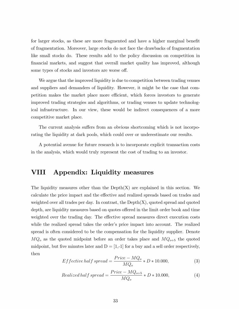
for larger stocks, as these are more fragmented and have a higher marginal bene�t

of fragmentation. Moreover, large stocks do not face the drawbacks of fragmentation

like small stocks do. These results add to the policy discussion on competition in

�nancial markets, and suggest that overall market quality has improved, although

some types of stocks and investors are worse o¤.

We argue that the improved liquidity is due to competition between trading venues

and suppliers and demanders of liquidity. However, it might be the case that com-

petition makes the market place more e¢ cient, which forces investors to generate

improved trading strategies and algorithms, or trading venues to update technolog-

ical infrastructure. In our view, these would be indirect consequences of a more

competitive market place.

The current analysis su¤ers from an obvious shortcoming which is not incorpo-

rating the liquidity at dark pools, which could over or underestimate our results.

A potential avenue for future research is to incorporate explicit transaction costs

in the analysis, which would truly represent the cost of trading to an investor.

VIII Appendix: Liquidity measures

The liquidity measures other than the Depth(X) are explained in this section. We

calculate the price impact and the e¤ective and realized spreads based on trades and

weighted over all trades per day. In contrast, the Depth(X), quoted spread and quoted

depth, are liquidity measures based on quotes o¤ered in the limit order book and time

weighted over the trading day. The e¤ective spread measures direct execution costs

while the realized spread takes the order�s price impact into account. The realized

spread is often considered to be the compensation for the liquidity supplier. Denote

MQo as the quoted midpoint before an order takes place and MQo+5 the quoted

midpoint, but �ve minutes later and D = [1,-1] for a buy and a sell order respectively,

then

Effective half spread =Price�MQo

MQo�D � 10:000; (3)

Realized half spread =Price�MQo+5

MQo�D � 10:000; (4)

33

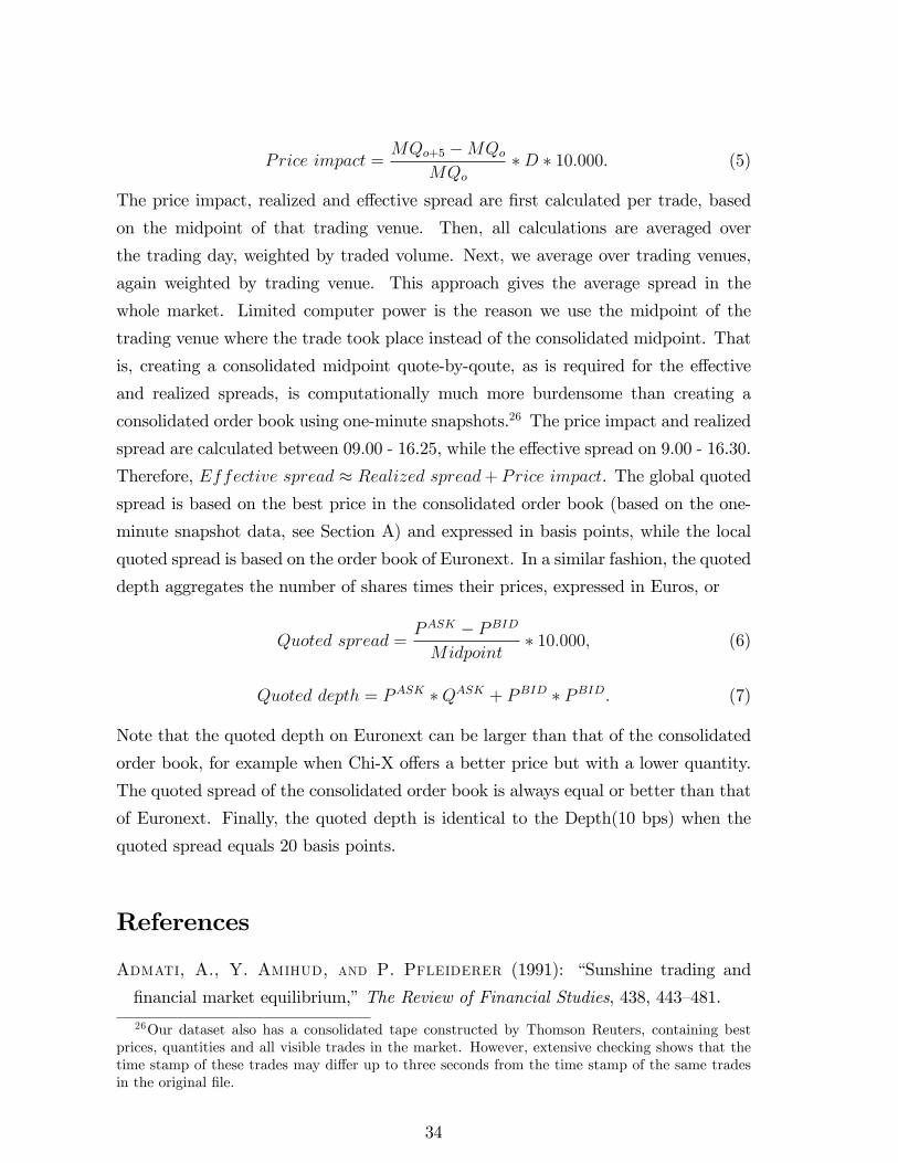
Price impact =MQo+5 �MQo

MQo�D � 10:000: (5)

The price impact, realized and e¤ective spread are �rst calculated per trade, based

on the midpoint of that trading venue. Then, all calculations are averaged over

the trading day, weighted by traded volume. Next, we average over trading venues,

again weighted by trading venue. This approach gives the average spread in the

whole market. Limited computer power is the reason we use the midpoint of the

trading venue where the trade took place instead of the consolidated midpoint. That

is, creating a consolidated midpoint quote-by-qoute, as is required for the e¤ective

and realized spreads, is computationally much more burdensome than creating a

consolidated order book using one-minute snapshots.26 The price impact and realized

spread are calculated between 09.00 - 16.25, while the e¤ective spread on 9.00 - 16.30.

Therefore, Effective spread � Realized spread+ Price impact. The global quotedspread is based on the best price in the consolidated order book (based on the one-

minute snapshot data, see Section A) and expressed in basis points, while the local

quoted spread is based on the order book of Euronext. In a similar fashion, the quoted

depth aggregates the number of shares times their prices, expressed in Euros, or

Quoted spread =PASK � PBIDMidpoint

� 10:000; (6)

Quoted depth = PASK �QASK + PBID � PBID: (7)

Note that the quoted depth on Euronext can be larger than that of the consolidated

order book, for example when Chi-X o¤ers a better price but with a lower quantity.

The quoted spread of the consolidated order book is always equal or better than that

of Euronext. Finally, the quoted depth is identical to the Depth(10 bps) when the

quoted spread equals 20 basis points.

References

Admati, A., Y. Amihud, and P. Pfleiderer (1991): �Sunshine trading and

�nancial market equilibrium,�The Review of Financial Studies, 438, 443�481.

26Our dataset also has a consolidated tape constructed by Thomson Reuters, containing bestprices, quantities and all visible trades in the market. However, extensive checking shows that thetime stamp of these trades may di¤er up to three seconds from the time stamp of the same tradesin the original �le.

34

Affleck-Graves, J., S. Hedge, and R. Miller (1994): �Trading Mechanisms

and the Components of the Bid-Ask Spread,�Journal of Finance, 49(4), 1471�1488.

Andersen, T., T. Bollerslev, F. Diebold, and H. Ebens (2001): �The dis-

tribution of realized stockreturn volatility,� Journal of Financial Economics, 61,

43�76.

Aubry, N., and M. McKee (2007): �MiFID: Where did It Come From, Where is

It Taking Us?,�Journal of International Banking Law and Regulation, 4, 177�186.

Barclay, M., T. Hendershott, and D. McCormick (2003): �Competition

among trading venues: Information and trading on electronic communications net-

works,�Journal of Finance, 58, 2637 �2666.

Battalio, R. (1997): �Third Market Broker-Dealers: Cost Competitors or Cream

Skimmers?,�Journal of Finance, 52(1), 341�352.

Bennett, P., and L. Wei (2006): �Market structure, fragmentation, and market

quality,�Journal of Financial Markets, 9(1), 49 �78.

Bessembinder, H., and H. Kaufman (1997): �A Comparison of Trade Execu-

tion Costs for NYSE and NASDAQ-Listed Stocks,�The Journal of Financial and

Quantitative Analysis, 32, 287�310.

Biais, B., C. Bisiere, and C. Spatt (2010): �Imperfect Competition in Financial

Markets: An Empirical Study of Island and Nasdaq,�Management Science, 56(12),

2237�2250.

Biais, B., D. Martimort, and J. Rochet (2000): �Competing Mechanisms in a

Common Value Environment,�Econometrica, 68(4), 799�837.

Boehmer, E. (2005): �Dimensions of execution quality: Recent evidence for US

equity markets,�Journal of Financial Economics, 78, 553�582.

Boehmer, E., G. Saar, and L. Yu (2005): �Lifting the Veil: An Analysis of

Pre-Trade Transparency at the NYSE,�Journal of Finance, 60, 783�815.

Cantillon, E., and P. Yin (2010): �Competition between Exchanges: A Research

Agenda,� forthcoming International Journal of Industrial Organization.

35

Chaboud, A., B. Chiquoine, E. Hjalmarsson, and C. Vega (2009): �Rise

of the machines: Algorithmic trading in the foreign exchange market,�Discussion

paper Federal Reserve System.

Chlistalla, M., and M. Lutat (2009): �The impact of new execution venues on

European equity markets liquidity: The case of Chi-X,�Proceedings of the Fifteenth

Americas Conference on Information Systems (AMCIS), San Francisco.

Chowdhry, B., and V. Nanda (1991): �Multimarket Trading and Market Liquid-

ity,�The Review of Financial Studies, 4(3), 483�511.

Conrad, J., K. Johnson, and S. Wahal (2003): �Institutional Trading and Al-

ternative Trading Systems,�Journal of Financial Economics, 70, 99�134.

Davies, R. (2008): �MiFID and a changing competitive landscape,�Working Paper

Series.

Davies, R., A. Dufour, and B. Scott-Quinn (2006): �The MiFID: Competi-

tion in a New European Equity Market Regulatory Structure,�Oxford Scholarship

Online Monographs, pp. 163�199.

Degryse, H., M. van Achter, and G. Wuyts (2010): �Internalization, Clearing

and Settlement and Market Liquidity,�EFA Frankfurt Paper.

Easley, D., N. Kiefer, and M. O�Hara (1996): �Cream-Skimming or Pro�t-

Sharing? The Curious Role of Purchased Order Flow,�The Journal of Finance,

51, 811�833.

Ende, B., P. Gomber, and M. Lutat (2010): �Smart order routing technology in

the New European Equity Trading Landscape,�Software Services for E-Business

and E-Society: 9th IFIP WG 6.1 Conference.

Ferrarini, G. A., and F. Recine (2006): Investor Protection In Europe: Corporate

Law Making, the MiFID and Beyond. Oxford University Press.

Foucault, T., O. Kadan, and E. Kandel (2009): �Liquidity Cycles and

Make/Take Fees in Electronic Markets,�EFA 2009 Bergen Meetings Paper.

Foucault, T., and A. Menkveld (2008): �Competition for order �ow and smart

order routing systems,�Journal of Finance, 63(1), 119�158.

36

Goldstein, M., and K. Kavajecz (2000): �Eights, sixteenths, and market depth:

changes in the tick size and liquidity provision on the NYSE,�Journal of Financial

Economics, 56, 125�149.

Gomber, P., and M. Gsell (2006): �Catching Up with Technology - The Im-

pact of Regulatory Changes on ECNs/MTFs and the Trading Venue Landscape in

Europe,�Competition and Regulation in Network Industries,, 1(4), 535�557.

Gomber, P., and A. Pierron (2010): �MiFID Spirit and Reality of a European

Financial Markets Directive,�Report Published by Celent.

Gomber, P., U. Schweickert, and E. Theissen (2004): �Zooming in on Liquid-

ity,�Working Paper Series.

Gresse, C. (2010): �Multi-Market Trading and Market Quality,�Working Paper.

Harris, L. (1993): �Consolidation, Fragmentation, Segmentation and Regulation.,�

Financial Markets, Institutions & Instruments, 5, 1�28.

Hasbrouck, J., and G. Saar (2009): �Technology and Liquidity Provision: The

Blurring of Traditional De�nitions,�Journal of Financial Markets, 12, 143�172.

Hendershott, T., C. Jones, and A. Menkveld (2010): �Does Algorithmic

Trading Improve Liquidity?,�Journal of Finance, forthcoming.

Hendershott, T., and R. Riordan (2009): �Algorithmic Trading and Informa-

tion,�Net Institute Working Paper 09-08.

Hengelbroc (2010): �Fourteen at one blow: The market entry of Turquoise,�Phd

dissertation - Bonn University.

Huang, R., and H. Stoll (2001): �Tick Size, Bid-Ask Spreads and Market Struc-

ture,�Journal of Financial and Quantitative Analysis, 36, 503�522.

O�Hara, M., and M. Ye (2009): �Is Market Fragmentation Harming Market Qual-

ity?,�Journal of Financial Economics, forthcoming.

Pagano, M. (1989a): �Endogenous Market Thinness and Stock Price Volatility,�

The Review of Economic Studies, 56, 269�287.

37

(1989b): �Trading volume and asset liquidity,�Quarterly Journal of Eco-

nomics, 104, 25�74.

Petrella, G. (2009): �MiFID, Reg NMS and Competition Across Trading Venues

in Europe and United States,�Working Paper.

Stoll, H. (2003): Market Microstructure. Handbook of the Economics of Finance.

(2006): �Electronic Trading in Stock Markets,�Journal of Economic Per-

spectives, 20(1), 153�174.

Weston, J. (2000): �Competition on the Nasdaq and the Impact of Recent Market

Reforms,�Journal of Finance, 55(6), 2565�2598.

(2002): �Electronic Communication Networks and Liquidity on the Nasdaq,�

Journal of Financial Services Research, 22, 125�139.

38

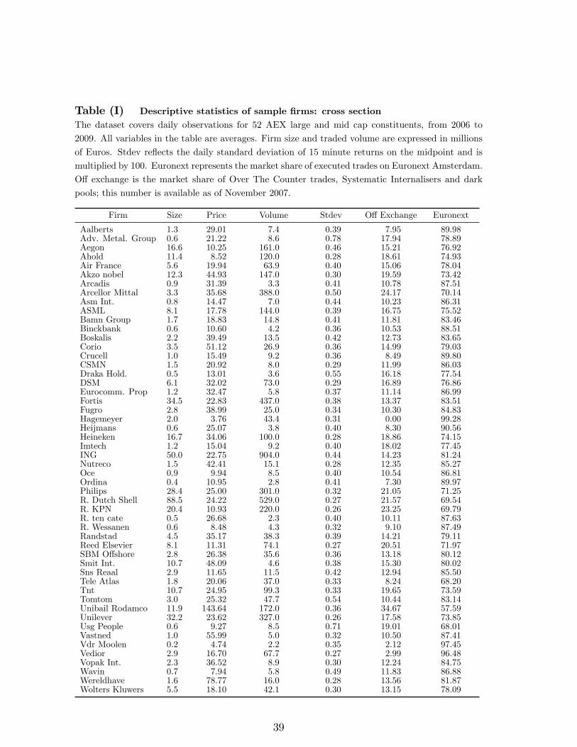
Table (I) Descriptive statistics of sample �rms: cross sectionThe dataset covers daily observations for 52 AEX large and mid cap constituents, from 2006 to

2009. All variables in the table are averages. Firm size and traded volume are expressed in millions

of Euros. Stdev re�ects the daily standard deviation of 15 minute returns on the midpoint and is

multiplied by 100. Euronext represents the market share of executed trades on Euronext Amsterdam.

O¤ exchange is the market share of Over The Counter trades, Systematic Internalisers and dark

pools; this number is available as of November 2007.

Firm Size Price Volume Stdev O¤ Exchange Euronext

Aalberts 1.3 29:01 7:4 0:39 7:95 89:98Adv. Metal. Group 0.6 21:22 8:6 0:78 17:94 78:89Aegon 16.6 10:25 161:0 0:46 15:21 76:92Ahold 11.4 8:52 120:0 0:28 18:61 74:93Air France 5.6 19:94 63:9 0:40 15:06 78:04Akzo nobel 12.3 44:93 147:0 0:30 19:59 73:42Arcadis 0.9 31:39 3:3 0:41 10:78 87:51Arcellor Mittal 3.3 35:68 388:0 0:50 24:17 70:14Asm Int. 0.8 14:47 7:0 0:44 10:23 86:31ASML 8.1 17:78 144:0 0:39 16:75 75:52Bamn Group 1.7 18:83 14:8 0:41 11:81 83:46Binckbank 0.6 10:60 4:2 0:36 10:53 88:51Boskalis 2.2 39:49 13:5 0:42 12:73 83:65Corio 3.5 51:12 26:9 0:36 14:99 79:03Crucell 1.0 15:49 9:2 0:36 8:49 89:80CSMN 1.5 20:92 8:0 0:29 11:99 86:03Draka Hold. 0.5 13:01 3:6 0:55 16:18 77:54DSM 6.1 32:02 73:0 0:29 16:89 76:86Eurocomm. Prop 1.2 32:47 5:8 0:37 11:14 86:99Fortis 34.5 22:83 437:0 0:38 13:37 83:51Fugro 2.8 38:99 25:0 0:34 10:30 84:83Hagemeyer 2.0 3:76 43:4 0:31 0:00 99:28Heijmans 0.6 25:07 3:8 0:40 8:30 90:56Heineken 16.7 34:06 100:0 0:28 18:86 74:15Imtech 1.2 15:04 9:2 0:40 18:02 77:45ING 50.0 22:75 904:0 0:44 14:23 81:24Nutreco 1.5 42:41 15:1 0:28 12:35 85:27Oce 0.9 9:94 8:5 0:40 10:54 86:81Ordina 0.4 10:95 2:8 0:41 7:30 89:97Philips 28.4 25:00 301:0 0:32 21:05 71:25R. Dutch Shell 88.5 24:22 529:0 0:27 21:57 69:54R. KPN 20.4 10:93 220:0 0:26 23:25 69:79R. ten cate 0.5 26:68 2:3 0:40 10:11 87:63R. Wessanen 0.6 8:48 4:3 0:32 9:10 87:49Randstad 4.5 35:17 38:3 0:39 14:21 79:11Reed Elsevier 8.1 11:31 74:1 0:27 20:51 71:97SBM O¤shore 2.8 26:38 35:6 0:36 13:18 80:12Smit Int. 10.7 48:09 4:6 0:38 15:30 80:02Sns Reaal 2.9 11:65 11:5 0:42 12:94 85:50Tele Atlas 1.8 20:06 37:0 0:33 8:24 68:20Tnt 10.7 24:95 99:3 0:33 19:65 73:59Tomtom 3.0 25:32 47:7 0:54 10:44 83:14Unibail Rodamco 11.9 143:64 172:0 0:36 34:67 57:59Unilever 32.2 23:62 327:0 0:26 17:58 73:85Usg People 0.6 9:27 8:5 0:71 19:01 68:01Vastned 1.0 55:99 5:0 0:32 10:50 87:41Vdr Moolen 0.2 4:74 2:2 0:35 2:12 97:45Vedior 2.9 16:70 67:7 0:27 2:99 96:48Vopak Int. 2.3 36:52 8:9 0:30 12:24 84:75Wavin 0.7 7:94 5:8 0:49 11:83 86:88Wereldhave 1.6 78:77 16:0 0:28 13:56 81:87Wolters Kluwers 5.5 18:10 42:1 0:30 13:15 78:09

39

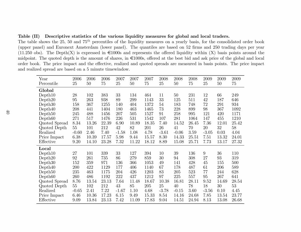
Table (II) Descriptive statistics of the various liquidity measures for global and local traders.The table shows the 25, 50 and 75th percentiles of the liquidity measures on a yearly basis, for the consolidated order book(upper panel) and Euronext Amsterdam (lower panel). The quantiles are based on 52 �rms and 250 trading days per year(11.250 obs). The Depth(X) is expressed in e1000s and represents the o¤ered liquidity within (X) basis points around themidpoint. The quoted depth is the amount of shares, in e1000s, o¤ered at the best bid and ask price of the global and localorder book. The price impact and the e¤ective, realized and quoted spreads are measured in basis points. The price impactand realized spread are based on a 5 minute timewindow.

Year 2006 2006 2006 2007 2007 2007 2008 2008 2008 2009 2009 2009Percentile 25 50 75 25 50 75 25 50 75 25 50 75

GlobalDepth10 28 102 383 33 134 464 11 50 231 12 66 249Depth20 95 263 938 89 299 1143 33 125 511 42 187 646Depth30 158 367 1255 140 404 1372 54 183 748 72 291 934Depth40 208 441 1404 180 463 1465 73 228 899 98 367 1092Depth50 245 488 1456 207 505 1527 91 258 995 121 420 1171Depth60 271 517 1476 226 531 1542 107 281 1064 147 455 1210Quoted Spread 8.34 13.26 22.39 6.90 10.89 18.35 7.40 14.52 26.45 7.36 12.01 25.42Quoted Depth 55 101 212 42 82 201 26 41 70 20 32 58Realized -0.60 2.46 7.40 -1.58 1.08 4.78 -3.61 -0.06 3.59 -3.05 0.03 4.04Price Impact 6.38 10.39 17.57 5.98 9.44 15.57 8.30 14.33 25.51 7.51 13.32 24.01E¤ective 9.20 14.10 23.28 7.32 11.22 18.12 8.89 15.08 25.71 7.73 13.17 27.32

LocalDepth10 27 101 339 33 127 394 10 39 136 9 36 110Depth20 92 261 735 86 279 859 30 94 308 27 93 319Depth30 152 359 971 136 366 1053 49 141 428 45 155 500Depth40 200 422 1129 177 406 1140 67 178 487 61 206 589Depth50 235 463 1175 204 426 1203 83 205 523 77 244 628Depth60 260 486 1192 222 437 1212 97 225 557 95 267 641Quoted Spread 8.76 13.54 23.13 7.64 11.48 18.67 10.38 16.81 28.11 9.52 14.69 28.54Quoted Depth 55 102 212 43 85 205 25 40 78 18 30 53Realized -0.65 2.41 7.22 -1.67 1.10 4.68 -3.78 -0.15 3.60 -3.56 0.10 4.45Price Impact 6.46 10.36 17.23 6.15 9.49 15.33 8.54 14.16 24.68 7.85 13.54 23.77E¤ective 9.09 13.84 23.13 7.42 11.09 17.83 9.04 14.51 24.94 8.13 13.08 26.68

40

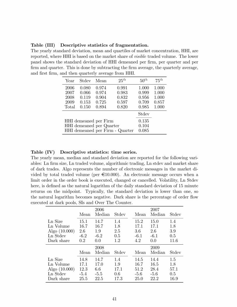
Table (III) Descriptive statistics of fragmentation.The yearly standard deviation, mean and quartiles of market concentration, HHI, arereported, where HHI is based on the market share of visible traded volume. The lowerpanel shows the standard deviation of HHI demeaned per �rm, per quarter and per�rm and quarter. This is done by subtracting the �rm average, the quarterly average,and �rst �rm, and then quarterly average from HHI.

Year Stdev Mean 25th 50th 75th

2006 0.080 0.974 0.991 1.000 1.0002007 0.066 0.974 0.983 0.999 1.0002008 0.119 0.904 0.832 0.956 1.0002009 0.153 0.725 0.597 0.709 0.857Total 0.150 0.894 0.820 0.985 1.000

Stdev

HHI demeaned per Firm 0.135HHI demeaned per Quarter 0.104HHI demeaned per Firm - Quarter 0.085

Table (IV) Descriptive statistics: time series.The yearly mean, median and standard deviation are reported for the following vari-ables: Ln �rm size, Ln traded volume, algorithmic trading, Ln stdev and market shareof dark trades. Algo represents the number of electronic messages in the market di-vided by total traded volume (per e10.000). An electronic message occurs when alimit order in the order book is executed, changed or cancelled. Volatility, Ln Stdevhere, is de�ned as the natural logarithm of the daily standard deviation of 15 minutereturns on the midpoint. Typically, the standard deviation is lower than one, sothe natural logarithm becomes negative. Dark share is the percentage of order �owexecuted at dark pools, SIs and Over The Counter.

2006 2007Mean Median Stdev Mean Median Stdev

Ln Size 15.1 14.7 1.4 15.2 15.0 1.4Ln Volume 16.7 16.7 1.8 17.1 17.1 1.8Algo (10.000) 2.6 1.9 2.5 3.6 2.6 3.9Ln Stdev -6.2 -6.2 0.5 -6.1 -6.1 0.5Dark share 0.2 0.0 1.2 4.2 0.0 11.6

2008 2009Mean Median Stdev Mean Median Stdev

Ln Size 14.8 14.7 1.4 14.5 14.4 1.5Ln Volume 17.1 17.0 1.9 16.7 16.5 1.8Algo (10.000) 12.3 6.6 17.1 51.2 28.4 57.1Ln Stdev -5.4 -5.5 0.6 -5.6 -5.6 0.5Dark share 25.5 22.5 17.3 25.0 22.2 16.9

41

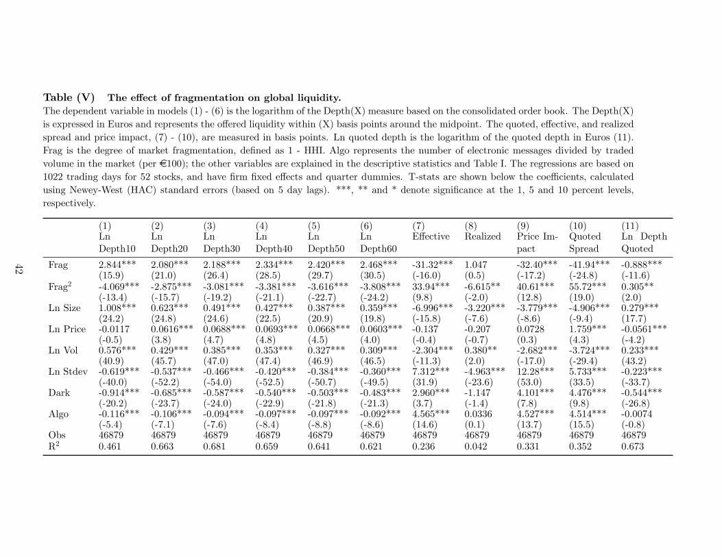
Table (V) The e¤ect of fragmentation on global liquidity.The dependent variable in models (1) - (6) is the logarithm of the Depth(X) measure based on the consolidated order book. The Depth(X)is expressed in Euros and represents the o¤ered liquidity within (X) basis points around the midpoint. The quoted, e¤ective, and realizedspread and price impact, (7) - (10), are measured in basis points. Ln quoted depth is the logarithm of the quoted depth in Euros (11).Frag is the degree of market fragmentation, de�ned as 1 - HHI. Algo represents the number of electronic messages divided by tradedvolume in the market (per e100); the other variables are explained in the descriptive statistics and Table I. The regressions are based on1022 trading days for 52 stocks, and have �rm �xed e¤ects and quarter dummies. T-stats are shown below the coe¢ cients, calculatedusing Newey-West (HAC) standard errors (based on 5 day lags). ***, ** and * denote signi�cance at the 1, 5 and 10 percent levels,respectively.

(1) (2) (3) (4) (5) (6) (7) (8) (9) (10) (11)LnDepth10

LnDepth20

LnDepth30

LnDepth40

LnDepth50

LnDepth60

E¤ective Realized Price Im-pact

QuotedSpread

Ln DepthQuoted

Frag 2.844*** 2.080*** 2.188*** 2.334*** 2.420*** 2.468*** -31.32*** 1.047 -32.40*** -41.94*** -0.888***(15.9) (21.0) (26.4) (28.5) (29.7) (30.5) (-16.0) (0.5) (-17.2) (-24.8) (-11.6)

Frag2 -4.069*** -2.875*** -3.081*** -3.381*** -3.616*** -3.808*** 33.94*** -6.615** 40.61*** 55.72*** 0.305**(-13.4) (-15.7) (-19.2) (-21.1) (-22.7) (-24.2) (9.8) (-2.0) (12.8) (19.0) (2.0)

Ln Size 1.008*** 0.623*** 0.491*** 0.427*** 0.387*** 0.359*** -6.996*** -3.220*** -3.779*** -4.906*** 0.279***(24.2) (24.8) (24.6) (22.5) (20.9) (19.8) (-15.8) (-7.6) (-8.6) (-9.4) (17.7)

Ln Price -0.0117 0.0616*** 0.0688*** 0.0693*** 0.0668*** 0.0603*** -0.137 -0.207 0.0728 1.759*** -0.0561***(-0.5) (3.8) (4.7) (4.8) (4.5) (4.0) (-0.4) (-0.7) (0.3) (4.3) (-4.2)

Ln Vol 0.576*** 0.429*** 0.385*** 0.353*** 0.327*** 0.309*** -2.304*** 0.380** -2.682*** -3.724*** 0.233***(40.9) (45.7) (47.0) (47.4) (46.9) (46.5) (-11.3) (2.0) (-17.0) (-29.4) (43.2)

Ln Stdev -0.619*** -0.537*** -0.466*** -0.420*** -0.384*** -0.360*** 7.312*** -4.963*** 12.28*** 5.733*** -0.223***(-40.0) (-52.2) (-54.0) (-52.5) (-50.7) (-49.5) (31.9) (-23.6) (53.0) (33.5) (-33.7)

Dark -0.914*** -0.685*** -0.587*** -0.540*** -0.503*** -0.483*** 2.960*** -1.147 4.101*** 4.476*** -0.544***(-20.2) (-23.7) (-24.0) (-22.9) (-21.8) (-21.3) (3.7) (-1.4) (7.8) (9.8) (-26.8)

Algo -0.116*** -0.106*** -0.094*** -0.097*** -0.097*** -0.092*** 4.565*** 0.0336 4.527*** 4.514*** -0.0074(-5.4) (-7.1) (-7.6) (-8.4) (-8.8) (-8.6) (14.6) (0.1) (13.7) (15.5) (-0.8)

Obs 46879 46879 46879 46879 46879 46879 46879 46879 46879 46879 46879R2 0.461 0.663 0.681 0.659 0.641 0.621 0.236 0.042 0.331 0.352 0.673

42

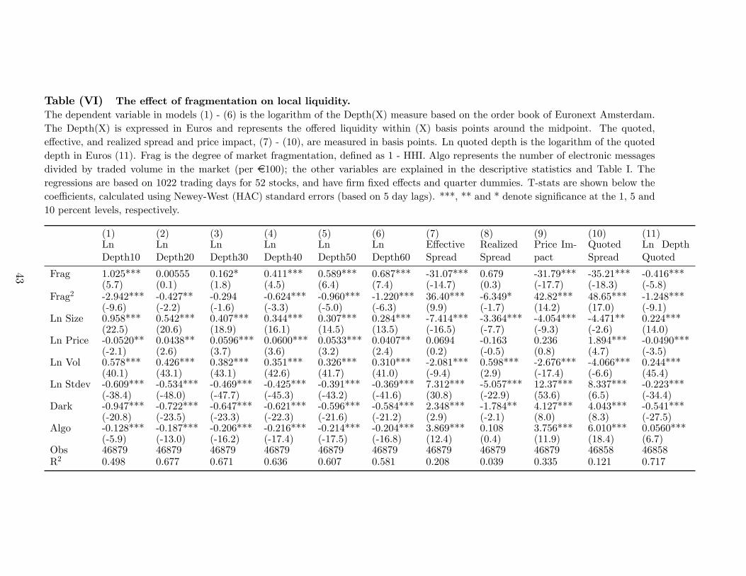
Table (VI) The e¤ect of fragmentation on local liquidity.The dependent variable in models (1) - (6) is the logarithm of the Depth(X) measure based on the order book of Euronext Amsterdam.The Depth(X) is expressed in Euros and represents the o¤ered liquidity within (X) basis points around the midpoint. The quoted,e¤ective, and realized spread and price impact, (7) - (10), are measured in basis points. Ln quoted depth is the logarithm of the quoteddepth in Euros (11). Frag is the degree of market fragmentation, de�ned as 1 - HHI. Algo represents the number of electronic messagesdivided by traded volume in the market (per e100); the other variables are explained in the descriptive statistics and Table I. Theregressions are based on 1022 trading days for 52 stocks, and have �rm �xed e¤ects and quarter dummies. T-stats are shown below thecoe¢ cients, calculated using Newey-West (HAC) standard errors (based on 5 day lags). ***, ** and * denote signi�cance at the 1, 5 and10 percent levels, respectively.

(1) (2) (3) (4) (5) (6) (7) (8) (9) (10) (11)LnDepth10

LnDepth20

LnDepth30

LnDepth40

LnDepth50

LnDepth60

E¤ectiveSpread

RealizedSpread

Price Im-pact

QuotedSpread

Ln DepthQuoted

Frag 1.025*** 0.00555 0.162* 0.411*** 0.589*** 0.687*** -31.07*** 0.679 -31.79*** -35.21*** -0.416***(5.7) (0.1) (1.8) (4.5) (6.4) (7.4) (-14.7) (0.3) (-17.7) (-18.3) (-5.8)

Frag2 -2.942*** -0.427** -0.294 -0.624*** -0.960*** -1.220*** 36.40*** -6.349* 42.82*** 48.65*** -1.248***(-9.6) (-2.2) (-1.6) (-3.3) (-5.0) (-6.3) (9.9) (-1.7) (14.2) (17.0) (-9.1)

Ln Size 0.958*** 0.542*** 0.407*** 0.344*** 0.307*** 0.284*** -7.414*** -3.364*** -4.054*** -4.471** 0.224***(22.5) (20.6) (18.9) (16.1) (14.5) (13.5) (-16.5) (-7.7) (-9.3) (-2.6) (14.0)

Ln Price -0.0520** 0.0438** 0.0596*** 0.0600*** 0.0533*** 0.0407** 0.0694 -0.163 0.236 1.894*** -0.0490***(-2.1) (2.6) (3.7) (3.6) (3.2) (2.4) (0.2) (-0.5) (0.8) (4.7) (-3.5)

Ln Vol 0.578*** 0.426*** 0.382*** 0.351*** 0.326*** 0.310*** -2.081*** 0.598*** -2.676*** -4.066*** 0.244***(40.1) (43.1) (43.1) (42.6) (41.7) (41.0) (-9.4) (2.9) (-17.4) (-6.6) (45.4)

Ln Stdev -0.609*** -0.534*** -0.469*** -0.425*** -0.391*** -0.369*** 7.312*** -5.057*** 12.37*** 8.337*** -0.223***(-38.4) (-48.0) (-47.7) (-45.3) (-43.2) (-41.6) (30.8) (-22.9) (53.6) (6.5) (-34.4)

Dark -0.947*** -0.722*** -0.647*** -0.621*** -0.596*** -0.584*** 2.348*** -1.784** 4.127*** 4.043*** -0.541***(-20.8) (-23.5) (-23.3) (-22.3) (-21.6) (-21.2) (2.9) (-2.1) (8.0) (8.3) (-27.5)

Algo -0.128*** -0.187*** -0.206*** -0.216*** -0.214*** -0.204*** 3.869*** 0.108 3.756*** 6.010*** 0.0560***(-5.9) (-13.0) (-16.2) (-17.4) (-17.5) (-16.8) (12.4) (0.4) (11.9) (18.4) (6.7)

Obs 46879 46879 46879 46879 46879 46879 46879 46879 46879 46858 46858R2 0.498 0.677 0.671 0.636 0.607 0.581 0.208 0.039 0.335 0.121 0.717

43

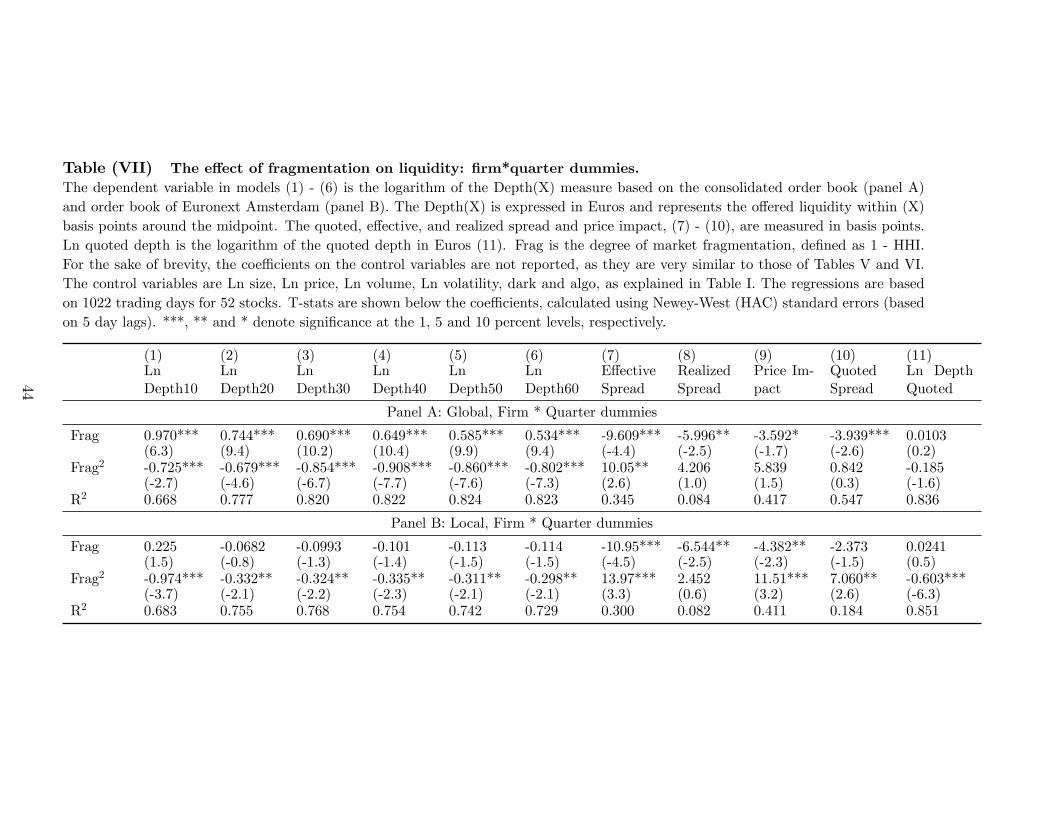
Table (VII) The e¤ect of fragmentation on liquidity: �rm*quarter dummies.The dependent variable in models (1) - (6) is the logarithm of the Depth(X) measure based on the consolidated order book (panel A)and order book of Euronext Amsterdam (panel B). The Depth(X) is expressed in Euros and represents the o¤ered liquidity within (X)basis points around the midpoint. The quoted, e¤ective, and realized spread and price impact, (7) - (10), are measured in basis points.Ln quoted depth is the logarithm of the quoted depth in Euros (11). Frag is the degree of market fragmentation, de�ned as 1 - HHI.For the sake of brevity, the coe¢ cients on the control variables are not reported, as they are very similar to those of Tables V and VI.The control variables are Ln size, Ln price, Ln volume, Ln volatility, dark and algo, as explained in Table I. The regressions are basedon 1022 trading days for 52 stocks. T-stats are shown below the coe¢ cients, calculated using Newey-West (HAC) standard errors (basedon 5 day lags). ***, ** and * denote signi�cance at the 1, 5 and 10 percent levels, respectively.

(1) (2) (3) (4) (5) (6) (7) (8) (9) (10) (11)LnDepth10

LnDepth20

LnDepth30

LnDepth40

LnDepth50

LnDepth60

E¤ectiveSpread

RealizedSpread

Price Im-pact

QuotedSpread

Ln DepthQuoted

Panel A: Global, Firm * Quarter dummies

Frag 0.970*** 0.744*** 0.690*** 0.649*** 0.585*** 0.534*** -9.609*** -5.996** -3.592* -3.939*** 0.0103(6.3) (9.4) (10.2) (10.4) (9.9) (9.4) (-4.4) (-2.5) (-1.7) (-2.6) (0.2)

Frag2 -0.725*** -0.679*** -0.854*** -0.908*** -0.860*** -0.802*** 10.05** 4.206 5.839 0.842 -0.185(-2.7) (-4.6) (-6.7) (-7.7) (-7.6) (-7.3) (2.6) (1.0) (1.5) (0.3) (-1.6)

R2 0.668 0.777 0.820 0.822 0.824 0.823 0.345 0.084 0.417 0.547 0.836

Panel B: Local, Firm * Quarter dummies

Frag 0.225 -0.0682 -0.0993 -0.101 -0.113 -0.114 -10.95*** -6.544** -4.382** -2.373 0.0241(1.5) (-0.8) (-1.3) (-1.4) (-1.5) (-1.5) (-4.5) (-2.5) (-2.3) (-1.5) (0.5)

Frag2 -0.974*** -0.332** -0.324** -0.335** -0.311** -0.298** 13.97*** 2.452 11.51*** 7.060** -0.603***(-3.7) (-2.1) (-2.2) (-2.3) (-2.1) (-2.1) (3.3) (0.6) (3.2) (2.6) (-6.3)

R2 0.683 0.755 0.768 0.754 0.742 0.729 0.300 0.082 0.411 0.184 0.851

44

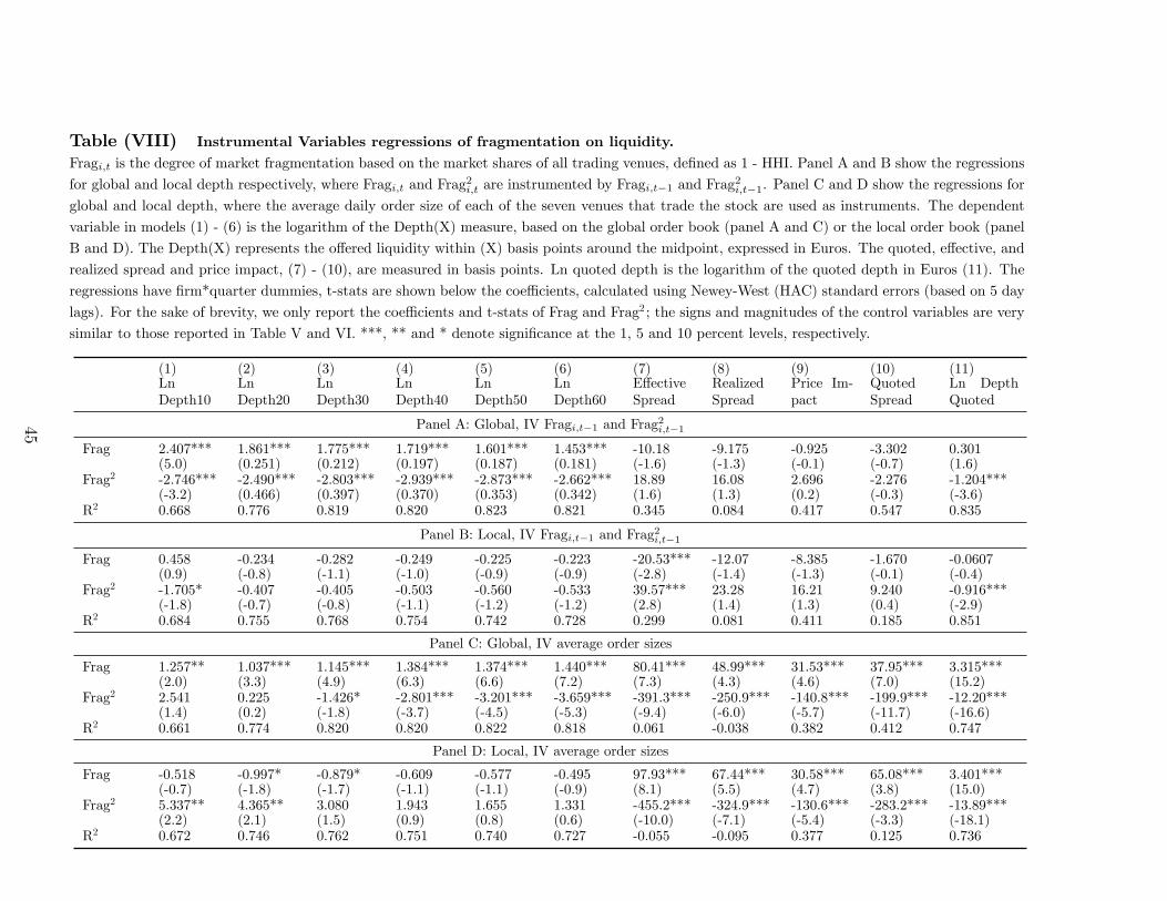
Table (VIII) Instrumental Variables regressions of fragmentation on liquidity.Fragi;t is the degree of market fragmentation based on the market shares of all trading venues, de�ned as 1 - HHI. Panel A and B show the regressions

for global and local depth respectively, where Fragi;t and Frag2i;t are instrumented by Fragi;t�1 and Frag2i;t�1. Panel C and D show the regressions for

global and local depth, where the average daily order size of each of the seven venues that trade the stock are used as instruments. The dependent

variable in models (1) - (6) is the logarithm of the Depth(X) measure, based on the global order book (panel A and C) or the local order book (panel

B and D). The Depth(X) represents the o¤ered liquidity within (X) basis points around the midpoint, expressed in Euros. The quoted, e¤ective, and

realized spread and price impact, (7) - (10), are measured in basis points. Ln quoted depth is the logarithm of the quoted depth in Euros (11). The

regressions have �rm*quarter dummies, t-stats are shown below the coe¢ cients, calculated using Newey-West (HAC) standard errors (based on 5 day

lags). For the sake of brevity, we only report the coe¢ cients and t-stats of Frag and Frag2 ; the signs and magnitudes of the control variables are very

similar to those reported in Table V and VI. ***, ** and * denote signi�cance at the 1, 5 and 10 percent levels, respectively.

(1) (2) (3) (4) (5) (6) (7) (8) (9) (10) (11)LnDepth10

LnDepth20

LnDepth30

LnDepth40

LnDepth50

LnDepth60

E¤ectiveSpread

RealizedSpread

Price Im-pact

QuotedSpread

Ln DepthQuoted

Panel A: Global, IV Fragi;t�1 and Frag2i;t�1

Frag 2.407*** 1.861*** 1.775*** 1.719*** 1.601*** 1.453*** -10.18 -9.175 -0.925 -3.302 0.301(5.0) (0.251) (0.212) (0.197) (0.187) (0.181) (-1.6) (-1.3) (-0.1) (-0.7) (1.6)

Frag2 -2.746*** -2.490*** -2.803*** -2.939*** -2.873*** -2.662*** 18.89 16.08 2.696 -2.276 -1.204***(-3.2) (0.466) (0.397) (0.370) (0.353) (0.342) (1.6) (1.3) (0.2) (-0.3) (-3.6)

R2 0.668 0.776 0.819 0.820 0.823 0.821 0.345 0.084 0.417 0.547 0.835

Panel B: Local, IV Fragi;t�1 and Frag2i;t�1

Frag 0.458 -0.234 -0.282 -0.249 -0.225 -0.223 -20.53*** -12.07 -8.385 -1.670 -0.0607(0.9) (-0.8) (-1.1) (-1.0) (-0.9) (-0.9) (-2.8) (-1.4) (-1.3) (-0.1) (-0.4)

Frag2 -1.705* -0.407 -0.405 -0.503 -0.560 -0.533 39.57*** 23.28 16.21 9.240 -0.916***(-1.8) (-0.7) (-0.8) (-1.1) (-1.2) (-1.2) (2.8) (1.4) (1.3) (0.4) (-2.9)

R2 0.684 0.755 0.768 0.754 0.742 0.728 0.299 0.081 0.411 0.185 0.851

Panel C: Global, IV average order sizes

Frag 1.257** 1.037*** 1.145*** 1.384*** 1.374*** 1.440*** 80.41*** 48.99*** 31.53*** 37.95*** 3.315***(2.0) (3.3) (4.9) (6.3) (6.6) (7.2) (7.3) (4.3) (4.6) (7.0) (15.2)

Frag2 2.541 0.225 -1.426* -2.801*** -3.201*** -3.659*** -391.3*** -250.9*** -140.8*** -199.9*** -12.20***(1.4) (0.2) (-1.8) (-3.7) (-4.5) (-5.3) (-9.4) (-6.0) (-5.7) (-11.7) (-16.6)

R2 0.661 0.774 0.820 0.820 0.822 0.818 0.061 -0.038 0.382 0.412 0.747

Panel D: Local, IV average order sizes

Frag -0.518 -0.997* -0.879* -0.609 -0.577 -0.495 97.93*** 67.44*** 30.58*** 65.08*** 3.401***(-0.7) (-1.8) (-1.7) (-1.1) (-1.1) (-0.9) (8.1) (5.5) (4.7) (3.8) (15.0)

Frag2 5.337** 4.365** 3.080 1.943 1.655 1.331 -455.2*** -324.9*** -130.6*** -283.2*** -13.89***(2.2) (2.1) (1.5) (0.9) (0.8) (0.6) (-10.0) (-7.1) (-5.4) (-3.3) (-18.1)

R2 0.672 0.746 0.762 0.751 0.740 0.727 -0.055 -0.095 0.377 0.125 0.736

45

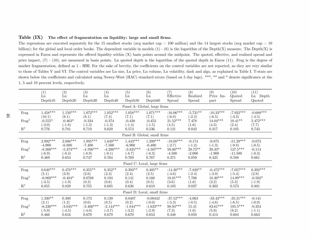
Table (IX) The e¤ect of fragmentation on liquidity: large and small �rms.The regressions are executed separately for the 15 smallest stocks (avg market cap < 100 million) and the 14 largest stocks (avg market cap > 10

billion); for the global and local order books. The dependent variable in models (1) - (6) is the logarithm of the Depth(X) measure. The Depth(X) is

expressed in Euros and represents the o¤ered liquidity within (X) basis points around the midpoint. The quoted, e¤ective, and realized spread and

price impact, (7) - (10), are measured in basis points. Ln quoted depth is the logarithm of the quoted depth in Euros (11). Frag is the degree of

market fragmentation, de�ned as 1 - HHI. For the sake of brevity, the coe¢ cients on the control variables are not reported, as they are very similar

to those of Tables V and VI. The control variables are Ln size, Ln price, Ln volume, Ln volatility, dark and algo, as explained in Table I. T-stats are

shown below the coe¢ cients and calculated using Newey-West (HAC) standard errors (based on 5 day lags). ***, ** and * denote signi�cance at the

1, 5 and 10 percent levels, respectively.

(1) (2) (3) (4) (5) (6) (7) (8) (9) (10) (11)LnDepth10

LnDepth20

LnDepth30

LnDepth40

LnDepth50

LnDepth60

E¤ectiveSpread

RealizedSpread

Price Im-pact

QuotedSpread

Ln DepthQuoted

Panel A: Global, large �rms

Frag 1.458*** 1.150*** 1.072*** 1.052*** 1.058*** 1.071*** -16.06*** -5.731** -10.33*** -7.922*** -0.688***(10.1) (9.1) (8.1) (7.4) (7.1) (7.1) (-6.0) (-2.2) (-6.5) (-3.3) (-4.5)

Frag2 -0.555* -0.463* -0.334 -0.374 -0.438 -0.452 21.52*** 7.478 14.04*** 10.41** 2.472***(-2.0) (-1.8) (-1.2) (-1.3) (-1.4) (-1.5) (4.5) (1.6) (4.3) (2.4) (7.7)

R2 0.776 0.781 0.710 0.629 0.574 0.536 0.121 0.042 0.317 0.105 0.743

Panel B: Global, small �rms

Frag 2.992*** 2.086*** 1.805*** 1.649*** 1.443*** 1.299*** -19.08*** -9.174 -9.875 -51.29*** -0.073-4.900 -6.800 -7.400 -7.500 -6.900 -6.400 (-2.7) (-1.2) (-1.3) (-9.8) (-0.5)

Frag2 -8.300*** -5.373*** -4.706*** -4.290*** -3.825*** -3.507*** 59.00*** 29.72** 29.33* 127.5*** -0.114(-6.9) (-8.4) (-8.9) (-9.1) (-8.7) (-8.3) -4.500 -2.000 -1.900 -11.500 (-0.3)

R2 0.469 0.654 0.747 0.764 0.769 0.767 0.371 0.059 0.425 0.588 0.661

Panel C: Local, large �rms

Frag 0.640*** 0.478*** 0.355** 0.352** 0.393** 0.405** -14.30*** -7.828** -6.472*** -7.057*** 0.392***(5.1) (3.9) (2.6) (2.3) (2.4) (2.5) (-4.6) (-2.4) (-3.9) (-5.4) (2.9)

Frag2 -0.869*** -0.484* 0.0768 0.194 0.141 0.166 18.01*** 7.706 10.30*** 14.99*** -0.502*(-3.5) (-1.9) (0.3) (0.6) (0.4) (0.5) (3.6) (1.6) (3.2) (5.3) (-1.9)

R2 0.855 0.829 0.755 0.685 0.638 0.610 0.105 0.037 0.303 0.573 0.801

Panel D: Local, small �rms

Frag 1.330** 0.380 0.173 0.139 0.0487 -0.00442 -37.52*** -4.063 -33.43*** -35.21*** -0.141(2.1) (1.2) (0.6) (0.5) (0.2) (-0.0) (-5.3) (-0.5) (-4.6) (-6.5) (-0.9)

Frag2 -6.230*** -3.045*** -2.406*** -2.144*** -1.844*** -1.633*** 98.94*** 15.41 83.61*** 105.5*** -0.354(-5.0) (-4.5) (-4.0) (-3.7) (-3.2) (-2.9) (7.3) (1.0) (5.9) (9.2) (-1.1)

R2 0.466 0.616 0.679 0.679 0.670 0.653 0.348 0.058 0.414 0.604 0.663

46

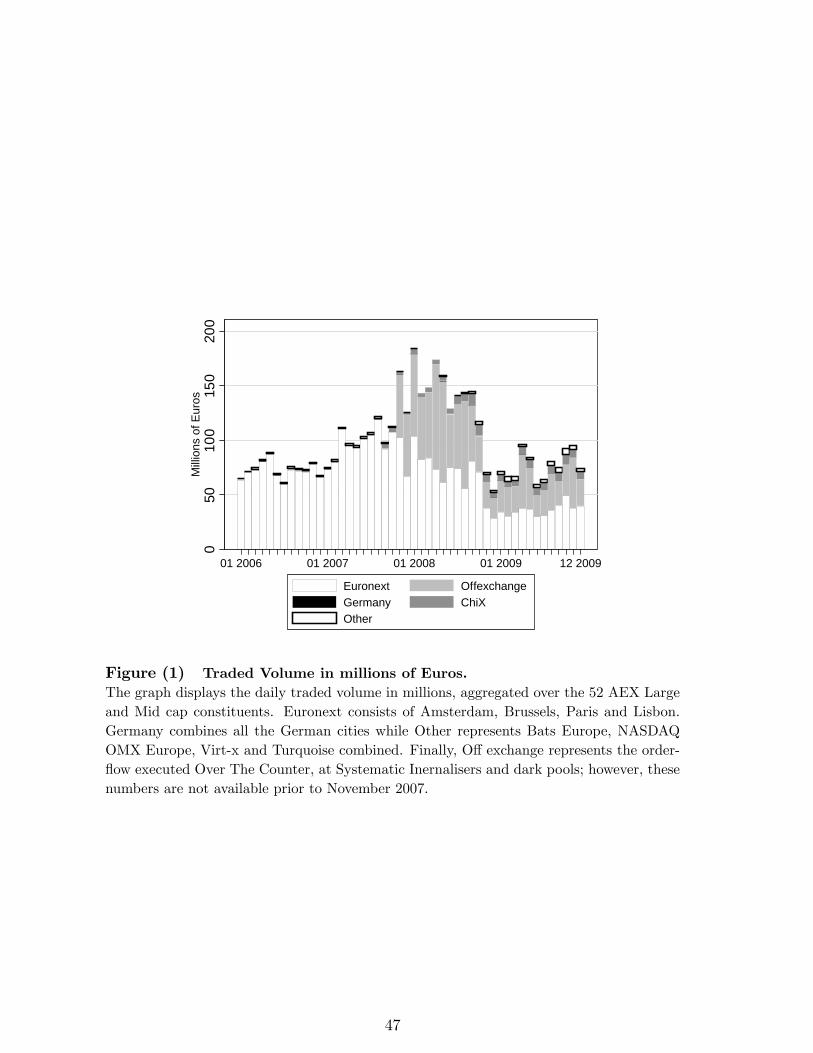
050

100

150

200

Milli

ons 

of E

uros

01 2006 01 2007 01 2008 01 2009 12 2009

Euronext OffexchangeGermany ChiXOther

Figure (1) Traded Volume in millions of Euros.The graph displays the daily traded volume in millions, aggregated over the 52 AEX Largeand Mid cap constituents. Euronext consists of Amsterdam, Brussels, Paris and Lisbon.Germany combines all the German cities while Other represents Bats Europe, NASDAQOMX Europe, Virt-x and Turquoise combined. Finally, O¤ exchange represents the order-�ow executed Over The Counter, at Systematic Inernalisers and dark pools; however, thesenumbers are not available prior to November 2007.

47

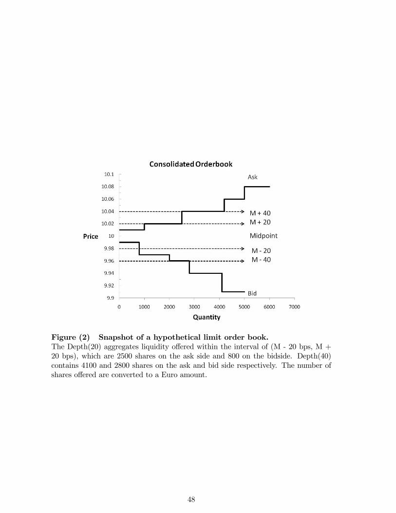
Figure (2) Snapshot of a hypothetical limit order book.The Depth(20) aggregates liquidity o¤ered within the interval of (M - 20 bps, M +20 bps), which are 2500 shares on the ask side and 800 on the bidside. Depth(40)contains 4100 and 2800 shares on the ask and bid side respectively. The number ofshares o¤ered are converted to a Euro amount.

48

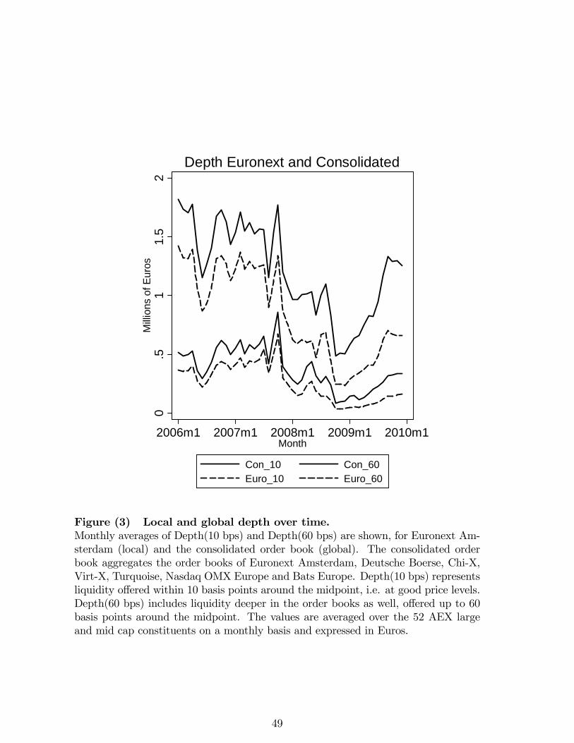
0.5

11.

52

Milli

ons 

of E

uros

2006m1 2007m1 2008m1 2009m1 2010m1Month

Con_10 Con_60Euro_10 Euro_60

Depth Euronext and Consolidated

Figure (3) Local and global depth over time.Monthly averages of Depth(10 bps) and Depth(60 bps) are shown, for Euronext Am-sterdam (local) and the consolidated order book (global). The consolidated orderbook aggregates the order books of Euronext Amsterdam, Deutsche Boerse, Chi-X,Virt-X, Turquoise, Nasdaq OMX Europe and Bats Europe. Depth(10 bps) representsliquidity o¤ered within 10 basis points around the midpoint, i.e. at good price levels.Depth(60 bps) includes liquidity deeper in the order books as well, o¤ered up to 60basis points around the midpoint. The values are averaged over the 52 AEX largeand mid cap constituents on a monthly basis and expressed in Euros.

49

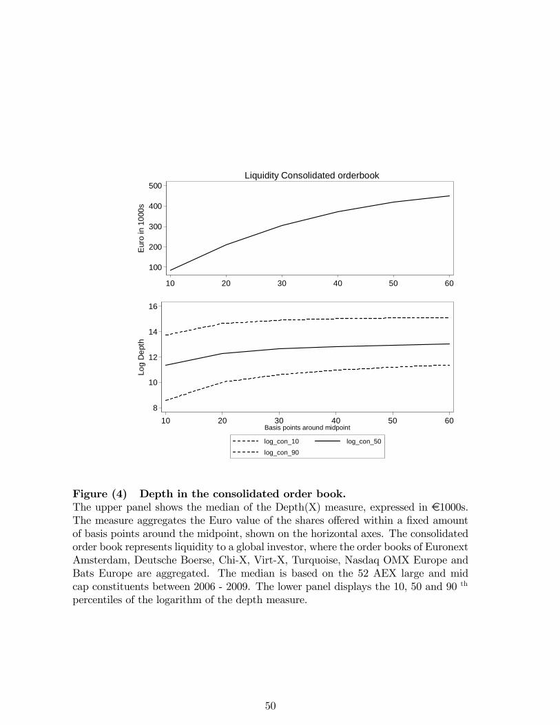
100

200

300

400

500

Eur

o in

 100

0s

10 20 30 40 50 60

Liquidity Consolidated orderbook

8

10

12

14

16

Log 

Dep

th

10 20 30 40 50 60Basis points around midpoint

log_con_10 log_con_50

log_con_90

Figure (4) Depth in the consolidated order book.The upper panel shows the median of the Depth(X) measure, expressed in e1000s.The measure aggregates the Euro value of the shares o¤ered within a �xed amountof basis points around the midpoint, shown on the horizontal axes. The consolidatedorder book represents liquidity to a global investor, where the order books of EuronextAmsterdam, Deutsche Boerse, Chi-X, Virt-X, Turquoise, Nasdaq OMX Europe andBats Europe are aggregated. The median is based on the 52 AEX large and midcap constituents between 2006 - 2009. The lower panel displays the 10, 50 and 90 th

percentiles of the logarithm of the depth measure.

50

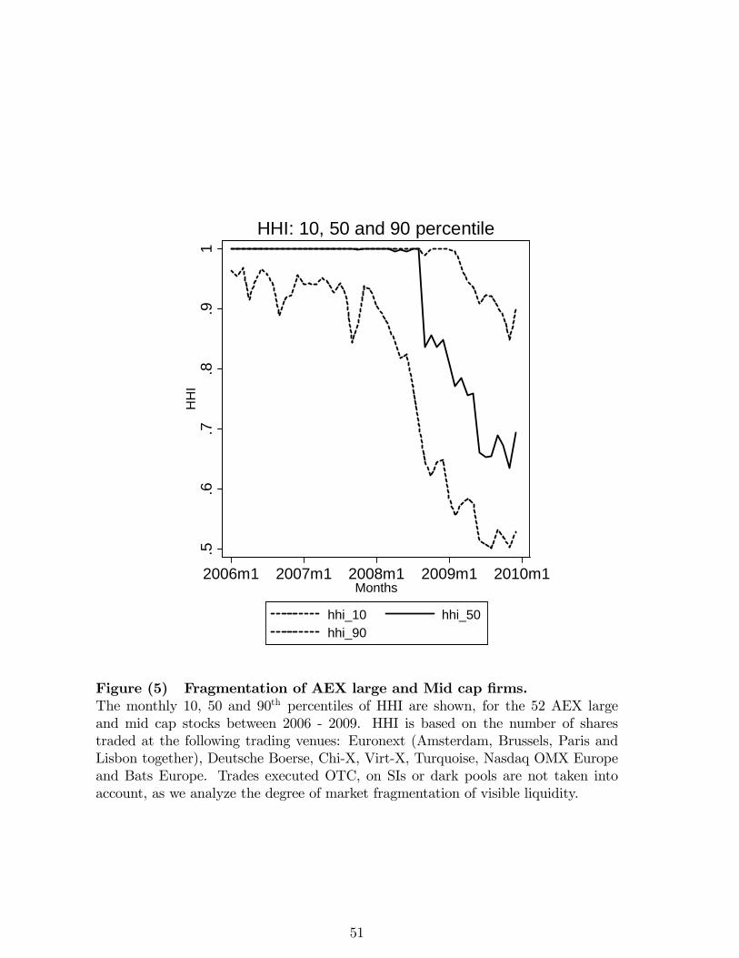
.5.6

.7.8

.91

HH

I

2006m1 2007m1 2008m1 2009m1 2010m1Months

hhi_10 hhi_50hhi_90

HHI: 10, 50 and 90 percentile

Figure (5) Fragmentation of AEX large and Mid cap �rms.The monthly 10, 50 and 90th percentiles of HHI are shown, for the 52 AEX largeand mid cap stocks between 2006 - 2009. HHI is based on the number of sharestraded at the following trading venues: Euronext (Amsterdam, Brussels, Paris andLisbon together), Deutsche Boerse, Chi-X, Virt-X, Turquoise, Nasdaq OMX Europeand Bats Europe. Trades executed OTC, on SIs or dark pools are not taken intoaccount, as we analyze the degree of market fragmentation of visible liquidity.

51

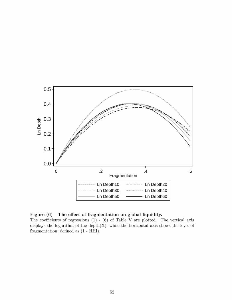
0.0

0.1

0.2

0.3

0.4

0.5

Ln D

epth

0 .2 .4 .6Fragmentation

Ln Depth10 Ln Depth20Ln Depth30 Ln Depth40Ln Depth50 Ln Depth60

Figure (6) The e¤ect of fragmentation on global liquidity.The coe¢ cients of regressions (1) - (6) of Table V are plotted. The vertical axisdisplays the logarithm of the depth(X), while the horizontal axis shows the level offragmentation, de�ned as (1 - HHI).

52

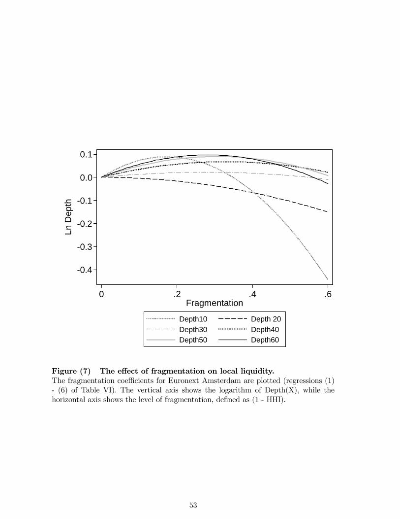
­0.4

­0.3

­0.2

­0.1

0.0

0.1

Ln D

epth

0 .2 .4 .6Fragmentation

Depth10 Depth 20Depth30 Depth40Depth50 Depth60

Figure (7) The e¤ect of fragmentation on local liquidity.The fragmentation coe¢ cients for Euronext Amsterdam are plotted (regressions (1)- (6) of Table VI). The vertical axis shows the logarithm of Depth(X), while thehorizontal axis shows the level of fragmentation, de�ned as (1 - HHI).

53

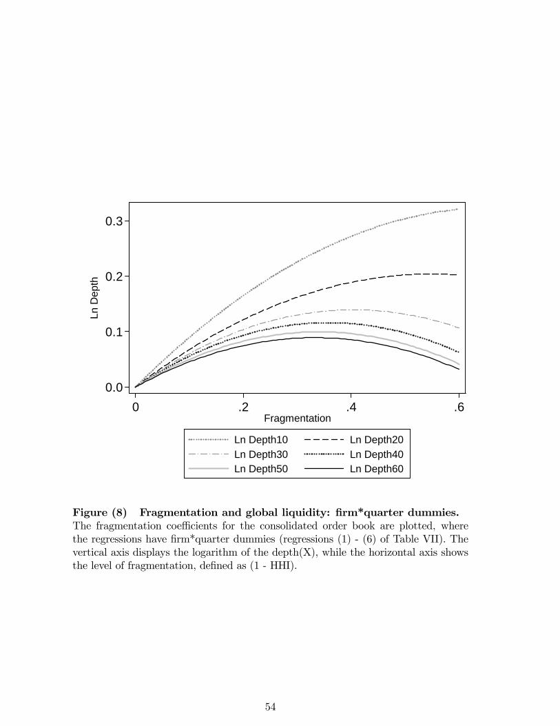
0.0

0.1

0.2

0.3

Ln D

epth

0 .2 .4 .6Fragmentation

Ln Depth10 Ln Depth20Ln Depth30 Ln Depth40Ln Depth50 Ln Depth60

Figure (8) Fragmentation and global liquidity: �rm*quarter dummies.The fragmentation coe¢ cients for the consolidated order book are plotted, wherethe regressions have �rm*quarter dummies (regressions (1) - (6) of Table VII). Thevertical axis displays the logarithm of the depth(X), while the horizontal axis showsthe level of fragmentation, de�ned as (1 - HHI).

54

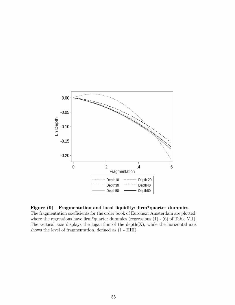
­0.20

­0.15

­0.10

­0.05

0.00

Ln D

epth

0 .2 .4 .6Fragmentation

Depth10 Depth 20Depth30 Depth40Depth50 Depth60

Figure (9) Fragmentation and local liquidity: �rm*quarter dummies.The fragmentation coe¢ cients for the order book of Euronext Amsterdam are plotted,where the regressions have �rm*quarter dummies (regressions (1) - (6) of Table VII).The vertical axis displays the logarithm of the depth(X), while the horizontal axisshows the level of fragmentation, de�ned as (1 - HHI).

55

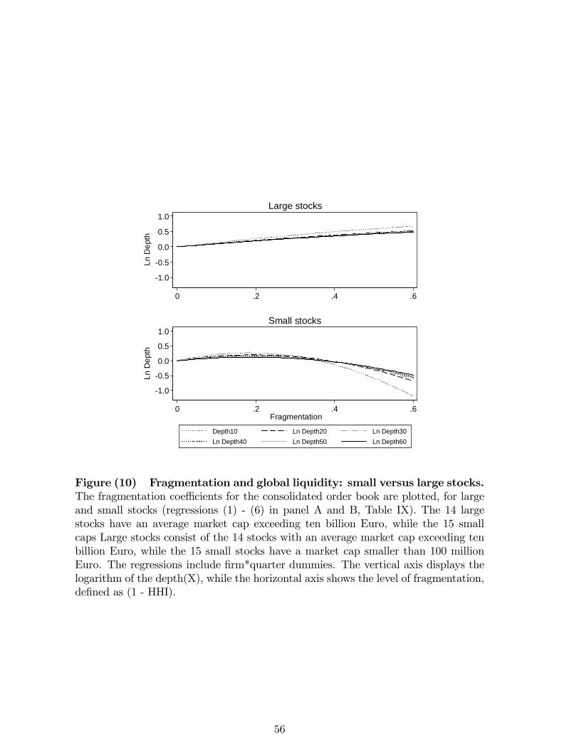
­1.0

­0.5

0.0

0.5

1.0

Ln D

epth

0 .2 .4 .6

Large stocks

­1.0

­0.5

0.0

0.5

1.0

Ln D

epth

0 .2 .4 .6Fragmentation

Depth10 Ln Depth20 Ln Depth30Ln Depth40 Ln Depth50 Ln Depth60

Small stocks

Figure (10) Fragmentation and global liquidity: small versus large stocks.The fragmentation coe¢ cients for the consolidated order book are plotted, for largeand small stocks (regressions (1) - (6) in panel A and B, Table IX). The 14 largestocks have an average market cap exceeding ten billion Euro, while the 15 smallcaps Large stocks consist of the 14 stocks with an average market cap exceeding tenbillion Euro, while the 15 small stocks have a market cap smaller than 100 millionEuro. The regressions include �rm*quarter dummies. The vertical axis displays thelogarithm of the depth(X), while the horizontal axis shows the level of fragmentation,de�ned as (1 - HHI).

56