Erosivity, surface runoff, and soil erosion estimationusing GIS-coupled runoff–erosion model in the Mamuabacatchment, Brazil

Richarde Marques da Silva &

Celso Augusto Guimarães Santos &

Valeriano Carneiro de Lima Silva &

Leonardo Pereira e Silva

Received: 4 November 2012 /Accepted: 24 April 2013 /Published online: 8 May 2013# Springer Science+Business Media Dordrecht 2013

Abstract This study evaluates erosivity, surface run-off generation, and soil erosion rates for Mamuaba catch-ment, sub-catchment of GramameRiver basin (Brazil) byusing the ArcView Soil and Water Assessment Tool(AvSWAT)model. Calibration and validation of themod-el was performed on monthly basis, and it could simulatesurface runoff and soil erosion to a good level of accura-cy. Daily rainfall data between 1969 and 1989 from sixrain gauges were used, and the monthly rainfall erosivityof each station was computed for all the studied years. Inorder to evaluate the calibration and validation of themodel, monthly runoff data between January 1978 andApril 1982 from one runoff gauge were used as well. Theestimated soil loss rates were also realistic when com-pared to what can be observed in the field and toresults from previous studies around of catchment.The long-term average soil loss was estimated at9.4 t ha−1 year−1; most of the area of the catchment

(60 %) was predicted to suffer from a low- tomoderate-erosion risk (<6 t ha−1 year−1) and, in20 % of the catchment, the soil erosion was estimatedto exceed >12 t ha−1 year−1. Expectedly, estimated soilloss was significantly correlated with measured rainfalland simulated surface runoff. Based on the estimatedsoil loss rates, the catchment was divided into fourpriority categories (low, moderate, high and very high)for conservation intervention. The study demonstratesthat the AvSWAT model provides a useful tool for soilerosion assessment from catchments and facilitates theplanning for a sustainable land management in north-eastern Brazil.

Keywords Surface runoff . Soil loss . Catchmenttreatment . Mamuaba catchment

Introduction

Water erosion is one of the most significant environmen-tal degradation processes, and is made up of rill andinterrill erosion. Interrill erosion occurs when soil parti-cles are detached by raindrops and transported by shallowoverland flow, whereas rill erosion is the detachment andtransport of soil particles by concentrated flow. Thisdetached soil is then transported and delivered as sedi-ment downstream. In areas where the erosion process isadvanced, a reduction of agricultural productivity can

Environ Monit Assess (2013) 185:8977–8990DOI 10.1007/s10661-013-3228-x

R. M. da SilvaDepartment of Geosciences, Federal University of Paraíba,58051-900 João Pessoa, Paraíba, Brazile-mail: richarde@geociencias.ufpb.br

C. A. G. Santos (*) :V. C. de Lima Silva : L. P. e SilvaDepartment of Civil and Environmental Engineering,Federal University of Paraíba,58051-900 João Pessoa, Paraíba, Brazile-mail: celso@ct.ufpb.br

occur and the transported sediments, nutrients, and agro-chemicals contaminate and fill up water bodies.

Accelerated soil erosion, mainly caused by water, isa widespread problem affecting environmental quality,agricultural productivity, and food security in manycountries of the world (Santos et al. 2011; Silva et al.2012). Obviously, the economic and social impacts ofsoil erosion are more severe in the developing coun-tries, compared to the developed ones, because of thedirect dependence of livelihood of a large majority oftheir populations on agriculture and land resources(Tibebe and Bewket 2011). Geographically, soil ero-sion is more severe in the tropical highland areas andlower in the temperate regions of the world. It is alsoin these geographic regions that many of the develop-ing countries of the world are situated (Bewket &Teferi 2009; Tripathi et al. 2003).

In Brazil, soil erosion contributes significantly tofood insecurity of rural households and constitutes areal threat to sustainability of the existing subsistenceagriculture (Beskow et al. 2009). Throughout thetwentieth century, the agriculture of northeasternBrazil was responsible for rapid occupation of territo-ry, especially because of two major crops that werecharacteristic of the most important agricultural frontiers(cotton and sugarcane). The sugarcane culture was pre-dominant in northeastern Brazil during the second halfof the century. This crop greatly influenced the country’snational and international economic standing, influencedby pedoclimatic and geomorphological conditions(Castro and Queiroz Neto 2009).

Even though soil erosion is a major environmentaland economic problem in the country, there are only fewmeasurements on the extent of soil loss by the differentprocesses or agents of erosion. Measurements and quan-titative data on magnitudes of soil loss by the differentprocesses, including spatial and temporal patterns, facil-itate conservation planning and setting of spatial prior-ities for intervention.

Such data are useful to understand the extent of theproblem, identify and recommend to land users appro-priate conservation measures, and evaluate effectivenessand efficiency of the measures for possible improve-ment; hence, they are useful to decision makers at var-ious levels. Despite its importance, there is a generaldearth of quantitative information on soil erosion inBrazil (Castro and Queiroz Neto 2009). According toBeskow et al. (2009), quantitative results related to thesoil loss rates and conservation strategies are not usually

available for areas with erosion problems. However,quantitative erosion assessments and possible strategiesfor management of basins are necessary for both localplanning and the governmental agencies associated withsustainable development. Thus, erosion simulationmodels, especially distributed models, are useful toevaluate different strategies for land use and soil man-agement improvement in these watersheds.

Several physically based models have been devel-oped for estimating soil erosion in basins, such as Soiland Water Assessment Tool (SWAT) (Arnold et al.1998), WEPP (Flanagan et al. 2007), LISEM (DeRoo and Jetten 1999), GeoWEPP (Renschler 2003),and SWAT (Parajuli et al. 2008; Ullrich and Volk2009). The SWAT is a physically based, continuoustime-scale model and was developed to simulate theimpact of management on water, sediment, and agri-cultural chemical yields at a basin scale, and its maincomponents are weather, hydrology, soil temperatureand other properties, plant growth, nutrients, pesti-cides, and land management (Gassman et al. 2007).

ArcView Soil and Water Assessment Tool (AvSWAT)is a dynamic and distributed environmental modelingsystem (Green and Van Griensven 2008) based on geo-graphic information systems (GIS), which provides anexcellent environment for modeling. Thus, the aim ofthis study is to identify critical sub-catchments and toevaluate the applicability of SWAT model forMamuaba catchment based on GIS-coupled runoff–erosion model.

The study area

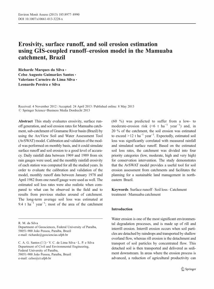
The Mamuaba catchment is located between276 ,678mE/9 ,187 ,399mN and 264 ,489mE/9,196,394mN. It is situated 25 km East from JoãoPessoa, capital of Paraíba State, and forms part of theupstream reach of the Gramame River basin (Fig. 1). Thecatchment has an area of 60.9 km2, and its stream is amajor tributary to the Gramame River. Elevations in thecatchment range from 45 to 215 m above mean sea level.Most of the lower catchment is characterized by gentleslopes, whereas the upper and the middle areas are char-acterized by steep to moderately steep slopes. It is ingeneral, a sub-humid climate in the basin, with a meanannual total rainfall of around 1,700 mm/year, a meanevaporation rate of around 1,300 mm/year (Beltrão et al.2009), and a mean temperature ranging from 23 to 29 °C.

8978 Environ Monit Assess (2013) 185:8977–8990

The catchment has diverse soil types and the majorones are spodic, red Acrisol, yellow Acrisol, and red–yellow Acrisol. The first three (spodic, red Acrisol, andyellow Acrisol) cover more than 43% of the total area ofthe catchment. In terms of land use, six major land useand land cover types can be identified within the catch-ment: pineapple, grassland, livestock, sugarcane cultiva-tion, bare soil, and rainforest. The livestock reared aremainly cattle and sheep in the catchment. Livestock,specifically oxen, provide the means for the farmingoperation and transportation services (bovines), whilecrop residues constitute important sources of livestockfeed. Free grazing is common after crops are harvested.There are also two urban settlements around the catch-ment, namely Pedras de Fogo and Alhandra.

Material and methods

The AvSWAT model

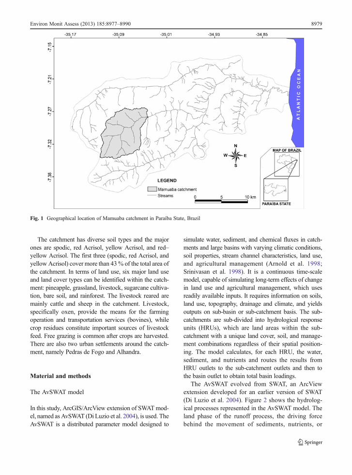
In this study, ArcGIS/ArcView extension of SWATmod-el, named as AvSWAT (Di Luzio et al. 2004), is used. TheAvSWAT is a distributed parameter model designed to

simulate water, sediment, and chemical fluxes in catch-ments and large basins with varying climatic conditions,soil properties, stream channel characteristics, land use,and agricultural management (Arnold et al. 1998;Srinivasan et al. 1998). It is a continuous time-scalemodel, capable of simulating long-term effects of changein land use and agricultural management, which usesreadily available inputs. It requires information on soils,land use, topography, drainage and climate, and yieldsoutputs on sub-basin or sub-catchment basis. The sub-catchments are sub-divided into hydrological responseunits (HRUs), which are land areas within the sub-catchment with a unique land cover, soil, and manage-ment combinations regardless of their spatial position-ing. The model calculates, for each HRU, the water,sediment, and nutrients and routes the results fromHRU outlets to the sub-catchment outlets and then tothe basin outlet to obtain total basin loadings.

The AvSWAT evolved from SWAT, an ArcViewextension developed for an earlier version of SWAT(Di Luzio et al. 2004). Figure 2 shows the hydrolog-ical processes represented in the AvSWAT model. Theland phase of the runoff process, the driving forcebehind the movement of sediments, nutrients, or

Fig. 1 Geographical location of Mamuaba catchment in Paraíba State, Brazil

Environ Monit Assess (2013) 185:8977–8990 8979

pesticides, is simulated by the model based on thefollowing water balance equation:

SW t ¼ SW 0 þXt

i¼1

Ri � Qi � ETi � Pi � Qgi

� �ð1Þ

where, SWt is the final soil water content (in millime-ters), SW0 is the initial soil water content on day i (inmillimeters), t is the time (in days), Ri is the amount ofprecipitation on day i (in millimeters), Qi is the amountof daily surface runoff (in millimeters), ETi is theamount of evapotranspiration on day i (in millimeters),Pi is the amount of water entering the vadose zone fromthe soil profile on day i (in millimeters), and Qgi is theamount of return flow on day i (in millimeters).

Two alternative approaches are provided in the modelfor estimating surface runoff. These are the SoilConservation Service (SCS) curve number (CN) method(USDA-SCS United States Department of Agriculture–Soil Conservation Service 1972) and the Green-Amptinfiltration method. The SCS CN method was used inthis study. The amount of daily surface runoff is given as:

Q ¼ R� Iað Þ2R� Ia þ Sð Þ ð2Þ

where Ia is the initial abstractions which includes surfacestorage, interception, and infiltration prior to runoff (inmillimeters) and S is the retention parameter (in millime-ters). Runoff will only occur when the rainfall depth isgreater than the initial abstractions (i.e., R>Ia). The re-tention parameter varies spatially due to changes in soils,land use, management, and slope and temporally due to

changes in soil water content. The retention parameter isdefined as:

S ¼ 25:41000

CN� 10

� �ð3Þ

where CN is the applicable curve number for the day. Theinitial abstractions, Ia, is commonly approximated as0.2S. Hence, Eq. (2) can be given as:

Q ¼ R� 0:2Sð Þ2R� 0:8Sð Þ ð4Þ

The peak runoff rate, which is the maximum runoffrate that occurs with a given rainfall event, is anindicator of the erosive power of a storm. It is usedto calculate the sediment loss from the unit. SWATcalculates peak runoff rate with a modified rationalmethod which is given as:

qpeak ¼ C � I � A3:6

ð5Þ

where qpeak is the peak runoff rate (in cubic meters persecond), C is the runoff coefficient, I is the rainfallintensity (in millimeters per hour), A is the sub-catchment area (in square kilometers), and 3.6 is a unitconversion factor from millimeters per hour per squarekilometers to cubic meters per second.

The soil evaporation compensation factor (ESCO)is used to adjust the depth distribution for evaporationfrom the soil to account for the effect of capillaryaction, crusting, and cracks. ESCO must be between0.01 and 1.0. As the value for ESCO is reduced, themodel

Fig. 2 Schematic frame-work of the AvSWAT (DiLuzio et al. 2004)

8980 Environ Monit Assess (2013) 185:8977–8990

is able to extract more of the evaporative demand fromlower levels. This coefficient is a calibration parameterand not a property that can be directly measured(Feyereisen et al. 2007). Calibration of these parametersis considered most critical since they may vary from onewatershed to another even within the same geographicalarea.

The AvSWATmodel employs the Modified UniversalSoil Loss Equation (MUSLE) developed by Williamsand Berndt (1977) to compute sediment yield for eachsub-basin.MUSLE is amodified version of the UniversalSoil Loss Equation (USLE) developed by Wischmeierand Smith (1965, 1978). The MUSLE is given as:

Psed ¼ 11:8ðQ � qpeak � AhruÞ0:56 � KUSLE � CUSLE � PUSLE � LSUSLEð6Þ

where, Psed is the sediment yield on a given day (in tons),Q is the surface runoff volume (inmillimeters per hectare),qpeak is the peak runoff rate (in cubic meters per second),Ahru is the area of the HRU (in hectare), KUSLE is theUSLE soil erodibility factor,CUSLE is theUSLE cover andmanagement factor, PUSLE is the USLE support practicefactor, and LSUSLE is the USLE topographic factor.

The AvSWAT model allows for simultaneous com-putations in each sub-catchment and routes the water,sediment, and nutrients from the sub-basin outlets tothe basin outlet. The routing model consists of twocomponents—deposition and degradation, which op-erate simultaneously. The amount of sediment finallyreaching the basin’s outlet, SOUT, is given as:

SOUT ¼ SIN � SD þ DT ð7Þwhere, SIN is the sediment entering the last or final reach,SD is the sediment deposited and DT is total degradation.The total degradation is the sum of re-entrainment andbed degradation components, and it is given as:

DT ¼ Dr þ DBð Þ 1� DRð Þ ð8Þ

where, Dr is the sediment re-entrained, DB is the bedmaterial degradation component, and DR is the sedimentdelivery ratio. Detailed theoretical documentation for themodel is given by Neitsch et al. (2007).

The spatial databases required for the AvSWAT inter-face include topography and drainage network, climate,land use, and soil layers. A brief description of each ofthem is given below.

Topography and drainage network

Topographic and drainage network data were prepared bydigitizing topographic maps of the catchment that wereobtained from the images of Shuttle Radar TopographyMission, available in http://www.glcf.umd.edu/data/srtm.The digitized contour vectors were used to create trian-gular irregular network for generating the DigitalElevation Model (DEM) in 30-m resolution. The DEMand the digitized drainage network were used to delineatethe catchment and its sub-catchments and to analyze thedrainage patterns of the land surface.

Since AvSWAT works on a sub-catchment basis,the catchment was sub-divided into 31 sub-catchmentsand parameters such as surface slope, slope length,and the stream network characteristics such as channelslope, length, and width were derived from the DEM.

Land use and soil types

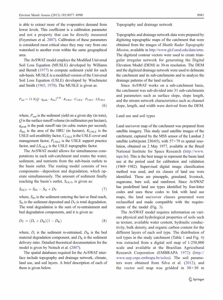
Land use/cover map of the catchment was prepared fromsatellite imagery. This study used satellite images of thecatchment, captured by the MSS sensor of the Landsat 2satellite (orbit/point 230/65), with 57×79 m spatial reso-lution, obtained on 2 May 1977, available at the BrazilNational Institute for Space Research (http://www.inpe.br). This is the best image to represent the basin landuse at the period used for calibration and validation(1969−1982). Supervised digital image classificationmethod was used, and six classes of land use wereidentified. These are pineapple, grassland, livestock,sugarcane, bare soil, and rainforest. Since AvSWAThas predefined land use types identified by four-lettercodes and uses these codes to link with land usemaps, the land use/cover classes generated werereclassified and made compatible with the require-ments of the model (Fig. 3).

The AvSWAT model requires information on vari-ous physical and hydrological properties of soils suchas texture, available water content, hydraulic conduc-tivity, bulk density, and organic carbon content for thedifferent layers of each soil type. The distribution ofsoil types in the study catchment (Table 1 and Fig. 4)was extracted from a digital soil map of 1:250,000scale and available at the Brazilian AgriculturalResearch Corporation (EMBRAPA 1972) (http://www.uep.cnps.embrapa.br/solos). The soil parame-ters were obtained from Silva et al. (2012), andthe vector soil map was gridded in 30×30 m

Environ Monit Assess (2013) 185:8977–8990 8981

resolution, matching the DEM available at theBrazil National Institute for Space Research (http://www.dsr.inpe.br/topodata).

Climate data

AvSWAT requires daily climatic data that can eitherbe read from a measured dataset or generated by aweather generator algorithm. The required climaticvariables include rainfall, minimum and maximumtemperatures, wind speed, solar radiation, and dewpoint temperature. For this study, the available dataat one weather station (Guaraíra station, located atthe coordinates: 273,500mE and 9,193,520 mN)located near by the catchment were used for theperiod 2006–2010 (Table 2). Daily solar radiation,wind speed, relative humidity, and temperaturedata were available from the Guaraíra station,while the daily rainfall data were available fromsix gauges (Table 2).

Computation of rainfall erosivity

Daily rainfall data between 1969 and 1989 from sixrain gauges were used, and the monthly rainfallerosivity of each station was computed. The erosiv-ity was employed to create a database of erosiveevents. The rainfall erosivity factor was calculatedbased on the methodology of Da Silva (2004) as:

R ¼X12

m¼1

89:823Pm

2

Pa

� �0:759

ð9Þ

Fig. 3 Land use/cover map and streams of the Mamuabacatchment

Table 1 Description of main soil types in Mamuaba catchment

Soil types Codes in AvSWAT Percent of total area

Spodic TX047 34.30

Red Acrisol TX236 7.19

Yellow Acrisol TX237 1.35

Red-Yellow Acrisol TX238 57.16

Fig. 4 Soil types, rain gauges and weather gauge in the Mamuabacatchment

Table 2 Location and data range for the rainfall and meteoro-logical gauges

Identification Type Latitude (m) Longitude (m) Altitude

Guaraíra Weather 9,193,520 273,500 125

Santa Emilia Rain 9,183,317 266,355 139

Imbiribeira Rain 9,196,257 273,659 101

Jangada Rain 9,188,865 270,011 125

Salto River Rain 9,190,734 275,524 110

Acau Rain 9,192,520 262,630 146

MamoabaFarm

Rain 9,194,388 268,144 136

8982 Environ Monit Assess (2013) 185:8977–8990

where R is rainfall erosivity factor (in megajoule millime-ter per hectare per hour per year), Pm is monthly rainfall(in millimeters), and Pa is annual mean rainfall (inmillimeters).

Model calibration and validation

Daily discharge data of the Mamuaba River, at theoutlet of the catchment, for the period 1969–1982were used for model calibration and validation.Model calibration was undertaken manually byadjusting sensitive parameters using eight years ofobserved data from January 1969 to December1977. The manual calibration method outlined inthe SWAT Version 2005 user’s manual (Neitsch etal. 2007) was used to minimize the sum of squareddifferences between observed and simulated runoffvalues and maximize correlation coefficient. Validationwas applied after manual calibration of the mostsensitive parameters.

The period of validation was done with five yearsof observed data from January 1978 to April 1982.The most sensitive parameters were found to be theCN and the ESCO. Raising the ESCO value decreasesthe soil depth to which SWAT can satisfy potential soilevaporative demand, thus decreasing soil evaporationand evapotranspiration and increasing total wateryield, stormflow, and baseflow (Santhi et al. 2001;Van Liew and Garbrecht 2003). The model perfor-mance was evaluated through the coefficient ofdetermination (R2) and Nash–Sutcliffe efficiencycoefficient (E) and graphical methods of compar-ing simulated and observed data.

Results and Discussion

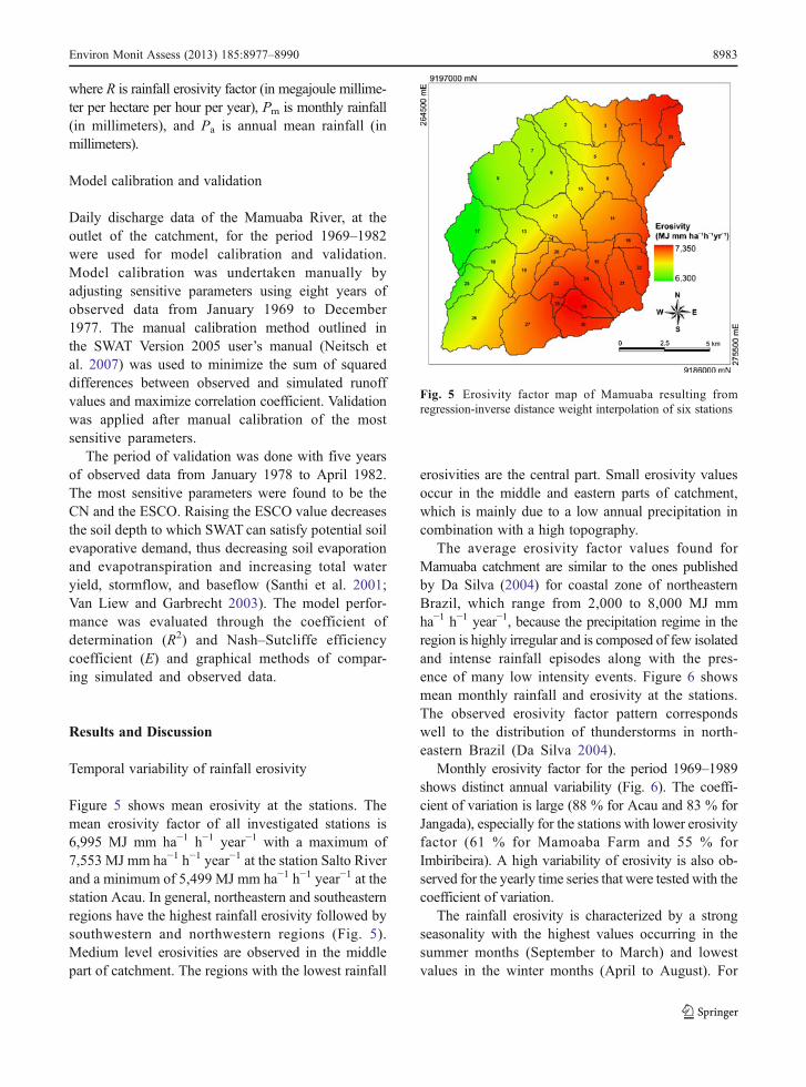
Temporal variability of rainfall erosivity

Figure 5 shows mean erosivity at the stations. Themean erosivity factor of all investigated stations is6,995 MJ mm ha−1 h−1 year−1 with a maximum of7,553 MJ mm ha−1 h−1 year−1 at the station Salto Riverand a minimum of 5,499 MJ mm ha−1 h−1 year−1 at thestation Acau. In general, northeastern and southeasternregions have the highest rainfall erosivity followed bysouthwestern and northwestern regions (Fig. 5).Medium level erosivities are observed in the middlepart of catchment. The regions with the lowest rainfall

erosivities are the central part. Small erosivity valuesoccur in the middle and eastern parts of catchment,which is mainly due to a low annual precipitation incombination with a high topography.

The average erosivity factor values found forMamuaba catchment are similar to the ones publishedby Da Silva (2004) for coastal zone of northeasternBrazil, which range from 2,000 to 8,000 MJ mmha−1 h−1 year−1, because the precipitation regime in theregion is highly irregular and is composed of few isolatedand intense rainfall episodes along with the pres-ence of many low intensity events. Figure 6 showsmean monthly rainfall and erosivity at the stations.The observed erosivity factor pattern correspondswell to the distribution of thunderstorms in north-eastern Brazil (Da Silva 2004).

Monthly erosivity factor for the period 1969–1989shows distinct annual variability (Fig. 6). The coeffi-cient of variation is large (88 % for Acau and 83 % forJangada), especially for the stations with lower erosivityfactor (61 % for Mamoaba Farm and 55 % forImbiribeira). A high variability of erosivity is also ob-served for the yearly time series that were tested with thecoefficient of variation.

The rainfall erosivity is characterized by a strongseasonality with the highest values occurring in thesummer months (September to March) and lowestvalues in the winter months (April to August). For

Fig. 5 Erosivity factor map of Mamuaba resulting fromregression-inverse distance weight interpolation of six stations

Environ Monit Assess (2013) 185:8977–8990 8983

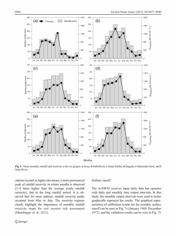
stations located at higher elevations, a more pronouncedpeak of rainfall erosivity in winter months is observed(3–4 times higher than the average yearly rainfallerosivity), due to the long rainfall period. It is ob-served that for most stations, rainfall erosivity peaksoccurred from May to July. The erosivity regimesclearly highlight the importance of monthly rainfallerosivity maps for soil erosion risk assessment(Meusburger et al. 2012).

Surface runoff

The AvSWAT receives input daily data but operateswith daily and monthly time output intervals. In thisstudy, the monthly output intervals were used to bettergraphically represent the results. The graphical repre-sentation of calibration results for the monthly surfacerunoff can be seen in Fig. 7a (January 1969–December1977), and the validation results can be seen in Fig. 7b

Jan Feb Mar Apr May Jun Jul Aug Sep Oct Nov Dec0

50

100

150

200

250

300

Mon

thly

rain

fall

(mm

)

0

400

800

1200

1600

2000

Jan Feb Mar Apr May Jun Jul Aug Sep Oct Nov Dec0

50

100

150

200

250

300

0

400

800

1200

1600

2000

EI m

onth

ly(M

Jm

mha

- ¹h-

¹)

(b)

Jan Feb Mar Apr May Jun Jul Aug Sep Oct Nov Dec

Mon

thly

rain

fall

(mm

)

0

400

800

1200

1600

2000

Jan Feb Mar Apr May Jun Jul Aug Sep Oct Nov Dec0

50

100

150

200

250

300

0

400

800

1200

1600

2000

EIm

onth

ly(M

Jm

mh

a-¹h

- ¹)

(d)

Jan Feb Mar Apr May Jun Jul Aug Sep Oct Nov Dec0

50

100

150

200

250

300

Mon

thly

rain

fall

(mm

)

0

400

800

1200

1600

2000

Jan Feb Mar Apr May Jun Jul Aug Sep Oct Nov Dec0

50

100

150

200

250

300

0

400

800

1200

1600

2000

EI m

onth

ly(M

Jm

mha

- ¹h-

¹)

(f)

Months

EImonthly Rainfall (mm)(a)

(c)

(e)

Fig. 6 Mean monthly rainfall and erosivity at the six gauges: a Acau, b Imbiribeira, c Santa Emilia, d Jangada, eMamoaba Farm, and fSalto River

8984 Environ Monit Assess (2013) 185:8977–8990

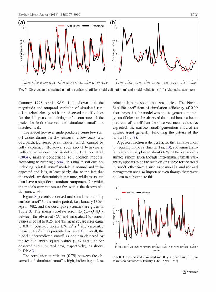
(January 1978–April 1982). It is shown that themagnitude and temporal variation of simulated run-off matched closely with the observed runoff valuesfor the 14 years and timings of occurrence of thepeaks for both observed and simulated runoff notmatched well.

The model however underpredicted some low run-off values during the dry season in a few years, andoverpredicted some peak values, which cannot befully explained. However, such model behavior iswell-known as described in detail by Di Luzio et al.(2004), mainly concerning soil erosion models.According to Nearing (1998), this bias in soil erosion,including rainfall–runoff models is normal and to beexpected and it is, at least partly, due to the fact thatthe models are deterministic in nature, while measureddata have a significant random component for whichthe models cannot account for, within the determinis-tic framework.

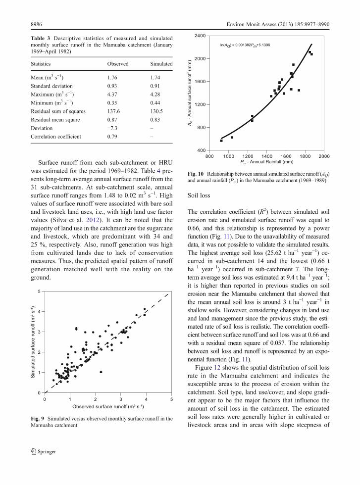
Figure 8 presents observed and simulated monthlysurface runoff for the entire period, i.e., January 1969–April 1982, and the descriptive statistics are given inTable 3. The mean absolute error, Σ(|Qo−Qs|/Qo),between the observed (Qo) and simulated (Qs) runoffvalues is equal to 0.25, and the mean square error equalto 0.017 (observed mean 1.76 m3 s−1 and calculatedmean 1.74 m3 s−1 as presented in Table 3). Overall, themodel underpredicted runoff, as one can observed bythe residual mean square values (0.87 and 0.83 forobserved and simulated data, respectively), as shownin Table 3.

The correlation coefficient (0.79) between the ob-served and simulated runoff is high, indicating a close

relationship between the two series. The Nash–Sutcliffe coefficient of simulation efficiency of 0.99also shows that the model was able to generate month-ly runoff close to the observed data, and hence a betterpredictor of runoff than the observed mean value. Asexpected, the surface runoff generation showed anupward trend generally following the pattern of therainfall (Fig. 9).

A power function is the best fit for the rainfall–runoffrelationship in the catchment (Fig. 10), and annual rain-fall variability explained about 66 % of the variance insurface runoff. Even though inter-annual rainfall vari-ability appears to be the main driving force for the trendin runoff, other factors such as changes in land use andmanagement are also important even though there wereno data to substantiate this.

Fig. 7 Observed and simulated monthly surface runoff for model calibration (a) and model validation (b) for Mamuaba catchment

Fig. 8 Observed and simulated monthly surface runoff in theMamuaba catchment (January 1969–April 1982)

Environ Monit Assess (2013) 185:8977–8990 8985

Surface runoff from each sub-catchment or HRUwas estimated for the period 1969–1982. Table 4 pre-sents long-term average annual surface runoff from the31 sub-catchments. At sub-catchment scale, annualsurface runoff ranges from 1.48 to 0.02 m3 s−1. Highvalues of surface runoff were associated with bare soiland livestock land uses, i.e., with high land use factorvalues (Silva et al. 2012). It can be noted that themajority of land use in the catchment are the sugarcaneand livestock, which are predominant with 34 and25 %, respectively. Also, runoff generation was highfrom cultivated lands due to lack of conservationmeasures. Thus, the predicted spatial pattern of runoffgeneration matched well with the reality on theground.

Soil loss

The correlation coefficient (R2) between simulated soilerosion rate and simulated surface runoff was equal to0.66, and this relationship is represented by a powerfunction (Fig. 11). Due to the unavailability of measureddata, it was not possible to validate the simulated results.The highest average soil loss (25.62 t ha−1 year−1) oc-curred in sub-catchment 14 and the lowest (0.66 tha−1 year−1) occurred in sub-catchment 7. The long-term average soil loss was estimated at 9.4 t ha−1 year−1;it is higher than reported in previous studies on soilerosion near the Mamuaba catchment that showed thatthe mean annual soil loss is around 3 t ha−1 year−1 inshallow soils. However, considering changes in land useand land management since the previous study, the esti-mated rate of soil loss is realistic. The correlation coeffi-cient between surface runoff and soil loss was at 0.66 andwith a residual mean square of 0.057. The relationshipbetween soil loss and runoff is represented by an expo-nential function (Fig. 11).

Figure 12 shows the spatial distribution of soil lossrate in the Mamuaba catchment and indicates thesusceptible areas to the process of erosion within thecatchment. Soil type, land use/cover, and slope gradi-ent appear to be the major factors that influence theamount of soil loss in the catchment. The estimatedsoil loss rates were generally higher in cultivated orlivestock areas and in areas with slope steepness of

Table 3 Descriptive statistics of measured and simulatedmonthly surface runoff in the Mamuaba catchment (January1969–April 1982)

Statistics Observed Simulated

Mean (m3 s−1) 1.76 1.74

Standard deviation 0.93 0.91

Maximum (m3 s−1) 4.37 4.28

Minimum (m3 s−1) 0.35 0.44

Residual sum of squares 137.6 130.5

Residual mean square 0.87 0.83

Deviation −7.3 –

Correlation coefficient 0.79 –

Fig. 9 Simulated versus observed monthly surface runoff in theMamuaba catchment

Fig. 10 Relationship between annual simulated surface runoff (AQ)and annual rainfall (Pm) in the Mamuaba catchment (1969–1989)

8986 Environ Monit Assess (2013) 185:8977–8990

over 30 %. These are also the areas where runoffgeneration was the highest in the catchment. Thenature of the soils and high sandy content, combinedwith the steep slopes and cultivation practices thatlacked conservation measures, contributed to bothhigh-surface runoff and soil loss. The estimatedsoil loss rates were generally lower in the areasunder rainforest cover and grassland with yellowAcrisol soil types. Thus, it can be confirmed that

the land cover plays an important role in the soilerosion process because estimated soil loss rateswere low in areas covered with rainforests regard-less of slope gradients.

Sub-catchment prioritization for treatment

Based on the drainage system, the Mamuaba catchmentwas divided into 31 sub-catchments and the erosionhazard map (Fig. 12) was reclassified for the prioritiza-tion. Based on the estimated annual soil loss rates, the

Table 4 Average annual surface runoff and soil loss from sub-catchments/HRUs

Sub-catchment/HRU

Area(ha)

Averagerainfall(mm)

Averagesurface runoff(m3 s−1)

Soil loss(t ha−1)

1 228.3 1.395 0.058 1.95

2 242.6 1.364 0.052 10.17

3 186.0 1.364 0.042 1.34

4 333.7 1.395 1.385 8.90

5 170.9 1.364 0.132 1.84

6 168.2 1.364 1.171 13.54

7 158.4 1.364 0.034 0.66

8 417.2 1.364 0.093 1.12

9 276.2 1.364 0.187 1.15

10 167.2 1.364 0.919 10.65

11 310.5 1.441 0.210 1.50

12 276.6 1.364 0.695 5.22

13 168.3 1.364 0.337 3.31

14 12.4 1.441 0.301 25.62

15 123.0 1.441 0.029 26.54

16 58.9 1.441 0.099 4.07

17 333.2 1.364 0.080 1.05

18 213.0 1.441 0.216 2.09

19 152.6 1.441 0.042 2.20

20 80.4 1.441 0.256 6.45

21 195.6 1.441 0.052 23.27

22 112.8 1.441 0.031 22.30

23 134.6 1.441 0.188 2.95

24 209.7 1.441 0.048 26.34

25 112.6 1.441 0.032 1.54

26 469.6 1.441 0.126 3.79

27 367.8 1.441 0.095 6.97

28 22.5 1.441 0.062 4.16

29 108.8 1.441 0.024 32.19

30 139.7 1.441 0.032 17.18

31 136.4 1.395 1.478 22.51

0 0.1 0.2 0.3 0.4 0.50.05 0.15 0.25 0.35 0.45

AQ - Annual surface runoff (m³ s-¹)

0.0

0.2

0.4

0.6

0.8

1.0

Sy

-S

oill

oss

( tha

- ¹)

ln(Sy) = 4.1065AQ - 1.7874

Fig. 11 Relationship between simulated soil erosion rate (Sy)and simulated surface runoff (AQ)

Fig. 12 Estimated soil erosion rates (in tons per hectare peryear) in the Mamuaba catchment

Environ Monit Assess (2013) 185:8977–8990 8987

areas were classified in four erosion severity classes. Itwas observed that 14 out of 31 sub-catchments fellunder high or very high soil erosion categories(>6 t ha−1 year−1), of which 5 catchments (2, 4, 10, 20,and 27) were in the high category and 9 catchments (14,15, 21, 22, 24, 27, 29, 30, and 31) were in the very highcategory (Fig. 13).

These two groups of sub-catchments cover slightlyover 38 % of the total area of the catchment (Table 5).Accordingly, most of the area of the catchment (62 %)was considered to suffer from a low- or moderate-erosion risk, which is <6 t ha−1 year−1. Estimated soilloss rates are <3 t ha−1 year−1 in about 44 % of thecatchment. In about 20 % of the catchment, the soilerosion was estimated to exceed 12 t ha−1 year−1. Thisis found in the middle and lower parts of the catchmentwhere steeplands are cultivated and are overgrazed,respectively. Soil erosion is moderate or low largely inthe upper part of the basin with natural vegetation cover,which rarely exceeded 3 t ha−1 year−1.

Conclusions

The aim of this study was to assess erosivity, surfacerunoff generation, and soil erosion rates for theMamuaba catchment in the Gramame River basin ofBrazil by applying the AvSWAT model. The resultsobtained by the present study demonstrated the impor-tance of land cover for the catchment management. TheMamuaba catchment have soils with high vulnerabilityto erosion, high slope steepness, and high rainfall ero-sivity factor, which ranges from 5,550 to 7,550 MJmm ha−1 h−1 year−1.

The simulated surface runoff closely matched withthe observed runoff, and the mean difference wasstatistically nonsignificant. Surface runoff generationvaried among the sub-catchments, and it was generallyhigher in sub-catchments characterized by sugarcaneand livestock land uses and slope gradients greaterthan 25 %.

The estimated soil loss rates were generally higher incultivated areas with slope gradients greater than 35 %.These are also the areas where runoff generation was atits highest value within the catchment. Based on thepredicted annual soil loss values, the catchment wasdivided into four priority categories for conservationintervention. Nine sub-catchments, out of the 31 in thecatchment, were assigned as first priority, 5 fell in thesecond, 4 in the third, and 12 in the fourth priorities.

The prioritization of sub-catchments for conservationis important given the resource constraints to simulta-neously treat the entire catchment. Finally, the studydemonstrates that the AvSWAT model provides a usefultool to predict surface runoff generation patterns and soilerosion hazard over catchments and facilitates planningfor a sustainable land management. Even though theestimated soil erosion rates may not be precise, the re-sults are quite useful since that measured data areunavailable. On the other hand, obtaining the sameinformation by field surveys would take a long timeand considerable human resources. The method can thus

Fig. 13 Categorization of sub-catchments for treatment in theMamuaba catchment

Table 5 Annual soil erosionrates and severity classes in theMamuaba catchment

Soil loss(t ha−1 year−1)

Severity classes Area (ha) Percent oftotal area

Percent of totalsoil loss

Conservationpriority

0–3 Low 26,936 44.2 6.1 Fourth

3–6 Moderate 9,958 16.4 6.4 Third

6–12 High 11,917 19.6 13.5 Second

>12 Very High 12,066 19.8 74.0 First

8988 Environ Monit Assess (2013) 185:8977–8990

be applied in other catchments for assessment and de-lineation of erosion-prone areas for prioritization of sub-catchments for conservation intervention and enableefficient use of the limited resources.

References

Arnold, J. G., Srinivasan, R., Muttiah, R. S., & Williams, J. R.(1998). Large area hydrologic modeling and assessment.Part I: model development. J Amer Water Resour Assoc,34(1), 73–89. doi:10.1111/j.1752-1688.1998.tb05961.x.

Beltrão, G. B. M., Medeiros, E. S. F., & Ramos, R. T. C. (2009).Effects of riparian vegetation on the structure of the marginalaquatic habitat and the associated fish assemblage in a trop-ical Brazilian reservoir. Biota Neotrop, 9(4), 37–43.

Beskow, S., Mello, C. R., Norton, L. D., Curi, N., Viola, M. R.,& Avanzi, J. C. (2009). Soil erosion prediction in theGrande River Basin, Brazil using distributed modelling.Catena, 79(1), 49–59. doi:10.1016/j.catena.2009.05.010.

Bewket, W., & Teferi, E. (2009). Assessment of soil erosion hazardand prioritization for treatment at the catchment level: casestudy in the Chemoga catchment, Blue Nile Basin, Ethiopia.Land Degrad Dev, 20(7), 609–622. doi:10.1002/ldr.944.

Castro, S. S., & Queiroz Neto, J. P. (2009). Soil erosion in Brazilfrom coffee to the present-day soy bean production. DevelopEarth Surf Process, 13(2), 195–221. doi:10.1016/S0928-2025(08)10011-6.

Da Silva, A. M. (2004). Rainfall erosivity map for Brazil. Catena,57(2), 251–259. doi:10.1016/j.catena.2003.11.006.

De Roo, A. P. J., & Jetten, V. G. (1999). Calibrating andvalidating the LISEM model for two data sets from theNetherlands and South Africa. Catena, 37(4), 477–493.doi:10.1016/S0341-8162(99)00034-X.

Di Luzio, M., Srinivasan, R., & Arnold, J. G. (2004). A GIS-coupled hydrological model system for the catchment assess-ment of agricultural nonpoint and point sources of pollution.Transactions in GIS, 8(1), 113–136. doi:10.1111/j.1467-9671.2004.00170.x.

EMBRAPA – Brazilian Agricultural Research Corporation.Levantamento Exploratório: Reconhecimento de solos doEstado da Paraíba na Escala: 1:250.000. Recife, Embrapa,1972.

Feyereisen, G. W., Strickland, T. C., Bosch, D. D., & Sullivan,D. G. (2007). Evaluation of SWAT manual calibration andinput parameter sensitivity in the little river watershed.Transactions of the ASABE, 50(3), 843–855.

Flanagan, D. C., Gilley, J. E., & Franti, T. G. (2007). WaterErosion Prediction Project (WEPP): Development history,model capabilities, and future enhancements. Transactionsof the ASABE, 50(5), 1603–1612.

Gassman, P. W., Reyes, M. R., Green, C. H., & Arnold, J. G.(2007). The soil and water assessment tool: Historicaldevelopment, applications, and future research directions.Transactions of the ASABE, 50(4), 1211–1250.

Green, C. H., & Van Griensven, A. (2008). Autocalibration inhydrologic modeling: using SWAT 2005 in small-scale

watersheds. Environ Model Soft, 23(4), 422–434.doi:10.1016/j.envsoft.2007.06.002.

Meusburger, K., Steel, A., Panagos, P., Montanarella, L., &Alewell, C. (2012). Spatial and temporal variability ofrainfall erosivity factor for Switzerland. Hydrol Earth SystSci, 16(1), 167–177. doi:10.5194/hess-16-167-2012.

Nearing, M. (1998). Why soil erosion models over-predict smallsoil losses and under-predict large soil losses. Catena,32(1), 15–22. doi:10.1016/S0341-8162(97)00052-0.

Neitsch, S. L., Arnold, J. G., Kiniry, J. R., Srinivasan, R.,Williams, J. R. (2007) Soil and water assessment tool input/output file documentation version 2005. Available in: http://twri.tamu.edu/reports/2011/tr406.pdf. Accessed 16December 2011.

Parajuli, P. B., Mankin, K. R., & Barnes, P. L. (2008). Applicabilityof targeting vegetative filter strips to abate fecal bacteria andsediment yield using SWAT. Agric Water Manage, 95(10),1189–1200. doi:10.1016/j.agwat.2008.05.006.

Renschler, C. S. (2003). Designing geo-spatial interfaces to scaleprocess models: The GeoWEPP approach. HydrologicalProcesses, 17(5), 1005–1017. doi:10.1002/hyp.1177.

Santhi, C., Arnold, J. G., Williams, J. R., Dugas, W. A., Srinivasan,R., & Hauck, L. (2001). Validation of the SWAT model on alarge river basin with point and nonpoint sources. Journal ofthe AmericanWater Resources Association, 37(5), 1169–1187.doi:10.1111/j.1752-1688.2001.tb03630.x.

Santos, C., Freire, P., Silva, R.M., Arruda, P., &Mishra, S. (2011).Influence of the catchment discretization on the optimizationof runoff-erosion modelling. J Urban Environ Engng, 5(2),91–102. doi:10.4090/juee.2009.v5n2.091102.

Silva, R. M., Montenegro, S. M. G., & Santos, C. A. G. (2012).Integration of GIS and remote sensing for estimation of soilloss and prioritization of critical sub-catchments: A casestudy of Tapacurá catchment. Nat Hazards, 63(3), 576–592. doi:10.1007/s11069-012-0128-2.

Srinivasan, R., Ramanarayanan, T. S., Arnold, J. G., &Bednarz, S. T. (1998). Large area hydrologic modelingand assessment part II: Model application. J AmericanWater Resour Assoc, 34(1), 91–101. doi:10.1111/j.1752-1688.1998.tb05962.x.

Tibebe, D., & Bewket, W. (2011). Surface runoff and soilerosion estimation using the SWAT model in the Keletacatchment, Ethiopia. Land Degrad Dev, 22(6), 551–564.doi:10.1002/ldr.1034.

Tripathi, M. P., Panda, R. K., & Raghuwanshi, N. S. (2003).Identification and prioritization of critical sub-watershedsfor soil conservation management using the SWAT model.Biosyst Engin, 85(3), 365–379. doi:10.1016/S1537-5110(03)00066-7.

Ullrich, A., & Volk, M. (2009). Application of the Soil andWater Assessment Tool (SWAT) to predict the impact ofalternative management practices on water quality andquantity. Agric Water Manage, 96(10), 1189–1200.doi:10.1016/j.agwat.2009.03.010.

USDA-SCS (United States Department of Agriculture–SoilConservation Service). (1972). National EngineeringHandbook, Section 4 Hydrology. USDA: Washington,DC.

Van Liew, M. W., & Garbrecht, J. (2003). Hydrologic simula-tion of the Little Washita river experimental watershedusing SWAT. Journal of the American Water Resources

Environ Monit Assess (2013) 185:8977–8990 8989

Association, 39(2), 413–426. doi:10.1111/j.1752-1688.2003.tb04395.x.

Williams, J. R., & Berndt, H. D. (1977). Sediment yield predic-tion based on catchment hydrology. Transactions of theASABE, 20(6), 1100–1104.

Wischmeier, W. H., & Smith, D. D. (1965). Predicting rain-fall erosion losses from cropland: a guide for selection of

practices for soil and water conservation (p. 282).USDA Agricultural Handbook. U.S. Department ofAgriculture: Washington, DC.

Wischmeier, W. H., & Smith, D. D. (1978). Predicting rainfallerosion loss: A guide to conservation planning. USDAAgricultural Handbook (p. 537). Washington, DC: U.S.Department of Agriculture.

8990 Environ Monit Assess (2013) 185:8977–8990