SOFT IN SOFT OUT REED SOLOMON DECODING

DEPARTMENT OF COMMUNICATION SYSTEMS

FACULTY OF APPLIED SCIENCES

"In the name of Allah, most Gracious, most Compassionate".

AbstractThe dissertation describes the understanding of Reed Solomon Codes and presents a soft decision decoding algorithm decoder. How performance objectives are established for more reliable digital transmission. Discussing its efficient capability for correcting or removing nearly every type and mixed probability of errors in a signal. Different approaches for building an algorithm for reducing maximum errors in a transmission. Understanding and development of an algorithm for using the efficient capability of RS codes for reducing mixed types of errors in a signal.

So far Hard In Hard Out and Soft In Hard Out approaches are been used. This project deals with the understanding of Soft In Soft Out decoding approach and using reference algorithm “Vardy and Be’ery Decomposition [1]” for developing effective Soft In Soft Out Simulation Decoder based on Reed Solomon Codes and BCH extended matrix.

In this simulation a trellis structure, know as wolf trellis has been implemented in decoding section according to the decomposition factor graph from Vardy & Be’ery research [2]. In this document, simulation results for RS (15, 13, 4) & (7, 5, 4) are presented which are compared by uncoded BPSK (15). All the theoretical material simulation was verified in laboratory.

The Bit Error Rate is calculated exactly for a binary channel and the results are for Gaussian noise. In many wire-line systems, broadband impulse noise is also significant transmission impairment. Although impulse, noise effects are not modelled in this analysis.

The results shows that the method provides significant gain over uncoded BPSK modulator and could compares favourably with the other popular soft decision decoding methods. All the simulation results are written in C language.

TABLE OF CONTENTS PAGE NO

1. Introduction........................................................................................................1

1.1 Modern Era Of Digital Communication........................................................1

1.2 History Of Error Coding.................................................................................2

1.2.1 Types Of Coded.......................................................................................2

1.2.2 Forward Error Correction.........................................................................3

1.2.4 Soft Decision Decoding...........................................................................3

1.3 Types Of Errors................................................................................................4

1.4 A Brief Intro of Reed Solomon Codes............................................................4

1.5 Purpose & Overview of Thesis........................................................................4

2. Reed Solomon Codes......................................................................................5

2.1 Historical Development Of RS Codes............................................................5

2.1.1 Galois Field..............................................................................................6

2.2 Characteristic...................................................................................................6

2.2.1 Parameters................................................................................................6

2.2.2. Code Rate (R) ..........................................................................................7

2.2.3 Correction powers Of RS Codes..............................................................7

2.3 Encoding Approaches......................................................................................8

2.3.1 Original Approach To Reed-Solomon Codes..........................................8

2.3.2. Generator Polynomial Approach .............................................................8

2.3.3 Galois Field Fourier Transform Approach...............................................9

2.4 Decoding Approaches......................................................................................9

2.4.1 Syndrom-Based Decoding.......................................................................9

2.4.2. Algebric Decoding ................................................................................11

2.4.3 Transform Decoding..............................................................................11

2.5 Performance Examples..................................................................................12

2.6 Summary.........................................................................................................13

2.6.1 Coding Gain...........................................................................................13

3. Soft In Soft Out ...............................................................................................14

3.1 Description .....................................................................................................14

3.2 Soft Algorithm Classification .......................................................................14

3.2.1 Reliability Based Decodign..................................................................14

3.2.2 Structure Based Decoding....................................................................14

4. Implementating SISO......................................................................................15

4.1 Implementation Goals....................................................................................15

4.2 Overall Architecture......................................................................................16

4.2.1 RS Interleaving Nature.........................................................................16

4.3 Technique Applied.........................................................................................16

4.3.1 Structure of The Generator Matrix.......................................................16

4.3.2 Encoding..............................................................................................17

4.3.3 RS Factor Graph...................................................................................18

5. Performance Measures..................................................................................20

5.1 AWGN Channel.............................................................................................20

5.2 Simulation Result...........................................................................................20

5.2.1 Complexity...........................................................................................21

6. Further Research.............................................................................................22

7. Conclusion........................................................................................................22

References..............................................................................................................233

Appendix A- .............................................................................................................24

LIST OF FIGURES PAGE NO

Figure 2.1: RS Encoded Structure ......................................................................................... 7

Figure 2.2: Decoder Arhitecture ......................................................................................... 10

Figure 2.3: Referencing Results Using Different RS Algorithms ................................... 12

Figure 4.1: Model of a Reed - Solomon Coded Digital Communication System ......... 15

Figure 4.2: Generator Matrix of Binary Image Of CRS whereB generates CBCH..........16

Figure 4.3: BCH Extended Matrix Structure...............................................................18

Figure 4.4: RS Code Factor Graph based on the Vardy-Be'ery Decomposition.........19

Figure 5.1: Simulation Result; comparision within (15,13,4) & (7,5,4) RS Codes.....20

Figure 5.2: Performance Of Reed-Solomon with Vardy-Be'ery Algorithm Decoding in AWGN Channel..............................................................................................................21

1. IntroductionAs demand for reliable digital communication is increasing, new techniques are evolving, algorithm and codes to reduce the error probability in signals at the receiving end. The project is associated with the ‘Error Correction’ Field. Error coding is used from long time. Different codes are been discovered and invented. When signal is passed through the noise, different types of errors are induced. Every code works with respective to the type of error. So far, Reed Solomon codes are most efficient ones regarding reducing errors. They can work effectively for nearly all types of errors [7]. Different techniques and researches are introduced for using the RS codes capability for removing or correcting error to full extent.

1.1 Modern Era Of Digital Communication

Increasing demand for traditional services has been an important factor in the development of telecommunications technologies. Such developments, combined with more general advances in electronics & computing, have made possible the provision of entirely new communications services.

An important objective in the design of a communications system is often to minimise equipment cost, complexity & power consumption whilst also minimising the bandwidth occupied by the signal and/or transmission time.

Reliable transmission of information is one of the central topics in digital communications. While the advent of powerful digital computing and storage technologies has made the data traffic increasingly digital, the reality of inherently nosy communication channels persists and has thus made error control coding an important and necessary step in achieving reliable communication. Coding in this case refers to systematically introducing redundancy in a message prior to transmission and using thus redundancy to recover the original message the erroneously received one.

Source Coding (Encoding) is concerned with efficient coding, and rate-distortion theory. Source coding is concerned with efficient representation of information generated by a source, and usually attempts to reduce the amount of redundancy in the source information so that as high an information transmission rate can be achieved as is possible without jeopardizing the fidelity of the original source output.[4]

Channel coding (Decoding) is necessary for minimizing the error rate in the received symbols when transmitting information over a noisy channel.

1.2 History Of Error Coding

In the nearly four decades that have passed since the original work of Shannon, Hamming & Golay error control coding has matured into an important branch of communication system engineering. The field of coding has yielded a great many

1

results on the mathematical structure of the codes as well as a number of very efficient coding techniques.

Consequently, steady increase in use of error- control coding in a variety of digital communication systems.

The basic theorems of information theory not only mark the limits of efficiency in communication performance but also define the role that coding plays in achieving these limits. [4]

Shannon’s 1948 paper presented a statistical formulation of the communication problem, unifying earlier work. Shannon’s results showed that as long as the information transmission rate is below capacity, the probability of error in the information delivered can in principle be made arbitrarily low by using sufficiently long coded transmission signals and according to this result, this thesis is based relating to the use of Reed Solomon Codes. Thus, noise limits the achievable information communication rate but not the achievable accuracy. [4]

1.2.1 Types Of Codes

The two main classes of error-correcting codes, which are linear block codes, cyclic codes and convolutional codes. These are briefly described below to get background understanding.

Linear block code is the primary type of channel coding which was used in earlier mobile communication systems. Simply it adds redundancy in order that at the receiver, one can decode with (theoretical) probability of zero errors, provided that the information rate (amount of transported information in bits per sec) would not exceed the channel capacity. The main characterisation of a block code is that it is a fixed length channel code.

Convolutional codes are generally more complicated than linear block codes, more difficult to implement, and have lower code rates (usually below 0.90), but have powerful error correcting capabilities. They are popular in satellite and deep space communications, where bandwidth is essentially unlimited, but the BER is much higher and retransmissions are infeasible.

Convolutional codes are more difficult to decode because they are encoded using finite state machines that have branching paths for encoding each bit in the data sequence.

1.2.2 Forward Error Control

In digital communication, forward error correction (FEC) is a system of error control for data transmission. It differs from standard error detection and correction in that the technique is specifically designed to allow the receiver to correct errors in the currently received data without having to wait for the rest of the message to come in. The important distinction between forward correction, and other detection and correction methods, such as cyclic redundancy check (CRC) or other codes is that in CRC, you need to have all of the bits protected by the checksum received, so that you can compute the CRC of the whole. The difference between forward correction and CRC correction is that in forward correction, it is only the bits already received that are used to correct the "current" bit.

2

1.2.3 Soft-Decision Decoding

Channel noise is almost always a continuous phenomenon. What is transmitted may be selected from a discrete set, but what is received comes from a continuum of values. This leads to the soft-decision decoder (SDD), which accepts a vector of real samples of the noisy channel output & estimates the vector of channel input symbols that was transmitted. Hard decision decoders are available, but performance is limited. Soft decision decoding algorithms have a trade off between performance optimality and decoding complexity.

By contrast the hard –decision decoder (HDD) requires that its input be from the same alphabet as the channel input.

1.3 Types Of Errors

On a memory less channels, the noise affects each transmitted symbol independently. [4] Each transmitted bit has a probability p of being received incorrectly & a probability 1-p of being received correctly independently of other transmitted bits.

Hence transmission errors occur randomly in the received sequence & memory less channels are called random- error channels. Good examples of random-error channels are the deep-space channel & many satellite channels. The codes devised for correcting random errors are called random-error-correcting codes.

On channel with memory, the notice is not independent from transmission to transmission. Consequently, transmission errors occur in clusters or bursts because of

3

the high transition probability in the bad state, and channels with memory are called burst-error channels.

Finally, some channel contains a combination of both random & burst. These are called compound channel.

1.4 A brief Intro To Reed Solomon Codes

Reed-Solomon codes are non-binary cyclic error correcting codes with a wide range of applications in digital communications and storage. Reed-Solomon error correction scheme works by first constructing a polynomial from the data symbols to be transmitted and then sending an over-sampled plot of the polynomial instead of the original symbols themselves. Because of the redundant information contained in the over-sampled data, it is possible to reconstruct the original polynomial and thus the data symbols even in the face of transmission errors, up to a certain degree of error.

The properties of Reed-Solomon codes make them especially well suited to applications where errors occur in bursts. This is because it does not matter to the code how many bits in a symbol are in error—if multiple bits in a symbol are corrupted, it only counts as a single error. Conversely, if a data stream is not characterized by error bursts or dropouts but by random single bit errors, a Reed-Solomon code is usually a poor choice.

1.5 Purpose & Overview Of Thesis

This document explains Reed Solomon Codes, their error correcting capability. The advantage for using soft information in decoding viva Reed Solomon coding techniques. Implementing a Soft In Soft Out decoding by using factor graph decomposition in decoding proposed by Vardy & Be’ery [1]. As in decoding Reed Solomon Codes increases complexity when trellis structure is used. To reduce the complexity above algorithm has been implemented in a computer simulation. Explaining the results from simulation implemented in C language. Results illustrate the comparison between Reed Solomon Code (15,13,4) & (7,5,4) with uncoded BPSK (15).

2. Reed Solomon Correcting CodesThere are a number of ways to define Reed-Solomon codes. Reed and Solomon’s initial definition focused on the evaluation of polynomials over the elements in a finite field. [8] This approach has been generalized to an algebra-geometric definition involving rational curves. Others have proffered to examine Reed-Solomon codes in light of Galois Field Fourier Transform. Finally, Reed-Solomon codes can be viewed as a natural extension of BCH codes, which has been used in this project.

Historical Development Of RS Codes

In June of 1960, a paper was published: five pages under the rather unpretentious title “Polynomial Codes over certain finite fields” This paper described a new class of error correcting codes that are now called Reed Solomon Codes.

4

In the decades since their discovery, Reed Solomon has enjoyed countless applications, from compact discTM players to spacecraft that are now well beyond the orbit of Pluto.

Reed Solomon codes have been an integral part of the telecommunications revolution in the last half of the twentieth century.

A Reed Solomon code of length q and dimension k can thus correct up to t errors, where t is as follows 2t < q-k+1. In 1964, Singleton codes showed that this was the best possible error correction capability for any code of the same length & dimension. Codes that can achieve “optimal” error correction capability are called maximum distance separable (MDS). Reed Solomon codes are by far the dominant members, both in number and utility, of the class of MDS codes.

Reed Solomon’s original approach to constructing their codes fell out of favour following the discovery of the “Generator Polynomial Approach”. At the time, it was felt that the latter approach led to better decoding algorithms.

Yaghoobian and Blake began considered Reed Solomon’s construction from an algebraic geometric perception.

After the discovery of Reed-Solomon codes, a search began for an efficient decoding algorithm. In their 1960 paper, Reed and Solomon proposed a decoding algorithm based on the solution of sets of simultaneous equations.

In 1960, Peterson provided the first explicit description of a decoding algorithm for binary BCH codes. This algorithm is quite useful for correcting small numbers of errors but becomes computationally intractable as the number of errors increases.

The Breakthrough came in 1967 when Berlekamp demonstrated his efficient decoding algorithm for both nonbinary BCH and Reed-Solomon codes. Berlekamp’s algorithm allows for the efficient decoding of dozens of errors at a time using very powerful Reed-Solomon codes. Massey showed that the BCH decoding problem is equivalent to Berlekamp’s algorithm and demonstrated a fast shift register-based encoding algorithm for BCH and Reed-Solomon codes that is equivalent to Berlekamp’s algorithm, which is referred as Berlekamp-Massey algorithm.

In 1975 Sugiyama, Kasahara, Hirasawa, and Namekawa showed that Euclid’s algorithm can also be used to efficiently decode BCH and Reed-Solomon codes.

2.1.1 Galois Field

In abstract algebra, a finite field or Galois field (so named in honour of Évariste Galois) is a field that contains only finitely many elements. Finite fields are important in number theory, algebraic geometry, Galois Theory, cryptography, and coding theory. As set is an arbitrary collection of objects, or elements, without any predefined operations between set elements. [4]

The finite fields are classified as follows:

Every finite field has pn elements for some prime p and some integer n ≥ 1. (This p is the characteristic of the field.)

For every prime p and integer n ≥ 1, there exists a finite field with pn elements.

All fields with pn elements are isomorphic (that is, their addition tables are essentially the same, and their multiplication tables are essentially the same). This justifies using

5

the same name for all of them; they are denoted by GF (pn). The letters "GF" stand for "Galois field".

For example, there is a finite field GF (8) = GF (23) with 8 elements and every field with 8 elements is isomorphic to this one. However, there is no finite field with 6 elements, because 6 is not a power of any prime.

Characteristics

What’s special about Reed Solomon codes? Reed Solomon have higher error correcting capability that any other codes. [8]. Having an elegant and intricate mathematical structure that allows for accurate mathematical analysis.

2.2.1 Parameters

The parameters of a Reed-Solomon code are:

m = the number of bits per symbol

n = the block length in symbols

k = the un coded message length in symbols

(n-k) = the parity check symbols (check bytes)

t = the number of correctable symbol errors

(n-k) = 2t (for n-k even)

(n-k)-1 = 2t (for n-k odd)

Therefore, an RS code may be described as an (n, k) code for any RS code where,

n = 2m - 1, and n - k = 2t.

Figure 2.1: RS Encoded Structure

RS codes can also operate on multi-bit symbols rather than on individual bits like binary codes.

Consider the RS (255,235) code. The encoder groups the message into 235 8-bit symbols and adds 20 8-bit symbols of redundancy to give a total block length of 255 8-bit symbols. In this case, 8% of the transmitted message is redundant data. In general, due to decoder constraints, the block length cannot be arbitrarily large.

The user sets the number of correctable symbol errors (t), and block length (n).

2.2.2 Code Rate (R)

The code rate (efficiency) of a code is given by:

Code rate = R = k/n. This definition holds for all codes whether block codes or not. Codes with high code rates are generally desirable because they efficiently use the available channel for information transmission. RS codes typically have rates greater than 80% and can be configured with rates greater than 99% depending on the error correction capability needed.

2.2.3 Correction Power Of RS Codes

6

In general, an RS decoder can detect and correct up to (t = r/2) incorrect symbols if there are (r = n - k) redundant symbols in the encoded message. One redundant symbol is used in detecting and locating each error, and one more redundant symbol is used in identifying the precise value of that error.

This concept of using redundant symbols to either locate or correct errors is useful in the understanding of erasures. The term “erasures” is used for errors whose position is identified at the decoder by external circuitry. If an RS decoder has been instructed that a specific message symbol is in error, it only has to use one redundant symbol to correct that error and does not have to use an additional redundant symbol to determine the location of the error. [9]

If the locations of all the errors are given to the RS codec by the control logic of the system, 2t erasures can be corrected. In general, if (E) symbols are known to be in error (eg. erasures ) and if there are (e) errors with unknown locations, the block can be correctly decoded provided that (2e + E) < r. [8]

2.3 Encoding Approaches

The Galois filed elements {0, α, α2... αq-1 = 1} are treated as points on a rational curve; along with the point at infinity, they form the one-dimensional projective line.

2.3.1 Original Approach To Reed Solomon

The original approach to constructing Reed Solomon Codes is extremely simple. Suppose that a packet of k information symbols, {m0, m1, …, mk-1}, taken from the finite field GF (q). These symbols can be used to construct a polynomial P(x) = m 0+ m1x, …, mk-1xk-1. A Reed-Solomon code word c is formed by evaluating P(x) at each of the q latter equation translates these points onto points on a curve in a higher-dimensional projective space. [9]

c = ( c0, c1, .... , cq-1 ) = [P(0) , P(α),.....,P(αq-1`) ] (1)

where c is a Reed Solomon code, which is evaluated P(x) at each of the q elements in the finite field GF (q).

A complete set of code words is constructed by allowing the k information symbols to take on all possible values. Since the information symbols are selected from GF (q), they can each take on q different values. There are thus qk code words in this Reed-Solomon code. A code word is said to be linear if the sum of any two code words is also a code word.

The number of information symbols k is frequently called the dimension of the code. This term is derived from the fact that the Reed-Solomon code words form a vector space of dimension k over GF (q). Since each code word has q coordinates, it is usually said that the code has length n=q. [9]

7

2.3.2 Generator Polynomial Approach

The generator polynomial construction for Reed-Solomon codes is the approach most commonly used today in the error control literature. If an (n, k) code is cyclic, it can be shown that the code can always be defined using a generator polynomial g(x) =g0, g1x, g2x2,...., gn-kxn-k. In this definition, each code word is interpreted as a code polynomial.

(c0,c1,....,cn-1) => c0 + c1x+c2x2 + .... + cn-1 xn-1 (2)

A code c is a code word in the code defined by g(x) if and only if its corresponding code polynomial c(x) is a multiple of g(x). This provides a very convenient means for mapping information symbols onto code words. Let m = (m0, m1, ... , mk-1xk-1 ) which is encoded through multiplication by g(x).

c(x) = m(x) g(x) (3)

The Reed-Solomon design criterion is as follows: The generator polynomial for a t-error-correcting code must have as roots 2t consecutive powers of α. [9]

g(x) = j=1∏2t (x- αj) (4)

2.3.3 Galois Field Fourier Transform Approach

The third approach to Reed-Solomon codes uses the various techniques of Fourier transforms to achieve some interesting interpretations of the encoding and decoding process. Once again, let α be a primitive element in the Galois field GF(q). The Galois field Fourier Transform (GFFT) of an n-bit vector c= (c0, c1, ...., cn-1) is defined as follows.

F {(c0, c1, ...., cn-1)} = (C0, C1, ...., Cn-1) (5)

Where Cj = i=0 ∑n-1 ci αij i =0, 1,...., n-1

2.4 Decoding Approach

2.4.1 Syndrome –Based Decoding

Let the error vector be e = [e0, e1,...... ,en-1 ] with polynomial representation

e(x) = e0+e1x+.....+en-1xn-1 (6)

8

The received polynomial at the input of the decoder is then

v(x) = c(x) + e(x) = v0 + v1x + .....+ vn-1xn-1 (7)

where the polynomial coefficients are components of the received vector v. Evaluating this polynomial at the roots of the generator polynomial g(x),

which are α, α2, ......., α2t. Since the code word polynomial c(x) is divisible by g(x), and g(αj) = 0 for i=1,2,....,2t, we have

v(αj) = c(αj) + e(αj) (8)

= e (αj) = i=0∑ n-1 ei αij (9)

This final set of 2t equations involves only components of the error pattern, not those of the code word. They can be used to compute syndromes Sj, j=1, 2,......2t

Sj = v (αj) = i=0∑ n-1 vi αij (10)

This first step in decoding is the evaluation of syndromes given by equation 10. Evaluate the received polynomial at α to obtain the syndrome S1.

S1 = v (α) = e(α) = ei1αi1 + ei2αi2 +......+ eivαiv (11)

For i= 0,....n-1 & j=1.....2t.

Summarizing the decoding process in the following two steps:

1. Syndrome evaluation using equation 10. 2. Solving the system of 2t nonlinear equations given by equation 11 to find the

error location and error values.

In the second step, the direct solution of a system of nonlinear equations is difficult except for small values of t. A better approach requires intermediate steps. For this purpose, the error locator polynomial Λ(x) is introduced as follows:

Λ(x) = 1+ Λ1(x) + ....+ Λv xv (12)

Berlekamp’s algorithm allowed for the first time the possibility of a quick and efficient decoding of dozens of symbol errors in some powerful RS codes.

9

Figure 2.2: Decoding Architecture

2.4.2 Algebraic Decoding

In algebraic decoding, syndromes are evaluated using equation 2. Then, based on the syndromes, the error locator polynomial Λ(x) is found. Once the error locator polynomial is found, its roots are evaluated in order to find the locations of the error. The Chien search method can be used to evaluate the roots. This method simply consists of the computation of Λ (αj) for j=0, 1,......., n-1 and checking for a result equal to zero. Use of this trial-error method is feasible, since the number of elements in a Galois field is finite.

This method is not efficient because of the extensive computation required for the matrix inversion. [9]

A more efficient method to find the error values is called Forney’s algorithm. Once again, this algorithm follows evaluation of Λ(x). Define the syndrome polynomial

S(x) = i=1∑2t Si xi (13)

And define the error evaluator polynomial Ω(x) in terms of these know polynomials by the key equation,

Ω(x) = [1 + S(x)] Λ (x) mod x2t+1 (14)

The error evaluator polynomial is related to the error locations and error values defining Yl = eiv α

iv and error location Xl = αil for l=1,.....v.

Ω (Xl-1) = Yl ∏i≠l (1-XiXl

-1) (15)

After evaluation of the error values, the received vector can be corrected by subtracting the error values from the received vector.

2.4.3 Transform Decoding

In transform decoding, the code word c is assumed to have been transformed into the frequency domain. The syndromes of the noisy code word v =c + e are defined by the set of 2t equations in equation 2. Clearly, from the definition of a finite field Fourier transform, the syndromes are computed as 2t components of a Fourier transform. The

10

received noisy code word has a Fourier transform given by Vj = Cj + Ej for j=0, 1,..., n-1 and the syndrome are the 2t components of this spectrum from 1 to 2t.

Cj =0, j=1, 2,......, 2t

which yields

Sj = Vj = Ej, j= 1, 2,......., 2t.

The above equation implies that out of n components of the error pattern, 2t can be directly obtained from the syndromes. Given the 2t frequency domain components and the additional information that at most, t components of the time domain error pattern are nonzero, the decoder must find the entire transform of the error pattern. After evaluation of the frequency domain vector E, decoding can be completed by evaluating the inverse Fourier transform to find the time domain error vector e and subtracting e from v.

Let Λ be the vector whose components are coefficients of the polynomial Λ(x). The vector Λ has an inverse transform λ = [λ0, λ1,........, λn-1], where

λi= j=0∑n-1 λj α-ij = Λ (α-i) (16)

Now, using equation

λi = l=1∏v (1- α-i αil) (17)

Clearly, λi =0 if i= il for l=1,2,...,v; λi is nonzero otherwise. Consequently, λi=0 if and if ei ≠ 0. This is, in the time domain, λiei =0 for i=0,1,....,n-1. Therefore, the convolution in the frequency domain is zero, i-e. ,

Λ * E = j=0∑n-1 λj Ei-j =0, i= 0,1,.......,n-1. (18)

Assuming that the coefficients of the error locator polynomial Λ(x) are known, the convolution can be considered as a set of n equations in k unknown components of E. The known frequency components of E can be obtained by recursive extension. [9]

Thus, with transform decoding, the received vector is first transformed to the frequency domain by computing syndromes. Then, the frequency domain error vector is recursively obtained, and finally an inverse Fourier transform is performed to find the time domain error vector. Therefore, all computations involved in finding the error values are performed in the frequency domain.

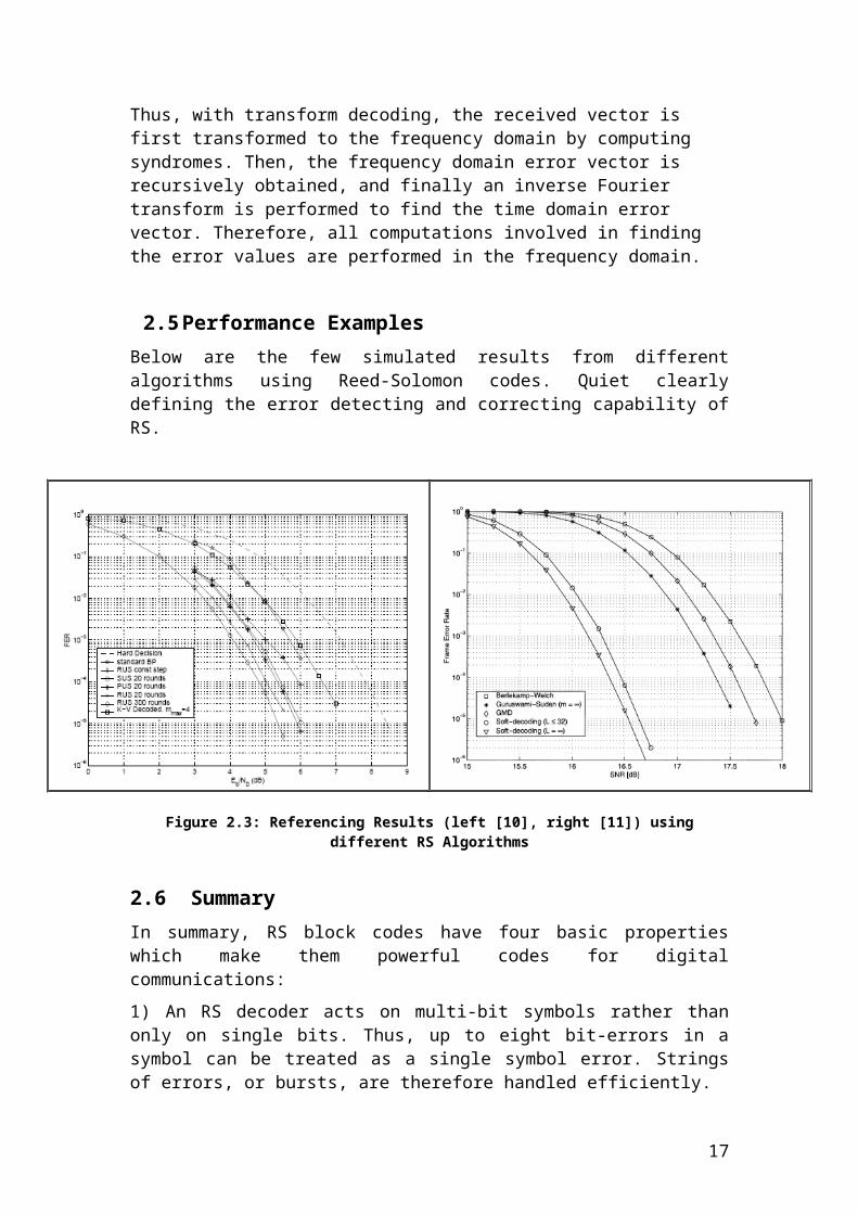
2.5 Performance Examples

Below are the few simulated results from different algorithms using Reed-Solomon codes. Quiet clearly defining the error detecting and correcting capability of RS.

11

Figure 2.3: Referencing Results (left [10], right [11]) using different RS Algorithms

2.6 Summary

In summary, RS block codes have four basic properties which make them powerful codes for digital communications:

1) An RS decoder acts on multi-bit symbols rather than only on single bits. Thus, up to eight bit-errors in a symbol can be treated as a single symbol error. Strings of errors, or bursts, are therefore handled efficiently.

2) The RS codes with very long block lengths tend to average out the random errors and make block codes suitable for use in random error correction.

3) RS codes are well-matched for the messages in a block format, especially when the message block length and the code block length are matched.

4) The complexity of the decoder can be decreased as the code block length increases and the redundancy overhead decreases.

Hence, RS codes are typically large block length, high code rate, codes. [8]

2.6.1 Coding Gain

The advantage of using Reed-Solomon codes is that the probability of an error remaining in the decoded data is (usually) much lower than the probability of an error if Reed-Solomon is not used. This is often described as coding gain.

Example: A digital communication system is designed to operate at a Bit Error Ratio (BER) of 10-9, i.e. no more than 1 in 109 bits are received in error. This can be achieved by boosting the power of the transmitter or by adding Reed-Solomon (or another type of Forward Error Correction). Reed-Solomon allows the system to achieve this target BER with a lower transmitter output power. The power "saving" given by Reed-Solomon (in decibels) is the coding gain.

12

3. Soft In Soft Out DecodingDescription

All the error –correcting algorithm developed so far are based on hard decision in & out puts of the matched filter in the receiver demodulator.

Then, the decoder processes this hard-decision received sequence based on a specific decoding method.

If the outputs of the matched filter are unquantized or quantized in more than two levels, the demodulator makes soft decisions. A sequence of soft-decision outputs of the matched filter is referred to as a soft-decision received sequence. Because the decoder uses the additional information contained in the unquantized received samples to recover the transmitted codeword soft-decision decoding provides better error performance than hard-decision decoding.

Soft Algorithm Classification

Many soft-decision decoding algorithm have been devised.

These decoding algorithms can be classified into two major-categories.

Reliability-Based (or probabilistic) decoding algorithms & code structure-based decoding algorithms.

3.2.1 Reliability-Based Decoding

Reliability-based decoding algorithms generally require generation of a list of candidate code words of a predetermined size to restrict the search space for finding maximum likelihood codeword.

These candidate codeword is generated serially one at a time. Each time a candidate codeword is generated, its metric is computed for comparison & final decoding.

3.2.2 Structure-Based Decoding

13

The most well known structure-based decoding algorithm is the Viterbi algorithm, which is devised based on the trellis representation of a code. This project based on this type of soft in soft out decoding but instead of using typical trellis structure, a new algorithm [1] based on Vardy & Be’ery Decomposition Factor graph.

4. Implementation Of Soft Decoding

4.1 Implementation Goals

On many communication channels errors occur neither independently at random nor in well-defined single bursts but in a mixed manner. Random-error-correcting codes or single-burst-error-correcting codes will be either inefficient or in adequate in combating these mixed errors. Consequently, it is desirable to design codes that are desirable of correcting random errors and/or single or multiple error bursts and give a better performance compared to modulated signal. [7]

As for achieving Reed-Solomon codes efficiency, soft in soft out decoding has been simulated. The algorithm used for reference was

Vardy and Be’ery’s ‘Soft-In Soft-Out Decoding of Reed- Solomon Codes Based on Decomposition [1].

4.2 Overall Architecture

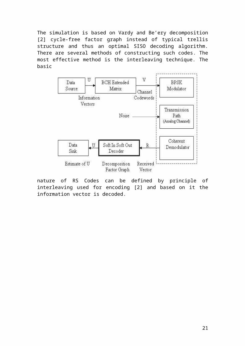
The simulation is based on Vardy and Be’ery decomposition [2] cycle-free factor graph instead of typical trellis structure and thus an optimal SISO decoding algorithm. There are several methods of constructing such codes. The most effective method is the interleaving technique. The basic nature of RS Codes can be defined by principle of interleaving used for encoding [2] and based on it the information vector is decoded.

14

Figure 4. 1: Model of a Coded Digital Communication System

4.2.1 RS Interleaving Nature

Interleaving is another tool used by the code designer to match the error correcting capabilities of the code to the error characteristics of the channel. Interleaving in a digital communications systems enhances the random-error correcting capabilities of a code. [7]

The interleaver subsystem rearranges the encoded bits over a span of several block lengths. The amount of error protection, based on the length of bursts encountered on the channel, determines the span length of the interleaver. The receiver must be given the details of the bit arrangement so the bit stream can be de-interleaved before it is decoded. The overall effect of interleaving is to spread out the effects of long bursts so they appear to the decoder as independent random bit errors or shorter more manageable burst errors.

By interleaving a t-random-error-correcting (n, k) code to degree λ, obtain a (λn, λk) code capable of correcting any combination of t bursts of length λ or less. In the same sense the (n, k) code of RS is spreaded out by (mN, mK) code length

where N<= n and K<= k and m is the bits rate per symbol.

In that sense that if original input information vector after encoding with addition to parity bits is C={v0,…….,vn-1) then after spreading effect to would be in such form C={vo

0,…..,vm-10, vo

1,…..,vm-11,……. vo

n-1,…..,vm-1n-1

}. This is then further processed to noise channel and later passed into decoding stage.

4.3 Technique Applied

The technique mainly used in decoding based on the reference algorithm[1] was to first encode and later decode by factor graph instead of trellis structure. The information bits are encoded by using the BCH extended matrix [2].

Structure Of The Generator Matrix

Let R (N, K) be the Reed-Solomon code over GF (2m) of length N=2m-1 and dimension K. Assume that R is used on a binary channel. Hence, the encoder must employ some fixed linear mapping ø: GF(2m)N –› GF(2)mN to convert a sequence of N elements of GF(2m) into string of mN binary digits. Now let α be a primitive element of GF(2m) and let αS, αS+1,….αS+N-K-1 and their cyclotomic conjugate over GF(2) employed for the linear mapping ø. Defining the codes B1, B2, ….. , Bm

As Bj = {(γjbo, γjb1, γj bN-1) | b= (b0, b1,…, bn-1) Є B (19)

For j=1, 2, ….., m

15

Where, bi Є GF(2) and product γjbi is in GF(2m). B is a subfield subcode of R and, hence , the m codes defined (1) are also subcodes of R. Therefore if (vi

1,…….,vkj) is a

set of k generators for Bj and the set is

j=1Ųm {ø(v1j), ø(v2

j ), ……., ø(vkj )} ( 20)

as the first mk rows of a binary generator matrix for R. By rearranging the columns the structure of Fig.1 is obtained.

4.3.2 Encoding

After implementing the structure for matrix the information vector is multiplied with BCH extended matrix and generating an encoded data with addition to parity bits. In next step interleave the encoded bits. Such as if the encoded bits are n then after interleaving the bits length would become n*rate. Transmission of the signal is randomizing, therefore randomizing the error distribution by applying interleaving. Rate is the square of the minimum hamming distance between two codewords. It specifics the duration or span of the channel memory, not its exact statistical characterization, which is used as time diversity or interleaving. The idea behind interleaving is to separate the codeword symbol in the time. Separating the symbols in time effectively transforms a channel with memory to a memory less one, and thereby enables the random-error-correcting codes to be useful in a burst-noise channel.

Figure 4.2: Structure of the Generator Matrix of the binary image of Crs where B generates Cbch.

16

Figure 4.3: BCH Extended Matrix Structure

4.3.2 RS Factor Graph:

The generator matrix structure seen in Figure.4.2 implies a cycle-free factor graph for RS codes. The RS factor graph consists of m parallel n-stage binary trellis and an additional glue node illustrated in Figure.4.4, where variables are represented by circular vertices, states variables by double circles, and local constraints by using wolf method [3]. The final trellis stage is 2n-k’-ary variable node corresponding to the cosets, or equivalently the syndromes, of CBCH. The node connecting the final trellis stages corresponds to the glue code. The coded bits are labelled {ci

(j)}i=0,….n-1; j=1,…..m and uncoded bits are similarly labelled {a i

(j)} i=0,….k-1; j=1,….m. If there is no priori soft information on uncoded bits and if a systematic encoder is used then the equality constraints in the corresponding sections of the factor graph are enforce ai

(j) = ci

(j) for i=0,….k-1 and j=1,…….,m. Using the factor graph shown in fig.2 the following (nonunique) message-passing schedule ensures optimal SISO decoding.

17

Figure 4.4: RS Code Factor Graph based on the Vardy-Be'ery Decomposition

As the other common structure of trellis gets very complexed with the Reed Solomon interleaving nature, this factor graph simplifies the structure of the decoding. Each 1…m part of the encoded bits are separately sent into 1….m branch of the graph respectively. The result from each branch for example B1……Bm are generated after passing through the trellis and by using soft information the best resultant decoded bits vector is taken by using equation 21.

Cj = B1(j-1) B2

(j-1) ...... Bm(j-1) (21)

Where j=0,......k-1.

18

5. Performance Measures5.1 AWGN channel

In comparing error performance, Additive White Gaussian noise (AWGN) channel was used. The AWGN channel is not always representative of the performance for real channels particular for radio transmission where fading and nonlinearities tend to dominate. Nevertheless, error performance for the AWGN channel is easy to derive and serves as a useful benchmark in performance comparisons.

The error performance is a function of the signal-to-noise (S/N) ratio. Out of the many definitions possible for S/N, the one most suitable for comparison of decoding techniques is the ratio of energy, Eb, to noise density (No). To arrive at this definition and to obtain an appreciation for its usefulness let relate definitions for S/N and Eb/No. The noise source is assumed Gaussian-distributed

The effectiveness of the coding scheme is measured in terms of the Coding gain, which is the difference of the SNR levels of the uncoded and coded systems required to reach the same BER levels.

5.2 Simulation Results

The variation of bit error rate with the Eb/No ratio of a primitive Reed-Solomon code with coherent BPSK signals & Vardy & Be’ery algorithm decoding for AWGN channels has been measured by computer simulations.

Figure 5.1: Simulation result for comparison within (15, 13, 4), (7, 5, 4) RS codes

19

Figure 5.2: Performance of Reed-Solomon codes with Vardy-Be'ery Algorithm decoding in AWGN Channel

Comparisons are made between the coded & uncoded coherent BPSK systems. At high Eb/No ratio, it can be see that the performance of the coded BPSK system is better than the uncoded BPSK systems. At a bit error rate of 10-4 the (15, 13, 4) double-error-correcting Reed-Solomon coded BPSK systems give nearly 3db of coding gain over the uncoded BPSK systems respectively.

The results were generated for 1000 iteration in C code by passing through Gaussian noise on rate 0.5.

5.2.1 Complexity:

Above from the result Figure 5.1 it can be seen that coding gain increases as the rate of the code decreases. Unfortunately, so does the computational complexity of the algorithm. The algorithm has high complexity as it has to search n length codewords for m times (2m(n-k)).

6. Future ResearchesError-control coding covers a large class of codes & decoding techniques. New error-control codes & decoding methods are the result of ongoing research activities in digital communications. After the discovery of Reed-Solomon codes, a search began

20

for an efficient decoding algorithm. None of the standard techniques used at the time were very helpful.

A number of researches are going on for a better db gain over uncoded , hard-decision and other soft decoding algorithms. The aim is not letting get waste the soft information when a signal faces the noise channel. The commercial world is becoming increasingly mobile, while simultaneously demanding reliable, rapid access to sales, marketing and accounting information. Unfortunately the mobile channel is a nasty environment in which to communicate, with deep fades an ever present phenomenon. Reed-Solomon codes are the single best solution; there is no other error control system that can match their reliability performance in the mobile environment. Shot noise and a dispersive, noisy medium plague line-of-sight optical systems, creating noise bursts that are best handled by Reed-Solomon codes. Reed Solomon codes will continue to be used to force communication system performance ever closer to the line drawn by Shannon.

7. Conclusion

This dissertation was based on Vardy and Be’ery Decomposition Algorithm [1], for reducing the complexity of decoding Reed Solomon codes by using soft information through factor graph. The plot clearly shows a nearly 3 db gain over uncoded BPSK signal when comparison is done with RS(15,13,4) and Uncoded(15) code rate.

The Soft-In Soft-out Decoding Of Reed-Solomon Codes Based on Vardy and Be’ery Decomposition Computing [1] is soft-decision decoding algorithm for Reed Solomon codes that incorporate soft-decisions into algebraic decoding framework.

The soft-decision front end can be implemented with a reasonable complexity using the proposed algorithm [1]. Presented simulation results to characterize the coding gains possible from the soft-decision Vardy & Be’ery algorithm for Reed-Solomon codes.

The Vardy & Be’ery algorithm exhibits a performance-complexity tradeoff which is tuneable by the choice of Mmax, n & k.

References

[1] Thomas R. Halford, (Student Member, IEEE.), Vishankan Ponnampalam, (Member, IEEE), Alex J. Grant, (Senior Member, IEEE.), and Keith M. Chugg, (Member, IEEE). Soft-In Soft-out Decoding Of Reed-Solomon Codes Based on

21

Vardy and Be’ery Decomposition Computing. IEEE Transactions on Information Theory, Vol. -51, No. 12, December 2005.

[2] Alexander Vardy (Member, IEEE) and Yair Be’ery (Member, IEEE.), Bit Level Soft-Decision decoding Of Reed-Solomon Codes. IEEE Transactions on Information Theory, Vol. 39, No. 3, January 1991.

[3] Jack K.Wolf, (Fellow, IEEE), “Efficient Maximum Likelihood Decoding Of Linear Block Codes Using a Trellis” IEEE Transactions on Information Theory, Vol. IT-24, No. 1, January 1978.

[4] L.H.Charles Lee. “Error-Control Block Codes, For Communications Engineers”, Artech House, INC, 2000. ISBN 1-58053-032-X

[5] Wikipedia, The free Encylcopedia, Category: “Reed-Solomon Error Correction”.

http://en.wikipedia.org/wiki/Reed_Solomon

Date accessed 21-08-2006.

[6] Turbo Code: “BCH Extended Matrix Structure”.

http://www-sc.enst-bretagne.fr/btc.html

Date accessed 21-08-2006.

[7] Stephen B. Wicker. “Error Control Systems, For Digital Communication and Storage”, Prentice-Hall, Inc, 1995. ISBN 0-13-200809-2

[8] Bernard Sklar. “Digital Communications: Fundamentals and applications (2nd,ed)”, Prentice-Hall, Inc, 2001. ISBN 0-13-084788-7

[9] Wicker Bhargava. “Reed Solomon Codes and Their Applications”, IEEE PRESS Marketing © 1994 ISBN 0-7803-1025-X

[10] Jing Jiang, Student Member, IEEE and Krishna R. Narayanan, Member, IEEE “Iterative Soft Decoding of Reed Solomon Codes” Department of Electrical Engineering, Texas A&M University, College Station, USA

[11] Ralf Koetter, Member, IEEE, and Alexander Vardy, Fellow, IEEE “Algebraic Soft-Decision Decoding of Reed–Solomon Codes”

22

23