Estimating the Intergenerational Elasticity and Rank Association in the US:

Overcoming the Current Limitations of Tax Data

Bhashkar Mazumder*

Federal Reserve Bank of Chicago

April, 2015

Abstract:

Ideal estimates of the intergenerational elasticity (IGE) in income require a large panel of income

data covering the entire working lifetimes for two generations. Previous studies have

demonstrated that using short panels and covering only certain portions of the lifecycle can lead

to considerable bias. A recent influential study by Chetty et al (2014) using tax data, estimates

the IGE in family income for the entire U.S. to be 0.344, considerably lower than most previous

estimates. Despite the seeming advantages of extremely large samples of administrative tax

data, I demonstrate that the age structure and limited panel dimension of the data used by Chetty

et al leads to considerable downward bias in estimating the IGE. Specifically I use PSID

samples that overcome the data limitations in the tax data to estimate the IGE when using long

time averages centered around age 40 in both generations. I demonstrate how imposing the data

limitations in Chetty et al (2014) lead to considerable downward bias relative to these preferred

estimates. I further demonstrate that the sensitivity checks in Chetty et al regarding the age at

which children’s income is measured and the length of the time average of parent income used to

estimate the IGE, are also flawed due to these data limitations. The lack of robustness of the IGE

to the treatment of years of zero earnings among children found by Chetty et al is also largely

due to data limitations . Estimates of the rank-rank slope on the other hand are much less

downward biased and tend to be more robust to the limitations of the tax data. Nevertheless,

researchers should continue to use both the IGE and rank based measures depending on which

concept of mobility they wish to address. Substantively, I find that the IGE in family income in

the U.S. is likely greater than 0.6 and that the rank-rank slope is 0.4 or higher.

*I thank Andy Jordan for outstanding research assistance. The views expressed here do not

reflect those of the Federal Reserve Bank of Chicago or the Federal Reserve system.

2

I. Introduction

Inequality of opportunity has become a tremendously salient issue for policy makers

across many countries in recent years. The sharp rise in inequality has given rise to fears that

economic disparities will persist into future generations. This has resulted in a heightened focus

on the literature on intergenerational economic mobility. This body of research which is now

several decades old seeks to understand the degree to which economic status is transmitted

across generations. Of course, a critical first step in understanding this literature and correctly

interpreting its findings is having a sound understanding of the measures that are being used and

what they do and do not measure. This paper will focus on two prominent measures of

intergenerational mobility: the intergenerational elasticity (IGE) and the rank-rank slope and

discuss several key conceptual and measurement issues related to these estimators in the context

of the U.S.

The IGE has a fairly long history of use in economics dating back to papers from the

1980s. It is generally viewed as a useful and transparent summary statistic capturing the rate of

“regression to the mean”. It can for example, tell us how many generations (on average) it

would take the descendants of a family to rise to the mean level of income. In recent years many

notable advances have been made in terms of measurement and issues concerning life-cycle bias

(e.g. Jenkins, 1987; Solon, 1992; Mazumder, 2005a; Grawe, 2006; Böhlmark and Lindquist,

2006; Haider and Solon, 2006).1 As a result of these contributions, most recent US estimates of

the IGE in family income are generally around 0.5 or higher.2 In a recent highly influential study

1 Reviews of this literature can be found in Solon (1999) and Black and Devereaux (2011).

2 Solon (1992) estimates the IGE in family income to be 0.483 (Table 4). Hertz (2005) reports an elasticity in age

adjusted family income of 0.538. Hertz (2006) estimates the IGE in family income to be 0.58 and the IGE in family income per person to be 0.52. Bratsberg et al (2007) produce an estimate of the elasticity of family income on earnings of 0.54. Jantti et al (2006) produce an estimate of the same elasticity of 0.517. In making comparisons

3

Chetty et al (2014) use large samples drawn from IRS tax records produce estimates of the IGE

in family income of just 0.344. As I show below, such an estimate paints a dramatically different

view of the rate at which a family can expect to escape poverty. The main focus of Chetty et al

(2014) is not their national IGE estimates. Instead Chetty et al are the first to produce estimates

of mobility at a very detailed level of U.S. geography and to provide evidence of substantial

heterogeneity across the U.S. Nevertheless, Chetty et al make strong claims about their tax their

IGE estimates, arguing that none of the previous biases in the literature apply to their data.

Given the importance of the IGE as one of the key conceptual measures of intergenerational

mobility, it is worth revisiting the issues concerning measurement and life-cycle bias in the

context of their sample.

A key point of this paper is to demonstrate that despite having extremely large sample

sizes, the IRS-based intergenerational sample used by Chetty et al is fundamentally limited in a

few key respects stemming from the fact that the data is only available going back to 1996. First,

children’s income is only measured in 2011 and 2012. This is at a relatively early point in the

life cycle for cohorts born between 1980 and 1982 and at a time in which unemployment was

quite high in the US. Even setting aside business cycle effects, this is an age at which we would

expect substantial life cycle bias based on the estimates from the prior literature (Haider and

Solon, 2006). Moreover, relative to an ideal data structure, where cohorts of children could be

chosen such that they were observed over the 31 years spanning the ages of 25 to 55, Chetty et al

are limited to using only 6 percent of the lifecycle. Second, parents’ income is also measured for

only a short period (5 years) covering just 16 percent of the lifecycle and at a relatively late

period in life. I estimate that about 25% of observations of fathers’ income in their sample are

with Chetty et al (2014) it is important to distinguish these estimates from those that use a different income concept such as labor market earnings in both generations.

4

measured at age 50 or higher. The prior literature has shown that the transitory fluctuations in

income comprise a substantial share of the variance in parent income around the age of 50 also

attenuating the estimate of the IGE relative to what would be found if one used lifetime income

(Haider and Solon, 2006; Mazumder, 2005a). Third, recent research has established that

administrative data can lead to worse measurement error than survey data, particularly at the

bottom end of the income distribution (e.g. Abowd and Stinson, 2013 and Hokayem et al., 2012,

2015).

I use the PSID which covers income going back to 1967 to demonstrate the implications

of these data limitations, empirically. First, I construct an intergenerational sample where both

kids and parents family income is observed over a vastly larger portion of the lifecycle than the

IRS records and where crucially, the time averages are centered over the prime working years in

both generations. I estimate the IGE using this closer to “ideal” sample and then show how the

estimates change if I impose the same kinds of data limitations that exist in the IRS data. The

results of this exercise show that the data limitations lead to IGE estimates that are about 60

percent of the size of the estimates with the complete data and similar in magnitude to the

estimates of Chetty et al.

Chetty et al. also find that with their tax data the IGE estimates are very sensitive to how

they choose to impute the income of children who report no family income during 2011 and

2012. This apparent sensitivity of the IGE estimates is also due in large part to the limitations of

the tax data that is currently available rather than an intrinsic feature of the estimator. The

critical issue is that it is the limited panel dimension of the tax data that makes the analysis

especially sensitive to this problem. This is also important because it is this concern about

robustness of the IGE with their particular sample that is a primary reason that Chetty et al turn

5

to rank-based estimators.3 This can be contrasted with several other studies (Bhattacharya and

Mazumder, 2011; Corak et al., 2014; Mazumder, 2014; Davis and Mazumder, 2015; and

Bratberg et al., 2015), that have also used rank-based measures to study intergenerational

mobility but for conceptual reasons.

Given the recent shift in the literature to using rank-based measures it is useful to

distinguish the measurement concerns with the IGE from the conceptual differences between the

two estimators. In short, I argue that conceptually, both measures can provide useful insights

about different aspects of mobility. I argue that there are clearly certain questions that are best

answered by the IGE and for that reason researchers should continue to use the IGE as at least

one tool for measuring intergenerational mobility. Nevertheless, rank-based estimators are also

valuable because in addition to providing information on a different concept of mobility,

positional mobility, rank-based measures are also useful for distinguishing upward versus

downward movements, making subgroup comparisons and for identifying nonlinearities in

intergenerational mobility. In fact, I would argue that even if Chetty et al found the IGE to be

perfectly robust in their tax data, that it would still be preferable to use rank-mobilty measures to

understand geographic differences. This is because an IGE estimated in say, Charlotte, North

Carolina would only be informative about the rate of regression to the mean income in Charlotte

whereas rank estimators can use ranks that are fixed to the national distribution which may make

for a more meaningful comparison across cities.

Perhaps the most significant contribution of the paper is to show that the magnitude of

the IGE estimates when using many years of income data centered over the prime working years

in both generations are higher than almost all previous estimates in the literature. For example,

3 Dahl and Deliere (2009) also shift to rank based measures based on concerns regarding the robustness of the iGE

but their concerns revolve around a different measurement issue than Chetty et al. I discuss the problems with Dahl and Deliere’s analysis in footnote 14 in section 3.

6

the estimates of the IGE with respect to family income are greater than 0.6. Turning to a

different measure of income, the labor income of male heads of household, I also find that the

IGE is greater than 0.6 and roughly similar to the estimate found by Mazumder (2005a) using

social security earnings data. Chetty et al suggest that the high estimates in Mazumder (2005a)

are due to data imputations of fathers earnings that are topcoded in some years. The analysis

here suggests that those earlier findings can easily be replicated using publicly available survey

data that requires no imputations of topcoded earnings whatsoever. Instead, obtaining such high

estimates of the IGE simply requires using samples with the appropriate ages and long time

spans of available income data centered around the prime working ages in both generations. I

also point to other studies in the literature that yield findings consistent with Mazumder (2005a)

that do not require imputations (e.g. Mazumder, 2005b; Nilsen et al (2012); and Mazumder and

Acosta, 2014).

A final exercise uses the PSID data to estimate the rank-rank slope which is one of the

two main measures used by Chetty et al (2014). In this case the estimates are only moderately

larger with the PSID (0.4 or higher) than what one obtains when using the IRS data (0.341) or

the PSID data when imposing the age structure and short panels found in the tax data. This

suggests that while the rank-rank slope may be more robust to the data limitations of the IRS

sample than the IGE, it is still not perfect and suggests that the rate of intergenerational mobility

even by rank-based measures may be overstated by the tax data. These pattern of results are

broadly in line with similar findings for Sweden (Nybom and Stuhler, 2015).

One clear conclusion to be drawn from this paper is that researchers should continue to

use the IGE if that is the conceptual parameter of interest and when their intergenerational

samples have the appropriate panel lengths and age structure. Even when the ideal data is not

7

available, researchers can still attempt to assess the extent of the bias based on prior papers in the

literature that propose methodological fixes. Substantively, the results of this paper show that

intergenerational mobility in the US is substantially lower than what one would think based on

using the currently available IRS data especially if one is interested in the rate at which income

gaps between families are closed. If one is more interested in purely positional mobility then the

bias due to the data limitations in the tax data is less severe. Over the next few decades, as the

panel length of the tax data increases, these biases will recede in importance. However, one

cannot know with certainty whether researchers will be able to obtain such tax data in future

decades.

The rest of the paper proceeds as follows. Section 2 describes the conceptual differences

between the estimators. Section 3 describes measurement issues with IGE estimation and

describes the structure of an “ideal” dataset. It then compares this ideal dataset with the IRS-

based intergenerational sample used by Chetty et al (2014) and a close to ideal sample that can

be constructed with publicly available PSID survey data. Section 4 outlines the PSID data used

for the analysis. Section 5 presents the main results when using the PSID and demonstrates the

effects of imposing the limitations with the tax data. Section 6 concludes.

II. Conceptual Issues

The concept of regression to the mean over generations has a long and notable tradition

going back to the Victorian era social scientist Sir Francis Galton who studied among other

things the rate of regression to the mean in height between parents and children. Modern social

scientists have continued to find this concept insightful as a way of describing the rate of

intergenerational persistence in a particular outcome and to infer the rate of mobility as the flip

8

side of persistence. In particular economists have focused on the intergenerational elasticity

(IGE). The IGE is the estimate of obtained from the following regression:

(1) y1i = + y0i + i

where y1i is the log income of the child generation and y0i is the log of income in the parent

generation.4 The estimate of provides a measure of intergenerational persistence and 1 - can

be used as a measure of mobility. One way to interpret the elasticity in practical terms is to

consider what it implies about how many generations it would take for a family living in poverty

to attain close to the national average household income level. If for example, the IGE is around

0.60 as claimed by Mazumder (2005a) then it would take 6 generations (150 years). On the

other hand if the IGE is around 0.34 as claimed by Chetty et al (2014) then it would take just 3

generations.5 Clearly, the two estimates have profoundly different implications on the rate of

intergenerational mobility and if the rate of regression to the mean is what we are interested in

knowing then the IGE is what we ought to estimate. The concept of regression to the mean is

also widely used in other aspects of economics such as the macroeconomic literature on

differences in per-capita income across countries (e.g. Barro and Sala-i-Martin, 1992).

The rank–rank slope on the other hand is about a different concept of mobility, namely

positional mobility. For example, a rank-rank slope of 0.4 suggests that the expected difference

in ranks between the adult children of two different families would be about 4 percentiles if the

difference in ranks among their parents was 10 percentiles. One can imagine that depending on

the shape of the income distribution the descendants of a family in poverty might experience

4 Often the regression will include age controls but few other covariates since is not given a causal interpretation

but rather reflects all factors correlated with parent income 5 This exercise is based on Mazumder (2005) and considers a family of four with two children under the age of 18

whose income is $18,000 (under the poverty threshold in 2013 of around $24,000). Mean household income in 2013 was approximately $73,000. The calculation specifically examines how many generations before the expected income of the descendants of this family would be within 5% of the national average.

9

relatively rapid positional mobility but slower regression to the mean.6 How are the two

measures related? Chetty et al (2014) point out that that the rank-rank slope is very closely

related to the intergenerational correlation (IGC) in log income. They and many others have also

shown that the IGE is equal to the IGC times the ratio of the standard deviation of log income in

the child generation to the standard deviation of log income in the parent generation:

(2)

This relationship is sometimes taken to imply that a rise in inequality would lead the IGE

to rise but not affect the IGC and that therefore, the IGC may be a preferred measure that avoids

a “mechanical” effect of inequality. By extension one might also prefer the rank-rank slope if

one accepts this argument. Several comments are worth making here. First, in reality the

parameters are all jointly determined by various economic forces. In the absence of a structural

model one cannot meaningfully talk about holding “inequality” fixed. For example, a change in

might cause inequality to rise, rather than the reverse, or both might be altered by some third

force such as rising returns to skill. The mathematical relationship shown in (2) does not

substitute for a behavioral relationship and so it does not make sense to pretend that we can

separately isolate inequality from the IGE. Second, even if it was the case that the IGC or rank-

rank slope was a measure that was “independent of inequality”, that doesn’t mean that society

shouldn’t continue to be interested in the rate of regression to the mean. I would argue that it is

precisely because of the rise in inequality that societies are increasingly concerned about

intergenerational persistence and so incorporating the effects of inequality may actually be

critical to understanding the rates of mobility that policy makers want to address.

6 In the example above, one can imagine that it may take significantly longer for the family with income of $18,000

to attain the mean income level of $73,000 than the median income level of $52,000.

10

In addition to providing useful information about positional mobility the rank-rank slope

has other attractive features. Perhaps it’s most useful advantage over the IGE is that it can be

used to measure mobility differences across subgroups of the population with respect to the

national distribution. This is because the IGE estimated within groups is only informative about

persistence or mobility with respect to the group specific mean whereas the rank-rank slope can

be estimated based on ranks calculated based on the national distribution. Chetty et al (2014)

were able to use this to characterize mobility for the first time at an incredibly fine geographic

level. Mazumder (2014) used other “directional” rank mobility measures to compare racial

differences in intergenerational mobility between blacks and whites in the U.S. However, for

characterizing intergenerational mobility at the national level both the IGE and the rank-rank

slope are suitable depending on which concept of mobility the researcher is interested in

studying.

III. Measurement Issues and the Ideal Intergenerational Sample

Measurement Issues

The prior literature on intergenerational mobility has highlighted two key measurement

concerns that I will briefly review here. The first issue is attenuation bias that arises from

measurement error or transitory fluctuations in parent income. In an ideal setting the measures

of y1 and y0 in equation (1) would be measures of lifetime or permanent income but in most

datasets we only have short snapshots of income that can contain noise and attenuate estimates of

the IGE. Solon (1992) showed that using a single year of income as a proxy for lifetime income

of fathers can lead to considerable bias relative to using a 5 year average of income. Using the

PSID, Solon concluded that the IGE in annual labor market earnings was 0.4 “or higher”.

Mazumder (2005a) used the SIPP matched to social security earnings records and showed that

11

using even a 5-year average can lead to considerable bias and estimated the IGE in labor market

earnings to be around 0.6 when using longer time averages of fathers earnings (up to 16 years).

Mazumder argues that the key reason that a 5-year average is insufficient is that the transitory

variance in earnings tends to be highly persistent and appeals to the findings of U.S. studies of

earnings dynamics that support this point. Using simulations based on parameters from these

other studies, Mazumder shows that the attenuation bias from using a 5-year average in the data

is close to what one would expect to find based on the simulations. In a separate paper, that is

less well known, Mazumder (2005b) showed that if one uses short term averages in the PSID and

uses a Hetereoscedastic Errors in Variables (HEIV) estimator that adjusts for the amount of

measurement error or transitory variance contained in each observation, then that the PSID

adjusted estimate of the IGE is also around 0.6. This latter paper is a useful complement because

unlike the social security earnings data used by Mazumder (2005a) the PSID data is not topcoded

and doesn’t require imputations. Chetty et al (2014) has contended that the larger estimates of the

IGE in Mazumder (2005a) were due to the nature of the imputation process rather than due to

larger time averages of fathers’ earnings. I will return to this point below and show that the

evidence from the PSID suggests that their contention is incorrect.

The second critical measurement concern in the literature concerns lifecycle bias best

encapsulated by Haider and Solon (2006). One aspect of this critique concerns the effects of

measuring children’s income when they are too young. Children who end up having high

lifetime income often have steeper income trajectories than children who have lower lifetime

incomes. Therefore if income is measured at too young an age it can lead to an attenuated

estimate of the IGE. Haider and Solon show that this bias can be considerable and is minimized

when income is measured at around age 40. A related issue is that transitory fluctuations are not

12

constant over the lifecycle but instead follow a u-shaped pattern over the lifecycle (Baker and

Solon, 2003; Mazumder, 2005a). This implies that measuring parent income when they are

either too young or (especially) when they are too old can also attenuate estimates of the IGE.

While there are econometric approaches one can use to correct for lifecycle bias, one simple

approach would be to simply center the time averages of both children’s and parents income

around the age of 40. Using this approach with the PSID, Mazumder and Acosta estimate the

IGE to be around 0.6. Further, Nilson et al (2012), using Norweigian data show that both time

averaging and life-cycle bias play a role in attenuating IGE coefficients. It should be noted that

Nilsen et al find that these biases matters despite using administrative data like Chetty et al.7

Comparisons of Intergenerational Samples

To better understand the limitations with currently available intergenerational samples in

the US with respect to these measurement issues, it is useful to think about what an ideal sample

would look like. In an ideal setting we would want to construct an intergenerational sample

where income is measured for both generations throughout the entire working life cycle, say

between the ages of 25 and 55.8 For example, suppose our data ends in 2012 (as in Chetty et al)

then for full lifecycle coverage for the children’s generation we would want cohorts of children

who were born in 1957 or earlier. For the 1957 cohort we would measure their income between

1982 and 2012. For the 1956 cohort we would measure income between 1981 and 2011 and so

on. Suppose that for the parent generation, the mean age at the time the child is born is 25. Then

for the 1957 cohort we would collect income data from 1957 to 1987 and from 1956 to 1986 for

the parents of the earlier birth cohorts, and so on. With such a dataset in hand we would be

7 Chetty et al speculate that perhaps time averaging and life cycle bias don’t matter because of their use of

administrative data. 8 The precise end points are debatable but one might want to ensure that most sample members have finished

schooling and that most sample members have not yet retired.

13

confident that we would have measures of lifetime income that are error-free and would also be

free of lifecycle bias.

Unfortunately, for most countries, including the US, it is difficult to construct an

intergenerational dataset with income data going back to the 1950s.9 Still, we can come

somewhat close to this ideal sample with publicly available survey data in the Panel Study of

Income Dynamics (PSID). The PSID began in 1968 and started collecting income data

beginning with 1967 for a nationally representative sample of about 5000 families. The 1957

cohort would have been 11 years old at the time the PSID began so this cohort along with those

born as early as 1951 would have been under the age of 18 at the beginning of the survey. The

approach I take in this paper is to construct time averages of both parent and child income

centered around the age of 40 in order to minimize life-cycle bias. For parents, these time

averages include income obtained between the ages of 25 and 55 and for children these averages

include income obtained between the ages of 35 and 45.

Relative to the ideal sample, the PSID sample is close in several regards. Since it covers

the 1967 to 2010 period it is able cover utilize large windows of the lifecycle for both

generations. For example, for the 16 cohorts born between 1951 and 1965, in principle, income

can be measured in all years that cover the age range between 35 and 45. For the cohorts born

between 1967 and 1975, their parent’s income can also be measured through the ages of 25 and

55. Of course, attrition from the survey can diminish the size of samples with observations in all

9 The SIPP-SER data used by Mazumder (2005) and Dahl and Deliere (2008) meets some but not all of these

requirements.

14

of these years but unlike with the currently available tax data, the potential for such coverage is

there.10

Now let us contrast this with the limitations faced by Chetty et al (2014) in their analysis

of currently available IRS data. First the tax data is currently only digitized going back to 1996,

which is nowhere near as far back as the ideal dataset would require (1957), or even what is

available in the PSID (1967). Therefore, there is no birth cohort for whom the income of parents

can be measured for the entire 31 year time span between the ages of 25 and 55. Furthermore,

the authors chose to limit the analysis to just a 5-year average between 1996 and 2000. Although

they do not explain why they limited their time average to just 5 years, a likely explanation is

that if they had extended their time averages further, they would have been forced to measure

income when parents were at an older than ideal age. This will become important later when I

explain why their sensitivity analysis is flawed. The mean age of fathers in their sample in 1996

is reported to be 43.5 with a standard deviation of 6.3 years. This implies that over the 5 years

from 1996 through 2000, roughly 24 percent of the father-year observations used in constructing

the average would be when fathers are over the age of 50.11

This is an age at which the

transitory variance in income is quite high (Mazumder, 2005a). They also report that prior to

1999 they record the income of non-filers to be zero. Therefore for about 3 percent of

observations in three of the five years used in their average they impute zeroes to the missing

observations.12

10

As discussed later, I use survey weights to address concerns about attrition. 11

This example assumes the data is normally distributed. In 2000, more than a third of the observations would be when fathers are over the age of 50. 12

See footnote 14 of Chetty et al. (2014). They show that this has no effect on their rank mobility estimates but they do not show how the IGE estimates change. Further, measuring income from 1999 to 2003 only worsens the attenuation bias in the IGE resulting from measuring fathers at late ages.

15

For the children in the sample, the data limitations are even more severe. Chetty et al use

cohorts born between 1980 and 1982 and measure their income in 2011 and 2012 when they are

between the ages of 29 and 32. For this age range, simulations from Haider and Solon (2006)

suggest that there would be around a 20 percent bias in the estimated IGE compared to having

the full lifecycle. A further complication is that their measures are taken in 2011 and 2012 when

unemployment was relatively high and labor force participation quite low. They report that they

drop about 17 percent of observations from the poorest families due to their having zero income

over those 2 years. If their sample also included 29 to 32 year olds over several decades which

also included many boom years then this would be less of a concern. Finally, there is a concern

about whether administrative income data adequately captures true income, particularly at the

low and the high ends of the income distribution. For example, at the lower end of the

distribution, tax data could miss forms of income that go unreported to the IRS. At the higher

end, tax avoidance behavior could lead to an under-reporting of income. Hoyakem et al (2012,

2015) find that administrative tax data does a worse job than survey data in measuring poverty.

Abowd and Stinson (2013) argue that it is preferable to treat both survey data and administrative

data as containing error. I also discuss below, how a preferred concept of family income that

includes all resources available for consumption, including transfers and income of other family

members would render tax data inadequate.

It is useful to visualize just how different the data structure of the Chetty et al sample is

from an ideal intergenerational sample. This is shown in Figure 1. For each of three samples

there are two columns of 31 cells representing the ages from 25 to 55 in each generation and we

assume that just one parent’s income can be measured. The degree of coverage over the life

course is represented by the extent to which the cells are colored. Panel A shows that if we

16

measured income in both generations using data spanning the entire life course for two

generations then all the cells in both generations would be colored in. Panel B contrasts this with

a typical parent-child observation in the Chetty et al sample.13

This makes it clear just how small

a portion of the ideal lifecycle is covered. Just 6 percent of the child’s lifecycle and just 16

percent of the parent’s lifecycle would be covered. Panel C contrasts this with an example of a

result that will be produced with the PSID in the current study. There are many cohorts for

whom both child and parent income can be measured over several years centered around the age

of 40 when lifecycle bias is minimized. The figure presents an example of a 7-year average of

child income and a 15-year average of parent income. Such a sample would cover 23 percent of

the child’s lifecycle and 48 percent of the parent’s lifecycle.

To their credit, Chetty et al (2014) attempt to conduct some sensitivity checks to these

issues, but for the same reasons discussed above, their data are not well suited to doing effective

robustness checks for the IGE measure. Below I will replicate their sensitivity checks with the

PSID data and show how the current data limitations with the IRS data lead them to erroneous

conclusions regarding the sensitivity of their IGE estimates to these measurement problems.

Is the IGE Robust to Zeroes?

Chetty et al (2014) also argue that the IGE estimator is not robust to how they impute

years of zero family income observed for individuals in the child generation observed in 2011

and 2012.14

They obtain an estimate of 0.344 when they restrict the sample to those children

13

This example takes a child born in 1981 whose income is observed at age 30 and 31 during the years 2011 and 2012. I assume that father was 29 years old when the child was born so that the father’s income is measured between the ages of 44 and 48 during the years 1996 to 2000. This example closely tracks the mean ages of the sample as reported by Chetty et al (2014). 14

It is worth pointing out that this is very different from the robustness issue discussed by Dahl and Deliere (2008) who are worried about years of zero earnings for parents, not kids. Dahl and Deliere utilize social security earnings data. For the years 1951 through 1983, they cannot distinguish between years of zero earnings due to non-

17

with positive income in both years. If they impute $1000 of income to these individuals then

their IGE estimate rises to 0.413. If they assign $1 then their IGE estimate rises to 0.618. There

are two points worth making here. First, this seeming lack of robustness again reflects, at least in

part, the poor lifecycle coverage of their sample. To see why this is the case, imagine a

hypothetical researcher in the year 2035 that attempts an intergenerational analysis for the 1980

birth cohort using the tax data. In 2035 one would have complete information on family income

throughout the ages of 25 to 55 and would not have to worry that some of these individuals

reported no income in 2 of the 31 years of the lifecycle, during a period when unemployment

was relatively high. There would be as many as 29 other years of income data available to

calculate lifetime income. In fact, based on the prior literature, a researcher could probably

obtain a fairly unbiased estimate of the IGE for the 1980 birth cohort by the early 2020s if they

could obtain even a few years of income around the age of 40. In contrast, datasets such as the

PSID covering cohorts born as far back as the 1950s can be observed over many years, at many

ages, and at different stages of the business cycle.

A second point relates to the concept of family income one wants to use. Economists

(e.g. Mulligan, 1997) have sometimes argued that an ideal measure of intergenerational mobility

would seek to measure lifetime consumption in both generations since consumption is perhaps

the measure closest to utility which is what economists focus on. In this case ideally we would

coverage in the SSA sector from true zeroes due to non-employment. When they construct measures of parent average earnings over the ages of 20 to 55 and include all years of zero earnings they obtain estimates of the intergenerational elasticity of around 0.3 for men. Their estimates may be including many years when actual earnings are actually positive but are erroneously treated as zero because fathers were working in the non-covered sector. They attempt to correct for this by restricting the sample to parents who were not in the armed forces, or self-employed in some specifications. But, importantly this is only observed in 1984.and their long-term averages may still include many years of zero earnings for workers who were actually in the non-covered sector in the 1950s, 1960s or 1970s but who had shifted to the covered sector by 1984. When they restrict the number of years of zero earnings in other very sensible ways to directly address the issue, they obtain estimates of around 0.5 to 0.6. For example, when they use the log of average earnings beginning with the first 5 consecutive years of positive earnings up to age 55 they obtain an estimate of 0.498.

18

like to measure total family resources which includes income obtained from transfers and from

other family members. This is an example where survey data that has access to transfer income

would be preferable to tax data that may not. Including transfers may not only be a preferred

measure but may also help alleviate the problem of observing zero earnings or zero income as is

common in administrative data. It is also not obvious why the preferred measure of family

income would be one that only includes labor market earnings, transfers and capital income that

happen to be reported on tax forms.

Overall, there are strong reasons to think that the seeming lack of robustness of the IGE

in Chetty et al is more a problem of limitations with their tax data rather than with the estimator

itself. In fact, the results using broader concepts of family income with the PSID shown below

are virtually identical regardless of whether one includes or doesn’t include years of zero income

since there so few zeroes.

IV. PSID Data

I restrict the analysis to father-son pairs as identified by the PSID’s Family Identification

Mapping System (FIMS) and use all years of available family income between the ages of 25

and 55 between the years of 1967 and 2010. For the main analysis I consider a measure of

family income that excludes transfers and excludes income from household members that are not

the head of household or the spouse. This provides a measure of family income that might be the

most comparable to the concept used by Chetty et al (2014). In addition, I also construct a

measure of family income that also includes transfers received by the household head or spouse

but these results are not shown in this paper. Finally, I construct a measure that uses only the

labor income of the father and son to be more comparable to papers that emphasize the IGE in

labor market income (e.g. Solon, 1992; Mazumder, 2005). Labor income is not simply earnings

19

from an employer but also incorporates self-employment. Observations marked as being

generated by a ‘major’ imputation are set to missing. Yearly income observations are deflated to

real terms using the CPI. In the PSID the household head is recorded as having zero labor

income if their income was actually zero or if their labor income is missing, so one cannot

cleanly distinguish true zeroes with the labor income. All of the main analysis only uses years of

non-zero income when constructing time averages of income. When using family income,

instances of reports of zero income are relatively rare so the results are virtually immune to the

inclusion of zeroes.

The main analysis only uses the nationally representative portion of the PSID and

includes survey weights to account for attrition. All of the analysis was also done including the

SEO oversample of poorer households and also includes survey weights. While the samples

with the SEO are larger and offer more precise estimates, there is some concern about the

sampling methodology (Lee and Solon, 2009). Finally all estimates are clustered on fathers.

The approach to estimation in this study is slightly different than in most previous PSID

studies of intergenerational mobility. Rather than relying on any one fixed length time average

for each generation and relying on parametric assumptions to deal with lifecycle bias (e.g. Lee

and Solon, 2009), instead I estimate an entire matrix of IGE’s for many combinations of lengths

of time averages that are all centered around age 40. I will present the full matrix of estimates

along with weighted averages across entire rows and columns representing the effects of a

particular length of the time average for a given generation. For example, rather than simply

comparing the IGE from using a ten-year average of fathers income to using a five year average

of fathers’ income for one particular time average of sons income, I can show how the estimates

are affected for every time average of sons’ income.

20

V. Results

IGE Estimates

Table 1 shows the estimates of the IGE in family income that is conceptually similar to

that used by Chetty et al (2014). The first entry of the table at the upper left shows the estimate

if we use just one year of income of family income in the parent generation and one year of

family income for the sons when they are closest to age 40 and also are within the age-range

constraints described earlier. This estimate of the IGE is 0.414 with a standard error of (0.075)

and utilizes a sample of 1358. One point immediately worth noting is that this estimate which

uses just a single year of family income around the age 40 is higher than the 0.344 found by

Chetty et al (2014). Moving across the row, the estimates gradually include more years of

income between the ages of 35 and 45 for the sons. At the same time the sample size gradually

diminishes as an increasingly fewer number of sons have will income available for a higher

length of required years. For the most part the estimates don’t change much and most are in the

range of 0.35 and 0.42. At the end of the row I display the weighted average across the columns,

where the estimates are weighted by the sample size. For the first row the weighted average is

0.381.

Moving down the rows for a given column, the estimates gradually increase the time

average used to measure family income in the parent generation and as a consequence also

reduces the sample size. For example, if we move down the first column and continue to just use

the sons’ income in one year measured closet to age 40 and now increase the time average of

fathers’ income to 2 years, the estimate rises to 0.439 as the sample falls to 1317. Using a five

year average raises the estimate to 0.530 (N=1175). Increasing the time average to 10 years

increases the estimate 0.580 (N=895). Using a 15 year average raises the estimate further to

21

0.680 (N=533). The weighted average for each row is displayed in the last column and the

weighted average for each column is displayed in the bottom row.

A few points are worth making. Since expanding the time average in either dimension

reduces the sample size it risks making the sample less representative. The implications on the

estimates, however, are quite different for whether we increase the time average for the sons’

generation or for the fathers. For the parent generation, increasing the time average tends to raise

estimates. This is a consistent with a story in which larger time averages reduce attenuation bias

stemming from mis-measurement of parent income (Solon, 1992; Mazumder, 2005). This also

accords with standard econometric theory concerning mis-measurement of the right hand side

variable. On the other hand, econometric theory posits that mis-measurement in the dependent

variable typically should not cause attenuation bias. Indeed, increasing the time average of sons’

family income has little effect. But crucially, this is because we have centered the time average

of family income in each generation so that the lifecycle bias which induces “non-classical”

measurement error in the dependent variable (Haider and Solon, 2006) may already be accounted

for.

By this reasoning one might consider the estimates in the first column to be the most

useful since they allow one to see how a reduction in measurement error in parent income affects

the estimates while simultaneously minimizing life cycle bias and keeping the sample as large as

possible. A more conservative view would be to use the weighted average in the final column

that takes into account the possible effects of incorporating more years of data on sons’ income

while also giving greater weight to estimates with larger samples. Figure 2 shows the pattern of

estimates from the two approaches as I gradually use longer time averages. Using either

approach suggests that the IGE in family income is greater than 0.6. Appendix Table 1 and

22

Figure 1 show the analogous set of estimates using larger samples that include the SEO

oversample.

The key idea of the study is to see how these IGE estimates would compare to what one

would obtain by imposing the current data limitations of the IRS sample. To do this, one can use

the second column and fifth row of Table 1 as a baseline estimate. That estimate of 0.493 uses a

two year average of family income of sons centered around age 40 and a five year average of

parent income centered around age 40. If I now impose a sample restriction such that I use a two

year average of sons taken over the ages of 29-32 and use a five year average of parent income

centered around the age of 46 then the estimate I obtain is 0.282 (s.e. = 0.099). This is only 57

percent of the value when using similar time averages centered at age 40. Furthermore, if the

true IGE is actually 0.7, then it is only 40 percent of the true parameter. If I include the SEO

subsample then the estimate rises a bit to 0.325 (s.e. = 0.081). For that sample, the data

limitations yield estimates that are 62 percent of the comparable estimates when using time

averages centered at age 40. Neither of the two estimates are statistically different from the

Chetty et al estimate of 0.344. This suggests that it is the data limitations in the tax data that lead

Chetty et al to produce estimates that are vastly lower than what has been reported in most of the

previous literature.

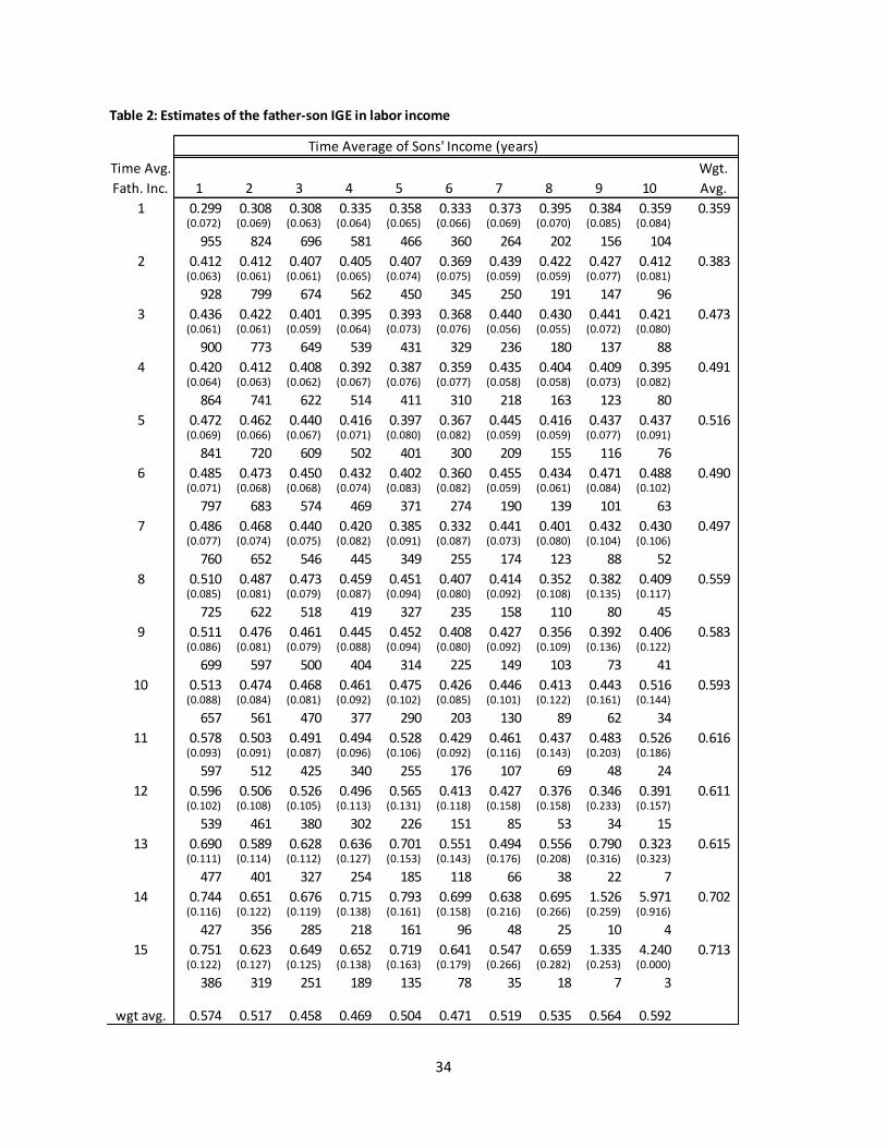
Table 2 shows a set of IGE estimates that only use the labor income of fathers and sons.

Appendix Table 2 presents similar estimates that also include the SEO samples. On the whole,

the estimates in Table 2 are fairly similar to those in Table 1 as is shown in Figure 3 which plots

the weighted average across the columns. For example, when using a 12-year average of fathers

income, the IGE when using labor income is 0.610 and when using family income the estimate is

0.612.

23

These estimates are broadly similar and slightly higher than those found by Mazumder

(2005a) who used the labor market earnings of fathers and sons from social security earnings

data. Mazumder (2005a) relied on several data imputation approaches to deal with issues related

to social security coverage and topcoding. However, with the PSID, none of these kinds of

imputations are necessary. These findings along with similar results in Mazumder (2005b) and

Mazumder and Acosta (2014) which also do not require imputations, suggest that the results of

Mazumder (2005a) are likely not due to the use of imputations as argued by Chetty et al (2014)

but instead are due to the longer time averages available in the SSA data and the PSID.

Sensitivity Checks in Chetty et al (2014)

Chetty et al (2014) argue that their national estimates of the IGE are unaffected by the

age at which children’s income is measured. They also argue that their estimates are unaffected

by the length of the time average used to measure parent income. They perform sensitivity

checks to demonstrate this empirically. In this section I describe why those sensitivity checks

are flawed and show how one can demonstrate this using the PSID. First, with respect to the

sensitivity of the IGE to the age at which child income is measured, Chetty et al (2014) claim

that while there is some lifecycle bias early in the career that this stabilizes once children have

reached the age of around 30. They conduct an empirical exercise that is shown in their

Appendix Figure IIA. They implement this sensitivity check by using an additional tax dataset

that includes much smaller intergenerational samples from the Statistics of Income (SOI). With

the SOI data they can examine the IGE between parents and children for earlier birth cohorts that

go back to 1971. They continue to use family income in 2011 and 2012 for children and the

period 1996 to 2000 for the parents. This implies that when they examine the 1971 cohort to

measure the IGE for 41 year olds they are actually using parent income that is measured when

24

the child was between the ages of 25 to 29 and unlikely to be living at home. Importantly, this

also implies that they are using the income of fathers when they are likely to be especially old.

For example, the income of a father who was 28 when his child was born in 1971 would be 53 to

57 years old when his income was measured in 1996 to 2000. Although Chetty et al do not

highlight these points, they have important implications. Using parent income at such late ages

when transitory fluctuations are a substantial part of earnings variation can lead to substantial

attenuation bias that could offset the reduction in lifecycle bias from measuring child income at

age 40 (Mazumder 2005a). Overall it could make it appear as though there is no lifecycle bias

when in fact it may actually be substantial.

With a long-running panel dataset like the PSID one can replicate this type of erroneous

sensitivity check but then also show the results differ if one allows the age at which children’s

income is measured to rise while simultaneously keeping the age at which father’s income is

measured, constant. To implement this exercise, I first replicate the findings in Chetty by

gradually increasing the age at which sons’ income is measured from 22 to 41 but

simultaneously increase the age range at which the five year average of father’s income is

measured to match the analogous age range implied by the tax data.15

In addition, one can also

fix this problem by using a 5 year time average that is always centered around the age of 40

while simultaneously raising the age of sons income from 22 to 41.

Figure 4 shows the results of this exercise. The red line replicates the basic pattern of

Chetty et al. Lifecycle bias appears to level off around the age of 30 and may even appear to

decline slightly in the late 30s. The green line demonstrates that this sensitivity check is flawed.

15

To fix ideas, for those sons who are aged 32, one would use the income of fathers when the child is between the ages of 15 and 19 as in Chetty et al. For those who are 33 one would use the income of fathers when the child is between 16 and 20 and so on.

25

While both lines track each other reasonably well before the age of 30, they start to diverge after

the age of 32. This is precisely around the time when the red line utilizes data on fathers when

the child is no longer in the home and when the fathers are entering their 50s and when their

income becomes noisy. With the green line, however, we continue to use centered time averages

of fathers around the age of 40 to eliminate this downward bias. The bottom line is that there is

in fact substantial lifecycle bias that cannot be uncovered by the sensitivity checks in the current

version of the tax data because of inherent data limitations.

There is also another pertinent sensitivity analysis around lengthening the time average of

parent income that Chetty et al present in their Figure 3B, Chetty et al do this by adding

additional years beyond the 1996-2000 time frame and show that their rank-rank slope estimates

do not increase, though they never show the results of this exercise for the IGE.16

The key

problem with this approach is that once again they must necessarily increase the attenuation bias

from using later ages in the lifecycle of parents as they extend the length of the time averages.

This can again have an offsetting effect due to attenuation bias. For example, the mean age of

fathers in their sample in 2003 exceeds 50 so once they start lengthening time averages to

include data in 2003 and beyond, they are actually including income observations with lots of

noise. And once again, when they extend the time averages in this manner they are actually

utilizing many years of income when they child is likely no longer living at home. With the

PSID, one can avoid this pitfall. Specifically, one can increase the length of the time average

while still holding constant the mean age of fathers by using centered time averages.

As before, I first use the PSID to replicate the results of the sensitivity check in Chetty at

al. and then show that time averaging does in fact reduce the attenuation bias once one removes

16

See Chetty et al (2014, Figure 3B).

26

the mechanical effect of increasing parent age.17

The results are shown in Figure 5. First, I am

able to replicate the spirit of the finding in Chetty et al’s Figure 3B. The red line shows that as I

extend the time average of fathers’ income by using years when the fathers are getting older, I

find that the time averages appear to have no effect on increasing estimates of the IGE. The IGE

stays flat at first and then actually starts to decline when the averages get very large. However,

when I use a centered time average of fathers’ income around the age of 40, a lengthening of the

time average generally leads to greater IGE estimates suggesting that larger time averages of

parent income do tend to reduce attenuation bias.

Rank-Rank Slope Estimates

In this section, I present an analogous set of results for the rank-rank slope. I begin by

showing the rank-rank slope estimate when using the main measure of family income that is

most similar to what is measured in the tax data and what was used to generate Table 1. The

results are shown in Table 3. With the rank-rank slope some new patterns emerge. First, it

appears that increasing the length of the time averages centered around the age of 40 for sons

does appear to increase the slope estimates. For example, looking over the first 10 rows, it

appears that in nearly every case that the slope estimates are higher when sons’ income is

averaged over 8, 9 or 10 years than just 1 or 2 years. This was not the case with the IGE. In

Table 1 it was typically the reverse pattern. It is not obvious why this is the case but perhaps

there is some aspect of lifecycle bias that is more pronounced when using ranks than when using

the IGE. This may be a fruitful issue for future research to investigate.

17

Specifically, use just a 2 year average of sons’ income over the ages of 29 to 32 and then start with a single year of fathers’ income that is measured when the son is 15 and then gradually add years of fathers’ income from subsequent years. For a five year average, this uses the income of fathers when the son is between the ages of 15 and 19. This mimics the 1981 birth cohort in Chetty et al whose parent income is measured in 1996 and 2000. A ten year average then utilizes the income of fathers when the son is between the ages of 15 and 24.

27

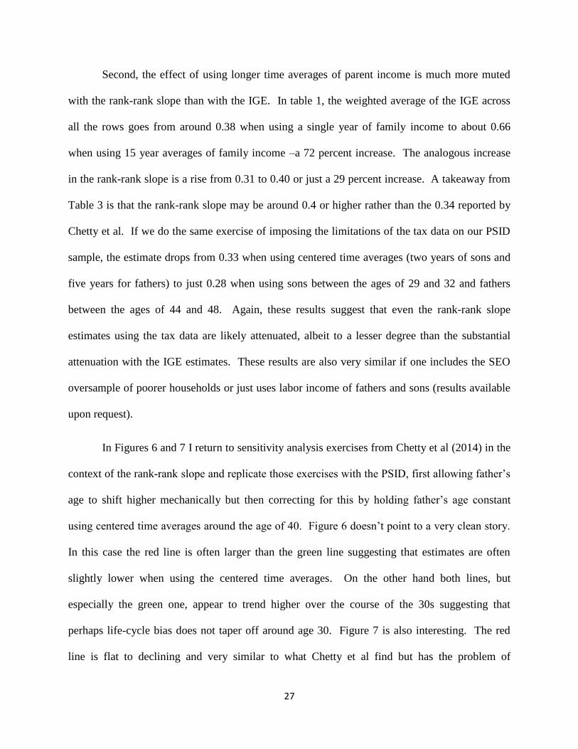
Second, the effect of using longer time averages of parent income is much more muted

with the rank-rank slope than with the IGE. In table 1, the weighted average of the IGE across

all the rows goes from around 0.38 when using a single year of family income to about 0.66

when using 15 year averages of family income –a 72 percent increase. The analogous increase

in the rank-rank slope is a rise from 0.31 to 0.40 or just a 29 percent increase. A takeaway from

Table 3 is that the rank-rank slope may be around 0.4 or higher rather than the 0.34 reported by

Chetty et al. If we do the same exercise of imposing the limitations of the tax data on our PSID

sample, the estimate drops from 0.33 when using centered time averages (two years of sons and

five years for fathers) to just 0.28 when using sons between the ages of 29 and 32 and fathers

between the ages of 44 and 48. Again, these results suggest that even the rank-rank slope

estimates using the tax data are likely attenuated, albeit to a lesser degree than the substantial

attenuation with the IGE estimates. These results are also very similar if one includes the SEO

oversample of poorer households or just uses labor income of fathers and sons (results available

upon request).

In Figures 6 and 7 I return to sensitivity analysis exercises from Chetty et al (2014) in the

context of the rank-rank slope and replicate those exercises with the PSID, first allowing father’s

age to shift higher mechanically but then correcting for this by holding father’s age constant

using centered time averages around the age of 40. Figure 6 doesn’t point to a very clean story.

In this case the red line is often larger than the green line suggesting that estimates are often

slightly lower when using the centered time averages. On the other hand both lines, but

especially the green one, appear to trend higher over the course of the 30s suggesting that

perhaps life-cycle bias does not taper off around age 30. Figure 7 is also interesting. The red

line is flat to declining and very similar to what Chetty et al find but has the problem of

28

conflating two different biases. The green line, which fixes the mechanical increase in fathers

age when taking longer time averages does show evidence of larger estimates but only when the

time averages are very long. The more muddled view from Figures 6 and 7 serve to reinforce the

more direct evidence from Table 3 and the results when imposing the tax data limitations.

Namely, estimates of the rank-rank slope are also likely biased down due the limitations of the

tax data but to a much lesser extent than the IGE.

VI. Conclusion

The literature on intergenerational mobility over the past few decades has shown how

attenuation bias and lifecycle bias can substantially affect estimates of the intergenerational

elasticity (IGE). Most previous estimates of the IGE in family income in the U.S. are around 0.5.

Using very large samples of tax records that are digitized going back only to 1996, Chetty et al

(2014) estimate that the IGE is actually much lower at 0.344. Further they make strong claims

that these estimates are not subject to attenuation bias or lifecycle bias. If accurate, this finding

is important because the IGE is an important gauge concerning the extent to which gaps between

families in America will dissipate over time and so it is important to understand whether the

evidence of greater mobility from the tax data is accurate or spurious.

I shed some light on this by describing the fundamental data limitations of the currently

available tax data. The key point is that the panel length is currently too short to do a good job

overcoming the issues concerning attenuation bias and lifecycle bias. I show that a long-lived

survey panel such as the PSID that may only have a few thousand families is actually more

useful for estimating the national IGE than having millions of tax records if the data are limited

in their ability to cover long stretches of the life course. Using longer and centered time averages

around the age of 40 I show that the IGE in family income is close to 0.7. I also show that when

29

I impose the same limitations as the tax data, that I obtain similar IGE estimates of around 0.3.

Further I demonstrate that the sensitivity checks used by Chetty et al to address concerns about

1) the age at which sons’ income is measured, and 2) the length of time averages of parent

income, are flawed. Correcting for the fact that their sensitivity checks are confounded by the

rising age at which parent income is measured, I show that the lifecycle bias and attenuation bias

almost surely exists in the tax data when estimating the IGE.

On the other hand, the results with the PSID with respect to the rank-rank slope suggest

that these biases are much smaller and that the rank-rank slope is relatively more robust (though

not entirely immune) from these measurement concerns. It is important, however, to remember

that the IGE is conceptually different from the rank-rank slope and may continue to be of

substantial value to researchers and policy-makers especially in an era of rising inequality when

gaps in society may be expanding. In that context focusing only on positional mobility because

measurement is easier, may not be appropriate.

Finally, it is important to make clear that Chetty et al (2014) makes a notable contribution

to the literature by demonstrating that there may be large geographic differences in

intergenerational mobility across the U.S. It is likely that these large geographic differences will

remain even after correcting for the biases in the tax data. Nevertheless, it may be useful for

future research to more directly examine this issue and verify that he central findings in their

paper are robust these biases.

30

References

Abowd, John and Martha Stinson. 2013. “Estimating Measurement Error in Annual Job

Earnings: A Comparison of Survey and Administrative Data” Review of Economics and

Statistics, 95(5):1451-1467.

Barro, Robert, and Xavier Sala-i-Martin. 1992. ‘‘Convergence.’’ Journal of Political Economy

100(2):223–51.

Bhattacharya, Debopam and Bhashkar Mazumder. 2011. “A nonparametric analysis of black–

white differences in intergenerational income mobility in the United States.” Quantitative

Economics, 2 (3): 335–379.

Black, Sandra E. and Paul J. Devereux. 2011. “Recent Developments in Intergenerational

Mobility.” in O. Ashenfelter and D. Card, eds., Handbook of Labor Economics, Vol. 4, Elsevier,

chapter 16, pp. 1487–1541.

Böhlmark, A. and Lindquist, M. (2006) ‘Life-Cycle Variations in the Association between

Current and Lifetime Income: Replication and Extension for Sweden’, Journal of Labor

Economics, 24(4), 879–896.

Bratberg, Espen, Jonathan Davis, Martin Nybom, Daniel Schnitzlein, and Kjell Vaage. 2015. “A

Comparison of Intergenerational Mobility Curves in Germany, Norway, Sweden and the U.S,”

working paper, University of Bergen.

Bratsberg, Bernt, Knut Røed, Oddbjørn Raaum, Robin Naylor, Markus Ja¨ntti, Tor Eriksson and

Eva O¨sterbacka 2007. “Nonlinearities in Intergenerational Earnings Mobility: Consequences

for Cross-Country Comparisons” Economic Journal 117(519):C72-C92

Chetty, Raj, Nathaniel Hendren, Patrick Kline, and Emmanuel Saez. 2014. “Where is the land of

Opportunity? The Geography of Intergenerational Mobility in the United States”. Quarterly

Journal of Economics, 129(4): 1553-1623.

Corak, Miles, Matthew Lindquist and Bhashkar Mazumder, 2014. “A Comparison of Upward

Intergenerational Mobility in Canada, Sweden and the United States” Labour Economics, 2014,

30: 185-200

Dahl, Molly and Thomas DeLeire. 2008. “The Association between Children’s Earnings and

Fathers’ Lifetime Earnings: Estimates Using Administrative Data.” Institute for Research on

Poverty, University of Wisconsin-Madison.

Grawe, N. D. (2006) ‘Lifecycle Bias in Estimates of Intergenerational Earnings Persistence’,

Labour Economics, 13(5), 551–570.

Hertz, Tom, 2005, “Rags, riches, and race: The intergenerational economic mobility of black and

white families in the United States,” in Unequal Chances: Family Background and Economic

31

Success, Samuel Bowles, Herbert Gintis, and Melissa Osborne Groves (eds.), Princeton, NJ:

Princeton University Press.

Hertz, Tom, 2006. “Understanding Mobility in America” Center for American Progress.

Hoyakem et al. (2012)

Hoyakem et al. (2015)

J¨antti, Markus, Bernt Bratsberg, Knut Røed, Oddbjørn Raaum, Robin Naylor, Eva ¨Osterbacka,

Anders Bj¨orklund, and Tor Eriksson. 2006. “American Exceptionalism in a New Light: A

Comparison of Intergenerational Earnings Mobility in the Nordic Countries, the United Kingdom

and the United States.” IZA Discussion Paper 1938, Institute for the Study of Labor (IZA).

Jenkins, S. (1987) ‘Snapshots versus Movies: ‘Lifecycle biases’ and the Estimation of

Intergenerational Earnings Inheritance’, European Economic Review, 31(5), 1149-1158.

Lee, Chul-In and Gary Solon. 2009. “Trends in Intergenerational Income Mobility.” The Review

of Economics and Statistics, 91 (4): 766–772.

Mazumder, Bhashkar. 2005a. “Fortunate Sons: New Estimates of Intergenerational Mobility in

the United States Using Social Security Earnings Data.” The Review of Economics and Statistics,

87 (2): 235–255.

Mazumder, Bhashkar. 2005b. “The Apple Falls Even Farther From the Tree Than We Thought:

New and Revised Estimates of the Intergenerational Inheritance of Earnings", Intergenerational

Inequality, Bowles, S., Gintis, H. and Osborne-Groves M. eds., Russell Sage Foundation,

Princeton.

Mazumder, Bhashkar. 2014. “Black-white differences in intergenerational economic mobility in

the United States.” Economic Perspectives, 38(1).

Mazumder, Bhashkar and Miguel Acosta. 2014. “Using Occupation to Measure

Intergenerational Mobility” with Miguel Acosta. The ANNALS of the American Academy of

Political and Social Science, 2015, 657: 174-193

Mulligan, Casey B., Parental Priorities and Economic Inequality (Chicago: University of

Chicago Press, 1997).

Nilsen, Oivind Anti, Kjell Vaage, Aarild Aavik, and Karl Jacobsen. 2012. “Intergenerational

Earnings Mobility Revisited: Estimates Based on Lifetime Earnings” Scandinavian Journal of

Economics, 114(1): 1-23.

32

Nybom, Martin amd Jan Stuhler. 2015. “Biases in Standard Measures of Intergenerational

Dependence.”

Solon, Gary. 1992. “Intergenerational Income Mobility in the United States.” American

Economic Review, 82 (3): 393–408.

Solon, Gary. 1999. “Intergenerational Mobility in the Labor Market.” in O. Ashenfelter and

D. Card, eds., Handbook of Labor Economics, Vol. 3, Elsevier, pp. 1761–1800.

33

Table 1: Estimates of the father-son IGE in family income

Time Avg. Wgt.

Fath. Inc. 1 2 3 4 5 6 7 8 9 10 Avg.

1 0.414 0.372 0.405 0.375 0.397 0.361 0.317 0.315 0.354 0.415 0.381(0.075) (0.067) (0.069) (0.068) (0.064) (0.070) (0.063) (0.068) (0.080) (0.091)

1358 1184 1050 932 786 595 440 351 267 183

2 0.439 0.420 0.434 0.402 0.429 0.443 0.391 0.379 0.419 0.453 0.423(0.066) (0.059) (0.062) (0.062) (0.068) (0.088) (0.067) (0.069) (0.082) (0.089)

1317 1145 1015 901 758 572 419 331 251 170

3 0.478 0.445 0.450 0.414 0.440 0.440 0.401 0.380 0.416 0.449 0.441(0.067) (0.060) (0.064) (0.064) (0.071) (0.088) (0.062) (0.066) (0.078) (0.088)

1268 1099 970 862 719 537 389 306 230 154

4 0.478 0.455 0.467 0.435 0.453 0.463 0.419 0.388 0.431 0.422 0.453(0.068) (0.061) (0.069) (0.069) (0.079) (0.105) (0.063) (0.067) (0.085) (0.091)

1216 1051 926 819 678 497 354 273 203 133

5 0.530 0.493 0.500 0.468 0.479 0.477 0.428 0.398 0.441 0.454 0.485(0.071) (0.065) (0.075) (0.076) (0.088) (0.113) (0.065) (0.069) (0.090) (0.098)

1175 1015 892 788 649 471 332 255 188 123

6 0.517 0.482 0.492 0.458 0.473 0.476 0.420 0.389 0.434 0.452 0.477(0.071) (0.066) (0.077) (0.078) (0.091) (0.120) (0.064) (0.067) (0.091) (0.092)

1120 966 843 741 606 431 299 228 165 105

7 0.529 0.485 0.492 0.459 0.464 0.462 0.379 0.369 0.399 0.402 0.474(0.077) (0.073) (0.086) (0.089) (0.105) (0.144) (0.065) (0.078) (0.109) (0.104)

1063 915 795 696 564 396 271 202 143 87

8 0.552 0.518 0.546 0.521 0.545 0.595 0.368 0.345 0.430 0.468 0.523(0.086) (0.082) (0.091) (0.096) (0.110) (0.166) (0.092) (0.114) (0.166) (0.156)

1005 863 747 648 520 354 232 168 114 67

9 0.573 0.537 0.558 0.536 0.560 0.629 0.435 0.391 0.494 0.624 0.548(0.090) (0.087) (0.096) (0.101) (0.115) (0.179) (0.090) (0.117) (0.183) (0.159)

956 818 710 614 488 326 208 147 97 54

10 0.580 0.529 0.545 0.521 0.550 0.633 0.421 0.388 0.502 0.698 0.544(0.095) (0.092) (0.101) (0.106) (0.124) (0.197) (0.092) (0.124) (0.201) (0.192)

895 766 660 569 449 298 185 129 83 45

11 0.630 0.567 0.590 0.576 0.602 0.691 0.460 0.380 0.461 0.650 0.588(0.099) (0.099) (0.107) (0.113) (0.134) (0.220) (0.093) (0.140) (0.234) (0.245)

818 696 595 510 399 255 149 98 59 31

12 0.648 0.592 0.623 0.589 0.624 0.747 0.474 0.386 0.400 0.604 0.612(0.109) (0.108) (0.117) (0.123) (0.151) (0.258) (0.119) (0.164) (0.247) (0.271)

743 633 541 465 358 224 121 78 46 24

13 0.667 0.612 0.649 0.625 0.605 0.533 0.462 0.287 0.395 0.363 0.612(0.122) (0.107) (0.110) (0.113) (0.114) (0.117) (0.155) (0.215) (0.301) (0.164)

656 554 470 399 307 184 96 57 31 13

14 0.714 0.692 0.714 0.681 0.659 0.629 0.511 0.457 0.986 0.761 0.685(0.129) (0.104) (0.116) (0.120) (0.122) (0.115) (0.182) (0.311) (0.411) (0.368)

590 495 415 349 263 146 70 36 15 7

15 0.680 0.664 0.662 0.616 0.651 0.597 0.532 0.576 1.527 0.954 0.656(0.134) (0.099) (0.109) (0.108) (0.123) (0.129) (0.216) (0.393) (0.258) (0.700)

533 448 374 309 228 120 54 24 11 6

wgt avg. 0.539 0.501 0.517 0.485 0.501 0.510 0.405 0.374 0.432 0.469

Time Average of Sons' Income (years)

34

Table 2: Estimates of the father-son IGE in labor income

Time Avg. Wgt.

Fath. Inc. 1 2 3 4 5 6 7 8 9 10 Avg.

1 0.299 0.308 0.308 0.335 0.358 0.333 0.373 0.395 0.384 0.359 0.359(0.072) (0.069) (0.063) (0.064) (0.065) (0.066) (0.069) (0.070) (0.085) (0.084)

955 824 696 581 466 360 264 202 156 104

2 0.412 0.412 0.407 0.405 0.407 0.369 0.439 0.422 0.427 0.412 0.383(0.063) (0.061) (0.061) (0.065) (0.074) (0.075) (0.059) (0.059) (0.077) (0.081)

928 799 674 562 450 345 250 191 147 96

3 0.436 0.422 0.401 0.395 0.393 0.368 0.440 0.430 0.441 0.421 0.473(0.061) (0.061) (0.059) (0.064) (0.073) (0.076) (0.056) (0.055) (0.072) (0.080)

900 773 649 539 431 329 236 180 137 88

4 0.420 0.412 0.408 0.392 0.387 0.359 0.435 0.404 0.409 0.395 0.491(0.064) (0.063) (0.062) (0.067) (0.076) (0.077) (0.058) (0.058) (0.073) (0.082)

864 741 622 514 411 310 218 163 123 80

5 0.472 0.462 0.440 0.416 0.397 0.367 0.445 0.416 0.437 0.437 0.516(0.069) (0.066) (0.067) (0.071) (0.080) (0.082) (0.059) (0.059) (0.077) (0.091)

841 720 609 502 401 300 209 155 116 76

6 0.485 0.473 0.450 0.432 0.402 0.360 0.455 0.434 0.471 0.488 0.490(0.071) (0.068) (0.068) (0.074) (0.083) (0.082) (0.059) (0.061) (0.084) (0.102)

797 683 574 469 371 274 190 139 101 63

7 0.486 0.468 0.440 0.420 0.385 0.332 0.441 0.401 0.432 0.430 0.497(0.077) (0.074) (0.075) (0.082) (0.091) (0.087) (0.073) (0.080) (0.104) (0.106)

760 652 546 445 349 255 174 123 88 52

8 0.510 0.487 0.473 0.459 0.451 0.407 0.414 0.352 0.382 0.409 0.559(0.085) (0.081) (0.079) (0.087) (0.094) (0.080) (0.092) (0.108) (0.135) (0.117)

725 622 518 419 327 235 158 110 80 45

9 0.511 0.476 0.461 0.445 0.452 0.408 0.427 0.356 0.392 0.406 0.583(0.086) (0.081) (0.079) (0.088) (0.094) (0.080) (0.092) (0.109) (0.136) (0.122)

699 597 500 404 314 225 149 103 73 41

10 0.513 0.474 0.468 0.461 0.475 0.426 0.446 0.413 0.443 0.516 0.593(0.088) (0.084) (0.081) (0.092) (0.102) (0.085) (0.101) (0.122) (0.161) (0.144)

657 561 470 377 290 203 130 89 62 34

11 0.578 0.503 0.491 0.494 0.528 0.429 0.461 0.437 0.483 0.526 0.616(0.093) (0.091) (0.087) (0.096) (0.106) (0.092) (0.116) (0.143) (0.203) (0.186)

597 512 425 340 255 176 107 69 48 24

12 0.596 0.506 0.526 0.496 0.565 0.413 0.427 0.376 0.346 0.391 0.611(0.102) (0.108) (0.105) (0.113) (0.131) (0.118) (0.158) (0.158) (0.233) (0.157)

539 461 380 302 226 151 85 53 34 15

13 0.690 0.589 0.628 0.636 0.701 0.551 0.494 0.556 0.790 0.323 0.615(0.111) (0.114) (0.112) (0.127) (0.153) (0.143) (0.176) (0.208) (0.316) (0.323)

477 401 327 254 185 118 66 38 22 7

14 0.744 0.651 0.676 0.715 0.793 0.699 0.638 0.695 1.526 5.971 0.702(0.116) (0.122) (0.119) (0.138) (0.161) (0.158) (0.216) (0.266) (0.259) (0.916)

427 356 285 218 161 96 48 25 10 4

15 0.751 0.623 0.649 0.652 0.719 0.641 0.547 0.659 1.335 4.240 0.713(0.122) (0.127) (0.125) (0.138) (0.163) (0.179) (0.266) (0.282) (0.253) (0.000)

386 319 251 189 135 78 35 18 7 3

wgt avg. 0.574 0.517 0.458 0.469 0.504 0.471 0.519 0.535 0.564 0.592

Time Average of Sons' Income (years)

35

Table 3: Estimates of the father-son rank-rank slope in family income

Time Avg. Wgt.

Fath. Inc. 1 2 3 4 5 6 7 8 9 10 Avg.

1 0.282 0.304 0.326 0.309 0.333 0.322 0.295 0.290 0.307 0.423 0.310(0.032) (0.036) (0.039) (0.040) (0.043) (0.050) (0.059) (0.065) (0.071) (0.080)

1358 1184 1050 932 786 595 440 351 267 183

2 0.290 0.312 0.341 0.329 0.362 0.376 0.352 0.339 0.356 0.448 0.334(0.032) (0.035) (0.038) (0.040) (0.043) (0.050) (0.059) (0.065) (0.073) (0.083)

1317 1145 1015 901 758 572 419 331 251 170

3 0.296 0.317 0.341 0.328 0.362 0.379 0.373 0.352 0.375 0.451 0.338(0.032) (0.035) (0.039) (0.041) (0.043) (0.049) (0.055) (0.065) (0.072) (0.086)

1268 1099 970 862 719 537 389 306 230 154

4 0.296 0.320 0.347 0.333 0.366 0.391 0.396 0.363 0.389 0.435 0.343(0.032) (0.036) (0.039) (0.041) (0.044) (0.050) (0.055) (0.067) (0.078) (0.096)

1216 1051 926 819 678 497 354 273 203 133

5 0.309 0.333 0.362 0.348 0.378 0.399 0.413 0.374 0.402 0.482 0.357(0.032) (0.036) (0.040) (0.042) (0.045) (0.052) (0.058) (0.069) (0.083) (0.097)

1175 1015 892 788 649 471 332 255 188 123

6 0.299 0.319 0.348 0.333 0.362 0.385 0.404 0.365 0.399 0.504 0.344(0.034) (0.037) (0.042) (0.044) (0.047) (0.054) (0.063) (0.072) (0.088) (0.095)

1120 966 843 741 606 431 299 228 165 105

7 0.283 0.302 0.328 0.311 0.336 0.350 0.370 0.316 0.339 0.436 0.318(0.035) (0.039) (0.044) (0.046) (0.049) (0.057) (0.067) (0.076) (0.095) (0.104)

1063 915 795 696 564 396 271 202 143 87

8 0.282 0.303 0.336 0.321 0.348 0.362 0.332 0.279 0.280 0.396 0.317(0.037) (0.042) (0.046) (0.049) (0.052) (0.062) (0.075) (0.088) (0.112) (0.123)

1005 863 747 648 520 354 232 168 114 67

9 0.292 0.309 0.342 0.333 0.365 0.394 0.403 0.327 0.318 0.493 0.334(0.038) (0.043) (0.048) (0.050) (0.053) (0.062) (0.071) (0.091) (0.125) (0.113)

956 818 710 614 488 326 208 147 97 54

10 0.287 0.304 0.330 0.319 0.352 0.379 0.397 0.330 0.314 0.539 0.325(0.039) (0.044) (0.049) (0.051) (0.054) (0.064) (0.074) (0.098) (0.138) (0.134)

895 766 660 569 449 298 185 129 83 45

11 0.299 0.315 0.345 0.338 0.364 0.394 0.413 0.315 0.267 0.518 0.336(0.040) (0.046) (0.051) (0.054) (0.057) (0.069) (0.080) (0.112) (0.162) (0.169)

818 696 595 510 399 255 149 98 59 31

12 0.310 0.326 0.354 0.336 0.363 0.386 0.390 0.303 0.236 0.587 0.339(0.042) (0.049) (0.054) (0.057) (0.062) (0.077) (0.093) (0.125) (0.179) (0.196)

743 633 541 465 358 224 121 78 46 24

13 0.335 0.355 0.392 0.384 0.385 0.357 0.311 0.133 0.076 0.264 0.354(0.046) (0.051) (0.055) (0.057) (0.065) (0.088) (0.118) (0.162) (0.232) (0.295)

656 554 470 399 307 184 96 57 31 13

14 0.356 0.391 0.433 0.428 0.432 0.445 0.400 0.322 0.446 0.618 0.403(0.048) (0.050) (0.055) (0.057) (0.066) (0.088) (0.127) (0.191) (0.285) (0.244)

590 495 415 349 263 146 70 36 15 7

15 0.350 0.382 0.428 0.426 0.447 0.436 0.418 0.399 0.635 0.423 0.401(0.050) (0.051) (0.057) (0.057) (0.068) (0.095) (0.137) (0.242) (0.231) (0.382)

533 448 374 309 228 120 54 24 11 6

wgt avg. 0.300 0.321 0.350 0.337 0.364 0.377 0.371 0.329 0.346 0.457

Time Average of Sons' Income (years)

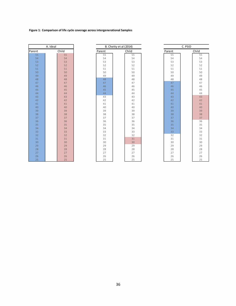
36

Figure 1: Comparison of life cycle coverage across intergenerational Samples

Parent Child Parent Child Parent Child55 55 55 55 55 5554 54 54 54 54 5453 53 53 53 53 5352 52 52 52 52 5251 51 51 51 51 5150 50 50 50 50 5049 49 49 49 49 4948 48 48 48 48 4847 47 47 47 47 4746 46 46 46 46 4645 45 45 45 45 4544 44 44 44 44 4443 43 43 43 43 4342 42 42 42 42 4241 41 41 41 41 4140 40 40 40 40 4039 39 39 39 39 3938 38 38 38 38 3837 37 37 37 37 3736 36 36 36 36 3635 35 35 35 35 3534 34 34 34 34 3433 33 33 33 33 3332 32 32 32 32 3231 31 31 31 31 3130 30 30 30 30 3029 29 29 29 29 2928 28 28 28 28 2827 27 27 27 27 2726 26 26 26 26 2625 25 25 25 25 25

A. Ideal C. PSIDB. Chetty et al (2014)

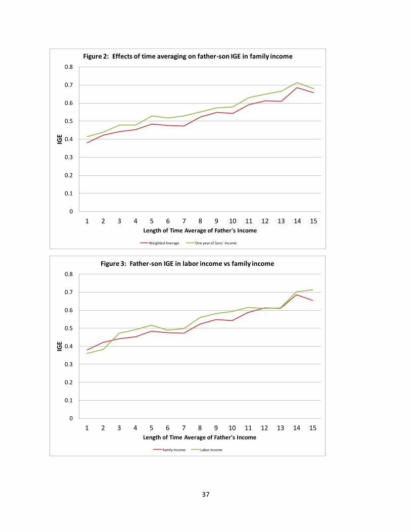
37

0

0.1

0.2

0.3

0.4

0.5

0.6

0.7

0.8

1 2 3 4 5 6 7 8 9 10 11 12 13 14 15

IGE

Length of Time Average of Father's Income

Figure 2: Effects of time averaging on father-son IGE in family income

Weighted Average One year of Sons' Income

0

0.1

0.2

0.3

0.4

0.5

0.6

0.7

0.8

1 2 3 4 5 6 7 8 9 10 11 12 13 14 15

IGE

Length of Time Average of Father's Income

Figure 3: Father-son IGE in labor income vs family income

Family Income Labor Income

38

0

0.1

0.2

0.3

0.4

0.5

0.6

0.7

0.8

0.9

1

22 23 24 25 26 27 28 29 30 31 32 33 34 35 36 37 38 39 40 41

IGE

Age of Son

Figure 4: Re-examining the Sensitivity of the IGE to Son's Age

Replicating the Chetty et al Approach Fixing the Sensitivity Check

0

0.1

0.2

0.3

0.4

0.5

0.6

0.7

1 2 3 4 5 6 7 8 9 10 11 12 13 14 15 16 17

IGE

Length of Time Average of Father's Income

Figure 5: Re-examining the Sensitivity of the IGE to longer time averages of parent income

Replicating the Chetty et al Approach Fixing the Sensitivity Check

39

0

0.05

0.1

0.15

0.2

0.25

0.3

0.35

0.4

0.45

22 23 24 25 26 27 28 29 30 31 32 33 34 35 36 37 38 39 40 41

IGE

Age of Son

Figure 6: Re-examining the Sensitivity of the Rank-rank Slope to Son's Age

Replicating the Chetty et al Approach Fixing the Sensitivity Check

0

0.05

0.1

0.15

0.2

0.25

0.3

0.35

0.4

0.45

1 2 3 4 5 6 7 8 9 10 11 12 13 14 15 16 17

IGE

Length of Time Average of Father's Income

Figure 7: Re-examining the Sensitivity of the rank-rank Slope to longer time averages of parent income

Replicating the Chetty et al Approach Fixing the Sensitivity Check

40

Appendix Table 1: Estimates of the father-son IGE in family income using SEO subsample

Time Avg. Wgt.

Fath. Inc. 1 2 3 4 5 6 7 8 9 10 Avg.

1 0.451 0.403 0.434 0.414 0.426 0.393 0.357 0.363 0.383 0.401 0.415(0.054) (0.048) (0.049) (0.051) (0.047) (0.050) (0.047) (0.054) (0.066) (0.077)

2133 1842 1611 1400 1158 867 623 490 364 251

2 0.485 0.450 0.468 0.438 0.457 0.451 0.406 0.402 0.418 0.430 0.453(0.053) (0.045) (0.047) (0.049) (0.052) (0.061) (0.048) (0.053) (0.063) (0.069)

2062 1774 1550 1345 1109 828 590 460 340 234

3 0.526 0.476 0.491 0.457 0.476 0.473 0.439 0.428 0.446 0.461 0.480(0.056) (0.049) (0.054) (0.053) (0.059) (0.068) (0.051) (0.054) (0.065) (0.074)

1989 1706 1483 1287 1054 780 548 427 313 213

4 0.531 0.487 0.508 0.476 0.487 0.493 0.449 0.435 0.464 0.443 0.492(0.058) (0.051) (0.058) (0.059) (0.066) (0.080) (0.052) (0.056) (0.072) (0.079)

1865 1594 1389 1200 975 709 491 379 278 186

5 0.586 0.526 0.544 0.510 0.514 0.508 0.457 0.446 0.482 0.483 0.527(0.062) (0.056) (0.066) (0.067) (0.076) (0.092) (0.058) (0.062) (0.082) (0.093)

1780 1519 1320 1137 917 661 452 346 253 167

6 0.575 0.515 0.535 0.499 0.506 0.503 0.437 0.425 0.476 0.481 0.518(0.063) (0.056) (0.068) (0.069) (0.079) (0.097) (0.057) (0.062) (0.086) (0.094)

1677 1429 1235 1057 848 597 398 300 215 137

7 0.593 0.528 0.548 0.514 0.516 0.513 0.420 0.418 0.446 0.428 0.528(0.067) (0.063) (0.076) (0.079) (0.093) (0.119) (0.060) (0.071) (0.099) (0.102)

1579 1343 1155 984 783 543 357 263 186 115

8 0.595 0.544 0.576 0.546 0.554 0.587 0.422 0.411 0.480 0.514 0.553(0.073) (0.069) (0.077) (0.081) (0.090) (0.125) (0.079) (0.097) (0.137) (0.136)

1490 1266 1087 918 724 490 313 225 154 95

9 0.616 0.560 0.588 0.560 0.571 0.622 0.479 0.461 0.546 0.660 0.577(0.077) (0.073) (0.081) (0.085) (0.094) (0.135) (0.077) (0.102) (0.153) (0.140)

1405 1190 1025 862 674 447 276 195 129 74

10 0.633 0.558 0.587 0.555 0.575 0.645 0.476 0.451 0.547 0.691 0.582(0.082) (0.079) (0.087) (0.092) (0.105) (0.157) (0.086) (0.109) (0.170) (0.155)

1321 1123 961 803 623 410 245 172 112 63

11 0.674 0.584 0.618 0.587 0.599 0.669 0.471 0.385 0.470 0.606 0.608(0.087) (0.086) (0.093) (0.099) (0.114) (0.179) (0.084) (0.119) (0.195) (0.183)

1182 1003 849 703 540 342 194 130 81 44

12 0.700 0.610 0.650 0.601 0.620 0.720 0.482 0.381 0.415 0.617 0.633(0.097) (0.095) (0.103) (0.110) (0.131) (0.214) (0.108) (0.143) (0.215) (0.226)

1068 903 764 632 478 297 158 103 63 34

13 0.714 0.619 0.656 0.621 0.598 0.526 0.454 0.291 0.392 0.389 0.625(0.111) (0.097) (0.099) (0.104) (0.104) (0.106) (0.144) (0.187) (0.251) (0.161)

942 794 667 546 414 248 126 78 45 21

14 0.769 0.698 0.721 0.678 0.651 0.616 0.507 0.436 0.909 0.859 0.700(0.118) (0.094) (0.106) (0.112) (0.112) (0.104) (0.170) (0.274) (0.354) (0.353)

831 694 581 471 350 193 88 48 21 8

15 0.752 0.675 0.677 0.626 0.653 0.598 0.546 0.569 1.318 1.094 0.682(0.123) (0.090) (0.099) (0.100) (0.112) (0.114) (0.200) (0.335) (0.334) (0.642)

745 624 521 419 304 163 70 34 16 7

wgt avg. 0.587 0.526 0.549 0.515 0.522 0.524 0.435 0.415 0.461 0.479

Time Average of Sons' Income (years)

41

0

0.1

0.2

0.3

0.4

0.5

0.6

0.7

0.8

0.9

1 2 3 4 5 6 7 8 9 10 11 12 13 14 15

IGE

Length of Time Average of Father's Income

Appendix Figure 1: Effects of time averaging on father-son IGE in family income including SEO sample

Weighted Average One year of Sons' Income