Embed Size (px)
Citation preview

ESTIMATION OF INTEGRATED SQUARED DENSITY DERIVATIVES
by
Brian Kent Aldershof
A dissertation submitted to the faculty of The University of North Carolina at Chapel Hill in
partial fulfillment of the requirements for the degree of Doctor of Philosophy in the Department
of Statistics.
Chapel Hill
1991
Advisor
Reader
UL~./~Reader
----'---+t----'---"'----
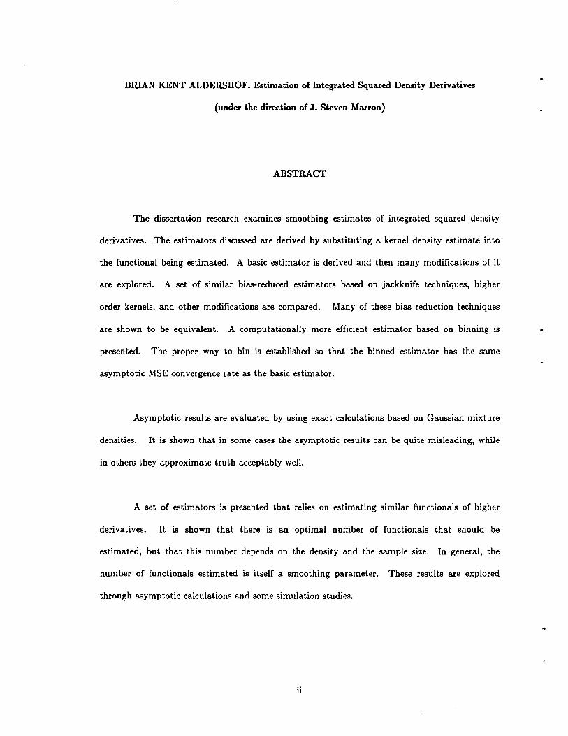
BRIAN KENT ALDERSHOF. Estimation of Integrated Squared Density Derivatives
(under the direction of J. Steven Marron)
ABSTRACT
The dissertation research examines smoothing estimates of integrated squared density
derivatives. The estimators discussed are derived by substituting a kernel density estimate into
the functional being estimated. A basic estimator is derived and then many modifications of it
are explored. A set of similar bias-reduced estimators based on jackknife techniques, higher
order kernels, and other modifications are compared. Many of these bias reduction techniques
are shown to be equivalent. A computationally more efficient estimator based on binning is
presented. The proper way to bin is established so that the binned estimator has the same
asymptotic MSE convergence rate as the basic estimator.
Asymptotic results are evaluated by using exact calculations based on Gaussian mixture
densities. It is shown that in some cases the asymptotic results can be quite misleading, while
in others they approximate truth acceptably well.
A set of estimators is presented that relies on estimating similar functionals of higher
derivatives. It is shown that there is an optimal number of functionals that should be
estimated, but that this number depends on the density and the sample size. In general, the
number of functionals estimated is itself a smoothing parameter. These results are explored
through asymptotic calculations and some simulation studies.
ii

ACKNOWLEDGEMENTS
I am very grateful for the encouragement, support, and guidance of my advisor Dr. J.
Steven Marron. His insights and intuition led to many of the results here. His patient
encouragement helped me through rough times. Thanks, Steve.
I am grateful to the people who supported me and my family throughout my years in
Graduate School. In particular, thanks to my mother who always helped out. Thanks also to
my in-laws for their support.
Most of all, I want to thank my wife and daughter. My family has always been loving
and supportive despite Graduate School poverty and uncertainty. Welcome to the world, Nick.
iii
TABLE OF CONTENTS
Page
LIST OF TABLES vi
LIST OF FIGURES vii
Chapter
I. Introduction and Literature Review
1. Introduction 1
2. Literature Review 3
II. Diagonal Terms
1. Introduction 13
2. Bias Reduction 14
3. Mean Squared Error Reduction 15
4. Computation 23
5. Stepped Estimators 24
III. Bias Reduction
1. Introduction 25
2. Notation 26
3. Higher Order Kernel Estimators 26
4. D - Estimators 27
5. Generalized Jackknife Estimators 28
6. Higher Order Generalized Jackknife Estimators 29
7. Relationships Among Bias Reduction Estimators 30
8. Theorems 32
9. Example 34
10. Proofs 38
IV. Computation
1. Introduction 48
2. Notation 49
3. The Histogram Binned Estimator : 50
4. Computation of 8m (h, n, K) 53
5. Generalized Bin Estimator 54
6. Proofs 57
iv
V. Asymptotics and Exact Calculations
1. Introduction 69
2. Comparison of Asymptotic and Exact Risks 69
3. Exact MSE Calculations 73
4. Examples 77
5. Proofs 80
VI. Estimability of 8m and m
1. Introduction 84
2. Asymptotic Calculations 84
3. Exact MSE Calculations 86
VII. The One - Step Estimator
1. Introduction 92
2. Assumptions and Notation 93
3. Results 94
4. Figures 100
5. Conclusions 101
6. Proofs 106
7. em(t) and calculating the skewness of 8m (h, n, K) 115
VIII. The K - Step Estimator
1. Introduction 118
2. Assumptions and Notation 120
3. Results 121
4. Simulations 125
5. Conclusions 127
6. Proofs 132
Appendix A viii
v
Table 2.1:
Table 2.2:
Table 6.1a:
Table 6.1b:
LIST OF TABLES
Exact Asymptotic Values of MSEj02 21
"Plug-in" Values of MSEj02 22
Values of N1/ 2(m) for m=O, , 5; Distns 1-8 89
Values of N1/ 2(m) for m=O, , 5; Distns 9-15 90
vi
Figure 3.1:
Figure 3.2a:
Figure 3.2b:
Figure 3.2c
Figure 5.1:
Figure 5.2:
Figure 6.1a:
Figure 6.1b:
Figure 7.1a:
Figure 7.1b:
Figure 7.2a:
Figure 7.2b:
Figure 7.3a:
Figure 7.3b:
Figure 7Aa:
Figure 7Ab:
Figure 8.1a:
Figure 8.1b:
Figure 8.2a:
Figure 8.2b:
Figure 8.3a:
Figure 8.3b:
Figure 804:
LIST OF FIGURES
Equivalences of Bias Reduction Techniques 31
D-estimator kernels 36
Jackknife kernels 36
Second-order kernel 37
MSE vs log(Bandwidth) (Distn #4; Sample Size = 1000) 79
MSE vs log(Bandwidth) (Distn #11; Sample Size = 1000) 79
Ntol(O) vs tolerance 91
Ntol(l) vs tolerance 91
MSE vs Bandwidth (Distn #2; Sample Size = 250) 103
MSE vs Bandwidth (Distn #2; Sample Size = 1000) 103
MSE vs log(Bandwidth) (Distn #2; Sample Size = 250) 104
MSE vs log(Bandwidth) (Distn #2; Sample Size = 1000) 104
MSE vs Bandwidth (Distn #2; Sample Size = 250) 105
MSE vs Bandwidth (Distn #2; Sample Size = 1000) 105
C2(T) vs T (Distn #1; Sample Size = 250) 117
C2(T) vs T (Distn #1; Sample Size = 1000) 117
Theta-hat densities (Distn #6; Squared 1st DerivativeSS=100; 100 Samples) 128
Theta-hat densities (Distn #6; Squared 1st DerivativeSS=100; 100 Samples) 128
Theta-hat densities (Distn #3; Squared 1st DerivativeSS=100; 100 Samples) : 129
Bandwidth densities (Distn #3; Squared 1st DerivativeSS=100; 100 Samples) 129
MSE vs Step (Distn #6; Sample Size = 100) 130
MSE vs Step (Distn #6; Sample Size = 500) 130
MSE vs Step (Distn #3; Sample Size = 100) 131
vii
Chapter I: Introduction and Literature Review
1. Introduction
This research discusses a class of estimators of the functional Om = J(im)Yfor fa
probability density function. The estimators discussed in this dissertation are of the form:
(1.1)
for some D which mayor may not be a function of the data. The goal of the research is to
discuss the behavior of these estimators in a variety of settings and to provide guidelines for
computing them.
Chapter II discusses possible choices of D given in (1.1). D can be chosen to reduce bias
simply by including the diagonal terms of the double sum thereby making Bnecessarily positive.
In many settings, this estimator performs better than a "leave-out-the-diagonals" version with
D = O. A possibly better estimator chosen to reduce MSE is also given although with reasonable
sample sizes this did not perform as well as hoped.
Chapter III discusses three strategies for reducing bias in B. The "leave-in-the-..
diagonals" estimator is some improvement over the "no-diagonals" estimator because it reduces
bias with some choice of bandwidth. More sophisticated strategies for reducing bias can improve
the estimator even more (at least with a sufficiently large sample size). The three strategies
explored are jackknifing, higher order kernels, and special choices of D (as in (1.1)). Some
equivalences between these techniques are given.
..
Chapter IV discusses computation of the estimators using a strategy called "binning".
Binning is used to reduce the number of computationally intensive kernel evaluations. An
optimal binning strategy is given in this chapter.
Chapter V discusses asymptotic calculations. Many of the guidelines presented in this
dissertation and in many areas of density estimation rely on asymptotic results. This chapter
provides some comparison of these results to exact results. A tool used to do this is exact
calculations based on Gaussian mixtures. Theorems required to do these calculations are
presented here.
Chapter VI provides some guidelines about the relative difficulty of estimating (Jm
compared to (Jm+k. Both asymptotic and exact calculations are used to show that it gets much
more difficult to estimate (Jm for greater m. It is also shown that the asymptotic calculations
become increasingly misleading in this context as m increases.
Chapter VII discusses a "one-step" estimator for choosing the bandwidth of Bm • The
estimator is based on estimating (Jm+l first and using this estimate to find an "optimal"
bandwidth for Bm . The results given here suggest that there may be some advantages to using
the one-step estimator in that it might be easier to choose a near-optimal bandwidth. The
penalty for using this estimator is that it has a greater minimum MSE than the standard
estimator.
Chapter VIII discusses a generalization of the one-step estimator called the "k-step"
estimator. In the "k-step" estimator all the functionals (Jm+!' .•., (Jm+k are estimated and used
to provide a bandwidth for Bm . It is shown there that with a finite sample size and a "plug-in"
bandwidth, MSE(Bm ) decreases for the first couple of steps and ultimately increases without
bound.
2
The remainder of this chapter is a literature review of previous research on the topic.
2. Literature Review.
The dissertation research concerns the study of the estimation of functionals of the form
0m(f) = JV(m)(x)Y dx. Although there are several ways of estimating functionals of this
type, only kernel-type estimators will be investigated here. A kernel estimator in(x) of J(x) is
defined as
where Kh(x) = 11h K(xlh) , K is bounded and symmetric with JK(u) = 1, hn is the
bandwidth, and n is the sample size. Estimators of 0m(f) that will be studied here will be based
on this type of kernel estimator although other possibilities are discussed below.
2.1) Estimating 0o(f) = Jf2(x) dx.
Estimating 0o(f) is an important problem in calculating the asymptotic relative
efficiencies (ARE) of non-parametric, rank-based statistics. For example, consider testing Ho:
G(x) = F(x) vs. HI: G(x) = F(x - 0) where ° > 0, F and G are unknown, and F has density f
and variance (1'2. The ARE of the Wilcoxon test to the t-test is 12(1"Oo(f)f (Hodges and
Lehmann, 1956). The same result holds in the more general analysis of variance problem for the
ARE of the Kruskal-Wallis test relative to the standard F-test. The problem of estimating 0o(f)
naturally arises from forming a data-based estimate of these ARE's.
0o(J) can also be used in computing the L2 distance between two densities. In this
setting, estimation of 0o(J) has arisen in pattern recognition (Patrick and Fischer, 1969), data
3
reduction (Fukunga and Mantock, 1984), and other areas (Pawlak, 1986).
A straight-forward estimator of ()o(J) is derived by squaring and integrating an estimate
of f. Bhattacharya and Roussas (1969) proposed ();(in) = Jin2(x) dx as an estimator of ();(f),
where in(x) is a kernel density estimator. Substitution of in(x) gives
where * denotes convolution. Ahmad (1976) proved that with suitably chosen bandwidths,
();(in) - ()o(J) with probability 1 and established a rate of convergence.
Another estimator of ()o(J) is motivated by noting that:
Jf2(x) dx = E(J(x)) = JJ(x) dF(x).
An estimator of ()o(J) proposed by Schuster (1974) is ()o(in)
the empirical distribution function. Substitution gives
Notice that ();(in) can always be expressed as ()o(in)' For kernel functions, ()o(in) uses Kh andn
();(in) uses Kh * Kh · A simple change of variables shows that K" * Kh = (K. K)h so then n .~ n n
class of estimators ();(in) is the class of ()o(in) restricted to densities which are convolutions. If
K is a Gaussian density, ()o(in) and ();(in) are identical except for different bandwidths. Since
they are the same estimators it seems that ()o(in) and ();(in) should be equally good estimators
of ()o(J). Indeed, Schuster (1974) showed that ()o(in) and ();(in) converge to ()o(J) at the same
rate. Ahmad (1976) proved that under some conditions (fewer than used by Schuster) ()o(in) is
4
strongly consistent and asymptotically normal.
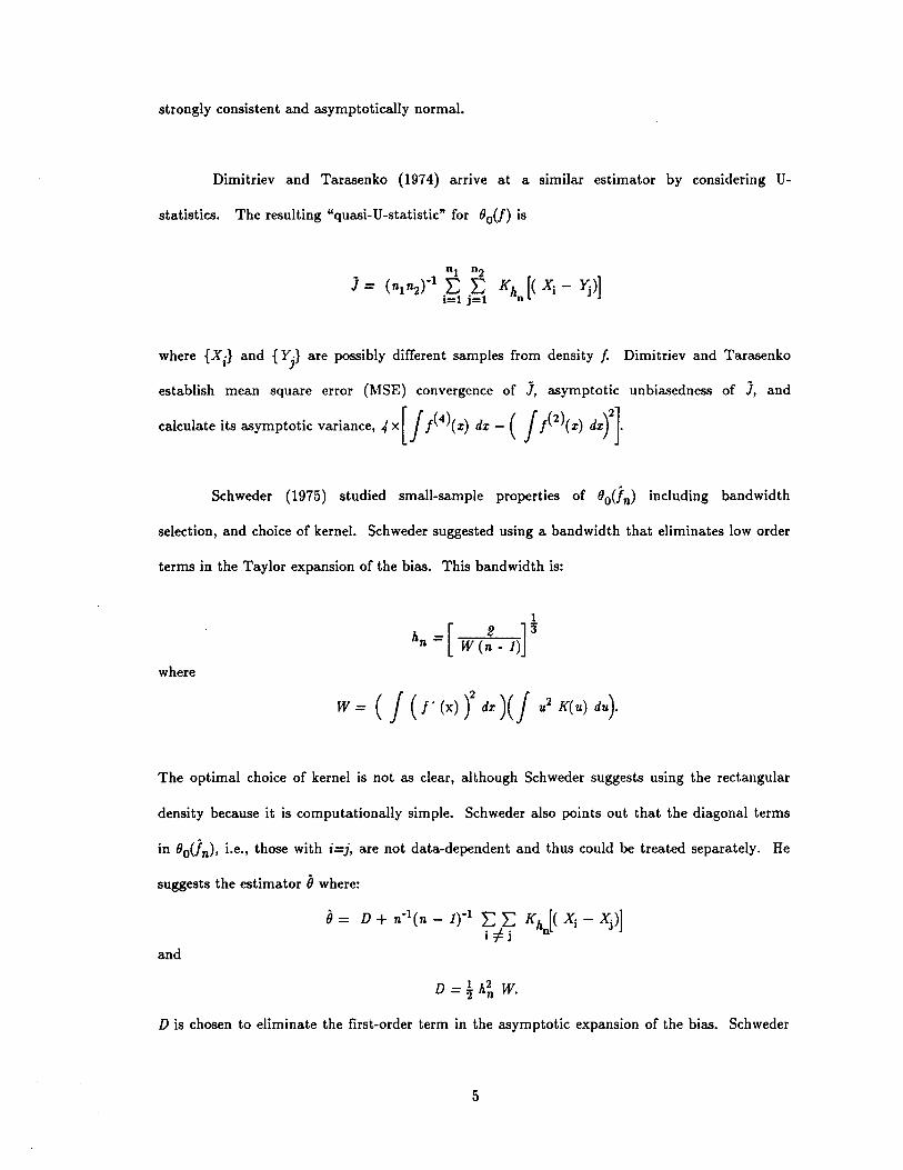
Dimitriev and Tarasenko (1974) arrive at a similar estimator by considering U-
statistics. The resulting "quasi-U-statistic" for (}o(f) is
where {Xi} and {Yj } are possibly different samples from density f. Dimitriev and Tarasenko
establish mean square error (MSE) convergence of i, asymptotic unbiasedness of i, and
calculate its asymptotic variance, 4x[/ /4)(x) dx - ( / /2)(x) dxt].
Schweder (1975) studied small-sample properties of (}o(in) including bandwidth
selection, and choice of kernel. Schweder suggested using a bandwidth that eliminates low order
terms in the Taylor expansion of the bias. This bandwidth is:
1
hn = [ W (: _ 1)]:3where
w = ( / (r (x) )2 dx )(/ u2 K(u) dU).
The optimal choice of kernel is not as clear, although Schweder suggests using the rectangular
density because it is computationally simple. Schweder also points out that the diagonal terms
in (}o(in), Le., those with i=j, are not data-dependent and thus could be treated separately. He
suggests the estimator iJ where:
and
D is chosen to eliminate the first-order term in the asymptotic expansion of the bias. Schweder
5
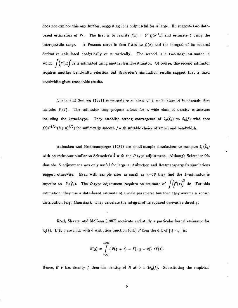
does not explore this any further, suggesting it is only useful for n large. He suggests two data-
based estimators of W. The first is to rewrite j{x) = 6-1/ 1(6-1x) and estimate 6 using the
interquartile range. A Pearson curve is then fitted to 11(x) and the integral of its squared
derivative calculated analytically or numerically. The second is a two-stage estimator in
which J(/'(x)y dx is estimated using another kernel-estimator. Of course, this second estimator
requires another bandwidth selection but Schweder's simulation results suggest that a fixed
bandwidth gives reasonable results.
Cheng and Sertling (1981) investigate estimation of a wider class of functionals that
includes °0(1). The estimator they propose allows for a wide class of density estimators
including the kernel-type. They establish strong convergence of (}o(in) to (}O(l) with rate
O(n-1/2 (log n)I/2) for sufficiently smooth Iwith suitable choice of kernel and bandwidth.
Aubuchon and Hettmansperger (1984) use small-sample simulations to compare (}o(in)
with an estimator similar to Schweder's iJ with the D-type adjustment. Although Schweder felt
that the D adjustment was only useful for large n, Aubuchon and Hettmansparger's simulations
suggest otherwise. Even with sample sizes as small as n=10 they find the D-estimator is
superior to 0o(fn). The D-type adjustment requires an estimate of J(/'(x)y dx. For this
estimation, they use a data-based estimate of a scale parameter but then they assume a known
distribution (e.g., Gaussian). They calculate the integral of its squared derivative directly.
Koul, Sievers, and McKean (1987) motivate and study a particular kernel estimator for
°0(1). If e, 1] are LLd. with distribution function (d.f.) F then the d.f. of I e-1] I is:
+00
H(y) = J{F(y + x) - F( -y - x)} dF(x).-00
Hence, if F has density f, then the density of H at 0 IS 2(}o(l). Substituting the empirical
6
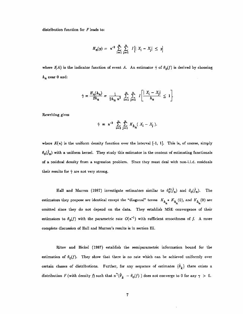
distribution function for F leads to:
where leA) is the indicator function of event A. An estimator i' of 00(/) is derived by choosing
hn near 0 and:
Rewriting gives
where K(u) is the uniform density function over the interval [-1, 1]. This is, of course, simply
0o(}n) with a uniform kernel. They study this estimator in the context of estimating functionals
of a residual density from a regression problem. Since they must deal with non-i.i.d. residuals
their results for i' are not very strong.
Hall and Marron (1987) investigate estimators similar to O;(}n) and 0o(}n)' The
estimators they propose are identical except the "diagonal" terms Kh * Kh (0), and Kh (0) aren n n
omitted since they do not depend on the data. They establish MSE convergence of their
estimators to 00(/) with the parametric rate O( n- l ) with sufficient smoothness of f. A more
complete discussion of Hall and Marron's results is in section III.
Ritov and Bickel (1987) establish the semiparametric information bound for the
estimation of 00(/)' They show that there is no rate which can be achieved uniformly over
certain classes of distributions. Further, for any sequence of estimates {Ok} there exists a
distribution F (with density fJ such that n'(Ok - 00(/) ) does not converge to 0 for any I > O.
7
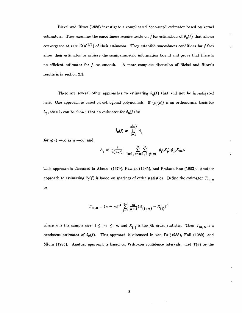
Bickel and Ritov (1988) investigate a complicated "one-step" estimator based on kernel
estimators. They examine the smoothness requirements on I for estimation of ()o(J) that allows
convergence at rate O( n-1/2) of their estimator. They establish smoothness conditions for I that
allow their estimator to achieve the semiparametric information bound and prove that there is
no efficient estimator for I less smooth. A more complete discussion of Bickel and Ritov's
results is in section 2.3.
There are several other approaches to estimating ()o(J) that will not be investigated
here. One approach is based on orthogonal polynomials. If {¢> i(x)} is an orthonormal basis for
L2, then it can be shown that an estimator for ()o(J) is:
lor q( n) --+00 as n --+00 and
This approach is discussed in Ahmad (1979), Pawlak (1986), and Prakasa-Rao (1983). Another
approach to estimating ()o(J) is based on spacings of order statistics. Define the estimator Tm n,
by
where n is the sample size, 1:5 m :5 n, and X(j) is the jth order statistic. Then Tm,n is a
consistent estimator of ()o(J). This approach is discussed in van Es (1988), Hall (1982), and
Miura (1985). Another approach is based on Wilcoxon confidence intervals. Let T(()) be the
8
Wilcoxon signed rank statistic, i.e.,
1'(0) = [n(n+l)jl 4:<L; I(X; + Xj > 20)'_J
where I(A) is the indicator of event A. If OLand 0U are the endpoints of the Wilcoxon
confidence interval then
is a consistent estimator of 0oU) for symmetric /. Aubuchon and Hettmansperger (1984) show
that this approach is asymptotically equivalent to the kernel-based method. Further results can
be found in Lehmann (1963).
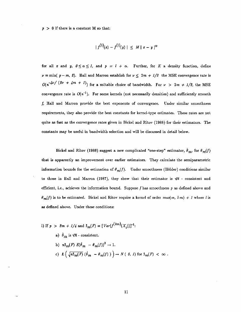
2.2) Estimating OIff) = J(f"(x)y dx
Estimating 0Iff) is an important problem in bandwidth selection for kernel density
estimates. A sensible approach to choosing the bandwidth hn is to choose it to minimize the
mean integrated square error (MISE) where MISE = EJU- h)2. Under some conditions
on K and f, MISE is minimized for
[ ]
1ft
~ ,.., n-1/ 5 JK
2
2 (Parzen, 1962).
{J ? K(x) dX} JU II) 2
Hence, estimation of 0Iff) is important for selecting a data-based bandwidth that is
asymptotically optimal. Of course, 0Iff) may be of interest simply as a measure of "curviness"
of a distribution.
9

Unlike the case of ()oU), there has not been much work devoted strictly to estimation of
()iJ). An exception is Wertz (1981), but his estimator is based on orthogonal series rather than
kernels. Much of the above work is generalized in Hall and Marron (1987) and Bickel and Ritov
(1988) to ()mU) for arbitrary m, and their results are discussed in section III.
2.3) Estimating ()mU) = J(/m)(x)Y dx, m arbitrary.
Most of the work on estimation of ()mU) is motivated by the previous two cases
(m = 0 and m = 2). There is usually little effort in extending mathematical results for "m = f!'
to "m finite". ()mU) for m > 2 does arise in the asymptotic investigations of some of the
estimators that will be studied here. The major difficulty in estimating ()mU) is that as m
becomes larger, BmU) requires more data for the same level of performance.
Hall and Marron (1987) generalize ();(}n) and ()o(}n) (discussed above) to arbitrary m.
The estimators they propose and investigate are:
and
Notice that these estimators omit the "diagonal terms", Le., the terms with i=j. These terms
do not depend on the data so they add a component to the estimator depending only on the
kernel shape and bandwidth. The effect of omitting these terms will be discussed below.
Hall and Marron investigate the MSE convergence of ()':n(}n) and () m(}n) to ()mU). The
rate of convergence depends on m and the smoothness of f The density f has smoothness
10
p > 0 if there is a constant M so that:
for all x and y, 05 a 51, and p = I + a. Further, for K a density function, define
II =min( p - m, 2). Hall and Marron establish for II 5 2m + 1/2 the MSE convergence rate is
O(n-411/ (211 + 4m + 1» for a suitable choice of bandwidth. For II > 2m + 1/2, the MSE
convergence rate is O(n- l ). For some kernels (not necessarily densities) and sufficiently smooth
J, Hall and Marron provide the best exponents of convergence. Under similar smoothness
requirements, they also provide the best constants for kernel-type estimates. These rates are not
quite as fast as the convergence rates given in Bickel and Ritov (1988) for their estimators. The
constants may be useful in bandwidth selection and will be discussed in detail below.
Bickel and Ritov (1988) suggest a new complicated "one-step" estimator, 8m, for 8m(f)
that is apparently an improvement over earlier estimators. They calculate the semiparametric
information bounds for the estimation of 8m (f). Under smoothness (Holder) conditions similar
to those in Hall and Marron (1987), they show that their estimator is '\f1i - consistent and
efficient, Le., achieves the information bound. Suppose f has smoothness p as defined above and
8m(f) is to be estimated. Bickel and Ritov require a kernel of order max(m, l-m) + 1 where I is
as defined above. Under these conditions:
a) 8m is '\f1i - consistent.
• 2b) n3m(F) E(8m - 8m(f» -+ 1.
c) L ( ~n3m(F) (Om - 8m(f) ) ) -+ N ( 0, 1) for 3m(F) < 00 •
11
ii) If m < p < 2m + 1/4,
a) E(Om - Om(f)2 = O(n-2"t) where 'Y =4(p • m)/{l + 4p)·
Further, they show that if p < 2m + 1/4 then their estimator achieves the best possible MSE
convergence rates. The proof that their estimator achieves the best possible convergence rate is
the main result of the paper. It is a surprising and important result that there should be a
changepoint in the convergence rate at 2m + 1/4.
12
Chapter II: Diagonal terms
1. Introduction.
The estimators discussed in this dissertation are of the form:
(2.1)
for some D which mayor may not be a function of the data. Notice that the "diagonal" terms
are omitted (although they may be included in D) so there are n( n - 1) terms in the summation.
The Hall and Marron estimators use D = O. The Sheather-Jones estimators use
D= n-1h-2m-1(_1)mI!2m)(O). Notice that this estimator is simply:
With an appropriate choice of the bandwidth, the Sheather and Jones estimators converge in
MSE faster than the Hall and Marron estimators because their D eliminates bias. Schweder
(1975) uses a data-based D aimed directly at eliminating bias for estimating 00(1).
Unfortunately, the Sheather-Jones work does not resolve the issue of whether or not to
include the diagonals in the estimator. It seems that there are two philosophical issues central
to this discussion. First, the diagonal terms are non-stochastic. Since the diagonal terms
depend only on the choice of bandwidth and kernel (i.e., not the data) it seems that they cannot
be a useful component of the estimator. It turns out that this position is just barely tenable,
but it seems fairly convincing at first glance. Second, including the diagonal terms forces the
estimator to be positive. This may not seem compelling; squaring the estimator or taking its
absolute value also make it positive. There is even some sense to allowing the estimator to be
negative. A negative value implies that the estimator does not have enough data to get a
reliable estimate of Om' A strictly positive estimator may provide a false sense of security in
what may be a nonsense estimate based on an impossibly small sample size (see chapter 6 for a
discussion of reasonable sample sizes). The benefits of a positive estimator stem more from
practical than philosophical considerations.
The practical issues involved in deciding whether or not to include the diagonals are
investigated throughout this dissertation, although usually in some other context. The purpose
of this chapter is to introduce and summarize many of those results. The diagonals decision is
the first choice a statistician must make in calculating a kernel estimate of Om' Even though
many of the results discussed here are not proven until later chapters, this choice justifies
including the results so early. The practical issues that will be addressed are bias reduction,
mean squared error, computation, and "stepped" estimation.
2. Bias Reduction.
If the positivity issue is ignored, then the reason for including the diagonal terms is that
with some clever choice of bandwidth including them eliminates some bias. Sheather and Jones
show that this causes a reduction in the asymptotic MSE of the estimator, compared to the
leave-out-the diagonals estimator. Basically, with a proper choice of bandwidth the diagonals
equal the first term in the Taylor expansion of the bias. This bandwidth is not so small that
the estimator is overwhelmed by variance, so the MSE is reduced.
Minus the positivity issue, this argument is not an adequate reason for using the leave
out-the-diagonals estimator. Bias reduction is fairly well-studied. If the only goal is to reduce
bias, then the limited approach of Sheather and Jones cannot be the best. It will be shown in a
14
later chapter that bias can be reduced (without affecting variance too much) by using a higher-
order kernel (Le., a symmetric kernel that is negative over some of its range), by using a more
sophisticated choice of D as in (2.1), or by "jackknifing". Any of these techniques can be used
to eliminate arbitrarily many terms in the Taylor expansion of bias. Unfortunately, with any of
these techniques the estimator is no longer necessarily positive.
3. Mean Squared Error Reduction.
Of course, a better goal than reducing bias is to reduce MSE. The Sheather-Jones
bandwidth is chosen only to reduce bias, although it clearly reduces MSE. An improved
estimator is suggested by choosing a data-based D to minimize the asymptotic MSE. The
following analysis suggests that choosing D this way results in an improved MSE convergence
rate.
Define (}m(in) as in (2.1). Extensions of calculations in Hall and Marron (1987) show
that:
where
15
In the three following cases, hAMSE is MSE asymptotically optimal bandwidth.
AMSE is simply the dominant terms in the expansion of MSE with the remainders disregarded. Case 1
is the Hall and Marron estimator, Case 2 is the Sheather and Jones estimator, Case 3 is the
general D.
Case 1: D = 0 (Hall and Marron)
1
hAMSE = ((-1 m + 1) C2)2r + 4m + 1
2r c; n2
..
A MSE(h ) - C n-1 + C n-2 h-4m- 1 +( C h2 )2AMSE - 1 2 3
1
where Al is a constant depending on K, m, and /.8
Hence, for Om(}n) with m =0, AMSE =C1 n-1 and for m =2, AMSE =Al n -13.
Case 2: (Sheather and Jones)
To eliminate the first term in the expansion of the bias choose ho so that
16
So
Notice that ho is not exactly the minimizer of AMSE. The real hAMSE for m ~ 1 would
minimize:
However, let hAMSE = CnC!L. Then the squared bias is at least O( n - 4/(2m+3») and this
minimum occurs at C!L = - 1/(2m + 3). Substitution shows that the variance is O( n - 5/(2m+3»)
at this minimum. Hence, ho '"" hAMSE as n-+oo. Finding the actual value of hAMSE requires
finding the real root of a (4m + 6)th order polynomial whose coefficients must be estimated.
Since this is difficult, we will say that hAMSE == ho and disregard the difference for a fixed value
of n.
Substituting ho into the expression for AMSE gives:
AMSE( hAMSE)
where A2 is a constant depending on K, m, and f. Hence, for 0m<Jn) with m = 0,
5AMSE= C1 n-1. For Om<Jn) with m = 2, AMSE= A2 n- 7
17
Notice that for estimating ()o(f) the convergence rates of the Hall and Marron estimator
is the same as that of the Sheather and Jones estimator. For estimating ()m(f), m ~ 1, the
Sheather and Jones estimator has a faster convergence rate. In particular, for m = 2, n-S/
7 is
£ -8~3a aster convergence rate than n .
Case 3: For general D,
Choose D = C3h2 to eliminate the first term in the bias and then choose h to mInimiZe
This gives:
1
_((4 m + 1) C2)4m + 9hAMSE - .J
8<.;, n24
A MSE(h ) - C n-I + C n-2 h-4m-1 + d h8AMSE - 1 2 4
2_ C -I + (C4 -8 C-4m- I )4m + 9 (__8_) 4m-~ 9 (4m + 9\- 1 n 2 n 4 4m + 1 4m + 1)
where A3 is a constant depending on K, r, and f. Hence, for () man) with m =0,16
AMSE = C1 n-I . For ()man) with m =2, AMSE = A3 n -17.
Notice that for estimating ()o(f) the convergence rates of this estimator is the same as
that of the Hall/Marron estimator and the Sheather/Jones estimator. For estimating ()m(f),
18
m;::: 1 this estimator has a faster convergence rate than the other two. In particular, for m = 2,
n-16/ 17 is a faster convergence rate than n-S/ 7 or n-S/
13• Some easy algebra shows for m;::: 1:
8 5 16o < 4m + 5 < 2m + 3 < 4m + 9 < 1.
For symmetric kernels and m > 0, the Hall and Marron estimator has the slowest MSE
convergence, followed by the Sheather and Jones estimator, and then the estimator using D
chosen to minimize the asymptotic MSE.
Despite the asymptotic results above, in practical estimation problems the D-estimator
does not always give better results than other kernel estimators. D must be estimated or
approximated and this added level of difficulty may overwhelm any asymptotic gains in
practical settings with even seemingly large sample sizes. As with all asymptotics, it is difficult
to predict when the sample size is large enough so that the asymptotic result applies.
A useful tool for gauging how well asymptotics work in fixed sample size cases is exact
MSE calculations with Normal mixture densities. Over any finite range, Normal mixture
densities can be shown to be dense withe respect to various norms in the space of all continuous
densities. Hence, most practical estimation problems can be approximated by using a Normal
mixture density as a test case. Details are provided in chapter V.
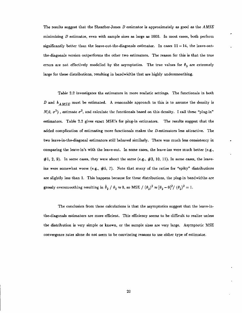
Table 2.1 provides some insight into how well the three estimators discussed above
perform. Fifteen Normal mixture densities are given in Appendix A. These densities seem to
be representative of a large class of densities that are likely to be encountered in a practical
estimation setting. For each density, the goal was to estimate 82, In each case, D and hAMSE
were calculated by assuming that the density was known. Of course, this is not realistic but still
provides some insights. The MSE's given are exact, based on calculations as described above.
19
The results suggest that the Sheather-Jones D estimator is approximately as good as the AMSE
minimizing D estimator, even with sample sizes as large as 1000. In most cases, both perform
significantly better than the leave-out-the-diagonals estimator. In cases 11 - 14, the leave-out
the-diagonals version outperforms the other two estimators. The reason for this is that the true
errors are not effectively modelled by the asymptotics. The true values for °3 are extremely
large for these distributions, resulting in bandwidths that are highly undersmoothing.
Table 2.2 investigates the estimators in more realistic settings. The functionals in both
D and hAMSE must be estimated. A reasonable approach to this is to assume the density is
N(O, 0-2 ) , estimate 0-
2 , and calculate the functionals based on this density. I call these "plug-in"
estimators. Table 2.2 gives exact MSE's for plug-in estimators. The results suggest that the
added complication of estimating more functionals makes the D-estimators less attractive. The
two leave-in-the-diagonal estimators still behaved similarly. There was much less consistency in
comparing the leave-in's with the leave-out. In some cases, the leave-ins were much better (e.g.,
#1, 2, 9). In some cases, they were about the same (e.g., #3, 10, 11). In some cases, the leave
ins were somewhat worse (e.g., #5, 7). Note that many of the ratios for "spiky" distributions
are slightly less than 1. This happens because for these distributions, the plug-in bandwidths are
grossly oversmoothing resulting in 02 / °2 ~ 0, so MSE / (82)2 ~ [82 - 0]2/ (82)2 = 1.
The conclusion from these calculations is that the asymptotics suggest that the leave-in
the-diagonals estimators are more efficient. This efficiency seems to be difficult to realize unless
the distribution is very simple or known, or the sample sizes are very large. Asymptotic MSE
convergence rates alone do not seem to be convincing reasons to use either type of estimator.
20
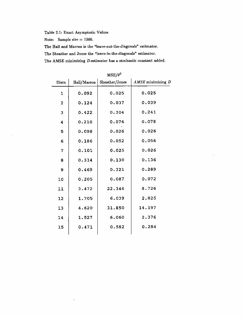
Table 2.1: Exact Asymptotic Values
Note: Sample size = 1000.
The Hall and Marron is the "leave-out-the-diagonals" estimator.
The Sheather and Jones the "leave-in-the-diagonals" estimator.
The AMSE minimizing D-estimator has a stochastic constant added.
MSE/0 2
Distn Hall/Marron Sheather/Jones AMSE minimizing D
1 0.092 0.025 0.025
2 0.124 0.037 0.039
3 0.422 0.304 0.241
4 0.210 0.076 0.078
5 0.098 0.026 0.026
6 0.186 0.052 0.056
7 0.101 0.025 0.026
8 0.314 0.130 0.136
9 0.469 0.321 0.289
10 0.205 0.087 0.072
11 3.472 22.346 8.726
12 1.705 6.039 2.825
13 4.620 31.850 14.197
14 1. 527 6.060 2.376
15 0.471 0.582 0.284
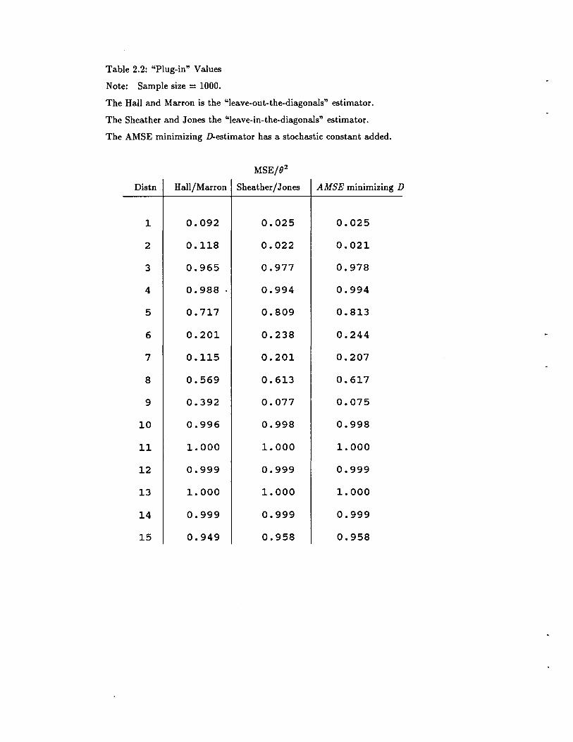
Table 2.2: "Plug-in" Values
Note: Sample size = 1000.
The Hall and Marron is the "leave-out-the-diagonals" estimator.
The Sheather and Jones the "leave-in-the-diagonals" estimator.
The AMSE minimizing D-estimator has a stochastic constant added.
MSE/(}2
Distn Hall/Marron Sheather/Jones AMSE minimizing D
1 0.092 0.025 0.025
2 0.118 0.022 0.021
3 0.965 0.977 0.978
4 0.988 0.994 0.994
5 0.717 0.809 0.813
6 0.201 0.238 0.244
7 0.115 0.201 0.207
8 0.569 0.613 0.617
9 0.392 0.077 0.075
10 0.996 0.998 0.998
11 1. 000 1. 000 1. 000
12 0.999 0.999 0.999
13 1. 000 1. 000 1. 000
14 0.999 0.999 0.999
15 0.949 0.958 0.958
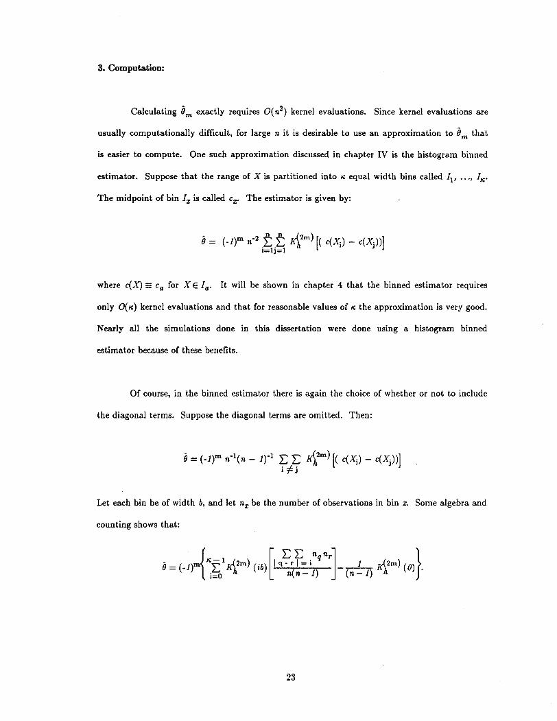
3. Computation:
Calculating Om exactly requires O(n2 ) kernel evaluations. Since kernel evaluations are
usually computationally difficult, for large n it is desirable to use an approximation to Om that
is easier to compute. One such approximation discussed in chapter IV is the histogram binned
estimator. Suppose that the range of X is partitioned into", equal width bins called II' ..., I",.
The midpoint of bin Ix is called cx. The estimator is given by:
where c(X) == ca for X E Ia. It will be shown in chapter 4 that the binned estimator requires
only 0(",) kernel evaluations and that for reasonable values of", the approximation is very good.
Nearly all the simulations done in this dissertation were done using a histogram binned
estimator because of these benefits.
Of course, in the binned estimator there is again the choice of whether or not to include
the diagonal terms. Suppose the diagonal terms are omitted. Then:
Let each bin be of width b, and let nx be the number of observations in bin x. Some algebra and
counting shows that:
{
",-I [ E E .nqnrJ }0= (_l)rn E T)2rn) (ib) I q- r 1= 1 __1_ T)2rn) (0) .i=oL\h n(n-1) (n_1)L\h
23
An eliminator of non-stochastic terms would now drop the last term giving:
However, the same counting and algebra done in reverse shows that this is equal to:
the binned estimator with the diagonals left in.
This may not contribute greatly to the discussion of whether or not to include the
diagonals in the unbinned estimator, but it seems to resolve it in the case of the binned
estimator. The leave-out-the-diagonals estimator may be negative and it includes a non-
stochastic term. The leave-in-the diagonals estimator is positive and has no non-stochastic
terms.
4. "Stepped" estimators.
As shown in section 2, the asymptotically optimal bandwidths for estimating Om are all
functions of 0m+l' In chapters VII and VIII, multi-step estimators will be discussed in which
0m+k is estimated to arrive at an estimated optimal bandwidth for Om' In this setting, the
positivity of the leave-in-the-diagonals estimator is absolutely necessary. Results about these
kinds of estimators will be discussed in depth in these later chapters.
24
Chapter ill: Bias Reduction
1. Introduction.
From Hall and Marron (1987), the estimator defined in (2.1) with D = 0 is biased. The
Sheather and Jones estimator discussed in chapter 2, adds a component which cancels some of
this bias. The result is an estimator with a faster MSE convergence rate. The natural question
is whether some further bias reduction might eliminate more bias and result in even faster MSE
convergence rates (or, more modestly, with the same MSE convergence rate but a better
constant).
The Sheather-Jones approach is basically to add something to the estimator to cancel a
term in the Taylor expansion of the bias. Of course, the obvious extension is to add something
different to cancel the first several terms in the bias. These estimators wll be called
D - estimators.
Three approaches to reducing bias in kernel estimates are higher order kernels, D
estimates, and the generalized jackknife. This section will examine each of these approaches and
establish the connections between them. The generalized jackknife and the higher order kernel
estimates are equivalent. A D-estimate is a higher order kernel estimate. Under some
conditions (stated below), a higher order kernel or generalized jackknife estimate can be written
as aD-estimate.
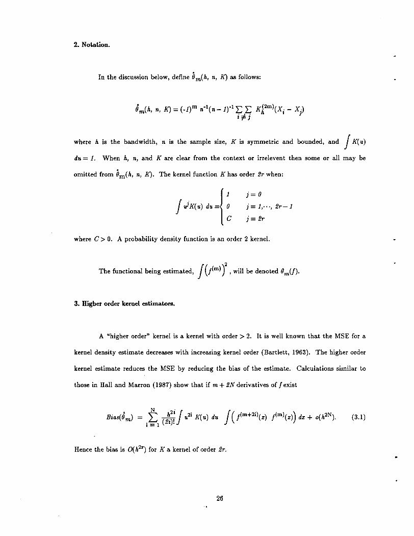
2. Notation.
In the discussion below, define Om(h, n, K) as follows:
Om(h, n, K) = (_l)m n- l (n-1rl ~):; K~2m)(Xi - X)I r1
where h is the bandwidth, n is the sample size, K is symmetric and bounded, and JK( u)
du = 1. When h, n, and K are clear from the context or irrelevent then some or all may be
omitted from Om(h, n, K). The kernel function K has order 2r when:
j= 0
j = 1,.··, 2r-1
j= 2r
where C> O. A probability density function is an order 2 kernel.
The functional being estimated, J(im)Y,will be denoted Bm(J)·
3. Higher order kernel estimators.
A "higher order" kernel is a kernel with order> 2. It is well known that the MSE for a
kernel density estimate decreases with increasing kernel order (Bartlett, 1963). The higher order
kernel estimate reduces the MSE by reducing the bias of the estimate. Calculations similar to
those in Hall and Marron (1987) show that if m + 2N derivatives of f exist
Hence the bias is O(h2r) for K a kernel of order 2r.
26
In kernel density estimation, this smaller MSE has a price. Since a higher order kernel
must have negative values, the interpretation of the density estimate as a moving weighted
•average is obscured. For estimating ()mU), an added problem is that ()m(h, n, K) may be
negative for higher order K even though ()m(/) is positive. Nevertheless, the lower MSE may be
attractive.
4. lHstimators.
A straightforward technique for reducing bias is to subtract an estimate of the bias from
the estimate of ()mU). This allows a probability density kernel to be used, preserving the
moving average interpretation of the density estimate. If K is a density, then the first order
bias term of 0m(K) is
To reduce the bias In Bm(K), this bias term may be estimated and subtracted from Bm(K).
Define
(3.2)
former will be called a D-estimator.
The disadvantage of this technique is that another estimation problem has been added
to an already difficult problem. Instead of selecting one kernel and bandwidth, two are required.
A more general version of a D-estimator may include terms to eliminate higher order bias terms
and these add still more estimation problems.
27
5. Generalized jackknife estimators.
• •Let (}m(hv nl , KI ) and (}m(h2, n2' K2) be distinct estimates of (}mU). For simplicity
suppose that KI and K2 are densities, although this is not required in the general case. Define
Using the expression for bias given in (3.1),
The first-order bias term is eliminated if
R=hI
2Ju2 K1( u) du
h/ Ju2 K2(u) du·
The estimator qOm(hv nl , KI ), Om(h2 , ~, K2), R) with R chosen this way is called a
generalized jackknife estimator (for a similar discussion of density estimation see Schucany and
Sommers, 1977).
The difficulty with the generalized jackknife is similar to the difficulty with the D-
estimator; the improved bias costs another estimation problem. It is also not clear how the two
estimators should be chosen in relation to each other.
28
For a discussion of how the generalized jackknife relates to the more common
"pseudovalue" jackknife see Gray and Schucany (1972).
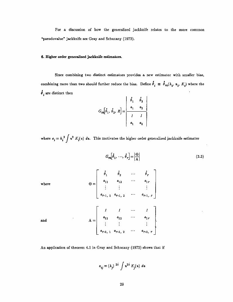
6. Higher order generalized jackknife estimators.
Since combining two distinct estimators provides a new estimator with smaller bias,
• •combining more than two should further reduce the bias. Define (J i == (J m(hi' ni' Ki) where the
•(J i are distinct then
where ai = h/Ju2 K j ( u) duo This motivates the higher order generalized jackknife estimator
where
and
J' .] lei (3.3)G (JI'···' (Jr = iAi
• • •(JI (J2 (Jr
e=an aI2 aIr
ar - I , I ar _l , 2 ar _l , r
1 1 1
A=an aI2 aIr
ar _l , I ar - I , 2 ar _l , r
An application of theorem 4.1 in Gray and Schucany (1972) shows that if
29
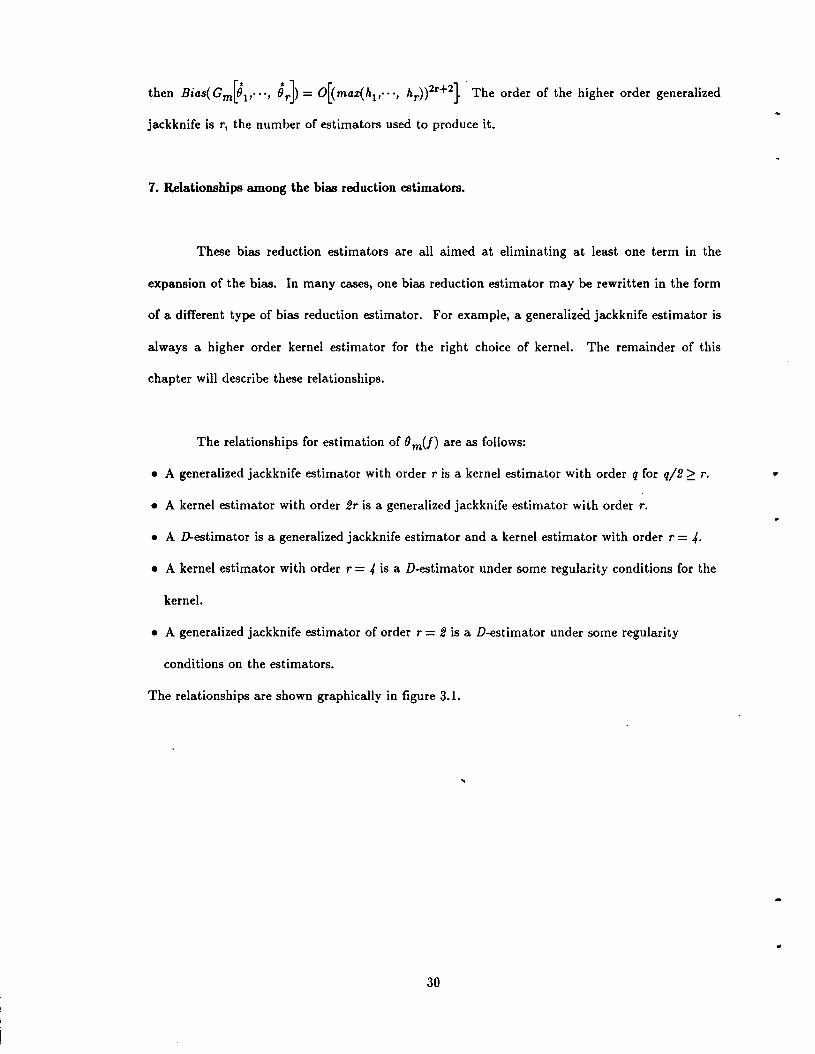
then Bias(Gm[0l"'" Or]> = O[(max(h1,···, hr))2r+2}· The order of the higher order generalized
jackknife is r, the number of estimators used to produce it.
7. Relationships among the bias reduction estimators.
These bias reduction estimators are all aimed at eliminating at least one term in the
expansion of the bias. In many cases, one bias reduction estimator may be rewritten in the form
of a different type of bias reduction estimator. For example, a generalized jackknife estimator is
always a higher order kernel estimator for the right choice of kernel. The remainder of this
chapter will describe these relationships.
The relationships for estimation of () m(J) are as follows:
• A generalized jackknife estimator with order r is a kernel estimator with order q for q/22: r.
• A kernel estimator with order 2r is a generalized jackknife estimator with order r.
• A D-estimator is a generalized jackknife estimator and a kernel estimator with order r = 4.
• A kernel estimator with order r = 4 is a D-estimator under some regularity conditions for the
kernel.
• A generalized jackknife estimator of order r = 2 is a D-estimator under some regularity
conditions on the estimators.
The relationships are shown graphically in figure 3.1.
..
30
•
..
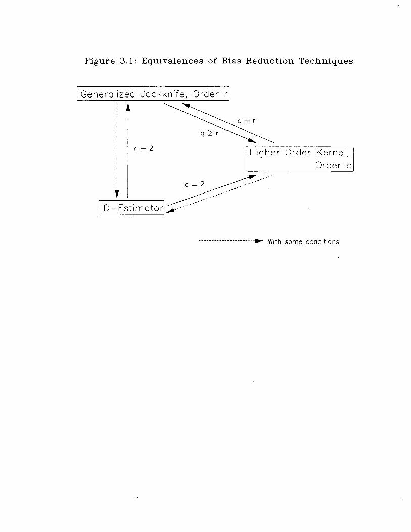
Figure 3.1: Equivalences of Bias Reduction Techniques
I Generalized Jackknife, Order rl
r = 2
,0- Estimatorl .....----------
Higher Order Kernel,
Order q
______________ n ~ With some conditions
8. Theorems.
The first two theorems show the equivalence of the generalized jackknife and the higher
order kernel estimators.
Theorem 3.1: A generalized jackknife estimator of order r is a higher order kernel estimator of
order q, where q/2 ~ r if each lJ i in the generalized jackknife estimator is based on all n
observations.
Proof: The proofs of all theorems in this chapter are given in Section 10.
For an example of a higher order kernel estimate of degree q where q/2 > r where r is
the degree of the equivalent jackknife estimator see Schucany and Sommers (1977). The
example they give is for density estimation but it is easily extended.
Theorem 3.2: A higher order kernel estimator of order 2r is a generalized jackknife estimator of
order r.
The next theorem shows that a D-estimator is a second order kernel estimator, and by
the previous two theorems, a second order generalized jackknife estimator. The theorem
provides the construction of the fourth order kernel. A construction of the equivalent
generalized jackknife kernels is given in the proof of theorem 3.2.
32
"
..
•
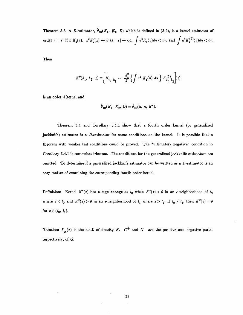
Theorem 3.3: AD-estimator, 8m(KI , .((2' D) which is defined in (3.2), is a kernel estimator of
order r=4 ifxK2(x), x'2K;(x) -+ Oas Ixl-+ 00, Ju4 KI (u)du < 00, and Ju4 KP)(u)du<00.
Then
is an order 4 kernel and
Theorem 3.4 and Corollary 3.4.1 show that a fourth order kernel (or generalized
jackknife) estimator is a D-estimator for some conditions on the kernel. It is possible that a
theorem with weaker tail conditions could be proved. The "ultimately negative" condition in
Corollary 3.4.1 is somewhat irksome. The conditions for the generalized jackknife estimators are
omitted. To determine if a generalized jackknif~ estimator can be written as a D-estimator is an
easy matter of examining the corresponding fourth order kernel.
Definition: Kernel K*(x) has a sign change at to when K*(x) < 0 in an f-neighborhood of to
where x < to and K*(x) > 0 in an f-neighborhood of tl where x> tl . If to::ft tll then K*(x) = 0
Notation: F~x) is the c.d.f. of density K. a+ and a- are the positive and negative parts,
respectively, of G.
33
Theorem 3.4: If K"'(x) has order 4, has 2 sign changes, and K"'(x) is o(x-3) as 1x 1- 00 then
where
In the above construction, a single bandwidth is used for both kernels. Since a
D-estimator may have different ,bandwidths for each kernel, a more general result is available
than the theorem.
Corollary 3.4.1: If K"'(x) has order 4, is ultimately negative and o(x-3 ) as I x 1- 00, and
K"'(x) > 0 in a neighborhood of 0, then O(h, n, K"') can be written as aD-estimator.
9. Example.
The following example shows one estimate written as a D-estimate, a generalized
jackknife estimate, and a second order kernel estimate. The functional being estimated is J/2
where / is the Normal mixture distribution #2 given in Appendix A.
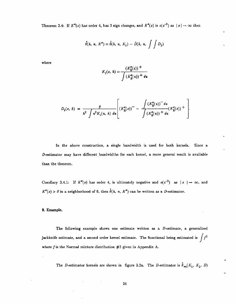
The D-estimator kernels are shown in figure 3.2a. The D-estimator is Bm(K1 , K2 , D)
34
where D =D(hl , h2 , n, K1, K2 ), hI =0.189, h2 =0.347, n =250, and Kl' K2 are standard
Gaussian densities. The bandwidths are MSE optimal.
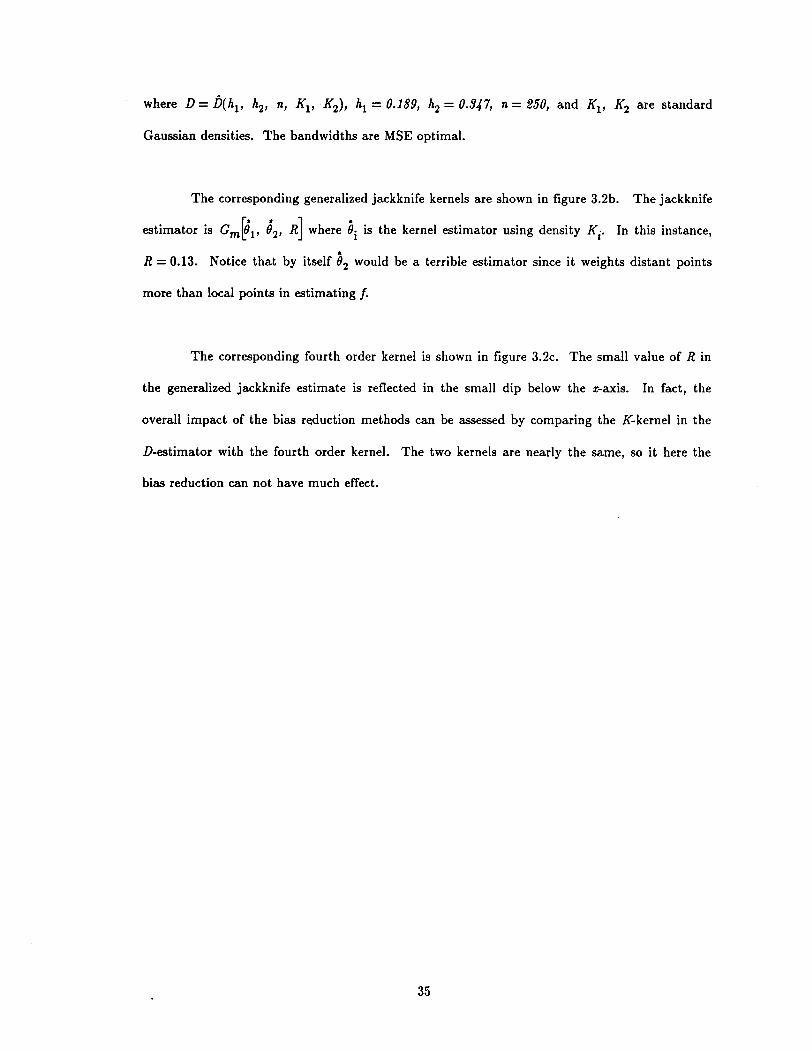
The corresponding generalized jackknife kernels are shown in figure 3.2b. The jackknife
estimator is Gm~l' 82, R] where 0i is the kernel estimator using density Ki. In this instance,
R =0.13. Notice that by itself O2 would be a terrible estimator since it weights distant points
more than local points in estimating f.
The corresponding fourth order kernel is shown in figure 3.2c. The small value of R in
the generalized jackknife estimate is reflected in the small dip below the x-axis. In fact, the
overall impact of the bias reduction methods can be assessed by comparing the K-kernel in the
D-estimator with the fourth order kernel. The two kernels are nearly the same, so it here the
bias reduction can not have much effect.
35
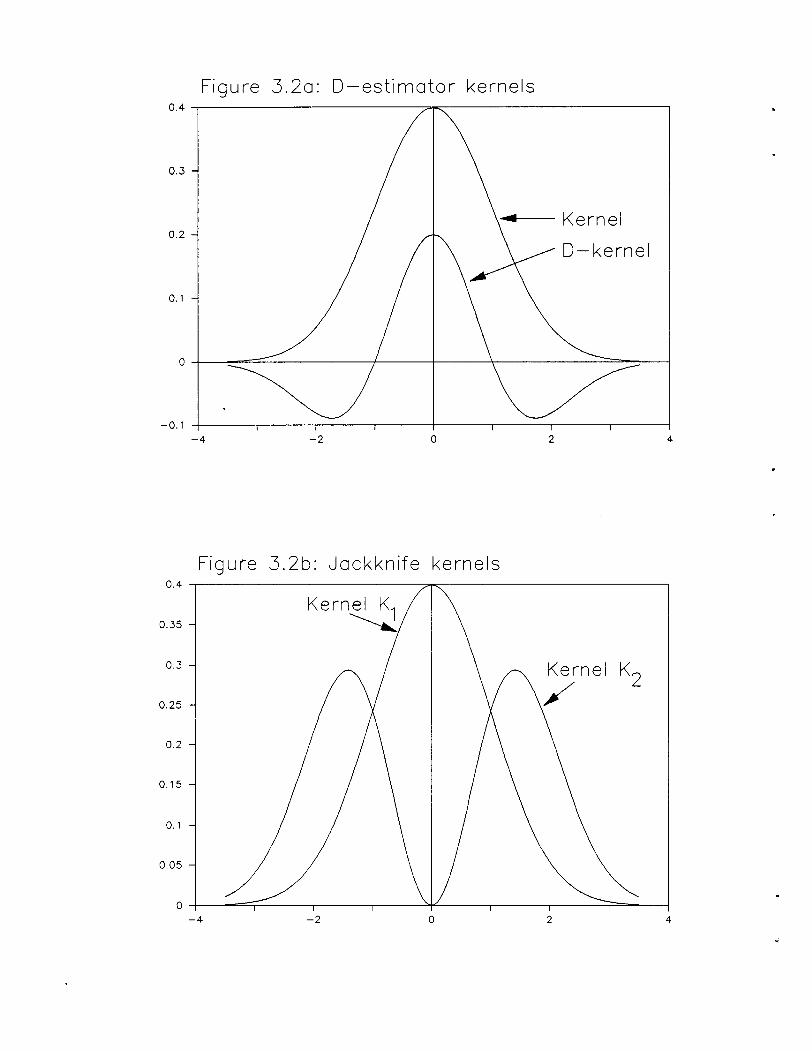
Figure 3.20: D-estimator kernels0.4 -.------------~~----------___,
0.3
, ....1--- Kernel0.2
0.1
O+-~--==----____tL--__+--__\_--------==~____l
-0.1 -+---,-----,-------,----+------,-----,-------r-------j
-4 -2 o 2 4
Figure 3.2b: Jackknife kernels0.4
0.35
0.3 K2
0.25
0.2
0.15
0.1
0.05
0-4 -2 0 2 4
Figure 3.2c: Second-order kernel0.6
0.5
0.4
0.3
0.2
0.1
0
-0.1-4 -2 0 2 4
10. Proofs.
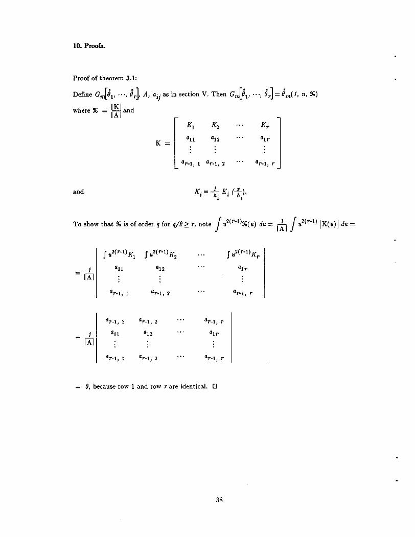
Proof of theorem 3.1:
Define OJOl' "', ,q, A, aij as in section V. Then OJOl' "', Or] = 0m(1, n, %)
IKIwhere 9G = iAl and
K=
and
To show that % is of order q for q/2 ~ r, note Ju2(r-I)%( u) du = 111 Ju2(r-I) IK( u) Idu =
Ju2(r-I) KI
Ju2(r-I) K2
Ju2(r-I) Kr
1 an aI2 aIr= iAl
ar-I , I ar_I , 2 ar_I, r
ar_I , I ar_I , 2 ar_I, r
1 an al2 aIr= iAl
ar_I , I ar-I , 2 ar_I , r
= 0, because row 1 and row r are identical. 0
38
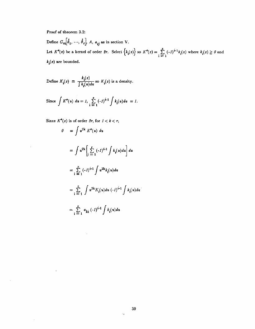
Proof of theorem 3.2:
Define aJOl' "', Orl A, aij as in section V.
Let K*(x) be a kernel of order 2r. Select {ki(x)} so K*(x) = .t (-1)i-1ki(x) where ki(x) ~ 0 and1=1
ki(x) are bounded.
Define Ki(x)k,{x) . .
- I ki(u)du so Ki(x) IS a density.
Since JK*( u) du =1, . t (_1)i-l Jki(u)du =1.1=1
Since K*(x) is of order 2r, for 1 < k < r,
o = Ju2k K*(u) du
39
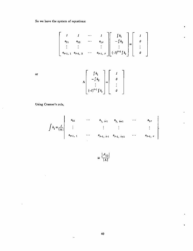
So we have the system of equations:
1 1 1 I k1 1
an au aIr -I~ 0=
ar_1, 1 ar_1, 2 ar_1, r (_l)r-l I kr 0
or I k1 1
- I k2 0A =
(_l)r-l I kr 0
Using Cramer's rule,
an aI, i-I aI, i+l aIr
Jki =ll lar_1, 1 a . ar_1, i+l ar_1, rr-l, ,-I
40
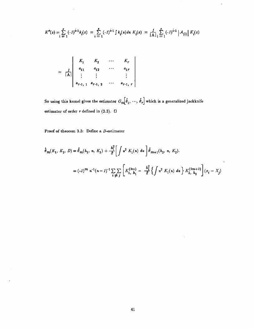
K*(x) = t (-l)i- I ki(x) = t (-l)i- I Jk{u)duK{x) = IA1 11.L:=rI(-1)i-I I.A(i)IKi(x)
i=I i=I I I
KI K2 Kr
1 an aI2 aIr= iAi
ar _I , 1 ar_I, 2 ar_I, r
So using this kernel gives the estimator GJOI' "', Or] which is a generalized jackknife
estimator of order r defined in (3.3). 0
Proof of theorem 3.3: Define a D-estimator
41
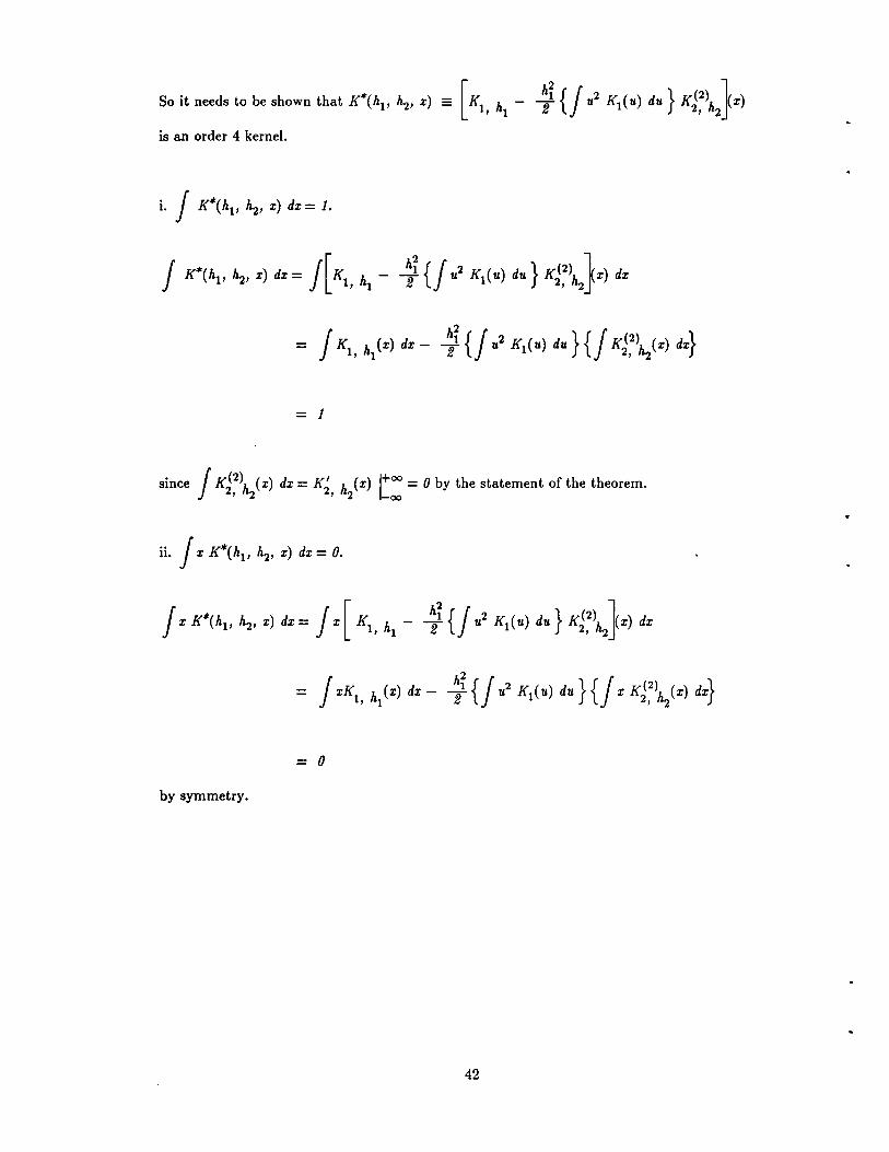
So it needs to be shown that K*(hI, h2 , x) - [KI, hI - ~~ {J u2 KI(u) du } KJ:)h2}X)
is an order 4 kernel.
= 1
since JKJ2)h (x) dx =K; h (x) 1+00 =0 by the statement of the theorem., 2 ' 2 -00
= 0
by symmetry.
42
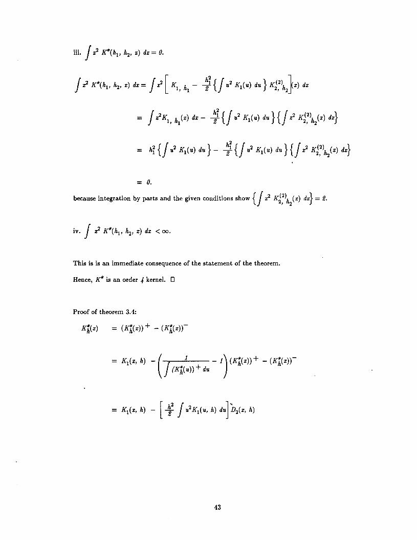
= o.
because integration by parts and the given conditions show {J 1? KJ:>h.z(x) dX} = 2.
This is is an immediate consequence of the statement of the theorem.
Hence, K* is an order 4 kernel. 0
Proof of theorem 3.4:
43
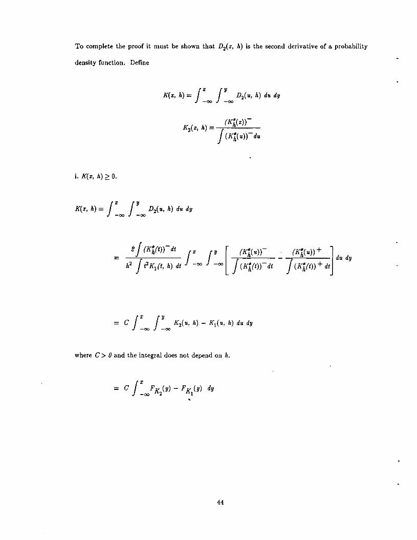
To complete the proof it must be shown that D2(x, h) is the second derivative of a probability
density function. Define
i. K(x, h) ~ O.
. (K*(u))+ J- h du dyJ(Ki/t)) + dt
where C> 0 and the integral does not depend on h.
..
44
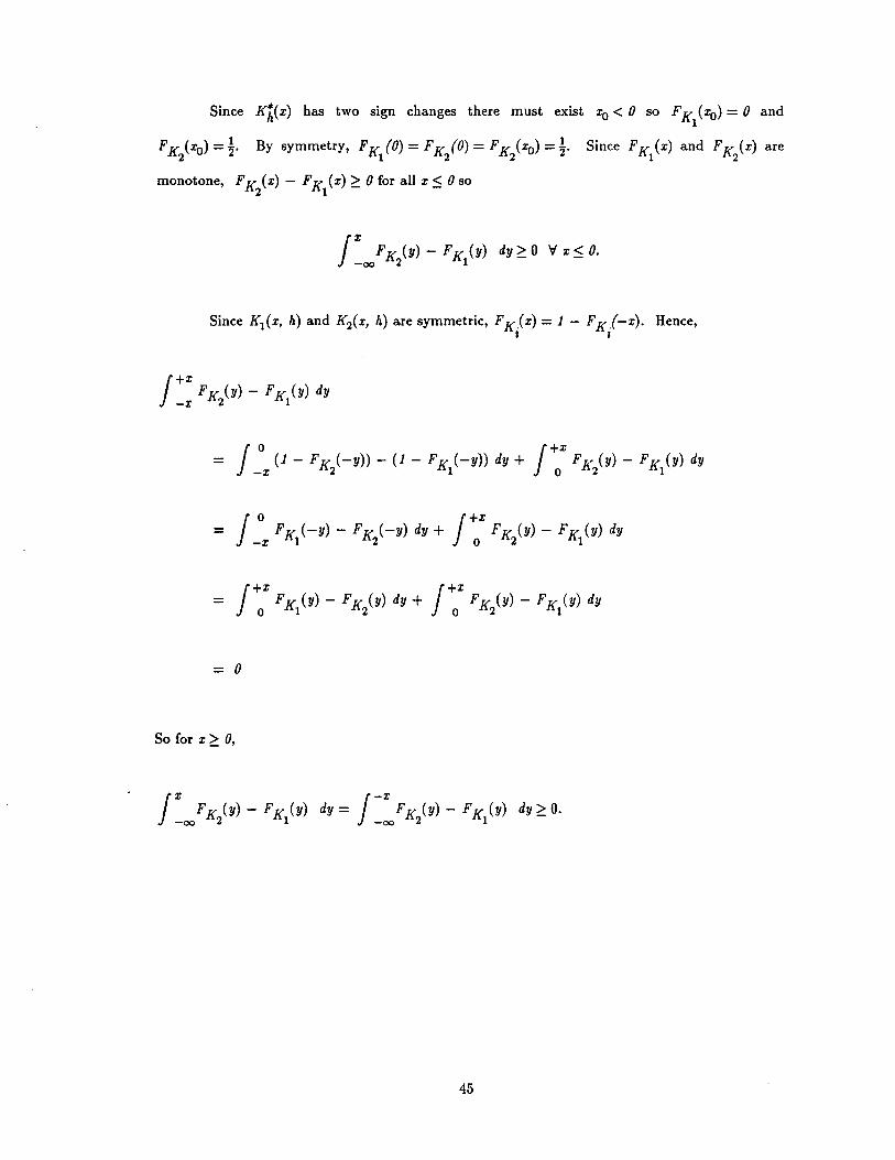
Since Kh(x) has two sign changes there must exist Xo < 0 so FK (xo) = 0 and1
FK (xo) =~. By symmetry, FK (0) = FK (0) = FK (xo) =~. Since FK (x) and FK (x) are2 1 2 2 1 2
monotone, FK/x) - FK/x);::: 0 for all x:5 0 so
Jx FK (y) - FK (y) dy;::: 0 V x:5 o.-00 2 1
Since K1(x, h) and K2(x, h) are symmetric, FK(x) = 1 - FKI-x). Hence,I I
J+xFK (y) - FK (y) dy
-x 2 1
= J 0 (1- FK (-y)) - (1- FK (-y)) dy + J+x FK (y) - FK (y) dy-x 2 1 0 2 1
= J 0 FK (-y) - FK (-y) dy + J+x FK (y) - FK (y) dy-x 1 2 0 2 1
= J+x FK (y) - FK (y) dy + J+x FK (y) - FK (y) dyo 1 2 0 2 1
= 0
So for x;::: 0,
45
ii. K( x, h) is integrable.
By symmetry, it suffices to show /:00 / ~oo /:00 K2( w) dw du dy < 00. Since
K*(x) is 0(x·3 ), K2(x, h) is 0(x·3 ). Since K*(x) is an order 4 kernel, /:00~ K2( w) dw < 00.
Two applications of integration by parts using K2(x, h) being 0(x·3 ) proves the result.
/+00
iii. K(x, h) dx = 1.-00
By Hall and Marron (1987) and integration by parts,
E [8(h, n, K*)] - 8 = ~; ( / (!"(x) r dx )(/ u4 K*(u) dU) + 0(h4).
. -E [8(h, n, K1 ) - D(h, n, K)] - 8 =
- ~2 ( / (f'(x)) 2 dx )(/ u2 K1(u, h) dU) - E [D(h, n, K)] + 0(h2).
Since E [8(h, n, K*)] = E [8(h, n, K1) - D(h, n, K)] and matching terms in the expansion,
E [D(h, n, K)] = - ~2 ( J(!'(x) r dx )(J u2 K1(u, h) dU) + 0(h2).
So by the definition of D,
E [KA2 )(xi - X)] = - ( J(f'(x) r dx ) + 0(1).
46
However from Hall and Marron (1987),
E [Kh2 )(xi - Xj)] = - / / K(u, h) f'(x) f'(x - hu) dx du
= -[(I K(u, h) dU)( / (f'(x) f dX) + 0(1)]
This implies / K( u, h) du = 1.
This completes the proof of the theorem. 0
Proof of Corollary 3.4.1:
Suppose K*(x) ~ 0 for I x I > a and a is a sign change point. Further, suppose K*(x) 2:: 0 for
I x I < band b is a sign change point.
Let K**(x) = +[K*] + (+x) - [K*]-(x).
Then K**(x) meets the conditions of the previous theorem and may be written as a D-
estimator according to the construction given there. So, using the same definitions as in the
theorem, if
• **' . / /O(h, n, K ) = O(h, n, Kt ) - D(h, n, D2 )
then
• *' bh • / /O(h, n, K ) =O(-a-' n, Kt ) - D(h, n, D2 ). 0
47

Chapter IV: Computation
1. Introduction.
The basic estimator, defined in (2.1), is a double sum requiring O( n2 ) kernel
evaluations. For reasonable values of n, the computation time for the estimator is "feasible".
For many of the applications discussed in this dissertation, however, the computation time
required for straightforward calculation is a burden. For example, the "k - step" estimators
discussed in Chapter VIII require O(k x n2 ) kernel evaluations to calculate directly. Even on a
relatively fast computer, simulations which require many repetitions of this operation can take
weeks to finish.
This chi;l.pter discusses a computation strategy called "binning" to reduce the
computation time by approximating the estimator. The object of binning is to distribute the
data initially to II "bins". The estimator is computed on the "binned" data. The pay-off is that
the estimator now requires only 0(11) kernel evaluations.
The simplest binning is called "histogram" binning. The range of the data is divided
into II equal width bins. Each observation is recoded to equal the midpoint of the bin in which
it lies. The estimator is calculated using the recoded data instead of the original data.
A more complicated type of binning is called "generalized" binning. The range of the
data is similarly partitioned into II bins as in histogram binning. The new data consists of a
kernel density estimate at each bin midpoint. A special case discussed below is "linear" binning
in which the kernel for the generalized binning is a triangular kernel.
There are two questions that are addressed in this chapter: "How should the data be
binned?" and "How much error is introduced by the binning?". These questions are answered
with asymptotic calculations. In general, bin widths slightly smaller than the bandwidth seem
to give good results and require much less computation time.
2. Notation:
In the discussion below, assume that there are v bins of width b. The bins are called
Iv "', Iv· The midpoint of bin Ia will be denoted ca and c(x) == ca if x is in bin a.
Define 0m as follows:
Define 0m(h, n, K) as follows:
Om(h, n, K)
where h is the bandwidth, n is the sample size, K is a symmetric, bounded probability density
function. Define 8m(h, n, K) as follows:
•0m(h, n, K) (./.1)
where 9 is some function of the observations. When h, n, and K are clear from the context or
irrelevant then some or all may be omitted from Om(h, n, K) or 8m(h, n, K).
49
3. The histogram binned estimator.
The histogram binned estimator is the most straightforward type of binning. That is:
•0m(h, n, K)
where c(X) == ca if X E fa and c(X) == 0 otherwise. In the notation of (4.1):
where na is the number of observations in bin a.
Lemma 4.1 provides the asymptotic variance and squared bias for Bm(h, n, K) as
h, 6 -+ 0; n -+ 00; nh, n6-+00. It is similar to lemma 3.1 in Hall and Marron (1987).
Lemma 4.1: For f a density with a continuous (m + 1)5t derivative vanishing at ± 00, and K a
symmetric infinitely differentiable kernel:
. ' 2 2 [h4 {I 2 }2 64
] 4 41. {E[ (}m(h, n, K) - Om]} = Om+! T u K(u) du + 144 + 0(6 ) + o(h ).
50
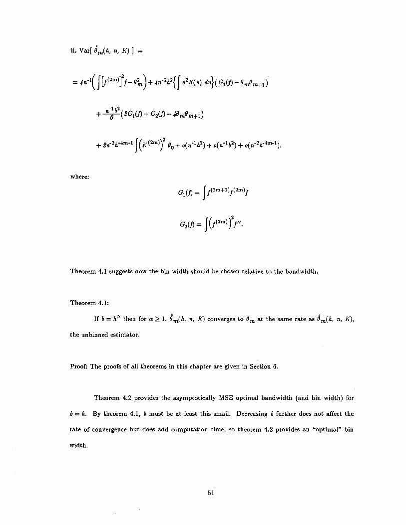
•ii. Var[ 0m(h, n, K)] =
where:
Theorem 4.1 suggests how the bin width should be chosen relative to the bandwidth.
Theorem 4.1:
If b= h(k then for a 2= 1, Om(h, n, K) converges to Om at the same rate as Bm(h, n, K),
the unbinned estimator.
Proof: The proofs of all theorems in this chapter are given in Section 6.
Theorem 4.2 provides the asymptotically MSE optimal bandwidth (and bin width) for
b = h. By theorem 4.1, b must be at least this small. Decreasing b further does not affect the
rate of convergence but does add computation time, so theorem 4.2 provides an "optimal" bin
width.
51
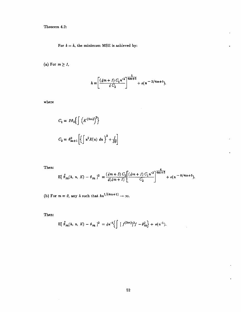
Theorem 4.2:
For b= h, the minimum MSE is achieved by:
(a) For m ~ 1,
where
Then: 4
E[ 0 (h K) _ 8 ]2 _ (4m+ 5) C2 [(4m+ 1) C1n-2]4m+5 (-S/4m+5)
m ,n, m - 4(4m + 1) C2
+ 0 n .
(b) For m = 0, any h such that hnl /(4m+l) --. 00.
Then:
52
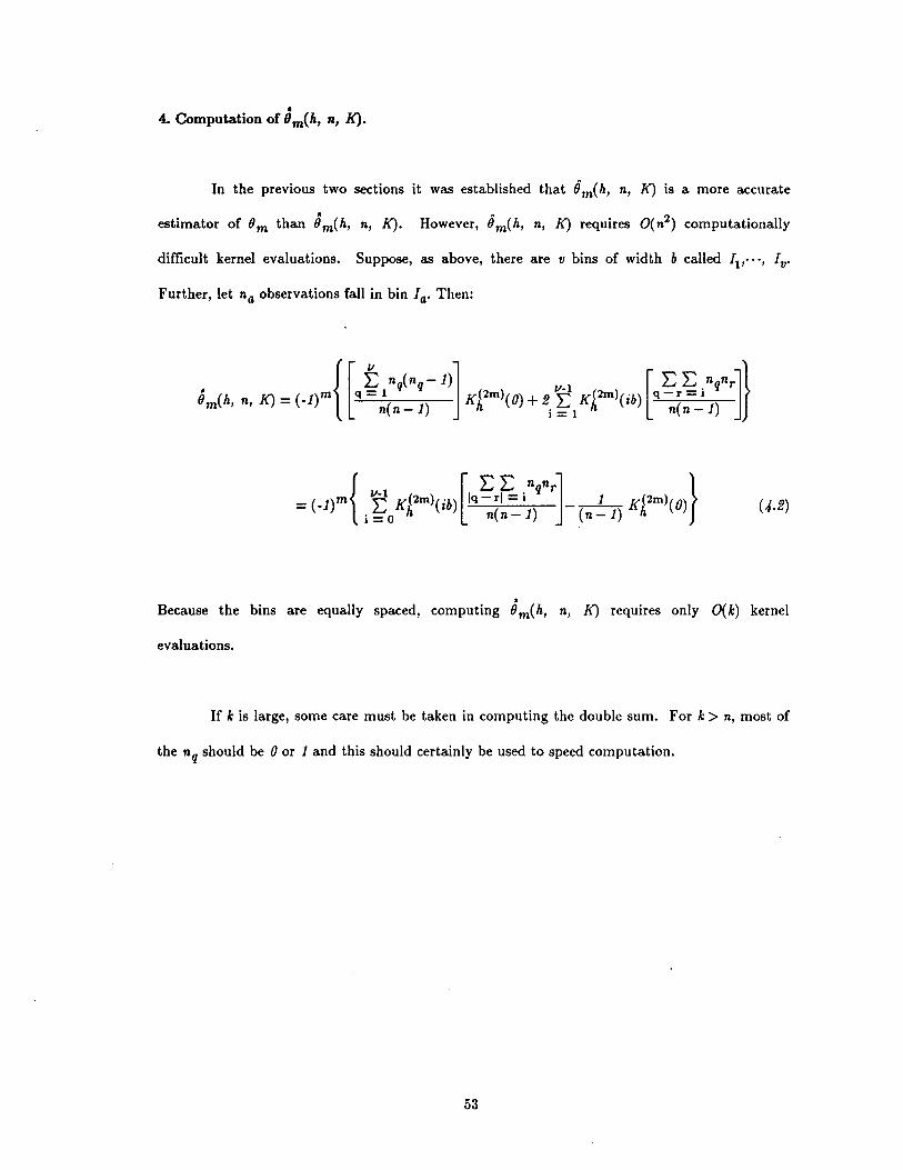
•4. Computation of 0m(h, n, K).
In the previous two sections it was established that (j m( h, n, K) is a more accurate
estimator of 8m than 8m(h, n, K). However, 8m(h, n, K) requires O(n2) computationally
difficult kernel evaluations. Suppose, as above, there are v bins of width b called II"'" Iv.
Further, let na observations fall in bin I a• Then:
=(_J)m{ ~ K(2m)(ib)[lq~r~inqnr] __1_K(2m)(o)} (4.2)i = 0 h n( n - 1) (n - 1) h
Because the bins are equally spaced, computing 8m(h, n, K) requires only O(k) kernel
evaluations.
If k is large, some care must be taken in computing the double sum. For k> n, most of
the nq should be 0 or J and this should certainly be used to speed computation.
53
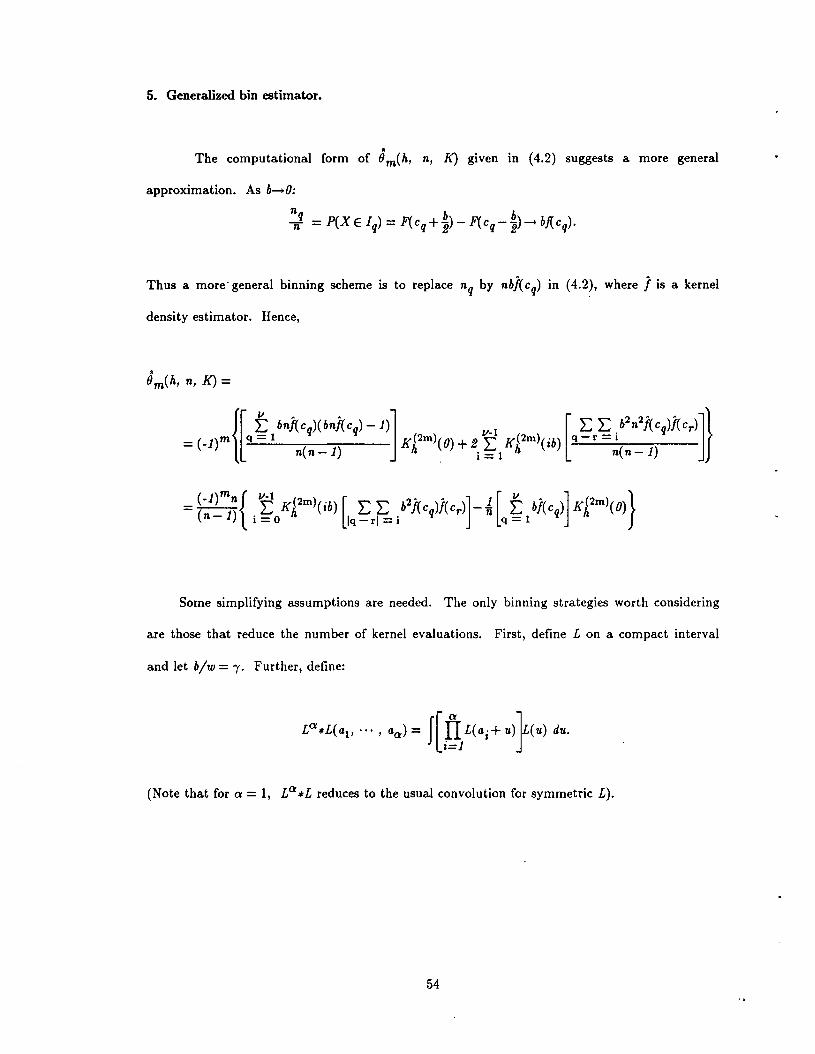
5. Generalized bin estimator.
The computational form of Om(h, n, K) given in (4.2) suggests a more general
approximation. As b-+O:
Thus a more' general binning scheme is to replace nq by nbj( cq) In (4.2), where j is a kernel
density estimator. Hence,
Some simplifying assumptions are needed. The only binning strategies worth considering
are those that reduce the number of kernel evaluations. First, define L on a compact interval
and let b/w ={' Further, define:
(Note that for a = 1, La*L reduces to the usual convolution for symmetric L).
54
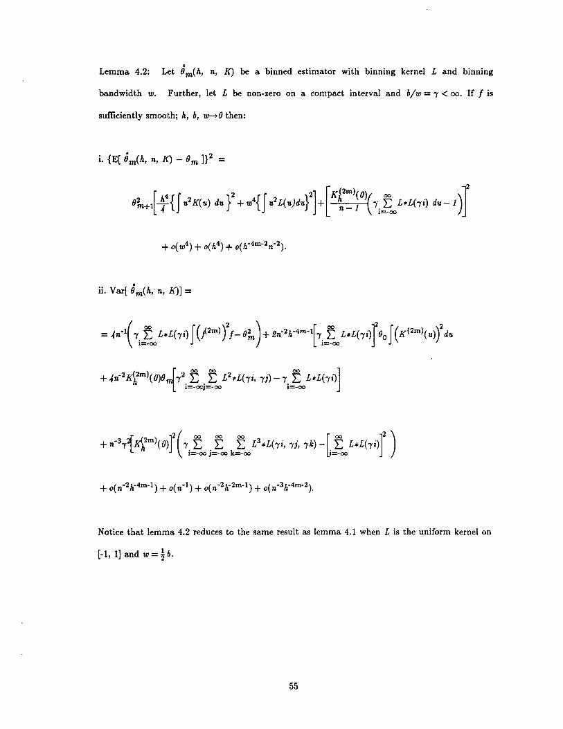
Lemma 4.2: Let 0m(h, n, K) be a binned estimator with binning kernel L and binning
bandwidth w. Further, let L be non-zero on a compact interval and h/w = I < 00. If f is
sufficiently smooth; h, h, w-O then:
. ' 21. {E[ (Jm(h, n, K) - (Jm]) =
•ii. Var[ (Jm(h, n, K)] =
Notice that lemma 4.2 reduces to the same result as lemma 4.1 when L is the uniform kernel on
[-1,1] and w=~h.
55
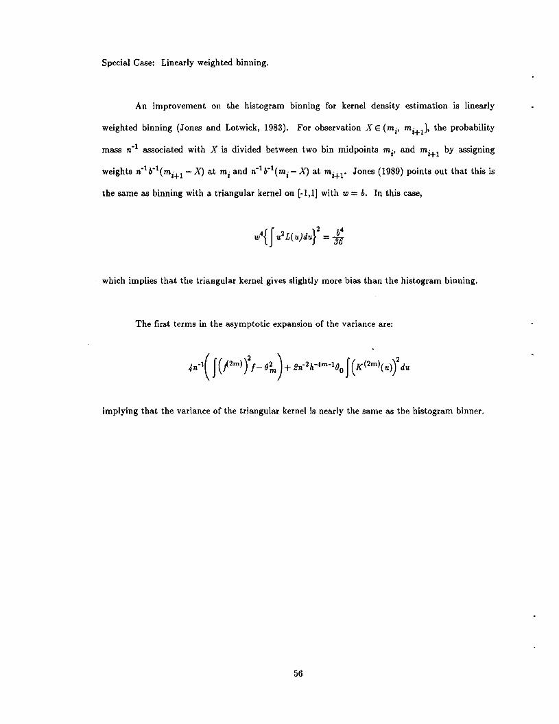
Special Case: Linearly weighted binning.
An improvement on the histogram binning for kernel density estimation is linearly
weighted binning (Jones and Lotwick, 1983). For observation X E (mi' mi+l]' the probability
mass n-1 associated with X is divided between two bin midpoints mi' and mi+! by assigning
weights n-1b-1(mi+! - X) at mi and n-1b-1(mi - X) at mi+!' Jones (1989) points out that this is
the same as binning with a triangular kernel on [-1,1] with w = b. In this case,
which implies that the triangular kernel gives slightly more bias than the histogram binning.
The first terms in the asymptotic expansion of the variance are:
implying that the variance of the triangular kernel is nearly the same as the histogram binner.
56
6. Proofs.
Proof of lemma 4.1:
Lemma 4.1.1: As 6......0,
fJ( x)dxfJ(y)dy = 62J( Cq)J( cr)+fif"( cq)J( cr) +/"( cr)J(Cq)) + o( 64).
I q I r
JJ(x)dxJJ(y)dyJJ(z)dz =Iq Ir Is
The proof of lemma 4.1.1 follows from a Taylor expansion of J(x) around the bin midpoints. 0
r..fO (h n K)]= f(_1)m{ E K(2m)(i6)[lq~r~inqnr]__1_K(2m)(o)}]Lt. m " L i = 0 h n( n - 1) (n - 1) h
57

Using lemma 4.1.1: E[Om(h, n, 10] =
Using Hall and Marron (1987):
[h2 {f 2 } b
2] 2 2=Om+ Om+12 uK(u)du +72 +o(b)+o(h).
ii. Variances:
Lemma 4.1.2: Let neal = n(n - 1) x ... x (n - a + 1). For q:f: r:f: s:f: t:
Var(n~) = E(n~) - E(n~)E(n~)
= 4n(3)p~ + 6n(2)p~ - 4n3p~ + (JOn2 - 6n)p~ - 4n(2)p~ - np~ + npq'
Cov(n~ n~) =E(n~ n~) - E( n~)E( n~)
= - 4n3p~p~+ (JOn2 - 6n)p~p~- 2n(2)P~Pr- 2n(2)pqP~_ npqPr'
Cov( n~, nqnr) = E( n~ nr) - E( n~)E( nqnr)
= 2n(3)P~Pr- 4n3p~Pr+ (JOn2 - 6n)p~Pr- 2n(2)P~Pr+ ni(2)PqPr
Var(nqnr) = E(n~ n~) -[E(nqnr)j
= n(3)P~Pr+ n(3)pqP~+ n(2)PqPr + (JOn2 - 6n)p~p~- 4n3p~p~
58

Cov( n~, nsnr) = E(n~nsnr) - E(n~)E(nsnr)
- / 3 2 (10 2 6) 2 2 (2)- - "n PqPrPs + n - n PqPrPs - n PqPrPs.
Cov( nqn,., nsnt) =E(nqnrnsnt) - E( nqnr)E(nsnt)
= - -/n3pqPrPsPt + (10n2
- 6n)pqPrPsPt-
Proof of lemma 4.1.2: (k )Ea.
All the identities are proved using E[n~al) x··· x nLak)] = n i=l 1 p~l x ... x ~k
and tedious algebra.
59
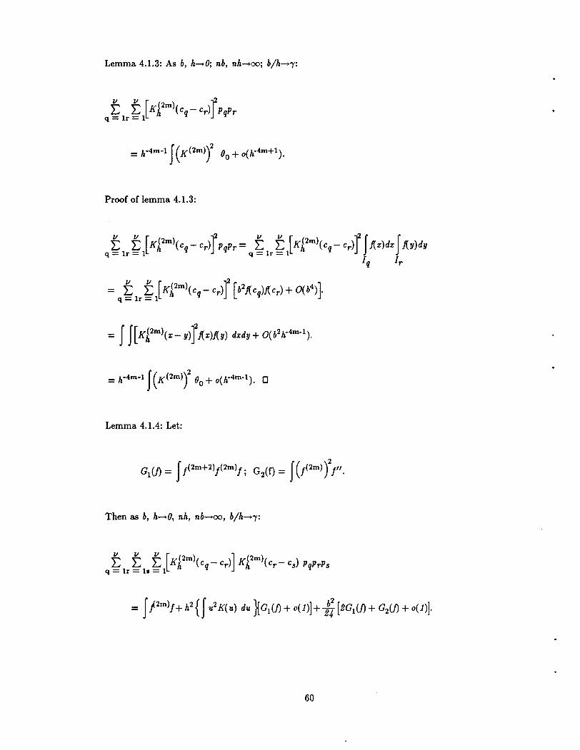
Lemma 4.1.3: As b, h...... Oj nb, nh......ooj b/h......"Y:
Proof of lemma 4.1.3:
Lemma 4.1.4: Let:
Then as b, h...... O, nh, nb......oo, b/h......"Y:
60
Proof of lemma 4.1.4:
= q t lr tIs t1Kk2m
)(Cq - Cr) Kk2m
)(c r - Cs) IJtx)dxIJty)dyIJt z)dz
Iq Ir Is
= IIIKk2m)(x- y) K~2m)(y_ z) Jtx)Jty)Jtz) dxdydz
+ ;;IIIKk2m)(x - y)Kk2m)(y - Z)(J"(X)Jty)Jtz) +J"(y)Jtx)Jt z) +J"(z)Jtx)Jty)) dxdydz
Using integration by parts:
Now return to proof of Lemma 4.1:
61
Combining terms and substuting using lemma 4.1.1 gives:
1 {(3) ~ ~ ~ (2m)( ) (2m)( )= 2 2 -In LJ LJ LJ Kh Cq - Cr Kh Cr - Cs PqPrPsn (n - 1) q =lr =Is =1
62
Using lemmas 4.1.2 and 4.1.3:
Proof of theorem 4.1 and theorem 4.2:
Immediate from lemma 4.1.
Proof of lemma 4.2:
•i. E[lJm(h, n, K)] =
63
For the first term:
(n-l)=-n- x
64

For the second term,
As 6-0:
Part i of lemma 4.2 follows directly. 0
For part ii of lemma 4.2:
65
Further,
=[J II12m)(x-y)J{X)J{y) dXdY+O(W)r
66
•
= t t t t b4 I12m)(Cq- Cr)I12m)(CS - Ct)(W-2I(Cq)I(Ct)L*L(-y [r- t]) Xq=lr=ls=lt=l
X L*L(-y [s - q]) + o(W·2))
00 00 min(i+II,II)min(HII,II)='}'2,E ,E L*L('}'i)L*L('}'i) E., E., b2I12m)(Cq-ct-ib)I12m)(cq+ib-ct)
l=-OOJ=-OO q=O 1 t=O J
X (I( Cq)1( Ct) + 0(1))
= '}'2112m)( 0), f .f L2*L('}'i, '}'i)( (} m + 0(1)).
l=-ooJ=-oo
67

Substituting and combining terms gives:
o
68
Chapter V: Asymptotics and Exact Calculations
1. Introduction:
A primary tool for studying smoothing estimators is asymptotics. The behavior of the
estimator is studied by examining its asymptotic behavior as the sample size, n, goes to infinity
and the bandwidth, h, goes to O. Since the bandwidth should not go to 0 too quickly, the
requirement that nh-oo is usually added.
An important question always raised by asymptotics is how large does n have to be
before the asymptotics approximate the true behavior well. The goal of the estimators discussed
in this research is generally minimizing their MSE. Usually, this is approached by minimizing
an asymptotic MSE. This chapter investigates how well the asymptotic MSE approximates the
true MSE.
2. Comparison of Asymptotic and Exact Risks.
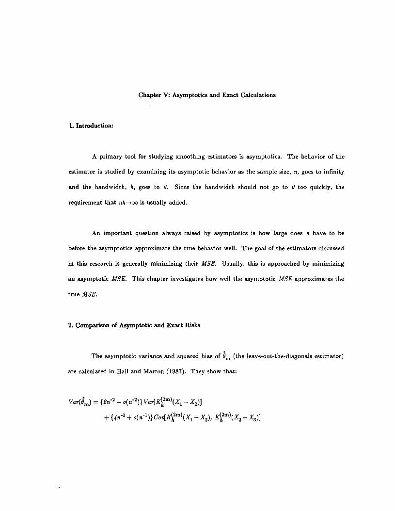
The asymptotic variance and squared bias of 8m (the leave-out-the-diagonals estimator)
are calculated in Hall and Marron (1987). They show that:
Var(0m) = {2n-2+ o(n-2)} Var{I12m)(Xl - X2)]
+ {4n-l + o(n-l )} COv(I12m)(Xl - X2), I12m)(X2 - X3 )]
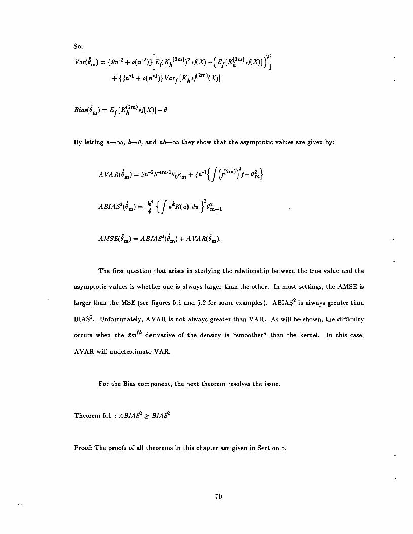
So,
Var(8m) = {2n-2+ o(n-2)}[EjKh(2m)2*.!tX) -(E/(R\2m)*.!tX)] YJ+ {.in-1 + o(n-1 )} Var/(Kh*pm)(X)]
By letting n-oo, h-O, and nh-oo they show that the asymptotic values are given by:
The first question that arises in studying the relationship between the true value and the
asymptotic values is whether one is always larger than the other. In most settings, the AMSE is
larger than the MSE (see figures 5.1 and 5.2 for some examples). ABIAS2 is always greater than
BIAS2• Unfortunately, AVAR is not always greater than VAR. As will be shown, the difficulty
occurs when the 2mth derivative of the density is "smoother" than the kernel. In this case,
AVAR will underestimate VAR.
For the Bias component, the next theorem resolves the issue.
Theorem 5.1 : ABIAS2 ~ BIAS2
Proof: The proofs of all theorems in this chapter are given in Section 5.
70
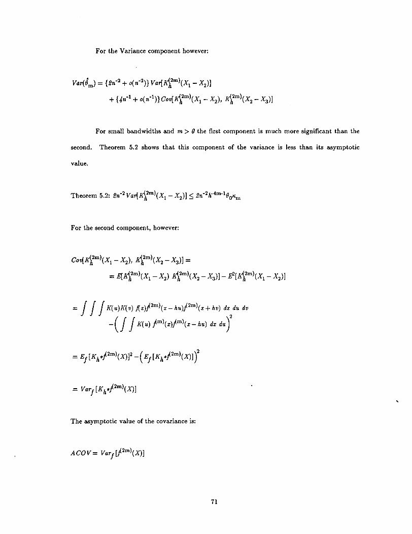
For the Variance component however:
Var(0m) = {2n-2+ o(n-2)} Var{R);m)(Xl - X2)]
+ {4n-l + o(n-l )} Cov(R);m) (Xl - X2), I12m)(X2- X3 )]
For small bandwidths and m > 0 the first component is much more significant than the
second. Theorem 5.2 shows that this component of the variance is less than its asymptotic
value.
For the second component, however:
COv(I12m)(Xl - X2), I12m)(X2- X3 )] =
= E1:I12m)(Xl - X2) I12m)(X2- X3 )] - ~[I12m)(Xl - X2)]
=JJJK(u)K(v) j(x)pm)(x_ hu)pm)(x+ hv) dx du dv
-(JJK(u) /m)(x)/m)(x_ hu) dx duy
The asymptotic value of the covariance is:
71
..
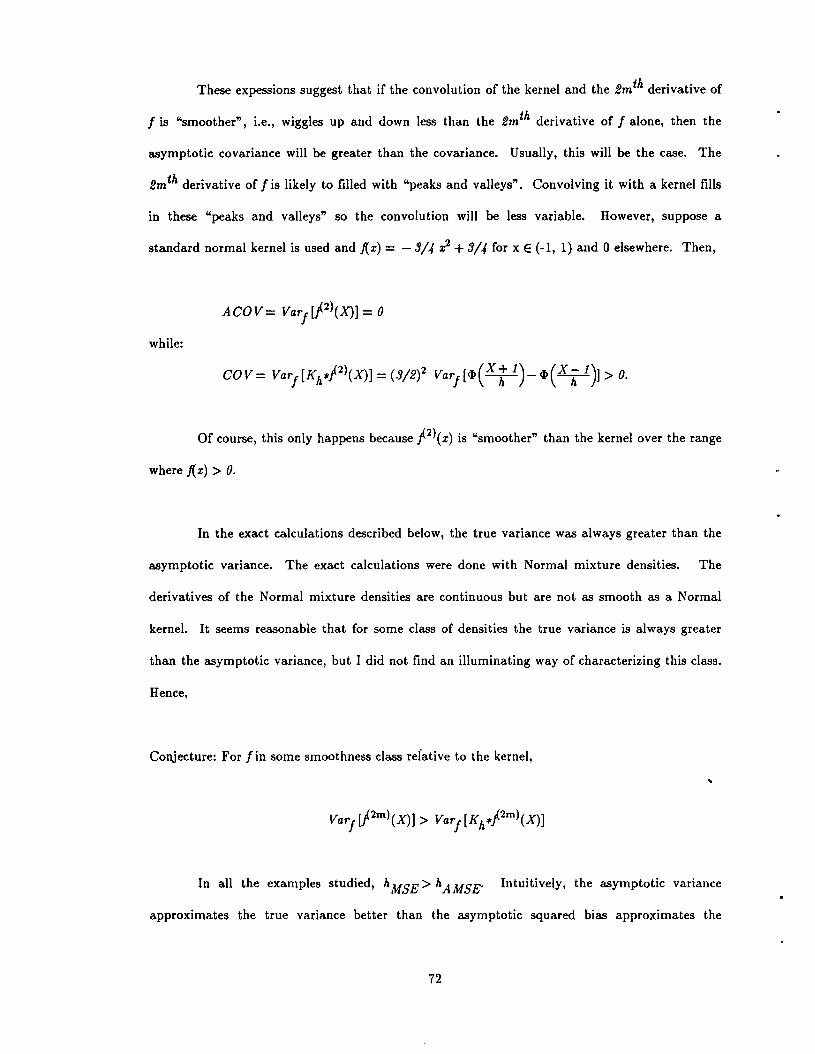
These expessions suggest that if the convolution of the kernel and the 2mth derivative of
f is "smoother", i.e., wiggles up and down less than the 2mth derivative of f alone, then the
asymptotic covariance will be greater than the covariance. Usually, this will be the case. The
2mth derivative of f is likely to filled with "peaks and valleys". Convolving it with a kernel fills
in these "peaks and valleys" so the convolution will be less variable. However, suppose a
standard normal kernel is used and J(x) = - 3/4 :t? + 3/4 for x E (-1, 1) and 0 elsewhere. Then,
while:
Of course, this only happens because f 2 }(x) is "smoother" than the kernel over the range
where J(x) > O.
In the exact calculations described below, the true variance was always greater than the
asymptotic variance. The exact calculations were done with Normal mixture densities. The
derivatives of the Normal mixture densities are continuous but are not as smooth as a Normal
kernel. It seems reasonable that for some class of densities the true variance is always greater
than the asymptotic variance, but I did not find an illuminating way of characterizing this class.
Hence,
Conjecture: For f in some smoothness class refative to the kernel,
..
In all the examples studied, hMSE > hAMSE' Intuitively, the asymptotic varIance
approximates the true variance better than the asymptotic squared bias approximates the
72
squared bias. The asymptotic squared bias is much greater than the squared bias. The
asymptotic variance is only slightly greater than the true variance. In trading-off asymptotic
variance and squared bias, hAMSE favors variance more than hMSE to avoid the inflated
asymptotic squared bias. Again, I do not have a general proof of this, so:
Conjecture: Under reasonable conditions: hMSE > hAMSE·
3. Exact MSE calculationS.
The asymptotics have several shortcomings. As with all asymptotics, it is difficult to
know how close the limiting values are to actual values using finite sample sizes and realistic
bandwidths. The asymptotics may require tremendously large sample sizes before they are a
reasonable approximation to truth. Secondly, the asymptotics contain constants that are
difficult to comprehend.
Another approach is to compute exact MSE's for a class of distributions that is
representative of a wide range of distributions. As will be shown below, if f is a mixture of
Gaussian densities (or even derivatives of Gaussian densities) and K is a Gaussian kernel, then it
•is possible to compute exact values for MSE(O h).m,
a. Lemmas and Notation:
Several lemmas are needed...
Lemma 5.1: For 0'1' 0'2 > 0, and r1, r2 = 0, 1, 2, ...
73
Lemma 5.2: For 0'1' 0'2 > 0, and r I , r2 = 0, 1, 2, ...
Lemma 5.3: For O'j > 0,
- 1 d -0' = "7, an J1. =0'
..
Lemma 5.4: For O'j > 0, and rj = 0, 1, 2, ...
where J1.j = J1.j - it
H,l..x) is the rth Hermite polynomial
OF( n) is the odd factorial of n
OF(x) = °if x is odd
74
The variance of 0m,h involves integrals like those in lemma 5.4. It is not very
enlightening to write the complete sum each time the integral appears in the variance. However,
the sum is straightforward to program, so the integral can be computed easily and exactly. Let
J TIn ",(rj)( ) d - I (- - -)'1'0" X - Ilj X = 1 r, Il, 0' •
j=1 J
where
ii = (0'1' 0'2' ••• , O'n)
Then:
Lemma 5.5:
where
Lemma 5.6:
r = (2m, 2m, 0)
i1n = (0, 0, Ilj -Il)
iit = (h, h, ~O'? + O'J).
where i1GI = (Iljt Iljt Ill)
iiGI = (~O'r + h2
, ~O'J + h2
, 0'/)
75
b. Theorems:
The lemmas above allow MSE(Om,h) to be computed for f a Gaussian mixture density.
For the theorems in this section suppose that f is a mixture of k Gaussian densities, Le.,
Theorem 5.3:
Theorem 5.4:
(n- 2)+4 n(n -1)
h -1 -1 I - -2 -2 * d fi d bwere JJijl O'ij' 11 r, JJijl' O'ijl' O'ij are as e me a ove.
Theorem 5.5:
•Of course, the MSE(Om,h) follows easily from the theorems.
76
4. Examples.
Figure 5.1 shows a typical example. The graph shows the asymptotic MSE and the true
variance, squared bias, and MSE of 82 for a wide range of bandwidths. The risks were
standardized by dividing them by (02)2. The Normal mixture density used is distribution #4
given in Appendix A. This distribution is not particularly spiky, and presents a relatively easy
estimation problem in this context. Several features are worth noting:
• For every bandwidth, AMSE > MSE.
• The asymptotic variance approximates the true variance much better than the asymptotic
squared bias approximates the true squared bias.
• hAMSEis fairly close to hMSE' Further, MSE(hAMSE) is not much greater than
MSE(hAMSE).
Figure 5.2 is identical to Figure 5.1 except Distribution #11 in Appendix A is used
instead. Distribution #11 is very spiky and presents a terrible estimation problem. Several
features distinguish this problem from the much easier problem posed by Distribution #4:
• hAMSE is not very close to hMSE" The intuition for this is that hAMSE is too heavily
impacted by trying to estimate the curvature in the spikes.
• MSE(hAMSE) is much greater than MSE(hAMSE)·
• The asymptotic squared bias is a terrible approximation to the true squared bias.
77
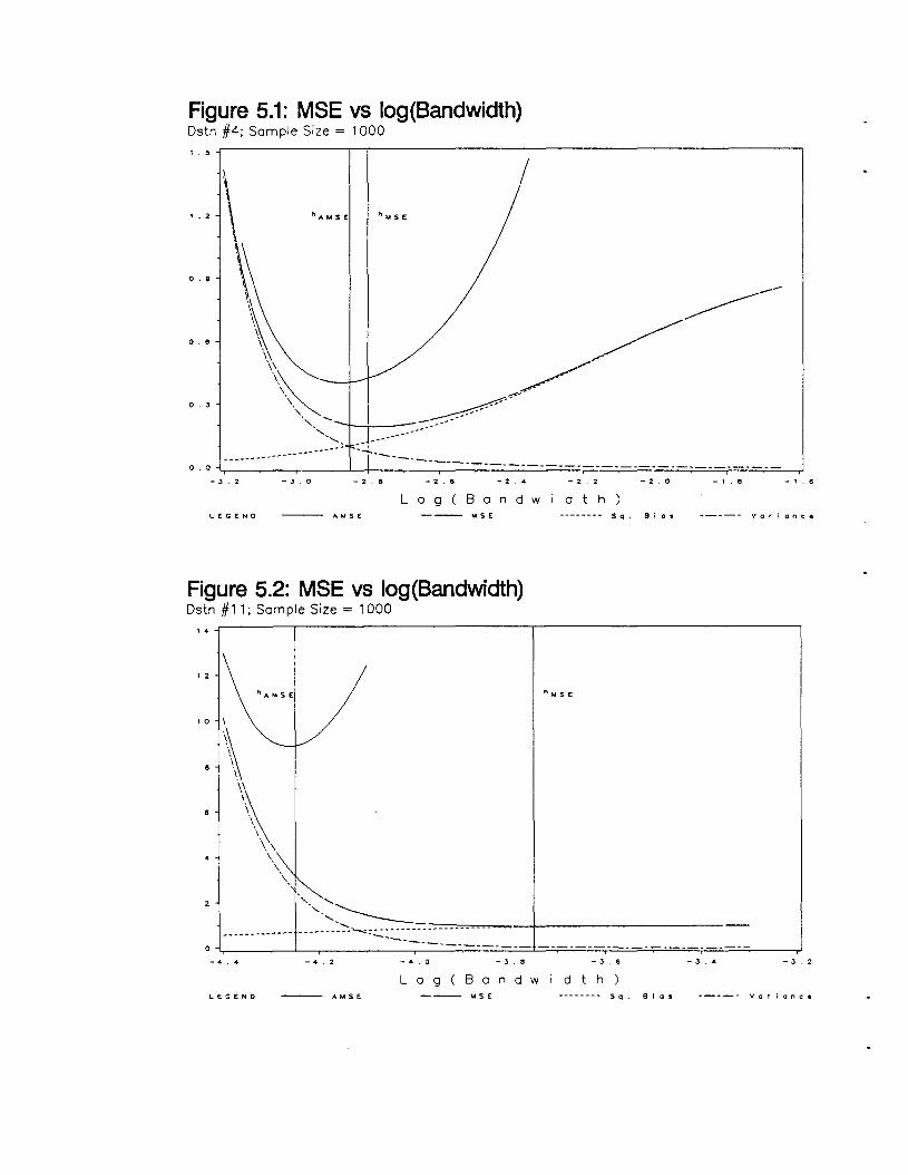
Figure 5.1: MSE vs log(Bandwidth)Dstn #4; Sample Size = 10001 . ~ ..r--------.-.,-----------------------------,
1 .2
0.9
0.8
0.3
...... - ..
- 1 . 5- 1 • e-2.0- 2 . 2-2.4- 2 . IS- 2 . S- 3 0
._-------o . 0 -t.,-------r---.L-+--~-___r---~------=..:--;=.-=-:.:-~-=-:.:-=..:.;--=-=-::..:-==-=--=;.-=-:.:-c.;:-=.;-;..:-=--=;:.-=-:.;-:.=-=--=---,J
- J . 2
Log ( Ban d wid t h )'- E: C END AMSE --- MS' -------- Sq. B i as Variance
Figure 5.2: MSE vs log(Bandwidth)Dstn #11; Sample Size = 1000
1 •
12
10
o
h AMSELJ h M S E
I
\II
'\\~\
\
'~,",,~
--------- ---- ------ -_':":.~:.. -_ ... _.. ------------_ .. ----------------- - - - - - - - - - - -- 4 . 4 - .... 2 - .... 0 - J . S - 3 . 6 - J .... - J . 2
Log ( Ban d wid t h )LECEND --- AMSE --- MS' -------- Sq. 8 I as Variance
5. Proofs.
Proof of Theorem 5.1:
From Hall and Marron (1987),
Using the integral form of Taylor's remainder theorem:
So by a change of variables,
Integrating by parts,
So by Cauchy-Schwarz:
IBias I ::::; h2 8mJu2K(u) du = IABias I·
Proof of Theorem 5.2:
80
So by a direct application of Cauchy-Schwarz:
Proof of Lemma 5.1: This is Theorem 4 in Aldershof, et. al. (1990).
Proof of Lemma 5.2: This is Corollary 4.4 in Aldershof, et. al. (1990).
Proof of Lemma 5.3: This is Theorem 3 in Aldershof, et. al. (1990).
Proof of Lemma 5.4: This is Theorem 5.1 in Aldershof, et. al. (1990).
Proof of Lemma 5.5:
From Hall and Marron (1987),
Using Lemma 5.2:
81
Proof of Lemma 5.6:
From Hall and Marron (1987),
=JJJh-4m~2m)(U)~2m)(V)j(x+hu)j(x)j(x_hv) dx du dv.
Using Lemma 5.1:
Proof of Theorem 5.3:
From Hall and Marron (1987),
82
Using Lemma 5.1:
Using Lemma 5.2:
Proof of Theorem 5.4:
The proof follows easily from the lemmas. First,
The result then fQllows from substitution and counting terms.
Proof of Theorem 5.5: Follows directly from Lemma 5.2.
83
Chapter VI: Estimability of 8m and m
1. Introduction.
The object of this section is to answer the question "How much more difficult is it to
estimate Bm +! than Bm ?". Intuitively, it seems that Bm should become increasingly difficult to
estimate as m grows larger. In other words, the larger m is, the larger the sample size that
should be required to estimate Bm with some fixed accuracy. In general, integration smooths a
function and differentiation makes it more jagged. The more jagged a function is, the more
data that is required to resolve its features. The purpose of this section is to clarify this
intuition by providing it with some mathematical basis and quantification.
2. Asymptotics.
a. Assumptions.
In this section assume that the kernel K is a probability density function. We also need
to assume some smoothness on the density f. Specifically, f has smoothness of order p when a
constant M> 0 exists so that for all x, y and 0 < cr ~ 1 :
where p =/+ cr. Assume that p ~ m + 2.
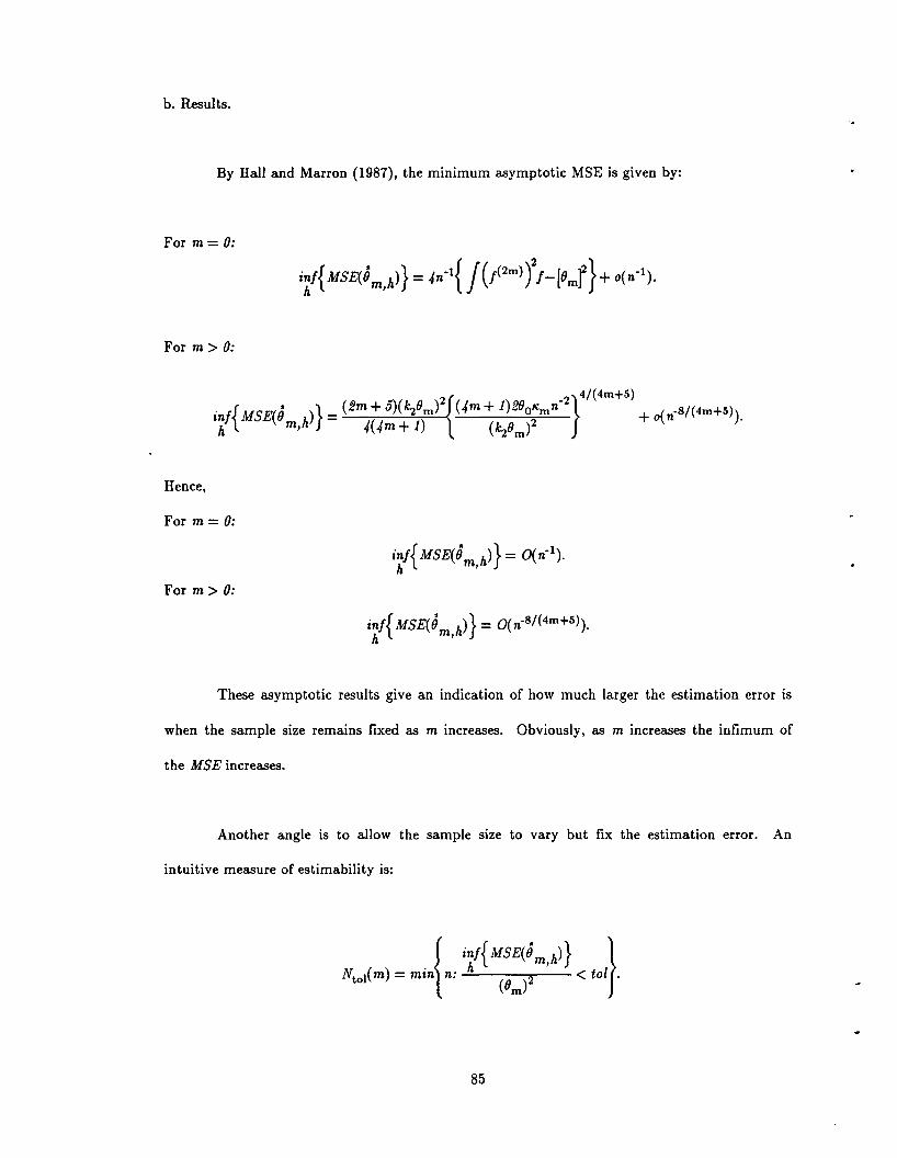
b. Results.
By Hall and Marron (1987), the minimum asymptotic MSE is given by:
For m = 0:
For m> 0:
Hence,
For m = 0:
For m> 0:
inf{MSE(B )} = O(n-8/(4m+5)).h m,h
These asymptotic results give an indication of how much larger the estimation error is
when the sample size remains fixed as m increases. Obviously, as m increases the infimum of
the MSE increases.
Another angle is to allow the sample size to vary but fix the estimation error. An
intuitive measure of estimability is:
85
In other words, Ntol is the smallest sample size necessary so that, for some bandwidth, the
standardized MSE is less than tol (tol stands for "tolerance"). Using the above equations it is
easy to see that (suppose here that m> 0):
Ntol(m) "" C(m, f)(tol)-(4m+5)/8 .
where C( m, f) is a constant depending on m and the density f. The asymptotic expression for
Ntol provides one answer to the question "How much more difficult is it to estimate 8m+! than
The difficulty with this answer is that the constant terms are complicated. It does make clear,
however, that if tol is very small (Le., very accurate estimation is required) it is much harder to
estimate 8m+1 than 8m ,
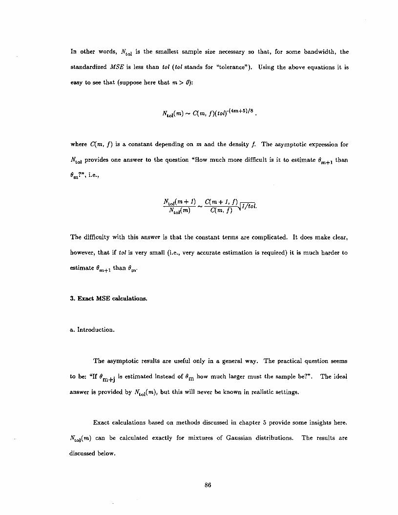
3. Exact MSE calculations.
a. Introduction.
The asymptotic results are useful only in a general way. The practical question seems
to be: "If 8m+j is estimated instead of 8m how much larger must the sample be?". The ideal
answer is provided by Ntol(m), but this will never be known in realistic settings.
Exact calculations based on methods discussed in chapter 5 provide some insights here.
Ntol(m) can be calculated exactly for mixtures of Gaussian distributions. The results are
discussed below.
86
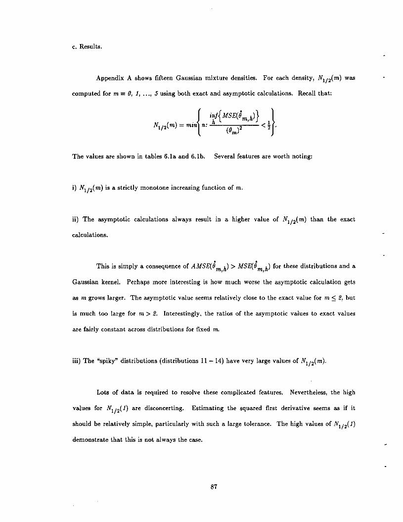
c. Results.
Appendix A shows fifteen Gaussian mixture densities. For each density, N1/im) was
computed for m = 0, 1, ..., 5 using both exact and asymptotic calculations. Recall that:
The values are shown in tables 6.1a and 6.1b. Several features are worth noting:
i) N1/ 2( m) is a strictly monotone increasing function of m.
ii) The asymptotic calculations always result in a higher value of N1/ 2( m) than the exact
calculations.
• •This is simply a consequence of AMSE(0m h) > MSE(0m h) for these distributions and a, ,
Gaussian kernel. Perhaps more interesting is how much worse the asymptotic calculation gets
as m grows larger. The asymptotic value seems relatively close to the exact value for m ~ 2, but
is much too large for m> 2. Interestingly, the ratios of the asymptotic values to exact values
are fairly constant across distributions for fixed m.
iii) The "spiky" distributions (distributions 11-14) have very large values of N1/ 2(m).
Lots of data is required to resolve these complicated features. Nevertheless, the high
values for N1/ 2( 1) are disconcerting. Estimating the squared first derivative seems as if it
should be relatively simple, particularly with such a large tolerance. The high values of N1/ 2(1)
demonstrate that this is not always the case.
87
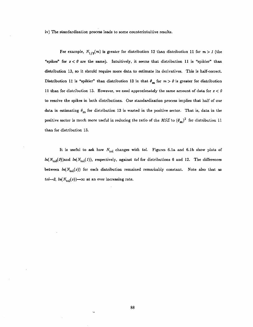
iv) The standardization process leads to some counterintuitive results.
For example, N1/ 2( m) is greater for distribution 13 than distribution 11 for m> 1 (the
"spikes" for x < 0 are the same). Intuitively, it seems that distribution 11 is "spikier" than
distribution 13, so it should require more data to estimate its derivatives. This is half-correct.
Distribution 11 is "spikier" than distribution 13 in that Om for m> 0 is greater for distribution
11 than for distribution 13. However, we need approximately the same amount of data for x < 0
to resolve the spikes in both distributions. Our standardization process implies that half of our
data in estimating Om for distribution 13 is wasted in the positive sector. That is, data in the
positive sector is much more useful in reducing the ratio of the MSE to (Om)2 for distribution 11
than for distribution 13.
It is useful to ask how Nto1 changes with tol. Figures 6.1a and 6.1b show plots of
In(Nto1(O»and In(Nto1(1», respectively, against tol for distributions 6 and 12. The differences
between In(Nto1(x» for each distribution remained remarkably constant. Note also that as
tol-O, In(Nto1(x»-oo at an ever increasing rate.
88
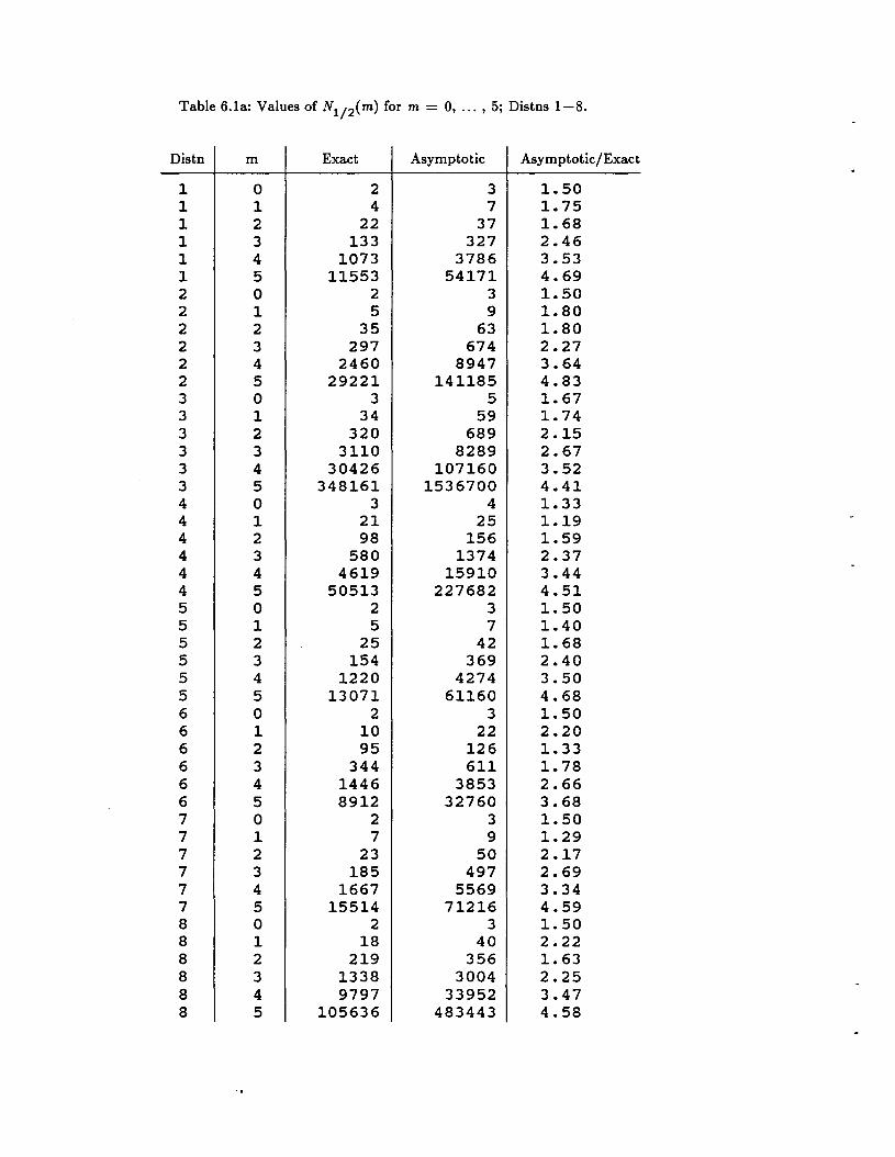
Table 6.1a: Values of N1/ 2 (m) for m = 0, ... , 5; Distns 1-8.
Distn m Exact Asymptotic Asymptotic/Exact
1 0 2 3 1.501 1 4 7 1. 751 2 22 37 1.681 3 133 327 2.461 4 1073 3786 3.531 5 11553 54171 4.692 0 2 3 1.502 1 5 9 1.802 2 35 63 1.802 3 297 674 2.272 4 2460 8947 3.642 5 29221 141185 4.833 0 3 5 1.673 1 34 59 1.743 2 320 689 2.153 3 3110 8289 2.673 4 30426 107160 3.523 5 348161 1536700 4.414 0 3 4 1.334 1 21 25 1.194 2 98 156 1.594 3 580 1374 2.374 4 4619 15910 3.444 5 50513 227682 4.515 0 2 3 1.505 1 5 7 1.405 2 25 42 1. 685 3 154 369 2.405 4 1220 4274 3.505 5 13071 61160 4.686 0 2 3 1. 506 1 10 22 2.206 2 95 126 1. 336 3 344 611 1.786 4 1446 3853 2.666 5 8912 32760 3.687 0 2 3 1.507 1 7 9 1.297 2 23 50 2.177 3 185 497 2.697 4 1667 5569 3.347 5 15514 71216 4.598 0 2 3 1. 508 1 18 40 2.228 2 219 356 1. 638 3 1338 3004 2.258 4 9797 33952 3.478 5 105636 483443 4.58
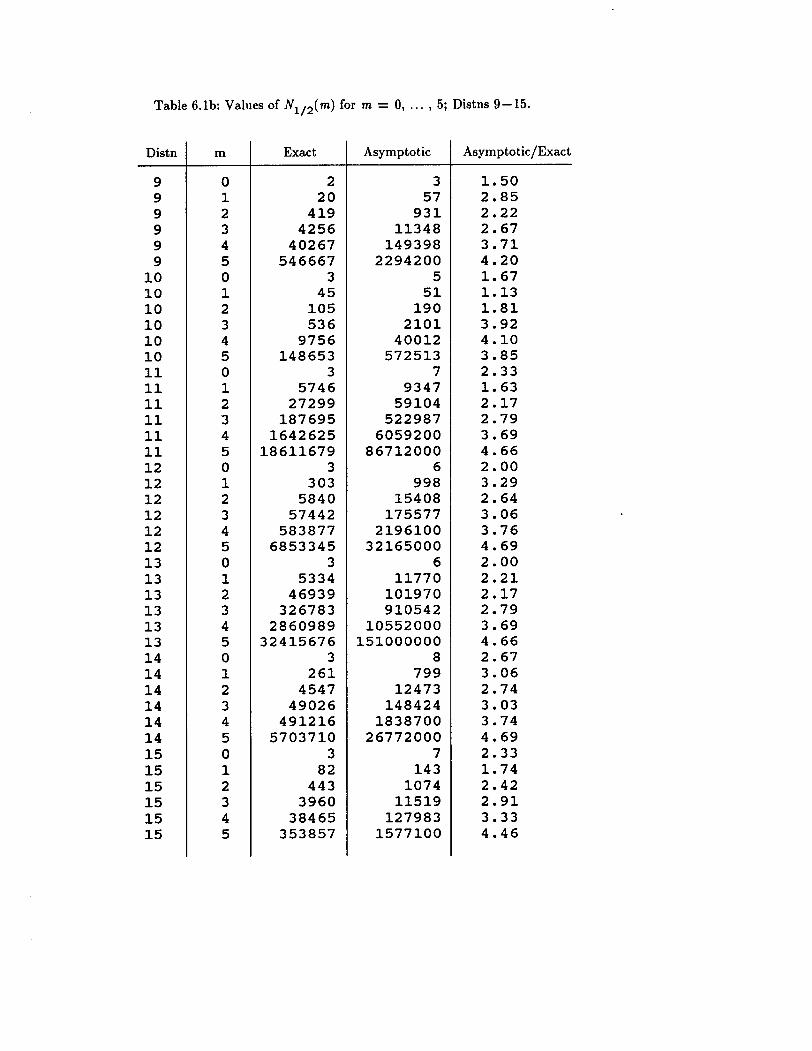
Table 6.1b: Values of N1/ 2 (m) for m = 0, ... , 5; Distns 9-15.
Distn m Exact Asymptotic Asymptotic/Exact
9 0 2 3 1.509 1 20 57 2.859 2 419 931 2.229 3 4256 11348 2.679 4 40267 149398 3.719 5 546667 2294200 4.20
10 0 3 5 1. 6710 1 45 51 1.1310 2 105 190 1.8110 3 536 2101 3.9210 4 9756 40012 4.1010 5 148653 572513 3.8511 0 3 7 2.3311 1 5746 9347 1. 6311 2 27299 59104 2.1711 3 187695 522987 2.7911 4 1642625 6059200 3.6911 5 18611679 86712000 4.6612 0 3 6 2.0012 1 303 998 3.2912 2 5840 15408 2.6412 3 57442 175577 3.0612 4 583877 2196100 3.7612 5 6853345 32165000 4.6913 0 3 6 2.0013 1 5334 11770 2.2113 2 46939 101970 2.1713 3 326783 910542 2.7913 4 2860989 10552000 3.6913 5 32415676 151000000 4.6614 0 3 8 2.6714 1 261 799 3.0614 2 4547 12473 2.7414 3 49026 148424 3.0314 4 491216 1838700 3.7414 5 5703710 26772000 4.6915 0 3 7 2.3315 1 82 143 1.7415 2 443 1074 2.4215 3 3960 11519 2.9115 4 38465 127983 3.3315 5 353857 1577100 4.46
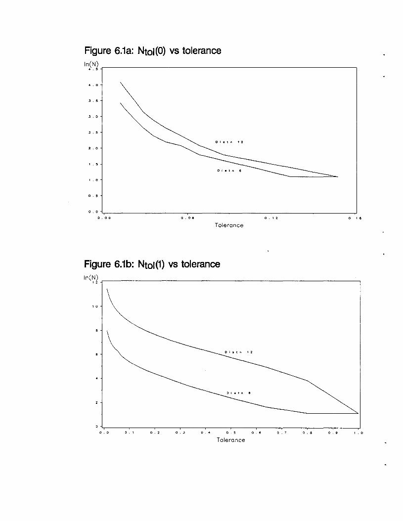
o . 1 8o . 1 20.06
, .0
2 . ~
1 . ~
O. 0 '-r------~----_,..._-----~----_,..._-----~----___,_Jo. 00
3.0
2.0
3.~
o . ~
'.0
Figure 6.1a: Ntol(O) vs toleranceIn$N~ ...- -----,
Tolerance
Figure 6.1b: Ntol(1) vs tolerance
'n(~l...----------------------------------,
, 0
0'r-----,----r------r------,---,--------r----,.----...,-------,--------r'0.0 o . , O. 2 o . 3 0.' o . ~ o . 6 o . 7 o . 8 o . 9 1 .0
Tolerance
Chapter Vll: The "One-Step" Estimator
1. Introduction.
Hall and Marron (1987) provide the asymptotic' MSE optimal bandwidth for estimating
8m using the "leave-out-the-diagonals" estimator for m;::: 1. This bandwidth is given below in
theorem 7.1. The difficulty is that the bandwidth is a function of 80 and 8m+!. both of which
are presumably unknown. It seems that for practical estimation problems, this "optimal"
bandwidth is of little help.
This chapter discusses a "one-step" estimator in which a kernel estimator of 8m+! is
used to estimate the optimal bandwidth for 8m, Of course, the estimator of 8m+! also requires a
bandwidth so it is apparently no improvement over the "no-step" estimator. It will be shown
that the "one-step" estimator can be less sensitive to this choice of bandwidth. That is,
deviations from the optimal bandwidth do not cause large deviations in its MSE compared to
the "no-step" estimator. The cost of this is that with optimal choices of bandwidth the "one-
step" estimator has higher MSE than the "no-step" estimator.
The "one-step" estimator provides a compelling reason to calculate a "leave-in-the
..diagonals" estimator. If the kernel estimate of 8m+! is negative, the "one-step" estimator is a
kernel estimator with a bandwidth that is a fractional root of a negative number. To avoid this,
the kernel estimator for 8m+! used below is the "leave-in-the diagonals" estimator since it is
always positive. The kernel estimator for 8m below is the "leave-out-the-diagonals" estimator.
The "leave-in-the diagonals" estimator is discussed in chapter VIII.
Since (Jo is much easier to estimate than (Jm for m> 0, in this chapter (Jo will be
considered known. A complete demonstration and explanation of this is found in chapter VI.
Hall and Marron (1987) show that the bandwidth selection problem for (Jo is also much easier
than for (Jm' For moderately smooth f, any sequence of bandwidths, {hn } such that
n-1/(4m+I) < hn < n-1/ 4 ,for m the order of the kernel, provides the asymptotically optimal MSE
convergence rate for 00' Since there is no unknown functional needed in this sequence, (Jo has no
"one-step" estimator. All the results in this chapter are valid only for estimating (Jm for m ~ 1.
2. Assumptions and Notation.
Let:
where K is a convolution density function. Some technical problems are avoided by assuming
that Om is bounded away from O. This follows from any number of conditions including f
having compact support, 0- being bounded a.s., Jhaving compact support, and many others. In
practical problems, Om is usually very large so the assumption is not too important for practical
results.
A "leave-out-the-diagonals" estimator will be denoted:
..
Several functionals of the kernel are abbreviated. They are:
93
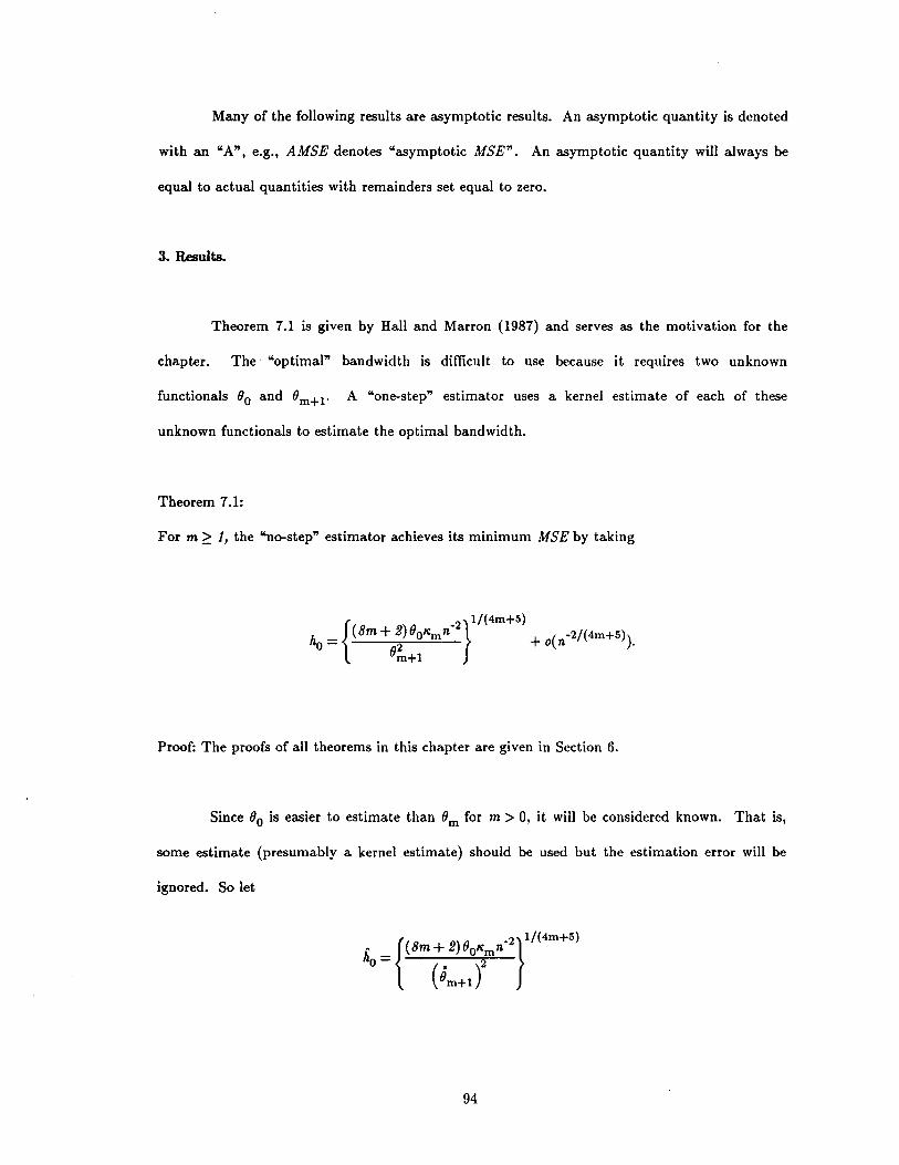
Many of the following results are asymptotic results. An asymptotic quantity is denoted
with an "A", e.g., AMSE denotes "asymptotic MSE". An asymptotic quantity will always be
equal to actual quantities with remainders set equal to zero.
3. Results.
Theorem 7.1 is given by Hall and Marron (1987) and serves as the motivation for the
chapter. The· "optimal" bandwidth is difficult to use because it requires two unknown
functionals 80 and 8m+1. A "one-step" estimator uses a kernel estimate of each of these
unknown functionals to estimate the optimal bandwidth.
Theorem 7.1:
For m ~ 1, the "no-step" estimator achieves its minimum MSE by taking
{
2}1/(4m+5)h _ (8m+ 2)80Km n" ( -2/(4m+S))0- 2 +0 n .
8m +!
Proof: The proofs of all theorems in this chapter are given in Section 6.
Since 80 is easier to estimate than 8m for m> 0, it will be considered known. That is,
some estimate (presumably a kernel estimate) should be used but the estimation error will be
ignored. So let
94
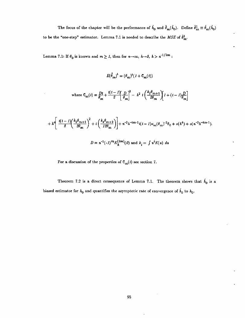
The focus of the chapter will be the performance of ho and 0m(ho). Define O:n == 0m(ho)
to be the "one-step" estimator. Lemma 7.1 is needed to describe the MSE of O:n.
Lemma 7.1: If°0 is known and m ~ 1, then for n-+oo, h-+O, h> n-1/ 2m :
For a discussion of the properties of em(t) see section 7.
Theorem 7.2 is a direct consequence of Lemma 7.1. The theorem shows that ho is a
biased estimator for ho and quantifies the asymptotic rate of convergence of ho to ho.
95
Theorem 7.2: If 00 is known, then for n-oo, h-O, h> n-1/2m :
Lemmas 7.2 and 7.3 describe the squared bias and variance of O:n. Of course, these are
necessary for describing the MSE(O:n). Notice that the bias looks similar to the bias for the
known optimal bandwidth except for the term involving the e-function. The variance is also
similar except a term that looks like bias is added on and it contains an additional e-function.
Lemma 7.2: If 00 is known, then for n-oo, h-O, h> n-1/2m :
Lemma 7.3: If 00 is known, then for n-oo, h-O, h> n-1/2m :
Theorem 7.3 describes the MSE for O:n. Theorem 7.3 is the main result of the chapter.
Theorem 7.3: If 00 is known, then for n-oo, h-O, h> n-1/2m :
96
Note:
Theorem 7.3 provides the motivation for using the one-step estimator. As long as h is
chosen so that MSE(Om+t(h)) is relatively small, MSE(O~) is equal to the optimal value for
AMSE(Om) plus a small, positive remainder. Note that the "one-step" MSE is larger than the
optimal MSE for a kernel estimator of Om on two counts. First, since the "one-step" bandwidth
estimates an asymptotic MSE optimal bandwidth (rather than the actual MSE optimal
bandwidth), the best that can be hoped for is that the "one-step" MSE is close to the infimum
of the asymptotic MSE. By Chapter V, this is greater than the infimum of the MSE. Second,
the remainder term is positive and, in fact, unbounded for terrible choices of h.
For optimal bandwidths, the one-step estimator has higher MSE than the no-step
estimator. However, notice that the remainder term resembles the squared bias of the no-step
estimator at its asymptotic MSE optimal bandwidth, Le.,
Remainder:
Squared Bias: ], 4 Ju2K( u) du [0 f
'00 4 m+t
For a reasonable choice of h (and large n) we should have MSE(Om+t(h)) < [Om+tf. An
indication of how large n must be is given by Chapter VI. Hence, in MSE, the "one-step"
estimator resembles the "no-step" estimator at its asymptotically optimal bandwidth plus some
added bias.
97
Corollary 7.3.1: For any fixed bandwidth h:
-8
MSE(O:n(h)) = O(n4m+5).
Corollary 7.3.1 is a consistency result. For a fixed bandwidth, increasing the sample
size causes the MSE to go to zero. In contrast, for a fixed bandwidth the "no-step" estimator is
not consistent since its bias is unaffected by sample size.
Corollary 7.3.1 seems startling. A consistent estimator is nearly always preferred over a
non-consistent estimator. This corollary seems to imply that the "one-step" estimator is a much
better than the "no-step" estimator. Some intuition may help clarify the corollary..Notice that
the "one-step" bandwidth is given by:
• (. )-2/(4m+5)ho = constant x nOm +1
So as n--oo, lio = lio(n) =6\ n-2/(4m+5»). The "one-step" estimator is consistent because of this
explicit tie between the bandwidth and the sample size. The "no-step" estimator is similarly
consistent for any sequence of bandwidths {hn} such that hn = 6\ n-2/(4m+5»).
Corollary 7.3.2 provides some guidance for bandwidth selection.
Corollary 7.3.2: If 00 is known, then for n--oo and h--O, the AMSE(O:U) is minimized by
which is also the bandwidth that minimizes AMSE(Om+I)'
98
The most interesting aspect of Corollary 7.3.2 is that AMSE(O:n) is minimized by the
same bandwidth that minimizes AMSE(Om+l)- This is a nice optimality property. The
optimal AMSE bandwidth for Om+! is also optimal for estimating the bandwidth for Om-
Corollary 7.3.3 is best motivated by looking at Figures 7.1a and 7.1b. These figures
show plots of standardized AMSE(OI(h)) and AMSE(0t(h)) for Normal mixture distribution #2
in Appendix A. The difference between the optimal bandwidths along the X-axis is not
meaningful. In 0I(h), h is used in the kernel estimate of 0I. In 0t(h), h is used in the kernel
estimate of 0m+!- The difference along the Y-axis between the minimum AMSE's is important.
This difference can be viewed as the cost of using the optimal "one-step" estimator instead of
the optimal "no-step" estimator. Corollary 7.3.3 shows that the optimal "one-step" estimator
has AMSE which converges to the AMSE of the optimal "no-step" estimator and quantifies the
rate.
Corollary 7.3.3: For known 0o, if ho' hI are chosen as in theorems 7.1 and 7.3 respectively, then
as n-oo and h-O:
Notice that the rate given in corollary 7.3.3 is:
See Figures 7.3a and 7.3b for a depiction of Corollary 7.3.3.
99
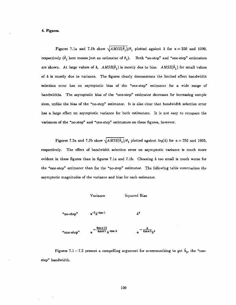
4. Figures.
Figures 7.1a and 7.1b show ~AMSE(01)/01 plotted against h for n = 250 and 1000,
respectively (01 here means just an estimator of 01), Both "no-step" and "one-step" estimators
are shown. At large values of h, AMSE(01) is mostly due to bias. AMSE(01) for small values
of h is mostly due to variance. The figures clearly demonstrate the limited effect bandwidth
selection error has on asymptotic bias of the "one-step" estimator for a wide range of
bandwidths. The asymptotic bias of the "one-step" estimator decreases for increasing sample
sizes, unlike the bias of the "no-step" estimator. It is also clear that bandwidth selection error
has a large effect on asymptotic variance for both estimators. It is not easy to compare the
variances of the "no-step" and "one-step" estimators on these figures, however.
Figures 7.2a and 7.2b show ~AMSE(01)/01 plotted against /og(h) for n = 250 and 1000,
respectively. The effect of bandwidth selection error on asymptotic variance is much more
evident in these figures than in figures 7.1a and 7.1b. Choosing h too small is much worse for
the "one-step" estimator than for the "no-step" estimator. The following table summarizes the
asymptotic magnitudes of the variance and bias for each estimator.
"no-step"
"one-step"
Variance Squared Bias
Figures 7.1 - 7.2 present a compelling argument for oversmoothing to get ho' the "one-
step" bandwidth.
100
1000,
~AMSE(Ol)Figures 7.3a and 7.3b show ( ~ .) plotted
(Jl x min AMSE«(J~)against h for n = 250 and
respectively where O~ is the "no-step" estimator. The purpose of these pictures is to show that
the relative difference between the minimum AMSE's for the "no-step" and "one-step"
estimators decreases with increasing sample size. The figures illustrate Corollary 3.3.
Figures 7.4a and 7.4b show em(t) for m = 2, f a standard Normal density, K a Gaussian
kernel, and several values of n, t, and h. The values of t chosen were important in some of the
theorems above. Notice that as the sample size increases and the bandwidths decrease em(t)
approaches o.
5. Conclusions.
The "one-step" estimator has several appealing properties. First, its MSE decreases
with sample size for any bandwidth. In other words, no matter how terrible a bandwidth is
selected, gathering more data improves the estimator. In contrast, a terrible bandwidth
selection for a "no-step" estimator may overwhelm the estimator with bias that will never go
away, regardless of the sample size. Second, even with optimal choices of bandwidths the "one-
step" is not much worse than the no-step. Finally, the "one-step" estimator is much less
affected by an oversmoothing bandwidth than the "no-step" estimator.
The disadvantage of the "one-step" estimator is that it is highly affected by
undersmoothing bandwidths. The "one-step" also involves more computing time.
A reasonable approach to choosing the "one-step" bandwidth is to use an oversmoothing
101

bandwidth based on minimum values of JU(m))2 as given in Terrell (1990) or Terrell & Scott
(1985). These bandwidths are the largest bandwidths that could possibly be optimal based on
some measure of sample variability. This approach seems a bit extreme so bandwidths based
on J(c/J(m))2 for c/J a Gaussian p.d.f. may be better and will still likely be oversmoothing.
The over-smoothing approach illustrates the real advantage of the "one-step" estimator.
It is easy to choose an oversmoothing bandwidth. If the oversmoothing bandwidth performs
almost as well as the optimal bandwidth then the bandwidth selection problem disappears.
102
Figure 7.1a: MSE vs BandwidthDstn #2; Sample size = 250
v'MSE/e~ --,1 . 0
o.~
0.8
0.7
1 -. t • p
0.8
o.~
o .•
o . 3 l ======:=S::;:::;:;;>'::::'-'I-~o . 2
O.
0.0 0.1 0.2 0.3 0.4 0.5 0.8 0.7 0.8 0.9 1.0 1.1 1.2 1.3
Ban d wid t h.. . 5
Figure 7.1b: MSE vs BandwidthDstn #2; Sample size = 1000
v'MS~/~.,r------------------------------,
o . ~
o 8
O-step
o . 7
o . 6
o . 5
o .•
o . 3
o . 2
o . 1
o . 0 -",...--.----r--r-:.---.--...----,.----r---.,...----,---r--.----r---r----r---.,.Jo 0 o. 0.2 0.3 0.4 0.5 0.8 0.7 0.8 0.9 1.0 1.1
Ban d wid t h. 3 t -4 . 5

0.9
O-step
o . ,
o . 7
0.&
0.8
Figure 7.2a: MSE vs log(Bandwidth)Dstn #2; Sample size = 250
v'MSE/e~ --,1 .0
o .•
o . 3 l ==========~====r=~;;;'-""::::::::::'I----~o . 2
O. 1
- 0 . 2-0.5-0.8- 1 • 1- 1 .4- t • 7
o . 0 "1,----~--,r-~-~--r----.-:.._r-~-~~_r_-~-~_r-~---__,J
-2.0
log ( Ban d w d t h )
Figure 7.2b: MSE vs log(Bandwidth)Dstn #2; Sample size = 1000
v'MS~/~~ ---,
o . 9
o . 8
o . 7
o .•
O-step
o . ,
o .•
o . 3
o . 2
o . 1
- 0 •- 0 . 7- , .0- , . 3- 1 .6- 1 • g- 2 . 2
o . 0 "1,--~~--r-~--_r-------.--""":""_--r-~--:'-'---~--.----__,J
- 2 . 5
log ( Ban d wid t h )
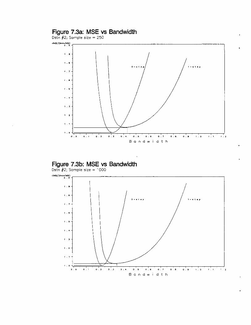
Figure 7.3a: MSE vs BandwidthDstn #2; Sample size = 250
"I\,oSE/(em"2'~~J""""-------------------------------------------,
1 • Q
1 • e
1 . 7
1 • e
1 . 5
1 .•
1 . 3
. 2
t - • t e p
1 . 0 -l.,====;r====r====;:::::::.~__,.....!~-.,..._~-__r-~__,---.,..._~-__r-~__,---.,..._~-_,J0.0 o . 1 o . 2 o . 3 o .4 O. 5 o . 8 o . 7 o.e O. 1 .0 . 2
8 and wid t h
Figure 7.3b: MSE vs BandwidthDstn #2; Sample size = 1000
.,I"SE/(em;n;"'5~J""""--------------------------------------------,
.Q
o 0 O. o . 2 0.3 o .• o . 5 o . o . 7 0.8 O. 1 .0 . 2
8 and wid t h
6. Proofs
Proof of Theorem 7.1: This is Theorem 2 in Hall and Marron (1987).
A lemma is necessary before proving lemma 7.1.
Let:
Proof of lemma 7.1.1:
.By assumption, (}m' and hence p, is bounded below by some positive f.
So,
Since the "diagonals" are simply a constant shift, the skewness of Om is the same as Om' To
ease some calculations we will calculate the third central m~ment of Om instead of Om'
where J.l =E(Om) now.
106
..
So let:
,Also, let ':Pn(Y) = (n~'y)!
By Hall and Marron (1987),
107
jJ =Om + 0(1).
Combining these with similar calculations show:
E3 = jJ h-4m-1( J/2)(J(~2m»)2)+ o(h-4m-1).
E4 = J(t<2m) )3/+ 0(1).
Es = h-6m-1( J/2)(J(~2m)y)+ o( h-6m-1).
108
A laborious counting project (see section7) shows that:
E(Om)3 = n-6 {~n(6) x E1 + 1tf.Pn(5) x E2 + ~n(,n x E3+ 8"Jln(4) x E4 + 24~n(4) x Es
+ 24~n(3) x E6 + 8"Jln(3) x E7 + 4~n(2) x Eg}.
Substitution shows that:
Combining all these gives:
So for m ~ 1, h> n-1/ 2m:
109
Proof of Lemma 7.1:
By a Taylor expansion about JJ:
where p is between 8m and JJ.
Using lemma 7.1.1 to bound the remainder term:
110
Proof of Theorem 7.2: A direct application of Lemma 7.1.
Several lemmas are required for proving lemmas 7.2 and 7.3.
Lemma 7.2.1: If (Jo is known, then for n-+oo and h2-+O :
E(h )-4m-l - h -4m-l(1 + e (8m+2))o - 0 m 4m+5 .
Proof:
111
( )(-4m-I)/(4m+5){ / }- (J + 1) C -2 (0 )(8m+2) (4m+5)(1 +e (8m+2))-."m In m+1 . m+14m+5
- h -4m-I(1 +e (8m+2)) 0- 0 m+14m+5'
Lemma 7.2.2: If (Jo is known, then for n-oo and h-O :
Proof: Similar to Lemma 7.2.1.
Lemma 7.2.3: If (Jo is known, then for n-oo and h-O :
Proof: Similar to Lemma 7.2.1.
Proof of Lemma 7.2:
112
E [ h- 2] -4- 0 --Bias(Ol ) - 0 + o(n4m+5)m - 2 m+l .
Using lemma 7.2.2:
o -4- m+l 1. 2(1 + c: (-=.1....-» + o(n4m+5 ) 0- 2'~ m+l 4m+5 .
Proof of Lemma 7.3:
[1&2] . -=.L
- Var~ + E [2n-20 '" h -4m-l]+ o(n4m+5)- 2 m+l 0 m 0
Using the lemmas 7.2.1 - 7.2.3:
- 2 -20 {h -4m-l(1 + c: (sm+2»}- n O"'m 0 m+l 4m+5
Proof of Theorem 7.3:
The first part of theorem 7.3 follows directly from lemmas 7.2 and 7.3.
113
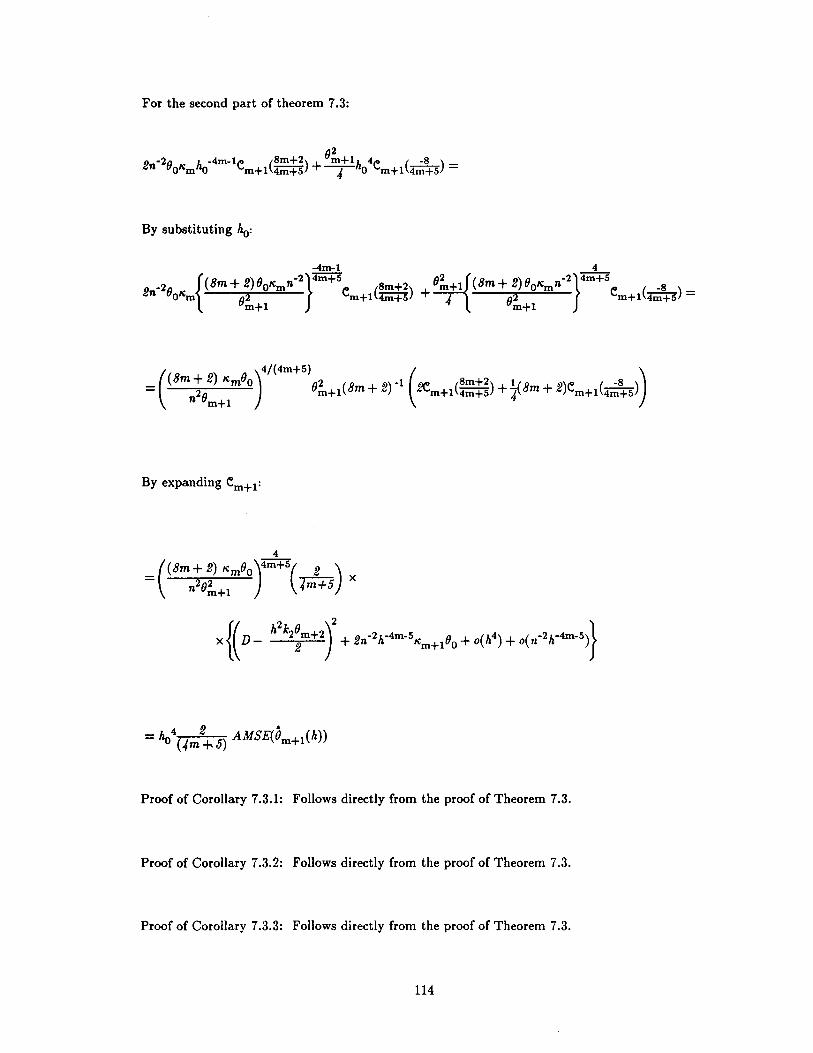
For the second part of theorem 7.3:
(J26) -2(J h -4m-l", (8m+2) + m+lh 4", (-8) _",n OlCm 0 '"'m+l 4m+5 -4- 0 '"'m+l 4m+5 -
By substituting ho:
By expanding em +!:
42'= ho (4m +5) AMSE((Jm+!(h»
Proof of Corollary 7.3.1: Follows directly from the proof of Theorem 7.3.
Proof of Corollary 7.3.2: Follows directly from the proof of Theorem 7.3.
Proof of Corollary 7.3.3: Follows directly from the proof of Theorem 7.3.
114
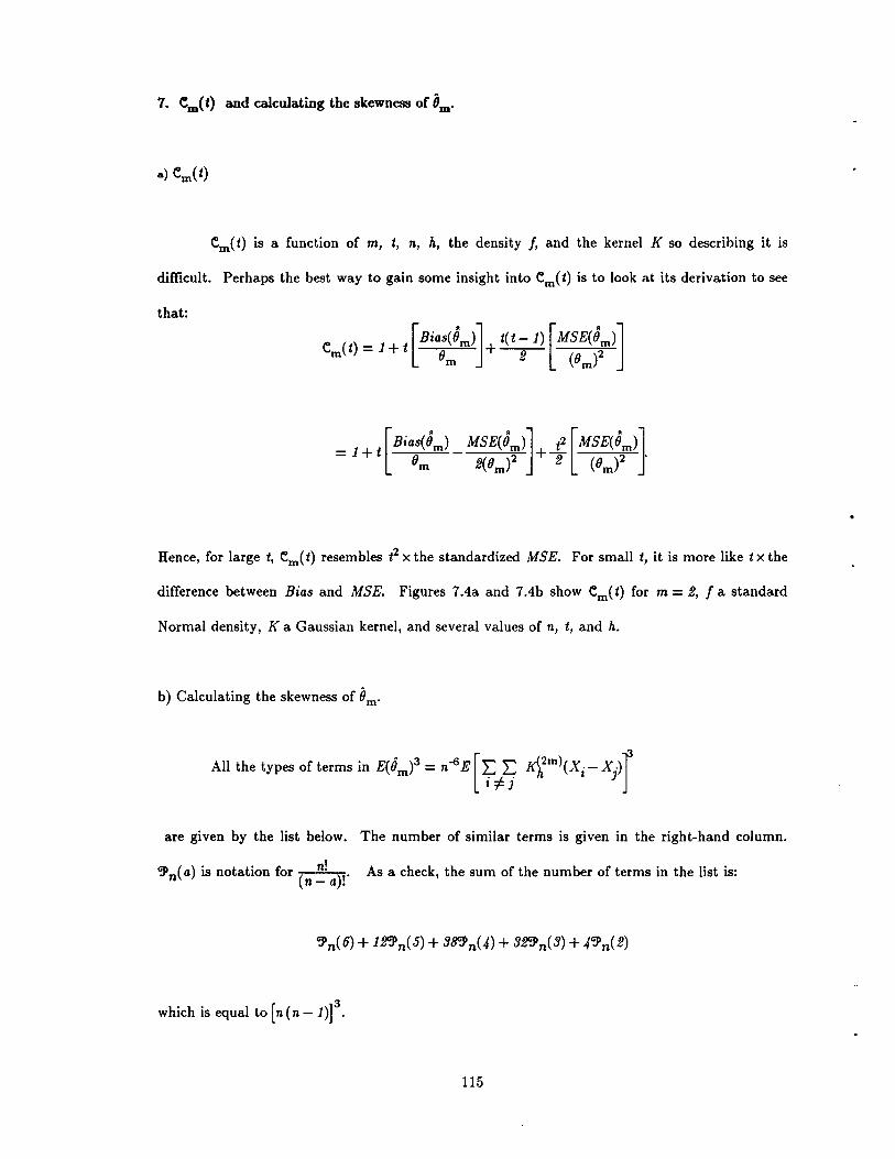
7. em ( t) and calculating the skewness of 8m .
em(t) is a function of m, t, n, h, the density f, and the kernel K so describing it is
difficult. Perhaps the best way to gain some insight into em(t) is to look at its derivation to see
that:
Hence, for large t, em(t) resembles t2 x the standardized MSE. For small t, it is more like t x the
difference between Bias and MSE. Figures 7.4a and 7.4b show em(t) for m = 2, f a standard
Normal density, K a Gaussian kernel, and several values of n, t, and h.
b) Calculating the skewness of 8m .
are given by the list below. The number of similar terms is given in the right-hand column.
~n(a) is notation for (n~! a)r As a check, the sum of the number of terms in the list is:
which is equal to [n(n-l)t
115
Term: Given by: Number:
E{ R),2m)(Xl - X2)R),2m)(X3 - X4)R),2m)(Xs - X6)} Ej ~n(6)
E{ R),2m)(Xl - X2)Rfm)(X3 - X4)R),2m)(Xl - Xs)} E2 j~n(5)
E{ R),2m)(Xl - X2)R),2m)(X3 - X4 )Rfm)(X3 - X4)} E3 ~n(4)
E{ R),2m) (Xl - X2)R),2m)(Xl - X3)R),2m)(Xl - X4 ) } E4 sc:P n(4)
E{ Rfm)(Xl - X2)R),2m)(Xl - X3 )R),2m)(X2- X4)} E5 24~n(4)
E{ R),2m)(Xl - X2)R),2m)(Xl - X2)R),2m)(Xl - X3 )} E6 24~n(3)
E{ R),2m) (Xl - X2)R),2m)(Xl - X2)R),2m)(Xl - X2)} E7 4~n(3)
E{ R),2m)(Xl - X2)R),2m)(Xl - X3 )R),2m)(X2- X3)} ES sc:P n(2)
116
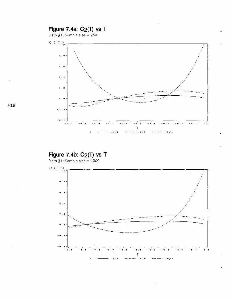
Figure 7.4a: C2(1) vs TDistn #1; Sample size = 250
:klW
C ( T )1 .0
0.8
0.8
0.4
0.2
0.0
I
;\ ;\ ;\ ;\ ;\ ;\ ;
\ /\ /
\ I\ I~ I, /, /, /
' ............. , - - - - /,./-'- - - - - - - u _
..... ,---,=:.:.:~:':':-::"=--------=7~"-· --------
J -~-_--.- •••• - •••• - ••••" ..:c.-~~=----.-.-.---// --.. _------
-0.2
- 0 . 4 ""-r--~-___r----,__---_,_---.,..-----r---__,----,_---..,_---__,-~-___,J
- 1 • 0 - 0 . 9 -o.a -0.7 -0.6 -a.S -0.4 -O.J -0.2 - 0 . 1 0.0
T--- -2/0 -------- - .. / 9 ----- 10/9
Figure 7.4b: C2(1) vs TDistn #1; Sample size = 1000
---
I;;
;;
;;
;/
//
I;'
//
/-- --- ------------~~:7'-------- --- _
.-_.--------
.-.... .. --- ...- ..--------------
o . 2
o . 4
0.0
0.8
0.8
C ( T ).0
- 0 . 2
0.0- 0 . 1- a . 2-0.3- 0 . -4-0.3-0.6- 0 . 7-0.8- 0 . 9
- 0 . • "'r---__,----,------,-----,----...,.---__,r-----,_---..,_---__,---___,J- 1 .0
T--- -2/51 -------- - -4 / 9 ----- 10/9
Chapter VIll: The "K-Step" Estimator
1. Introduction.
In the previous chapter, a "one-step" estimator was introduced. The "one-step"
estimator is a kernel estimator of ()m with a bandwidth containing an estimate of ()m+!" The
estimate of ()m+! is another kernel estimator depending on some bandwidth.
The obvious extension to the "one-step" estimator is the "k-step" estimator. Suppose
that ()m is to be estimated. The AMSE optimal bandwidth for this estimation problem is a
function of ()m+l. The "one-step" estimator substitutes a smoothing estimate of ()m+! into this
optimal bandwidth. This bandwidth is used to provide a smoothing estimate of ()m. Of course,
this process can be extended so that the initial functional estimated is ()m+k" This is used to
estimate ()m+k-l' which is used to estimate ()m+k-2' and so on. This is the "k-step" estimator.
The "one-step" estimator discussed in chapter VII was a leave-out-the-diagonals
estimator. The estimator used to estimate the bandwidth was a leave-in-the-diagonals
estimator. An obvious question is how does the "one-step" estimator discussed in the previous
chapter compare to a "one-step" in which both estimators are leave-in-the diagonals estimators.
This "one-step" estimator is discussed in this chapter as a special case, although the bandwidth
used here is stochastic rather than selected as it was in chapter VII.
By the previous chapter, the "Sheather-Jones" optimal bandwidth for estimating 8m is
given by:
Recall that the "Sheather-Jones" bandwidth is not the asymptotic MSE optimal
bandwidth, but merely the bandwidth that eliminates the first term in the Taylor expansion of
the bias.
Of course, the process of "stepping" must stop somewhere, so there is some initial
bandwidth decision to be made. It seems reasonable to expect that "stepping" should mitigate
the impact of a poor initial bandwidth. One possible choice for an inital bandwidth is to "plug-
in" the Gaussian density into the expression for the AMSE optimal bandwidth. Notice that if a
Normal kernel is used:
{
-1 }1/2m+32 n •= 2m+l (J'
which is slightly less than n-1/ 2m+3 fT.
119

The "k-step" estimator discussed in this chapter uses the "plug-in" bandwidth as its
initial bandwidth. This makes the discussion a bit easier than in the previous chapter since
here, the estimator relies only on integer k, rather than a bandwidth.
2. Assumptions and Notation.
Define:
(5.1)
where 0m+l is an estimator of Om+!' If
then hm is a "plug-in" or "O-step" bandwidth and we will write hm == h~, However, if
Om+! == O~+! is a "k-step" kernel estimator then h~+! is a "(k+l)-step" bandwidth.
In this chapter, Om is a "leave-in-the-diagonals" estimator of Om so it is always positive.
To avoid some technical problems, we assume that it is bounded away from 0 a.s.. This is not
a large assumption because we usually worry about Om being too large rather than too small. In
any case, Om is bounded away from 0 a.s. if any measure of sample variability is bounded a.s..
..
120
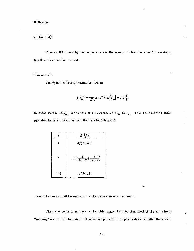
3. Results.
Oka. Bias of Om.
Theorem 8.1 shows that convergence rate of the asymptotic bias decreases for two steps,
but thereafter remains constant.
Theorem 8.1:
Let 0;:' be the "k-step" estimator. Define:
In other words, I3(Om) is the rate of convergence of EOm to Om. Then the following table
provides the asymptotic bias reduction rate for "stepping".
k I3(O~)
0 -2/(2m+3)
1 -2X(2rrf+3+ 2rrf+5)
~2 -4/(2m+3)
..
Proof: The proofs of all theorems in this chapter are given in Section 6.
The convergence rates given in the table suggest that for bias, most of the gains from
"stepping" occur in the first step. There are no gains in convergence rates at all after the second
121
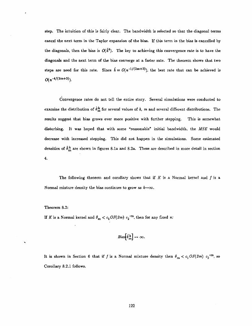
..
step. The intuition of this is fairly clear. The bandwidth is selected so that the diagonal terms
cancel the next term in the Taylor expansion of the bias. If this term in the bias is cancelled by
the diagonals, then the bias is 0(h4). The key to achieving this convergence rate is to have the
diagonals and the next term of the bias converge at a faster rate. The theorem shows that two
steps are need for this rate. Since h= O(n-1/(2m+3)). the best rate that can be achieved is
O( n-4/(2m+3)).
Convergence rates do not tell the entire story. Several simulations were conducted to
examine the distribution of 8~ for several values of k, m and several different distributions. The
results suggest that bias grows ever more positive with further stepping. This is somewhat
disturbing. It was hoped that with some "reasonable" initial bandwidth, the MSE would
decrease with increased stepping. This did not happen in the simulations. Some estimated
densities of 8~ are shown in figures 8.1a and 8.2a. These are described in more detail in section
4.
The following theorem and corollary shows that if K is a Normal kernel and f is a
Normal mixture density the bias continues to grow as k-+oo.
Theorem 8.2:
If K is a Normal kernel and Om < C1 0 F( 2m) c2-m. then for any fixed n:
Bia{B~] -+ 00•
It is shown in Section 6 that if f is a Normal mixture density then Om < c1 0F(2m) c2-m , so
Corollary 8.2.1 follows.
122
Corollary 8.2.1:
If K is a Normal kernel and fis a Normal mixture density, then for any fixed n:
Bia{O~] --> 00.
The significance of this result is that the MSE of the "k-step" estimator must also go to
infinity as Ie increases. This obviously implies that continued stepping is not a good plan. The
theorem can probably be made more general, although this was not explored. The corollary is a
counter-example to the hypothesis that continued stepping may be a good plan. This is
formalized in the following corollary.
Corollary 8.2.2:
If K is a Normal kernel and fis a Normal mixture density, then for any fixed n:
MSE[O~] --> 00.
Stepping primarily affects the difference between the diagonal term and the next term in
the expansion of the bias. This difference can be decomposed into a positive and a negative
term. Stepping causes the positive term to grow, basically by making the bandwidth smaller.
The n~gative term represents the bias of 8~+k multiplied by (Ie - 1) bandwidths. The negative
term gets smaller by this multiplication.
The divergent series in the proof of Theorem 8.2 provides some intuition into how the
bias behaves. Notice the series is something like E i'(1/n)'. When n is large, the series seems
to converge for the first few steps. Notice also that the larger is n, the higher number of steps
must be taken to cancel the negative term. Hence, with very large n, "stepping" more than 2
steps may continue to reduce bias. The intuition here is that with a tremendous sample size it
123
is possible to estimate many of the 0i's productively.
a. Variance of B~.
"Stepping" does not affect the order of convergence of the variance.
Theorem 8.3:
Let B~ be the "k-step" estimator. Then, for any k:
Once again, convergence rates are not the complete story. It seems reasonable to expect
that with each step taken more variance is added to the final estimator. This intuition turns
out to be correct and it is formalized in the following theorem.
Theorem 8.4:
Let B~ be the "k-step" estimator. Then, for any k, Var(O~) is an increasing function of k.
Oka. MSE of Om.
Mimicing Theorem 8.1, define:
So ,(Bm) is the rate of convergence of MSE[Om] to O. Combining Theorems 8.1 and 8.2 shows
124
that the MSE error convergence rate is given by the following table:
k ;(8~)
0 -4/(2m+3)
~1 -5j(2m+3)
4. Simulations.
Simulations provide some useful insights into the behavior of the k - step estimators.
The asymptotic calculations imply that the MSE convergence rate of the estimators improves for
the first step. The bias convergence rate improves for the first two steps. However, both bias
and variance eventually grow without bound with further stepping. An aim of the simulations
is to investigate in several practical cases the optimal number of steps to minimize the MSE.
The simulations were done on distributions 1- 6, 10, and 11. For each simulation, (Jl
was estimated. In all cases, all the estimators from the "0 - step" to the "20 - step" were
computed. All simulations were done using the same seed and 100 samples. Sample sizes of 100
and 500 were investigated. Only simulations from distributions 3 and 6 are presented here as
they seem to be representative of all the conclusions discussed below.
Results that confirm the theoretic calculations are:
• The biggest gains in estimation occur during the first two steps. Thereafter, the estimator
either got worse or improved only slightly with each step.
• The larger the sample size, the greater the number of steps should be taken.
• The bias and variance of the estimator both eventually grow with increased stepping.
125
Results not apparent from theoretic calculations are:
• The final bandwidth computed became more variable and had a mean that steadily
approached 0 with increased stepping.
• The more non-Normal the distribution (i.e., the more different the sequence of 9i from that of
the Normal distribution), the more steps were required to the optimal.
Figure 8.1a shows an estimated density of lit for distribution 6. The density at the far
left is the "0 - step" and steps increase to the right. 1t is clear that the estimates get
increasingly variable with increasing k. Further, the means of the distribu tions initially get
closer to the true value and then keep increasing past it. The largest gains are found in the
first two steps.
Figure 8.1b shows the estimated densities of the bandwidth used in the final estimate of
91, The density at the far right is the "0- step" density and steps increase to the left. The
mean of the density steadily approached O. The variance of the density also increased.
Figures 8.2a and 8.2b are similar to 8.1a and 8.1b except that density 3 is used rather
than density 6. Density 3 is much more non-Normal and this difference is reflected in the litand bandwidth densities. It takes many steps before EIi~ is less than 9\. Further, the expected
value of the bandwidth does not become less than the optimal bandwidth even after twenty
steps. The insight is that the optimal bandwidth is much less than the plug-in bandwidth from
the Normal so it takes many steps to reach the optimal.
Figures 8.3a and 8.3b are plots of the standardized MSE for distribu tion 6 and sample
sizes of 100 and 500. The graphs show that with a sample size of 100, the MSE is minimized
with 1 step. With a sample size of 500, the minimum MSE is attained after 2 steps. This
increased number of steps with increased sample sizes coincides with the theoretic result
126
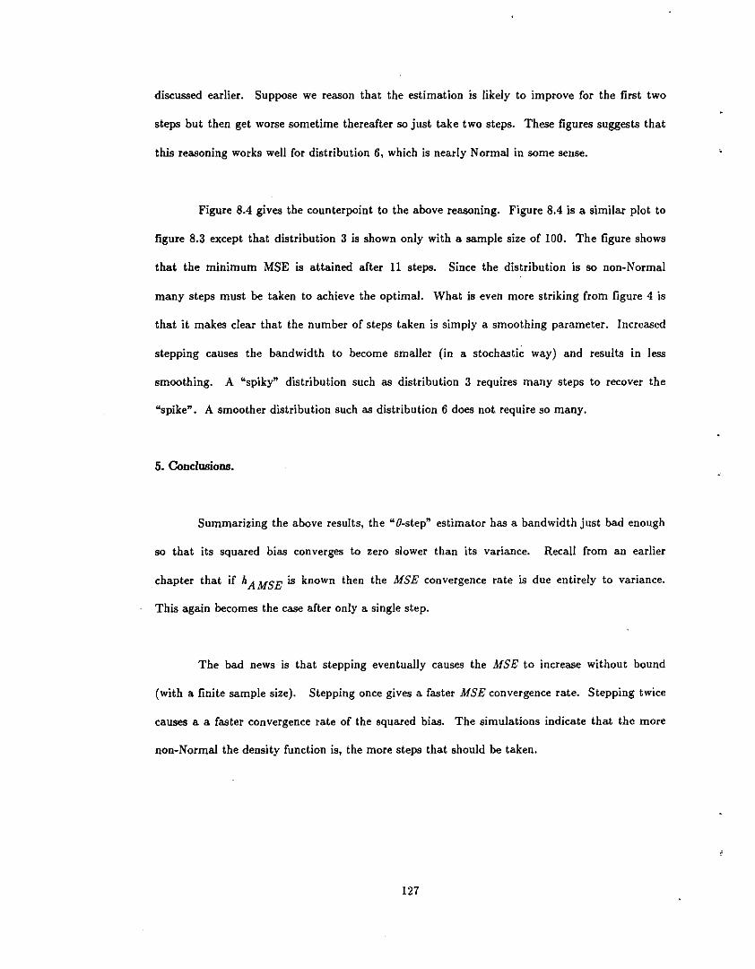
discussed earlier. Suppose we reason that the estimation is likely to improve for the first two
steps but then get worse sometime thereafter so just take two steps. These figures suggests that
this reasoning works well for distribution 6, which is nearly Normal in some sense.
Figure 8.4 gives the counterpoint to the above reasoning. Figure 8.4 is a similar plot to
figure 8.3 except that distribution 3 is shown only with a sample size of 100. The figure shows
that the minimum MSE is attained after 11 steps. Since the distribution is SO non-Normal
many steps must be taken to achieve the optimal. What is even more striking from figure 4 is
that it makes clear that the number of steps taken is simply a smoothing parameter. Increased
stepping causes the bandwidth to become smaller (in a stochasti~ way) and results in less
smoothing. A "spiky" distribution such as distribution 3 requires many steps to recover the
"spike". A smoother distribution such as distribution 6 does not. require so many.
5. Conclusions.
Summarizing the above results, the "O-step" estimator has a bandwidth just bad enough
so that its squared bias converges to zero slower than its variance. Recall from an earlier
chapter that if hAMSE is known then the MSE convergence rate is due entirely to variance.
This again becomes the case after only a single step.
The bad news is that stepping eventually causes the MSE to increase without bound
(with a finite sample size). Stepping once gives a faster MSE convergence rate. Stepping twice
causes a a faster convergence rate of the squared bias. The simulations indicate that the more
non-Normal the density function is, the more steps that should be taken.
127
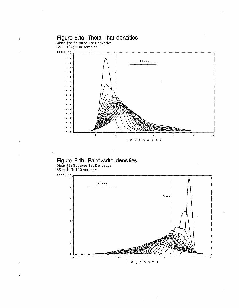
Figure 8.1a: Theta- hat densitiesDisln #6; Squared 1sl DerivativeSS = 100: 100 samples
D [loIS; ~ j .r----------...,--------------------------,, .., . ,, .., . J
, . ,,. ,, .0
o . ,
0.'
o. ,
o .•
o . ,
0 .•
O. J
o . ,
-. _ J -, o
n ( the to)
Figure 8.1b: Bandwidth densitiesDistn #6; Squared 1st DerivativeSS = 100: 100 samples
ot N S , r; .r------------------------...,-----------.,
•
1 n ( h hat )
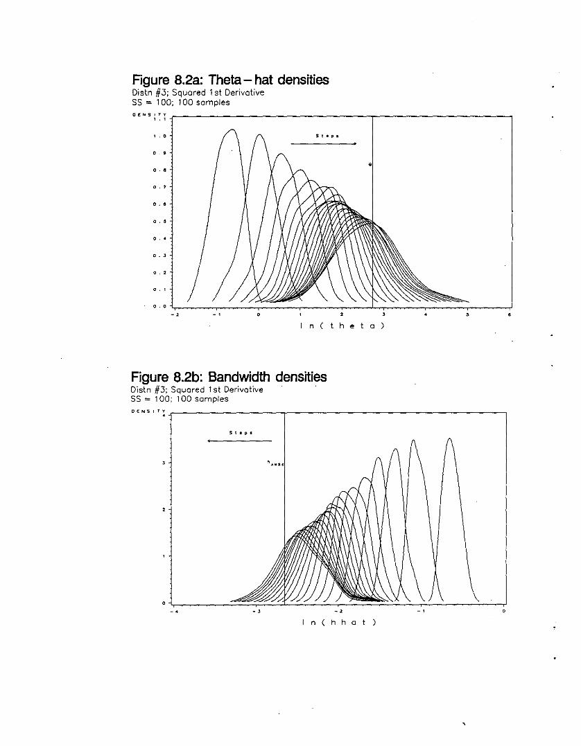
Figure 8.2a: Theta - hat densitiesDistn #3; Squared 1st Derivative55 = 100; 100 samples
o t NS i ~ i -r------------------,--------------,
, . 0
o •
o .•
0.'
o .•
o . ,
o .•
o. ,
o . ,
o . ,
-, o ,n ( the t a )
• •
Figure 8.2b: Bandwidth densitiesDistn #3; Squared 1st Derivative .5S = 100; 100 samples
DEN 5 I T ~ -r----------,---------------------,
-. -, -,I n ( h hat )
- ,
,
o
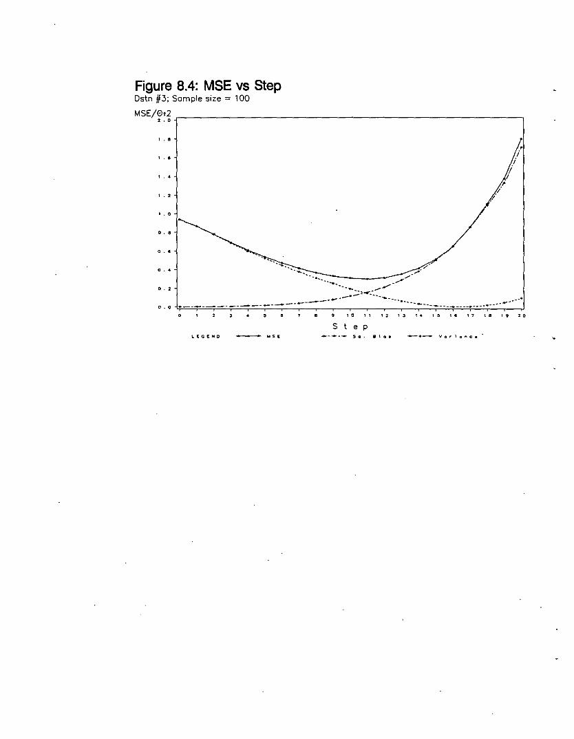
Figure 8.4: MSE vs StepDstn #3; Sample size = 100MSE/Pt~ .,-- --,
·...· ,
· 0
o .•
o .•
0.'
,i
ii
I,i
.i
0.'.......•. .....,/
__ _I"'"-------_..::: .....~..__....•_---_. .,.o . 0 -<;."-=·"-T='·o~=~-=o·,-=.:·;-:::;:;-=.:·c-;=.·--~----·~-~-~--~-~-~~-~-~_·c·c-;:..:·"·o·"-c·o·o·"·~·;·;·;·"·T··-·-·-·--~·-·_,J
o • • • I Q 1 1
S t e p
12 13 ,. ,~ 16 17 18 19 2.0
_loiS!!: _- SQ. B I ... _e_ v" ~ 1 "", c:.
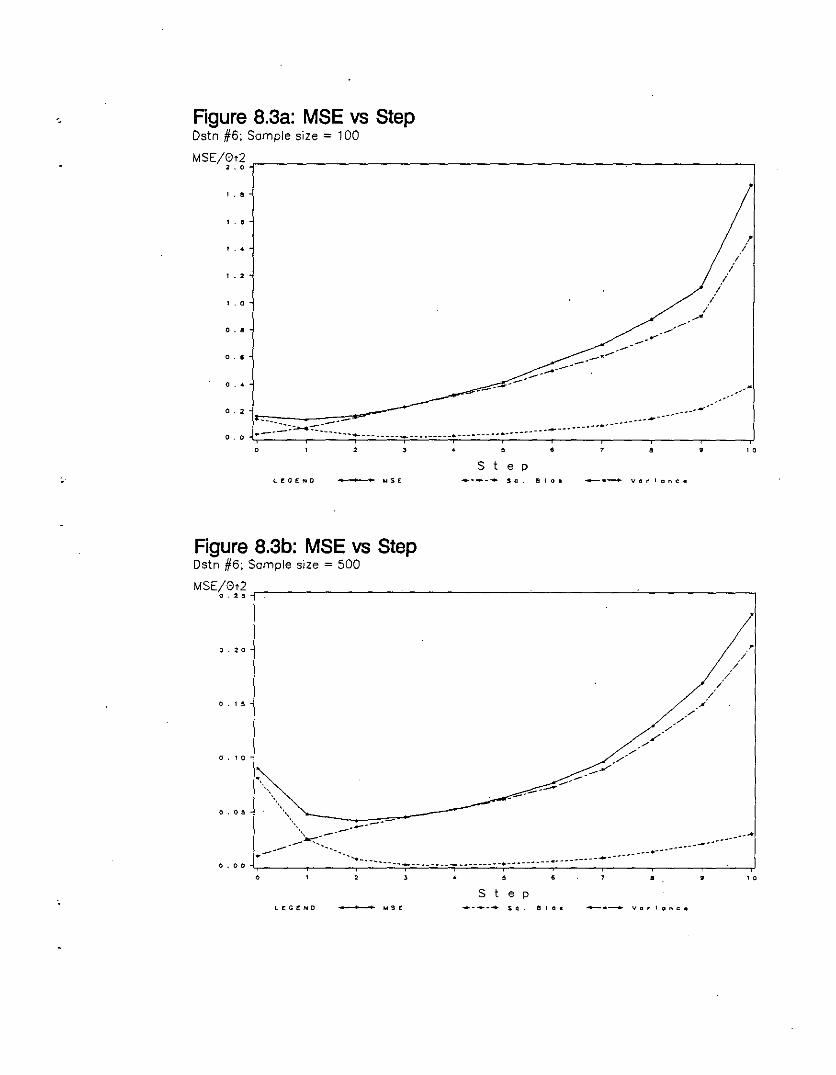
'. Figure 8.3a: MSE vs StepDstn #6; Sample size = 100
MSE/~t~ .,- -------..,
. ,
.,
..
. ,
.0
o.
o.
0.'
o .
-~----
,;/
/I
;;
;.-'
./.-/
.---0.0
o , , , , ,S t e p
LEGENO _ ~SE +--.- SQ 6 I " • _ .. _ Va,. Ion".
Figure 8.3b: MSE vs StepOstn #6; Sample size = 500
MSE~0:~ ..- ~ ~ ~ __,
o . 1.5
,/
///
/J
//
/..-/
..--
o . 10
o.oa
..."\,
\\\"
, -------;.~-~
.-~- '~, --o. 0 a"-c ~-----·~------------c-c-,-o-O-C-C-"-"-"-"-"-c-O-O-C-C-"-"-"-C-r·c--_-_-_-_-_-_-_-"·_-_--_-_-_-_-_-,-_-~----------------,.------~-~-,J
o , , , •S t e p
LEGENO _""lOl!: ----- SQ B I " •
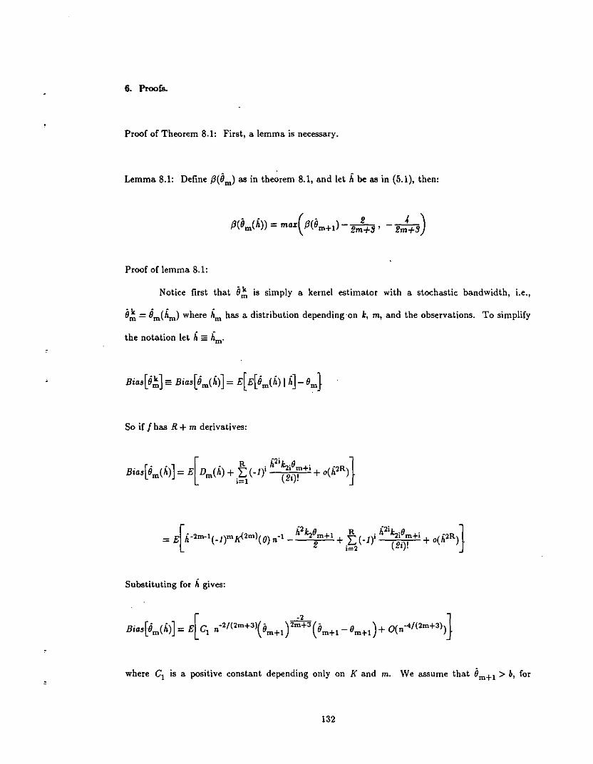
6. Proofs.
Proof of Theorem 8.1: First, a lemma is necessary.
Lemma 8.1: Define f3(Om) as in theorem 8.1, and let h be as in (5.1), then:
Proof of lemma 8.1:
Notice first that 0;:' is simply a kernel estimator with a stochastic bandwidth, Le.,
0:' = tim(~) where ~ has a distribution depending on k, m, and the observations. To simplify
the notation let h;: hm'
So if f has R + m derivatives:
Substituting for hgives:
where C! is a positive constant depending only on K and m. We assume that 0m+! > b, for
132
some positive bound b. Hence,
The lemma follows immediately.
Proof of Theorem 8.1:
.' ·'0 . .2/(2m+5) • 2If k= 1, then Blas(8m+1) = Blas(8m+1) = O(n ) by the above so 13(8m+I) = - 2m+ 5'
If k = 2, then Bias(Om+I) = Bias(O:"+I) = 0(n·2/(2m+5) x n'2/(2m+7) by th~ above. Since
i~ 2m':" + I < - 2m"+ 5 for k ~ 2, the ditTerence between the diagonals term and the first
term in the expansion of the bias is not as large as the next term in the expansion. Hence,
Proof of Theorem 8.2: Several lemmas are necessary.
Lemma 8.2:
Let SOt =f: (_l)k+i kOt( i + k)!( 2n - i - k)!k=O [( n - k)! kIf
Then Ot =0 SOt =1.
Ot =1 SOt =- n2 + (2n + 1) i
Ot =2 SOt =+n2 (n - 1)2 - n (2n + 1)(n -1) i + n(2n + 1) ;2
Proof of lemma 8.2: Prudnikov, et. aI. (1986).
133
Lemma 8.3:
n (n)2Let To- = LIPt=O
Theno-=O
0-=1
0-=2
To- = (~)
To-=(~) 2T =(2n- 2) n2
0- n-1
Proof of lemma 8.3: Prudnikov, et. al. (1986).
Lemma 8.4:
( m+2)(m+2)_ m m ;+j (m) m i + 1 j + 1 _ (m + 2)2
Qm-i~j~(-l) i (j) (.2m+ 4 ) -2(2m+1)(2m+S)'. 1+1+ 2
Proof of lemma 8.4:
( m+ 2)(m+ 2)Qm=I:I:(-li +j (m)(m) i+1 ;+1
;:OJ:o 1 1 (.2m+ 4 )1+1+ 2
Substituting 1= i + 1, 5 = j + 1, n = m + 2 and expanding the combinations gives:
Q_ (n!)2 ~ (n - I) I ~ ()'+5( 2) (2n - 1- 5)! (I + 5)!
2- L. L. -1 n5-Sn- (2:) n2( n _1)2 ':1 [( n - I)! I!f 5:1 [( n - 5)! 5!f
134
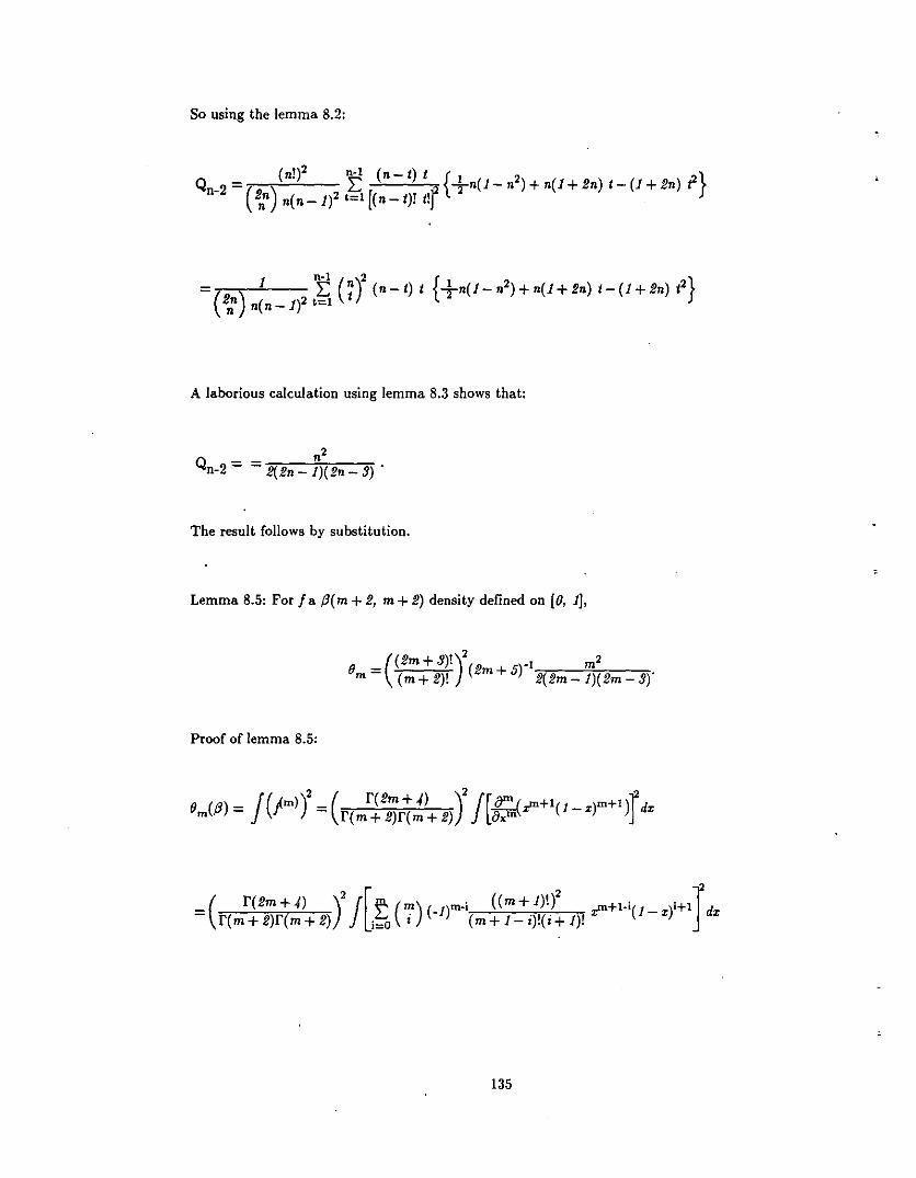
So using the lemma 8.2:
(n f? n-I (0 I) I { }Qn-2 = ( ). E - f +0(1- n
2) + n(1 + 2n) I - (1 + 2n) r-
2nn n( n - 1)2 '=1((n - I)! II
A laborious calculation using lemma 8.3 shows that:
n2
Qn-2= = !!(20 1)(20 3)·
The result follows by substitution.
Lemma 8.5: For fa 13( m + 2, m + 2) density defined on [0, 1],
((2m+3)!)2 .1 m2
°m= (m+2)! (2m+5) !!(2m-1)(2m-3)"
Proof of lemma 8.5:
o(13) =J(fm))2 =( r(2m+4) )2J[~z"'+I(1_x)m+l)rdXm r(m+ 2)r(m+ 2) oxm
(r(2m+4) )2J[~ (m) m-i ((m+1)!)2 +I.i i+IJ= rem + 2)r(m + 2) ;=0 i (-1) (m+ 1- i)!(i+ 1)! z'" (1- x) dx
135
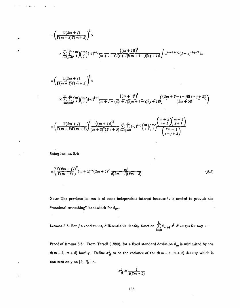
(f(em+ 4) )2
= f(m+ e)f(m+ e) X
m m(m)(m) Hi (m+l)!t j;m+20ioi i+;+2xEE· . (-1) ( +1 "l'C+1)'( +1 ")'("+1)' (l-x) dxi=Oj=O '1m - J • I • m - 1 . 1 .
(f(em+ 4) )2
= f( m + e)f(m + e) x
m m(m)(m) i+i (m+l)!tx i~i~O i j (-1) (m + 1- i)!( i + 1)!(m+ 1 -j)!(j + 1)!
(em + e- i - J")!(i + j + e)!)(em+ 5)!
( m+eXm+e)_( f(em+4) )2 (m+l)!)2 m m _ i+i(m) m i+l j+l- f( m+ e)f(m+ e) (m + e)2(em + 5) i~i~ ( 1) i (j) ( .em + 4 )
'+J+ e
Using lemma 8.4:
·(f(em + 4»)2 -2 _\ m2= f(m + e) (m + e) (em + 5) e(em -1)(em _ 3) (801)
:
Note: The previous lemma is of some independent interest because it is needed to provide the
"maximal smoothing" bandwidth for Om-
k .Lemma 8.6: For f a continuous, differentiable density function L: 0m+i a1 diverges for any a.
i=O
Proof of lemma 8.6: From Terrell (1990), for a fixed standard deviation Om is minimized by the
13(m+ e, m+ e) family_ Define q~ to be the variance of the 13( m+ 2, m+ 2) density which is
non-zero only on [0, 1], i.e.,
q2 _ 113 - 4(em+ 5)
136
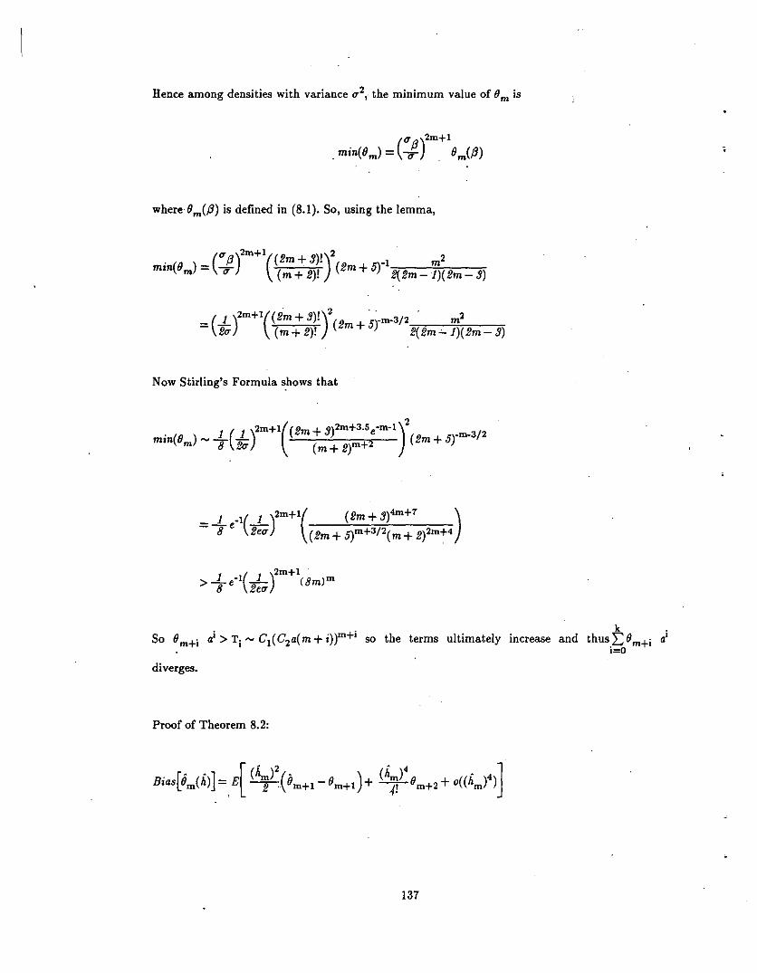
Hence among densities with variance u 2" the minimum value of 8m is
whereUm(.8) is defined in (8.1). So, using the lemma,
. (Uf3)2rn+1(( tim + 3)!)2 .1 m2mln(Um) = "7 (m+ til! (tim + 5) ti(tim-1)(tim- 3)
. 2 . . .
(1 )2rn+1(( tim + 3)!) -rn-3/2 m2
= tiu (m + til! (tim + 5) tie tim "-1)( tim - 3)
Now Stirling's Formula shows that
( )
22m+l 2m+3.5 ·m-lmineU ) ~ ...L(.1..) (tim + 3) e (tim + 5rm-3/ 2
m 8 tiu (m+ tir+2
1 '1( 1 )2m+1( (tim + 3)4m+7 )= 8 e tieu (tim + 5)m+3/2(m + ti)2rn+4
( )2rn+1>...L e-1 _1_ (8m)m
8 tieu
diverges.
Proof of Theorem 8.2:
137
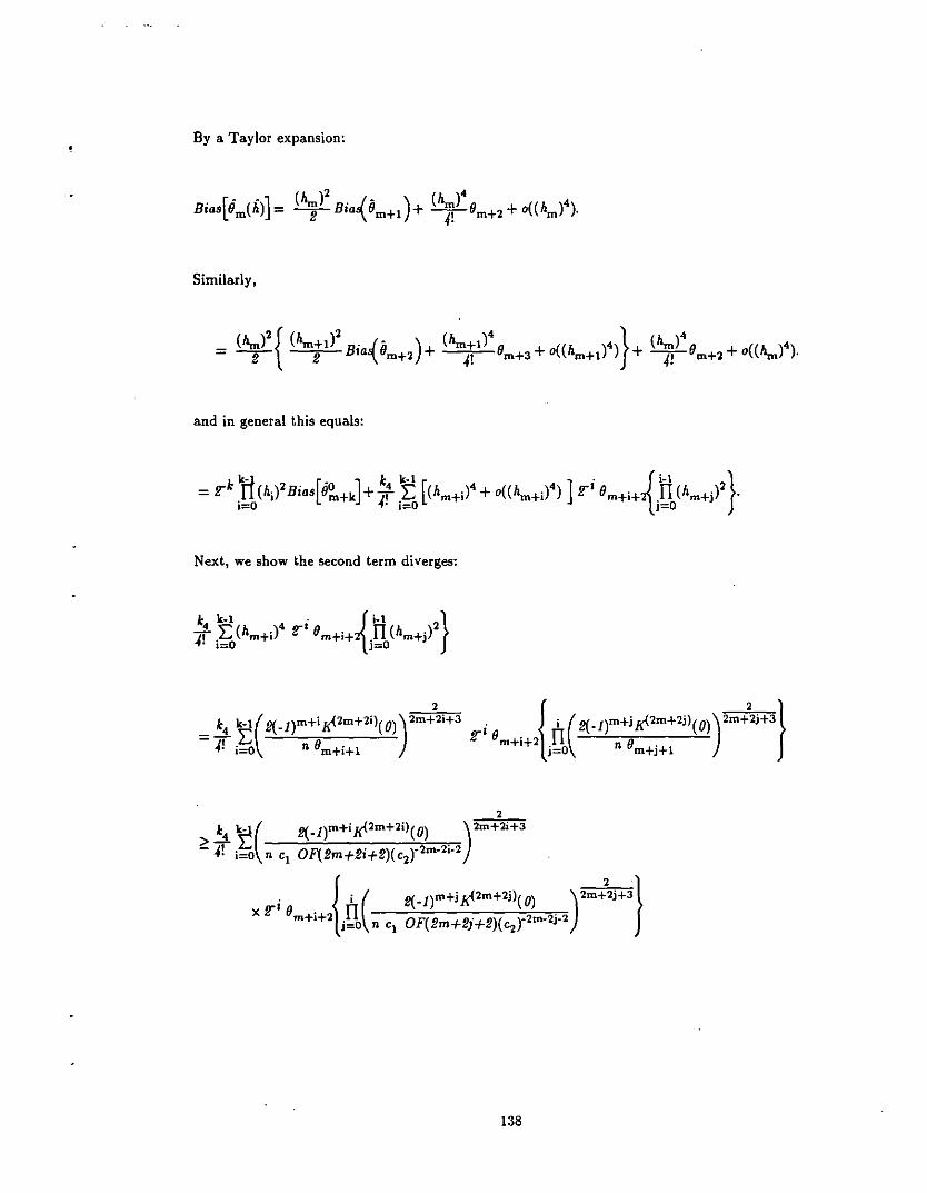
By a Taylor expansion:
Similarly,
and in general this equals:
Next, we show the second term diverges:
2
=k4 E(e<_Jlm+ij(l2m+2i)(Ol)2m+2i+3
~! i=O n 8m+i+l
2
138
2
= k4 k.l( 20F(2m+2i)(!brr1/2 )2m+2i+3-I! i~ n C1 OFf 2m+2i+2)(C2r2m.2i-2
{
2 }Xfri 0 i 20F(2m+2j)(21rr l / 2 2m+2j+3m+i+2 jU(n C
1OF(2m+2j+2)(c2r2m-2j.2)
where "J and c4 depend only on m and f. This series diverges as a consequence of lemma 8.6.
Proof of Corollary 8.2.1:
t
If /is a Normal mixture density then j(x) = L:Pi <Pu,(x-I';) so:. i=l I
139
By Cauchy-Schwarz:
The corollary follows immediately.
Proof of Corollary 8.2.2:
This is a direct consequence of Corollary 8.2.1.
Proof of Theorem 8.3:
Regarding the "k-step" estimator as a standard kernel estimator with a stochastic
bandwidth gives:
For the first term,
140
So,
4Var(0m(h)) Ih] = Cn·5/(2m+3)e[Om+!fm
+!)/(2m+3)
[_ ,<4m+!)/(2m+3)
Since E 0m+lJ =0(1) for any kernel estimator,
For the second term,
{ h2] {-4 ]:s Va ~m+! + Va O(h)
t( ."2) ,)2/(2m+3) ]=Va 2(.1)m
l\.' rn (O)n' 8'2+1 + 0(n.8/{2m+3»)
~8m+!
{d ).4/(2rn+3) [d )'2/{2m+3)]2}" ""= Cn .4/{2rn+3) "\Om+! - "\Om+! + O( n .8/(2m+3»)
If the bandwidth used in 8m+! is 0(n' /(2m+5»). then Lemma 7.1 in the previous chapter implies:
{d' ).4/(2m+3) _[d - )'2/(2m+3)]2} _ -2/{2m+5)",8m+1 ",8m+! - O(n ).
Hence,
The theorem follows by combining the two terms.
141

-.'
Proof of Theorem 8.4:
As in the proof of theorem 8.3:
-5!(2m+3) [- 14m+ll!(2m+3l;:: Cn E 0m+l
[_ "j!4m+ll!(2m+3)
for some positive C. But by Theorem 8.2, E 0m+lJ - 00 as k - 00.
142

APPENDIX A: GAUSSIAN MIXTURE DENSITIES
Note: The figures in Appendix A were taken from Marron and Wand (1991).
viii
S. T. Sheather and M. C. Jones (1989), "Reliable data-based bandwidth selection for kernel
density estimation, with emphasis on a successful 'non·cross validatory' approach," Unpublished.
manuscript.
T. Schweder (1975), "Window estimation of the asymptotic variance of rank estimators of
location," Scand. J. Statist., vol. 2, pp. 113-126.
G..R. Terrell (1990), "The maximal smoothing principle in density estimation," Jour. of Am.
Statist. Ass., vol. 85, pp. 47Q..477.
B. van Es (1988), "Estimating functionals related to a density by a class of statistics based on
spacings," To appear.
W. Wertz (1981), "A remark on the estimation of functionals of a probability density," Prob.
Contr. Info"". Theory, vol. 10, pp. 279-285.
xiv
•
,
•
,
•
A. Miura (1985), "Spacing estimation of the asymptotic variance of rank estimators of location,"
Proceedings of the Indian Statistical Institute Golden Jubilee International Conference on
Statistics: Applications and other Directions, pp. 391-404.
H. G. Muller (1984), "Smooth optimum kernel estimators of regression curves, densities, and
modes," Ann. Statist., vol. 12, pp.766-774.
E. Parzen (1962), "On estimation of a probability density and mode," Ann. Math. Statist., vol.
33, pp. 1065-1076.
M. Pawlak (1986), "On non parametric estimation of a functional of a probability density,"
IEEE Trans. Info. Th., vol. IT-32, no. 1, pp. 79-84.
B. L. S. Prakasa-Rao (1983), Nonparametric Functional Estimation, Academic Press, N.Y..
A. P. Prudnikov, Yu. A. Brychkov, O. 1. Marichev (1986), Integrals and Series Vi, Gordon and
B~each, N.Y..
Y. Ritov and P. J. Bickel (1987), "Achieving information bounds in non and semi-parametric
models," To appear in A nn. Stat.
E. F. Schuster (1974), "On the rate of convergence of an estimate of a functional of a
probability density," Scand. Actuarial J., vol. 2, pp. 103-107.
D. W. Scott and S. J. Sheather (1985), "Kernel density estimation with binned data," Comm. in
Statist. • Theor. and Meth., vol. 14, pp. 1353-1359.
D. W. Scott and G. R. Terrell (1987), "Biased and unbiased cross-validation in density
estimation," Jour. of Am. Statist. Ass., vol. 82, pp. 1131-1146.
W. R. Schucany and J. P. Sommers (1984), "Improvement of kernel type density estimators,"
Journal of the American Statistical Association, vol. 72, 420-423.
xiii
H. L. Gray and W. R. Schucany (1972), The Generalized Jackknife Statistic, New York: Marcel
Dekker.
P. Hall (1982), "Limit theorems for estimators based on inverse of spacings of order statistics,"
Ann. Prob., vol. 10, pp. 992-1003.
P. Hall and S. Marron (1987), "Estimation of integrated squared density derivatives," Stat. (3
Prob. Let., vol. 6, pp. 109-115.
1. Hodges and E. Lehmann (1956), "The efficiency of some nonparametric competitors of the t
test," Ann. Math. Stat., vol. 27, pp. 324-335.
M. C. Jones (1989), "Discretized and interpolated kernel density estimates," Jour. of Am.
Statist. Ass., vol. 84, pp. 733-741.
M. C. Jones and H. W. Lotwick (1983), "On the errors involved in computing the empirical
characteristic function, n Journal of Statistical Computation and Simulation, 17, 133-149.
H. L. Koul, G. L. Sievers, and J. McKean (1987), "An estimator of the scale parameter for the
rank analysis of linear models under general score functions," Scand. J. Statist., vol. 14, pp. 131
141.
E. L. Lehmann (1963), "Nonparametric confidence intervals for a shift parameter," Ann. Math.
Stat., vol. 27, pp. 1507-1512.
T. Lissack and K. S. Fu (1976), "Error estimation in pattern recognition via La-distance
between posterior density functions," IEEE Trans. Info. Th., vol. IT-22, pp. 34-45.
J. S. Marron (1988), "Automatic smoothing parameter selection," Emp. Econ., vol. 13, pp. 187
208.
J. S. Marron and M. P. Wand (1991), "Exact Mean Integrated·Squared Error," Annals of Stat.,
To appear.
xii
;
REFERENCES
I. A. Ahmad (1976), "On the asymptotic properties of a functional of a probability density,"
Scand. Act.arial J., vol. 4, pp. 176-181.
I. A. Ahmad (1979), "Strong consistency of density estimation by orthogonal series methods for
dependent variables with application," Ann. Inst. Stat. Math., pt. A, vol. 31, pp. 279-288.
B. K. Aldershof, J. S. Marron, B. U. Park, and M. P. Wand (1990), "Facts about the Gaussian
Probability Density Function," To appear.
J. C. Aubuchon and T. P. Hettmansperger (1984), "A note on the estimation of the integral of
f2(x)," J. of Stat. Plan. and Inf., vol. 9, 321-331.
M. S. Bartlett (1963), "Statistical estimation of density functions," Sankhya, 25A, 245-254.
G. K. Bhattacharyya and G. G. Roussos (1969), "Estimation of a certain functional of a
probability density function," Scand. Akt.arietidskr., vol 3-4, pp. 201-206.
P. J. Bickel and Y. Ritov (1988), "Estimating integrated squared density derivatives: sharp best
order convergence estimates," Sankhya, vol. 50, ser. A, pt. 3, pp. 381-393.
K. F. Cheng and R. J. Serfling (1981), "On estimation of a class of efficacy-related parameters,"
Scand. Act.arial J., vol. 9, pp 83-92.
Y. G. Dimitriev and F. P. Tarasenko (1974), "On. a class of nonparametric estimates of
nonlinear functionals of a density," Theory of Prob. Appl., vol. 19, pp. 390-394.
V. A. Epanechnikov (1969), "Nonparametric estimation of a multivariate probability density,"
Theory of Prob. Appl., vol. 14, pp. 153-158.
K. Fukunga and J. M. Mantock (1984), "Nonparametric data reduction," IEEE Trans. Patt .
. Anal. Mach. Intell., vol. PAMI-6, pp. 115-118.
T. Gasser, H. G. Miiller, and V. Mammitzsch (1985), "Kernels for nonparametric curve
estimation," J. Roy. Statist. Soc., vol. B47, pp. 238-252.
xi

TABLE 1
Parameter3 for 15 example normal mixture den3itie3.
:
!
Density
#1 Gaussian
#2 Skewed Unimodal
#3 Strongly Skewed
#4 Kurtotic Unimodal
#5 Outlier
#6 Bimodal
#7 Separated Bimodal
#8 Skewed Bimodal
#9 Trimodal
#10 Claw
#11 Double Claw
#12 Asymmetric Claw
#13 Asymmetric Double
Claw
#14 Smooth Comb
#15 Discrete Comb
N(0,1)
iN(O, 1) + iN(~,(~?) + ~Nn;, (~?)
2:~=0 IN(3{ml -1},m21)
~N(0,1)+ iN(O'({0)2)
110N(O, 1) + 190N (O, Uo?)!N(-1,(~)2) + ~N(1,(~)2)
!N(-~,a?) + ~N(~,m2)
~N(O,1)+ ~N(~,(i?)
290N(-~,m2) + 290N(~,m2) + 110N(O,W2)
~N(O, 1) + 2::=0 loN(£/2 -1, (110)2)
l~oN(-1,(~)2) + l~oN(1,(~)2) + 2:~=0 3~oN((£ - 3)/2,C~0)2)
!N(O, 1) + 2:~=_2(21-l /31)N(£ + ~, (2- l /1W)
2:~=0 1~60N(2£-1,(~?)+ 3~oN(-~'(1~0?) + 3~oN(-1'(1~0)2)
+3~oN(~'(1~0)2)+ 2:~=13~oN(£/2'(1~0)2)
2:~=0(25-l /63)N( {65 - 96(!)l} /21, (~i)2 /221 )
2:~=0 t N((12£ -15)/7,(t)2) + 2:~~8 211N (2£/7'(2\)2)
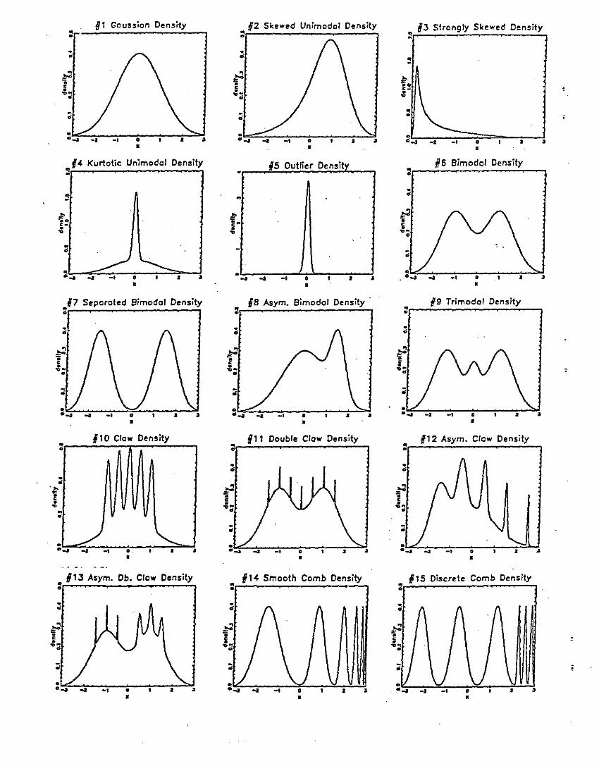
:"...;::::::..•..,.,.....-.,,-.....,.~-"!--~.,...;~.•
62 Skewed Unimodal Density:
:Io...""'::...:-.__••--•.-----;.--"=!••
#3 Strongly Skewed Density:',..::.....:.;...-...;:...:.-_-----...:..,
~••c.:•o
:l...,.--....."....::.,;::::::.;:::::=7'"--:.:--4.•
,
15 Bimodal Density•0::
..:..c•...•••· .... ... -, • • ••
19 Trimodol Density••::
..:i•...
0
:i... -. • • ••
112 Asym. Claw Density••0•
..:..c:.•••.... ... -, • • ••
liS Outlier Densitv
18 Asym. Bimodal Density':
:l~....,.:::::.....,--..,.,-~.---;--.~~.•
111 Double Claw Density::......:....,.:...:;..:...------...:--,
:'~...~~..,...--.,..--=-.-~-.....,.:-~.•
14 Kurtotic Unimodal Density::
••~ '---:,t...,,-_...=;::::::._."",--.".....-.,....::::"'.~-i..
•17 Separoted Bimodal Density
:
:,~...~-.....,.--..,......:::::.~-.,...--:.~~.•
110 Claw Density:'~--=-_....:~---=--......
./ '-::L..._c::::..::...---.--.----=.::::::~.•
o•...1
113 Asym. Db. Claw Density::
~..co...
o
.. ., •• • •
114 Smooth Comb Density:
::~..."--..----.-.::::..~--::!....~...!.!1.•
115 Discrete Comb Density••o.
f\, ./1•
..:'"• ,~...
0
:if) \) \) .\•.... -. ., • • ••
![Density-Functional Theory and Experimental Evaluation of ... · derivatives have shown corrosion inhibition properties [16,17]. Hence, the synthesis of imidazo[4,5-b]pyridine derivatives](https://img.pdfslide.net/doc/110x75/5f1a56120aa09467e934b643/density-functional-theory-and-experimental-evaluation-of-derivatives-have-shown.jpg)

![Conditional Density Estimation with Dimensionality ... · arXiv:1404.6876v1 [cs.LG] 28 Apr 2014 Conditional Density Estimation with Dimensionality Reduction via Squared-Loss Conditional](https://img.pdfslide.net/doc/110x75/5fd102c76e00d26c341eedff/conditional-density-estimation-with-dimensionality-arxiv14046876v1-cslg.jpg)