Embed Size (px)
Citation preview
Running Head: EVALUATING SIGNIFICANCE IN MIXED MODELS IN R 1
Evaluating Significance in Linear Mixed-Effects Models in R
Steven G. Luke
Brigham Young University, Department of Psychology
1001 Spencer W. Kimball Tower, Provo, Utah 84602, USA
The final publication is available at Springer via
https://doi.org/10.3758/s13428-016-0809-y

EVALUATING SIGNIFICANCE IN MIXED MODELS 2
Abstract
Mixed-effects models are being used ever more frequently in the analysis of experimental
data. However, in the lme4 package in R the standards for evaluating significance of fixed
effects in these models (i.e. obtaining p-values) are somewhat vague. There are good reasons for
this, but as researchers who are using these models are required in many cases to report p-values,
some method for evaluating the significance of the model output is needed. This paper reports
the results of simulations showing that the two most common methods for evaluating
significance, using likelihood ratio tests and applying the z distribution to the Wald t values from
the model output (t-as-z), are somewhat anti-conservative, especially for smaller sample sizes.
Other methods for evaluating significance, including parametric bootstrapping and the Kenward-
Roger and the Satterthwaite approximations for degrees of freedom, were also evaluated. The
results of these simulations suggest that Type 1 error rates are closest to .05 when models are
fitted using REML and p-values are derived using the Kenward-Roger or Satterthwaite
approximations, as these approximations both produced acceptable Type 1 error rates even for
smaller samples.

EVALUATING SIGNIFICANCE IN MIXED MODELS 3
Mixed-effects models have become increasingly popular for the analysis of experimental
data. Baayen, Davidson, and Bates (2008) provided an introduction to this method of analysis
using the lme4 package (Bates, Mächler, Bolker, & Walker, 2015b) in R (R Core Team, 2015)
that has been cited more than 1700 times as of this writing according to Web of Science. Many
researchers who attempt to transition to the use of mixed models from other analysis methods
such as ANOVAs find aspects of mixed modeling to be non-intuitive, but the one issue that has
perhaps generated the most confusion is how to evaluate the significance of the fixed effects in
the model output. This is because in lme4 the output of linear mixed models provide t-values but
no p-values. The primary motivation for this omission is that in linear mixed models it is not at
all obvious what the appropriate denominator degrees of freedom to use are, except perhaps for
some simple designs and nicely balanced data. With crossed designs or unbalanced data sets,
Baayen et al. (2008) describe the inherent uncertainty associated with counting parameters in a
model that has more than one level. They point out that for such a model, it is unclear whether
the number of observations (level 1) or the number of subjects and/or items (level 2) or the
number of grouping factors (i.e. the number of random effects), or some combination of these,
would define the denominator degrees of freedom. Although the logic behind the omission of p-
values in the R output is clear, this omission presents a problem for researchers who are
accustomed to use p-values in hypothesis testing and who are required by journals and by style
standards to report p-values.
Baayen et al. (2008) presented an elegant solution to this problem: p-values can be
estimated by using Markov-chain Monte Carlo (MCMC) sampling. This technique repeatedly
samples from the posterior distribution of the model parameters. These samples can then be used
to evaluate the probability that a given parameter is different from 0, with no degrees of freedom
EVALUATING SIGNIFICANCE IN MIXED MODELS 4
required. However, this method has significant downsides. It cannot be used when random slopes
are included in the model (or, more precisely, it was never implemented for situations when the
model included random correlation parameters). This is especially a concern given that
improperly fitted models lacking these random slopes can have catastrophically high Type 1
error rates, so that some authors recommend that all models should be “maximal”, with all
possible random slopes included (Barr, Levy, Scheepers, & Tily, 2013). Given this, it is usually
not feasible to employ MCMC sampling to obtain p-values. For this and other reasons, MCMC
sampling is no longer an option in current version of the lme4 package in R (Bates et al., 2015b).
There are two other methods commonly used for evaluating significance of fixed effects
in mixed-effects models. The first is the likelihood ratio test (LRT). LRTs compare two different
models to determine if one is a better fit to the data than the other. LRTs are commonly used to
decide if a particular parameter should be included in a mixed model. LRTs are most commonly
used to decide if a particular random effect (say, a random slope) should be retained in the model
by evaluating whether that effect improves the fit of the model, with all other model parameters
held constant. Under the right circumstances, LRTs can be used to evaluate the significance of a
particular fixed effect using the same logic. This approach shares with MCMC sampling the
advantage that the user does not need to make any specific assumptions about model degrees of
freedom (or rather, the user does not need to specify the model degrees of freedom). Further,
LRTs can be used even when the model has a complex random effects structure that includes
random slopes. When used for evaluating the significance of fixed effects, LRTs have one
potential disadvantage: Using LRTs to compare two models that differ in their fixed effects
structure may not always be appropriate (Pinheiro & Bates, 2000). When mixed-effects models
are fitted using restricted maximum likelihood (REML, the default in lme4), there is a term in the
EVALUATING SIGNIFICANCE IN MIXED MODELS 5
REML criterion that changes when the fixed-effects structure changes, making a comparison of
models differing in their fixed effects structure meaningless. Thus, if LRTs are to be used to
evaluate significance, models must be fitted using maximum likelihood (ML). Pinheiro and
Bates (2000) note that although likelihood ratio tests can be used to evaluate the significance of
fixed effects in models fitted with ML, such tests have the potential to be quite anti-conservative.
Barr et al. (2013) use this test repeatedly in their simulations, and suggest that for the numbers of
subjects and items typical of cognitive research these likelihood ratio tests are not particularly
anti-conservative. Even so, LRTs may be anti-conservative, especially for smaller data sets.
The second commonly-used method for the evaluation of significance in mixed-effects
models is to simply use the z dsitribution to obtain p-values from the Wald t-values provided by
the lme4 model output. The logic behind this t-as-z approach is that the t distribution begins to
approximate the z distribution as degrees of freedom increase, and at infinite degrees of freedom
they are identical. Given that most data sets analyzed using mixed models contain at minimum
many hundreds of data points, simply testing the Wald t-values provided in the model output as
though they were z-distributed to generate p-values is intuitively appealing. While this method is
often employed directly to generate p-values, it is also used implicitly by many authors who
refrain from presenting p-values but note that t-values greater than 1.96 can be considered
significant. There are no formalized guidelines for deciding if one’s data set is large enough to
justify the t-as-z approach. Because this assumption has not been carefully evaluated, this
technique could potentially be anti-conservative as well.
The present paper reports a series of simulations. The first set was conducted in order to
estimate the rate of Type 1 errors that arise when applying the t-as-z approach, and to compare
those rates to Type 1 error rates from LRTs. These simulations were designed to 1) explore

EVALUATING SIGNIFICANCE IN MIXED MODELS 6
whether the two commonly-used techniques for evaluating significance are anti-conservative and
2) to evaluate which method is preferable. A second set of simulations was conducted to
investigate some newer methods for evaluating significance. These methods include the
Kenward-Roger and Satterthwaite approximations for degrees of freedom, and parametric
bootstrapping. These simulations were designed to 1) compare these newer approaches to the t-
as-z approach and LRTs and 2) to evaluate which method is preferable, being least anti-
conservative and least sensitive to sample size. All simulations were run using the SIMGEN
package (Barr et al., 2013) in R to fit models to simulated data, varying number of subjects and
items systematically. R Code and results of all simulations are available on the Open Science
Framework (osf.io/fnuv4).
LRTs vs t-as-z
For each simulation, 100,000 data sets were generated from a set of population
parameters using SIMGEN, as described in Barr et al. (2013; see online appendix for code). Each
simulated experiment was designed so that the data set included a continuous response variable
and a single within-items and within-subjects two-level predictor. For the purpose of these
simulations, the size of the fixed effect was set to zero, so that any statistically significant effects
would represent Type 1 error. These simulations used the default population parameters in
SIMGEN: β0 ∼ U1(−3, 3), β1 0, τ002 ∼ U(0, 3), τ112 ∼ U(0, 3), ρS ∼ U(−.8, .8), ω002 ∼ U(0, 3), ω112
∼ U(0, 3), ρI ∼ U(−.8, .8), σ2 ∼ U(0, 3), pmissing ∼ U(.00, .05); for more information on these
parameters see Barr et al. (2013; Table 2) or the documentation for the SIMGEN package.
Simulations were performed for combinations of five different numbers of subjects (12,
24, 36, 48, 60) and five numbers of items (12, 24, 36, 48, 60), for a total of 25 different possible
1 ∼ U(min, max) means the parameter was sampled from a uniform distribution with range [min, max].

EVALUATING SIGNIFICANCE IN MIXED MODELS 7
combinations. In the first round of simulations, models were fitted using ML, and in the second
they were fitted using REML. All models were maximal, meaning that they included all possible
random intercepts and slopes2.
From each of these simulations, one or, if necessary, two slopes were dropped from the
models if the full model failed to converge (1% of cases). Type 1 error was then computed by
using the t-values provided by the models to compute p-values from the z distribution, and then
the proportion of models that were significant at the 0.05 level was calculated. For the ML
models, a similar procedure was followed to calculate Type 1 error for the LRT output as well.
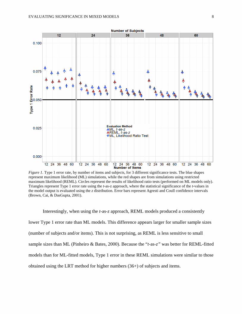
The Type 1 error rates for all simulations are shown in Figure 1. It should be apparent
from Figure 1 that all methods of evaluating significance were somewhat anti-conservative,
yielding Type 1 error rates as high as 0.08, and never at or below the 0.05 level (0.05 was never
within the 95% confidence interval for any of the simulations; see Figure 1). For models fit with
ML, the “t-as-z” method produced consistently higher error rates than the LRT method. This
difference appears greatest for smaller numbers of subjects and of items.
2 An identical set of simulations were conducted with backwards-fitted (non-maximal) models. The results of these simulations were highly similar to those reported here, in that Type 1 error rates were consistently inflated, especially for lower numbers of subjects and items, and that LRTs consistently had lower Type 1 error rates than the t-as-z approach.
EVALUATING SIGNIFICANCE IN MIXED MODELS 8
Figure 1. Type 1 error rate, by number of items and subjects, for 3 different significance tests. The blue shapes represent maximum likelihood (ML) simulations, while the red shapes are from simulations using restricted maximum likelihood (REML). Circles represent the results of likelihood ratio tests (performed on ML models only). Triangles represent Type 1 error rate using the t-as-z approach, where the statistical significance of the t-values in the model output is evaluated using the z distribution. Error bars represent Agresti and Coull confidence intervals (Brown, Cai, & DasGupta, 2001).
Interestingly, when using the t-as-z approach, REML models produced a consistently
lower Type 1 error rate than ML models. This difference appears larger for smaller sample sizes
(number of subjects and/or items). This is not surprising, as REML is less sensitive to small
sample sizes than ML (Pinheiro & Bates, 2000). Because the “t-as-z” was better for REML-fitted
models than for ML-fitted models, Type 1 error in these REML simulations were similar to those
obtained using the LRT method for higher numbers (36+) of subjects and items.
EVALUATING SIGNIFICANCE IN MIXED MODELS 9
Also of interest is the fact that in these models, which had crossed random effects for
subjects and items, Type 1 error rates vary as a function of the number of subjects and/or items
in a way that was independent of the number of data points. Note that in Figure 1 the error rates
for the simulations with 12 subjects (leftmost panel) are approximately equal for all numbers of
items. Note further that the error rate for the 24 subjects and 24 items simulations was lower than
that for the 12 subjects and 48 items simulations, even though the total number of data points
was the same in each case (24 * 24 = 576 = 12 * 48). This suggests that Type 1 error rates are
influenced by the number of second-level groups in the mixed model, and not solely determined
by the number of data points (level 1 in the model).
Discussion
The results of these simulations show that p-values calculated for linear mixed models
using either of the most frequently-used methods (LRTs, t-as-z) are somewhat anti-conservative.
Further, these p-values appear to be more anti-conservative for smaller sample sizes, although
the p-values obtained from LRTs appear to be less influenced by sample size. Type 1 error rates
were sensitive to both number of subjects and number of items together, so that higher numbers
of both were required for Type 1 error to approach acceptable levels. Further, LRTs generally
had lower Type 1 error rates across all numbers of subjects and items, making this test preferable
to the t-as-z method.
Alternate methods for evaluating significance
A number of other methods for obtaining p-values are currently available. They include
parametric bootstrapping and the Kenward-Roger and Satterthwaite approximations for degrees
of freedom3. Both the Kenward-Roger (Kenward & Roger, 1997) and Satterthwaite (1941)
3 These are the primary methods available for obtaining p-values. See the documentation for the lme4 package (Bates et al., 2015b) for options for obtaining confidence intervals.
EVALUATING SIGNIFICANCE IN MIXED MODELS 10
approaches are used to estimate denominator degrees of freedom for F statistics or degrees of
freedom for t statistics. SAS PROC MIXED uses the Satterthwaite approximation (SAS Institute,
2008). While the Satterthwaite approximation can be applied to ML or REML models, the
Kenward-Roger approximation is applied to REML models only. The significance of LRTs are
typically evaluated using a χ2 distribution, but parametric bootstrapping is an alternate method
for obtaining p-values from LRTs, in which these values are estimated by using repeated
sampling. Thus, parametric bootstrapping does not make any explicit assumptions about degrees
of freedom. As both LRTs and the t-as-z method are somewhat anti-conservative, one or more of
these methods might prove to be preferable; The Kenward-Roger approximation, for example,
appears to provide good results when applied to generalized linear mixed models (GLMMs;
Stroup, 2015). To investigate this, more simulations were conducted. The Kenward-Roger and
Satterthwaite approximations were tested together, and parametric bootstrapping was tested
separately. All simulations also included the LRT and t-as-z methods for evaluating significance.
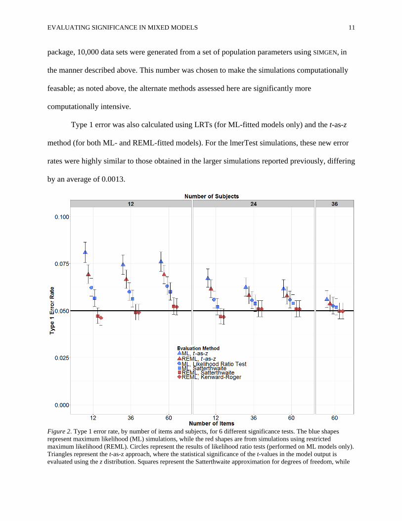
Because a primary goal of these sets of simulations was to explore Type 1 error for
smaller sample sizes, simulations were performed for combinations of 2 different numbers of
subjects (12, 24) and three numbers of items (12, 36, 60). To see how the different methods
compared for higher numbers of subjects and items, simulations with 36 subjects and 60 items
were also conducted, for a total of 7 different possible subject/item combinations.
Kenward-Roger and Satterthwaite Approximations
The Kenward-Roger and Satterthwaite approximations were implemented using the
anova function from package lmerTest (Kuznetsova, Brockhoff, & Christensen, 2014). This
function makes use of functions from the pbkrtest package (Halekoh & Højsgaard, 2014) to
implement the Kenward-Roger approximation. For each of these simulation using the lmerTest
EVALUATING SIGNIFICANCE IN MIXED MODELS 11
package, 10,000 data sets were generated from a set of population parameters using SIMGEN, in
the manner described above. This number was chosen to make the simulations computationally
feasable; as noted above, the alternate methods assessed here are significantly more
computationally intensive.
Type 1 error was also calculated using LRTs (for ML-fitted models only) and the t-as-z
method (for both ML- and REML-fitted models). For the lmerTest simulations, these new error
rates were highly similar to those obtained in the larger simulations reported previously, differing
by an average of 0.0013.
Figure 2. Type 1 error rate, by number of items and subjects, for 6 different significance tests. The blue shapes represent maximum likelihood (ML) simulations, while the red shapes are from simulations using restricted maximum likelihood (REML). Circles represent the results of likelihood ratio tests (performed on ML models only). Triangles represent the t-as-z approach, where the statistical significance of the t-values in the model output is evaluated using the z distribution. Squares represent the Satterthwaite approximation for degrees of freedom, while
EVALUATING SIGNIFICANCE IN MIXED MODELS 12
diamonds represent the Kenward-Roger approximation. Error bars represent Agresti and Coull confidence intervals (Brown et al., 2001).
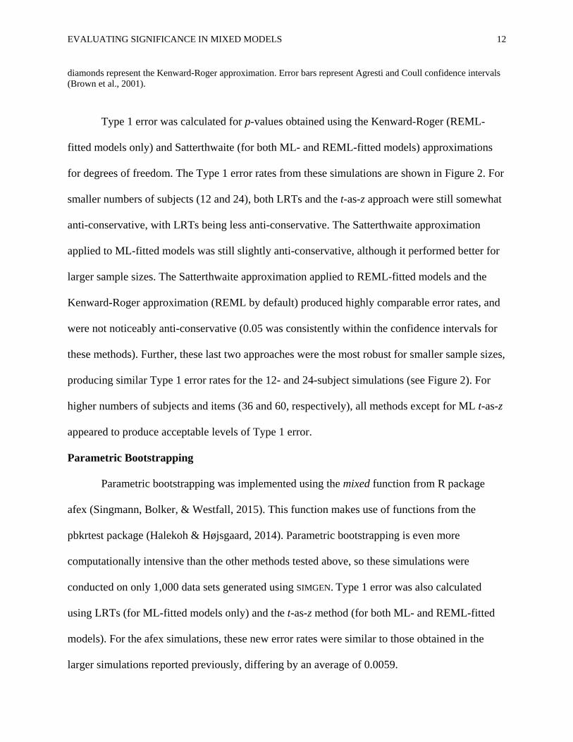
Type 1 error was calculated for p-values obtained using the Kenward-Roger (REML-
fitted models only) and Satterthwaite (for both ML- and REML-fitted models) approximations
for degrees of freedom. The Type 1 error rates from these simulations are shown in Figure 2. For
smaller numbers of subjects (12 and 24), both LRTs and the t-as-z approach were still somewhat
anti-conservative, with LRTs being less anti-conservative. The Satterthwaite approximation
applied to ML-fitted models was still slightly anti-conservative, although it performed better for
larger sample sizes. The Satterthwaite approximation applied to REML-fitted models and the
Kenward-Roger approximation (REML by default) produced highly comparable error rates, and
were not noticeably anti-conservative (0.05 was consistently within the confidence intervals for
these methods). Further, these last two approaches were the most robust for smaller sample sizes,
producing similar Type 1 error rates for the 12- and 24-subject simulations (see Figure 2). For
higher numbers of subjects and items (36 and 60, respectively), all methods except for ML t-as-z
appeared to produce acceptable levels of Type 1 error.
Parametric Bootstrapping
Parametric bootstrapping was implemented using the mixed function from R package
afex (Singmann, Bolker, & Westfall, 2015). This function makes use of functions from the
pbkrtest package (Halekoh & Højsgaard, 2014). Parametric bootstrapping is even more
computationally intensive than the other methods tested above, so these simulations were
conducted on only 1,000 data sets generated using SIMGEN. Type 1 error was also calculated
using LRTs (for ML-fitted models only) and the t-as-z method (for both ML- and REML-fitted
models). For the afex simulations, these new error rates were similar to those obtained in the
larger simulations reported previously, differing by an average of 0.0059.

EVALUATING SIGNIFICANCE IN MIXED MODELS 13
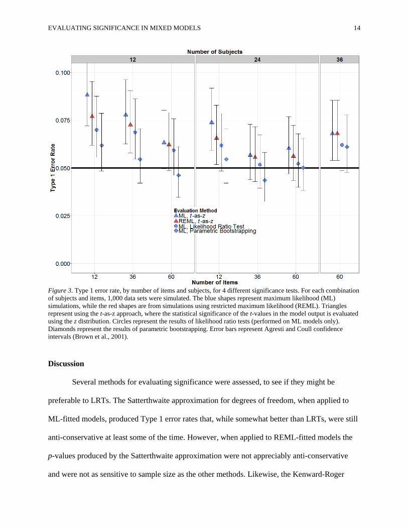
Due to the smaller number of data sets, the simulation results for parametric
bootstrapping are more variable than those for the other simulations (note the wider error bars).
Even so, it is apparent from Figure 3 that parametric bootstrapping produced lower Type 1 error
rates than LRTs and the t-as-z approach for all combinations of subjects and items when applied
to the same data sets. Indeed, Type 1 error rates for parametric bootstrapping were on average
0.0076 lower than those for LRTs from the same simulations. This is greater than the average
improvement of 0.0029 for the Satterthwaite approximation (ML models) over LRT shown in
Figure 2 and similar to the improvement observed in Figure 2 for the Kenward-Roger
approximation (0.0085 lower than LRT Type 1 error rates) and the Satterthwaite approximation
(REML models; 0.0083 lower than LRT Type 1 error rates). Figures 3 thus suggests that
parametric bootstrapping can produce acceptable error rates for all numbers of subjects/items. At
the same time, parametric bootstrapping does appear to be somewhat sensitive to sample size,
with higher error rates for smaller samples.
EVALUATING SIGNIFICANCE IN MIXED MODELS 14
Figure 3. Type 1 error rate, by number of items and subjects, for 4 different significance tests. For each combination of subjects and items, 1,000 data sets were simulated. The blue shapes represent maximum likelihood (ML) simulations, while the red shapes are from simulations using restricted maximum likelihood (REML). Triangles represent using the t-as-z approach, where the statistical significance of the t-values in the model output is evaluated using the z distribution. Circles represent the results of likelihood ratio tests (performed on ML models only). Diamonds represent the results of parametric bootstrapping. Error bars represent Agresti and Coull confidence intervals (Brown et al., 2001).
Discussion
Several methods for evaluating significance were assessed, to see if they might be
preferable to LRTs. The Satterthwaite approximation for degrees of freedom, when applied to
ML-fitted models, produced Type 1 error rates that, while somewhat better than LRTs, were still
anti-conservative at least some of the time. However, when applied to REML-fitted models the
p-values produced by the Satterthwaite approximation were not appreciably anti-conservative
and were not as sensitive to sample size as the other methods. Likewise, the Kenward-Roger
EVALUATING SIGNIFICANCE IN MIXED MODELS 15
approximation, which requires REML models, produced acceptable rates of Type 1 error, and
was also not overly sensitive to sample size. Parametric bootstrapping, as implemented here
using R package afex (Singmann et al., 2015), also produced smaller Type 1 error rates that were
superior than those obtained from LRTs and that are also likely not anti-conservative in most
cases, although parametric bootstrapping appeared to be more sensitive to sample size than the
other acceptable methods.
General Discussion
The methods most commonly used to evaluate significance in linear mixed effects
models in the lme4 package (Bates et al., 2015b) in R (R Core Team, 2015) are likelihood ratio
tests (LRTs) and the t-as-z approach, where the z distribution is used to evaluate the statistical
significance of the t-values provided in the model output. A series of simulations showed that
both of these common methods for evaluating significance are somewhat anti-conservative, with
the t-as-z approach being somewhat more so. Further, these approaches were also sensitive to
sample size, with Type 1 error rates being higher for smaller samples. At higher numbers of
subjects and items the Type 1 error rates were closer to optimal, although still slightly anti-
conservative (see Figure 1). This was true for both ML- and REML-fitted models. In Figures 2
and 3, LRTs and the t-as-z approach for REML models appear to approach acceptable levels of
Type 1 error, but the simulations represented in these Figures included fewer iterations, and so
the confidence intervals were wider. Given that these common methods tend to be anti-
conservative, and given that other, less anti-conservative methods of evaluating significance are
readily available in R, it is recommended that users be cautious in employing either of these
common methods for evaluating the significance of fixed effects, especially when numbers of
subjects or items is small (< 40-50). It is important to note that Type 1 error was sensitive to both
EVALUATING SIGNIFICANCE IN MIXED MODELS 16
the number of subjects and number of items, so that one cannot “make up for” a small number of
participants by having many items, or vice versa.
Some users replace the t-as-z approach with a rule of thumb that a t greater than 2 is to be
considered significant, in the hopes that adopting this stricter threshold will avoid the anti-
conservative bias of the t-as-z approach. Using the results of the first simulation set to explore
this t-is-2 approach reveals Type 1 error rates that are similar to LRTs, being slightly larger for
smaller numbers of subjects/items and slightly smaller for larger numbers (the actual values
depend on whether the model was fitted with ML or REML). Thus, while the t-is-2 method
appears preferable to the t-as-z approach and may be used as a rule of thumb, it is still sensitive
to sample size, being somewhat anti-conservative for smaller sample sizes.
Other methods of obtaining p-values in R were also tested, including the Satterthwaite
and Kenward-Roger approximations for degrees of freedom as well as parametric bootstrapping.
When applied to ML models, the Satterthwaite approximation was better than LRTs but still
somewhat anti-conservative. Parametric bootstrapping was also preferable to LRTs and appeared
capable of producing acceptable Type 1 error rates, although it seems that parametric
bootstrapping is still sensitive to sample size in the way that LRTs are, so that for smaller
samples parametric bootstrapping might still be anti-conservative.
The Satterthwaite and Kenward-Roger approximations produced highly comparable Type
1 error rates, at least when the Satterthwaite approximation was applied to REML models.
Neither of these methods appeared to be noticeably anti-conservative. Importantly, these
methods produced similar Type 1 error rates across different sample sizes, while error rates for
all other methods tended to increase as sample size decreased. Thus, these two methods may be
preferred when evaluating significance in mixed-effects models, especially when the number of
EVALUATING SIGNIFICANCE IN MIXED MODELS 17
subjects and/or items is smaller. Both lmerTest (Kuznetsova et al., 2014) and afex (Singmann et
al., 2015) have an anova function which can be used to provide p-values for each factor,
calculated from the F statistic. The afex function implements the Kenward-Roger approximation,
while lmerTest can be used to implement either approximation. Both functions call the
KRmodcomp function from the pbkrtest package for the Kenward-Roger approximation
(Halekoh & Højsgaard, 2014), but are somewhat simpler to use than this function. Like LRTs,
these tests provide one p-value for each factor in the model, even if a given factor has more than
one level. If the user desires parameter-specific p-values derived from the t-values in the lmer
output, the lmerTest package can provide these through the summary function using either the
Satterthwaite or Kenward-Roger approximation. Examples of the usage of these functions are
provided in the Appendix.
Several recommendations can be made based on the results of these simulations. First,
any of the alternate methods tested here are preferable to LRTs and the t-as-z approach (and its
variant, the t-as-2 approach). Second, although models fitted with maximum likelihood do not
produce catastrophically high Type 1 error rates for smaller sample sizes, REML-fitted models
still appear to be generally preferable for smaller samples. Note that the “small” samples in these
simulations still contained a minimum of 144 data points. The advantage for REML models
persisted for larger samples as well. This advantage for REML was most notable and consistent
when identical evaluation methods (t-as-z, Satterthwaite) were used. While some methods for
evaluating significance do not allow a choice between ML and REML (Kenward-Roger,
parametric bootstrapping), when the selected method for obtaining p-values permits such a
choice REML should be preferred. Third, the Kenward-Roger or Satterthwaite approximations
(applied to REML models) produced the most consistent Type 1 error rates, being neither anti-
EVALUATING SIGNIFICANCE IN MIXED MODELS 18
conservative nor overly sensitive to sample size, and so these methods may be preferable for
users who desire to avoid Type 1 error.
Users who decide to adopt either the Kenward-Roger or Satterthwaite approximations
should be aware of two potential issues. The first issue is that these recommendations are based
on simulations using somewhat idealized data and simple, single-factor models, so the observed
Type 1 error rates might not hold up for a model with a more complex covariance structure (see
Schaalje, McBride, & Fellingham, 2002, who show that the Kenward-Roger approximation,
while generally robust, can lead to inflated Type 1 error rates when complex covariance
structures were combined with small sample sizes). The second is the issue of power. The focus
of the present simulations was to identify methods that produce the most ideal Type 1 error, and
so it is possible that using the Kenward-Roger or Satterthwaite approximations could be
associated with a drop in statistical power. Given that psychology experiments are often
underpowered (Westfall, Kenny, & Judd, 2014), even a small loss of power may be a concern.
To see if there is any power loss associated with these methods, a set of small simulations (2
different numbers of subjects (12, 24) and of items (12, 24), each with 100 data sets) were
conducted with the size of the fixed effect set to 0.8 (i.e. the null hypothesis was false). The
power (defined as rate of rejection of the false null hypothesis) of all methods are shown in Table
1. The Kenward-Roger and Satterthwaite approximations (REML models) had slightly inferior
power compared to other methods across simulations. However, these methods also had lower
Type 1 error rates, so it is possible that this difference in power can be attributed to the error rate
differences. To test this, corrected power (power’) was computed, as described by Barr et al.
(2013); separate simulations were conducted, identical to those described earlier in the
paragraph, but with the null hypothesis set to true. The p-value at the 5% quantile was computed
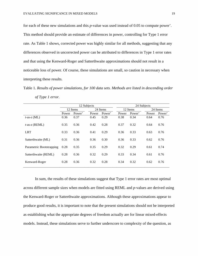
EVALUATING SIGNIFICANCE IN MIXED MODELS 19
for each of these new simulations and this p-value was used instead of 0.05 to compute power’.
This method should provide an estimate of differences in power, controlling for Type 1 error
rate. As Table 1 shows, corrected power was highly similar for all methods, suggesting that any
differences observed in uncorrected power can be attributed to differences in Type 1 error rates
and that using the Kenward-Roger and Satterthwaite approximations should not result in a
noticeable loss of power. Of course, these simulations are small, so caution in necessary when
interpreting these results.
Table 1. Results of power simulations, for 100 data sets. Methods are listed in descending order
of Type 1 error.
12 Subjects 24 Subjects 12 Items 24 Items 12 Items 24 Items
Power Power’ Power Power’ Power Power’ Power Power’ t-as-z (ML) 0.36 0.37 0.45 0.29 0.38 0.34 0.64 0.76
t-as-z (REML) 0.35 0.36 0.42 0.28 0.37 0.32 0.64 0.76
LRT 0.33 0.36 0.41 0.29 0.36 0.33 0.63 0.76
Satterthwaite (ML) 0.31 0.36 0.36 0.30 0.36 0.33 0.62 0.76
Parametric Bootstrapping 0.28 0.35 0.35 0.29 0.32 0.29 0.61 0.74
Satterthwaite (REML) 0.28 0.36 0.32 0.29 0.33 0.34 0.61 0.76
Kenward-Roger 0.28 0.36 0.32 0.28 0.34 0.32 0.62 0.76
In sum, the results of these simulations suggest that Type 1 error rates are most optimal
across different sample sizes when models are fitted using REML and p-values are derived using
the Kenward-Roger or Satterthwaite approximations. Although these approximations appear to
produce good results, it is important to note that the present simulations should not be interpreted
as establishing what the appropriate degrees of freedom actually are for linear mixed-effects
models. Instead, these simulations serve to further underscore to complexity of the question, as

EVALUATING SIGNIFICANCE IN MIXED MODELS 20
Type 1 error rates for the various tests (although quite low overall) were not predictable from
either the number of data points (level 1) or the number of grouping factors (level 2). Indeed,
methods that assume or approximate degrees of freedom in order to derive p-values for the
output of lmer models are “at best ad hoc solutions” (Bates, Mächler, Bolker, & Walker, 2015a,
p. 35). Furthermore, these simulations make it clear that results should be interpreted with
caution, regardless of the method adopted for obtaining p-values. As noted in the introduction,
there are good reasons that p-values are not included by default in lme4, and the user is
encouraged to make decisions based on an informed judgement of the parameter estimates and
their standard errors, and not to rely wholly or blindly on p-values, no matter how they were
obtained.

EVALUATING SIGNIFICANCE IN MIXED MODELS 21
References
Baayen, R. H., Davidson, D. J., & Bates, D. M. (2008). Mixed-effects modeling with crossed random effects for subjects and items. Journal of Memory and Language, 59(4), 390-412. doi: 10.1016/j.jml.2007.12.005
Barr, D. J., Levy, R., Scheepers, C., & Tily, H. J. (2013). Random effects structure for confirmatory hypothesis testing: Keep it maximal. Journal of Memory and Language, 68(3), 255-278.
Bates, D., Mächler, M., Bolker, B., & Walker, S. (2015a). Fitting Linear Mixed-Effects Models Using lme4. Journal of Statistical Software, 67(1), 1-48. doi: 10.18637/jss.v067.i01
Bates, D., Mächler, M., Bolker, B., & Walker, S. (2015b). lme4: Linear mixed-effects models using Eigen and S4. R package version 1.1-11. Retrieved from http://CRAN.R-project.org/package=lme4
Brown, L. D., Cai, T. T., & DasGupta, A. (2001). Interval Estimation for a Binomial Proportion. 101-133. doi: 10.1214/ss/1009213286
Halekoh, U., & Højsgaard, S. (2014). pbkrtest: Parametric bootstrap and Kenward Roger based methods for mixed model comparison. R package version 0.4-2.
Kenward, M. G., & Roger, J. H. (1997). Small sample inference for fixed effects from restricted maximum likelihood. Biometrics, 983-997.
Kuznetsova, A., Brockhoff, P., & Christensen, R. (2014). LmerTest: Tests for random and fixed effects for linear mixed effect models. R package, version 2.0-3.
Pinheiro, J. C., & Bates, D. M. (2000). Mixed-effects models in S and S-PLUS: Springer. R Core Team. (2015). R: A Language and Environment for Statistical Computing (Version
3.2.2). Vienna, Austria: R Foundation for Statistical Computing. Retrieved from http://www.R-project.org/
SAS Institute. (2008). SAS/STAT 9.2 user's guide Satterthwaite, F. E. (1941). Synthesis of variance. Psychometrika, 6(5), 309-316. Schaalje, G. B., McBride, J. B., & Fellingham, G. W. (2002). Adequacy of approximations to
distributions of test statistics in complex mixed linear models. Journal of Agricultural, Biological, and Environmental Statistics, 7(4), 512-524.
Singmann, H., Bolker, B., & Westfall, J. (2015). afex: Analysis of Factorial Experiments. R package, version 0.14-2.
Stroup, W. W. (2015). Rethinking the analysis of non-normal data in plant and soil science. Agronomy Journal, 107(2), 811-827.
Westfall, J., Kenny, D. A., & Judd, C. M. (2014). Statistical power and optimal design in experiments in which samples of participants respond to samples of stimuli. Journal of Experimental Psychology: General, 143(5), 2020.

EVALUATING SIGNIFICANCE IN MIXED MODELS 22
Appendix
###R Code for implementing the recommended methods for obtaining p-values in lme4.
##Using R Package lmerTest to implement Satterthwaite or Kenward-Roger approximations.
library(lmerTest) #Package must be installed first
Model.REML = lmer(Response ~ Condition + (1 + Condition | Subject) + (1 + Condition | Item), REML = TRUE,
data = MyData) #Fitting a model using REML
anova(Model.REML) #Performs F test on fixed effects using Satterthwaite approximation
anova(Model.REML, ddf = “Kenward-Roger”) #Performs F test using Kenward-Roger approximation
summary(Model.REML) #gives model output with estimated df and p values using Satterthwaite
summary(Model.REML, ddf = “Kenward-Roger”) #gives model output using Kenward-Roger
##Using Package afex to implement the Kenward-Roger approximation
library(afex) #Package must be installed first
Model.REML.afex.KR = mixed(Response ~ Condition + (1 + Condition | Subject) + (1 + Condition | Item),
data = MyData, REML = TRUE, method = “KR”) #Tests fixed effects using Kenward-Roger
Model.REML.afex.KR #Returns ANOVA table with F test on fixed effects using Kenward-Roger
Model.ML.afex.LRT = mixed(Response ~ Condition + (1 + Condition | Subject) + (1 + Condition | Item),
data = MyData, REML = FALSE, method = “LRT”) #Performs likelihood ratio tests
Model.ML.afex.LRT #Returns results of Likelihood Ration Test on Fixed Effect.
#Using LRTs is not recommended unless both number of subjects and number of items is quite large (40+)
#Note 1: This code assumes that you are attempting to obtain p-values after having settled on a final random
#effects structure. Models shown here are maximal, with all possible random slopes/intercepts.