Exact and asymptotic enumeration of perfect matchings in self-similar graphs

Discrete Mathematics 309 (2009) 6612–6625

Contents lists available at ScienceDirect

Discrete Mathematics

journal homepage: www.elsevier.com/locate/disc

Exact and asymptotic enumeration of perfect matchings inself-similar graphsElmar Teufl a, Stephan Wagner b,∗a Fakultät für Mathematik, Universität Bielefeld, P.O.Box 100131, 33501 Bielefeld, Germanyb Department of Mathematical Sciences, Stellenbosch University. Private Bag X1, Matieland 7602, South Africa

a r t i c l e i n f o

Article history:Received 24 July 2008Received in revised form 27 May 2009Accepted 8 July 2009Available online 24 July 2009

Keywords:Perfect matchingsSelf-similar graphsExact enumerationAsymptotics

a b s t r a c t

We consider self-similar graphs following a specific construction scheme: in each step,several copies of the level-n graph Xn are amalgamated to form Xn+1. Examples includefinite Sierpiński graphs or Viček graphs. For the former, the problem of counting perfectmatchings has recently been considered in a physical context by Chang and Chen[S.-C. Chang, L.-C. Chen, Dimer coverings on the Sierpiński gasket with possible vacancieson the outmost vertices, J. Statist. Phys. 131 (4) (2008) 631–650. arXiv:0711.0573v1], andwe aim to find more general results. If the number of amalgamation vertices is small or ifother conditions are satisfied, it is possible to determine explicit counting formulae forthis problem, while generally it is not even easy to obtain asymptotic information. Wealso consider the statistics ‘‘number of matching edges pointing in a given direction’’ forSierpiński graphs and show that it asymptotically follows a normal distribution. This is alsoshown inmore generality in the case that only two vertices of Xn are used for amalgamationin each step.

© 2009 Elsevier B.V. All rights reserved.

1. Introduction

The enumeration of perfect matchings belongs to the classical counting problems in graph theory. In view of itsapplications to the dimer problem in statistical physics, the enumeration of perfect matchings is particularly well-studiedfor square and hexagonal lattices—this line of investigation has been started by Kasteleyn’s fundamental work (see [5]), andthere is a vast variety of subsequent papers on the enumeration of perfectmatchings and the equivalent problemof countingdomino and lozenge tilings; Propp [7] provides a good survey of this topic. Some other papers deal with perfect matchingsin trees, cacti and other families of graphs, see for instance [3,6].Perfectmatchings of self-similar graphs have recently gained interest in the physical literature: Chang and Chen [1] study

the dimer model on the Sierpiński gasket and its higher-dimensional analogues. To be precise, they prove the followingtheorem:

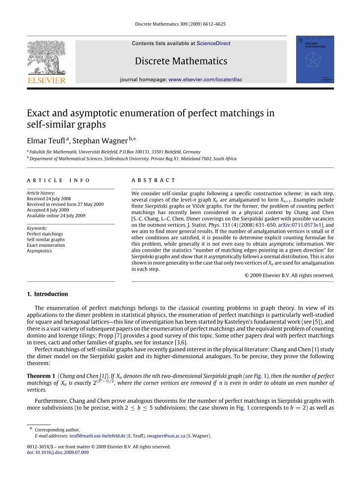
Theorem 1 (Chang and Chen [1]). If Xn denotes the nth two-dimensional Sierpiński graph (see Fig. 1), then the number of perfectmatchings of Xn is exactly 2(3

n−1)/2, where the corner vertices are removed if n is even in order to obtain an even number of

vertices.

Furthermore, Chang and Chen prove analogous theorems for the number of perfect matchings in Sierpiński graphs withmore subdivisions (to be precise, with 2 ≤ b ≤ 5 subdivisions; the case shown in Fig. 1 corresponds to b = 2) as well as

∗ Corresponding author.E-mail addresses: [email protected] (E. Teufl), [email protected] (S. Wagner).

0012-365X/$ – see front matter© 2009 Elsevier B.V. All rights reserved.doi:10.1016/j.disc.2009.07.009

http://www.elsevier.com/locate/disc

http://www.elsevier.com/locate/disc

http://arxiv.org/0711.0573v1

mailto:[email protected]

mailto:[email protected]

http://dx.doi.org/10.1016/j.disc.2009.07.009

E. Teufl, S. Wagner / Discrete Mathematics 309 (2009) 6612–6625 6613

Fig. 1. The first few finite two-dimensional Sierpiński graphs.

higher-dimensional Sierpiński graphs (dimensions 3, 4 and 5). Generally, they obtain a doubly exponential growth (i.e., thenumber of perfect matchings of the nth d-dimensional Sierpiński graph behaves like β(d+1)

nfor a certain constant β that

depends on d and the number of subdivisions). In the two-dimensional case, they even obtain exact formulae (such as theone in Theorem 1). In the higher-dimensional case, they determine numerical approximations for β with high precision.In the present paper, we aim to generalize the results obtained by Chang and Chen to a more general class of self-similar

graphs. For essentially the same class of graphs, it was shown in [8] that remarkable explicit formulae can be given for theproblem of counting spanning trees. It turns out that there are explicit formulae for the number of perfect matchings insome special cases as well, and these cases will thus be of particular interest in this paper. We consider graph sequencesX0, X1, . . . that are obtained by a recursive construction in which s copies of the graph Xn are ‘‘glued together’’ at certaindistinguished vertices (such as the corner vertices in the case of Sierpiński graphs) to obtain Xn+1. For a precise descriptionas well as several further examples, see Section 2. If the number of these distinguished vertices is either two or three, thenthere is an explicit formula for the number of perfect matchings of Xn that has the form

Cαnβsn

for certain constants C, α, β (this assumes that the number of vertices of n is even; if necessary, we remove some of thedistinguished vertices to achieve this property). If the number of distinguished vertices is four or higher, everything becomesmore intricate: this is discussed in Section 6. In certain special cases, one can still obtain explicit formulae, but in generalthe best one can hope for is the asymptotic behavior. This asymptotic analysis is carried out in detail in the case of three-dimensional Sierpiński graphs.We also consider the statistics ‘‘number of edges in a fixed direction’’ for random perfect matchings, which is particularly

natural in the aforementioned special case of the Sierpiński gasket (Theorem 1). In Section 5, we prove that this quantityhas mean 3

n+14 and variance 3

n−34 , and we also prove that it asymptotically follows a Gaussian law as n→∞.

2. Construction

Let us now define what exactly we mean by self-similar graphs: we construct them by a recursive process that buildsa graph Y by amalgamating several copies of a graph X . Iterating this process, we obtain a sequence of graphs. In orderto formally define the graph sequences we are going to investigate, the following essential ingredients are needed (cf. theconstruction in [9,8]):

• For a given (multi)graph X , fix θ ≥ 2 distinguished vertices by an injective map ϕ : Θ → VX , where Θ = {1, . . . , θ}.These vertices are needed for the amalgamation.• Take s ≥ 2 mutually disjoint isomorphic copies Z1, Z2, . . . , Zs of X . We denote the isomorphism between X and Zi byζi : VX → VZi.• Now we have to describe how these copies are glued together to form a single graph. To this end, consider a set Gof vertices (disjoint from VZ1, . . . , VZs), and define s injective maps σi : Θ → G for i ∈ S = {1, . . . , s} such thatG =

⋃si=1 σi(Θ). The map σi defines vertices that will be identified with the distinguished vertices of Zi. Formally, let

Z be the disjoint union of Z1, . . . , Zs and G (G is regarded as an edgeless graph), and define the relation ∼ on VZ as thereflexive, symmetric, and transitive hull of

s⋃i=0

{(σi(k), ζi(ϕ(k))) : k ∈ Θ} ⊆ VZ × VZ .

Now we define a new multigraph Y by its vertex set VY = VZ/∼ and edge (multi-)set

EY = {{[v], [w]} : {v,w} ∈ EZ} ,

where [v] denotes the equivalence class of a vertex v. In words, Y is the amalgamation of Z1, Z2, . . . , Zs, wheredistinguished vertices ζi(ϕ(k)) and ζj(ϕ(`)) of two distinct copies Zi and Zj are amalgamated if (and only if) σi(k) = σj(`).The condition that G =

⋃si=1 σi(Θ) guarantees that there are no ‘‘leftover’’ vertices in G: every vertex of G is identified

with at least one vertex of the disjoint union⋃si=1 Zi. This also implies that Y does not contain isolated vertices if this is

also the case for X .• Finally, we need to define distinguished vertices on Y in order to repeat the process: to this end, let η : Θ → G be aninjective map, and define distinguished vertices on Y by amapψ : Θ → VY as follows:ψ(i) = [η(i)] ∈ VY for all i ∈ Θ .

6614 E. Teufl, S. Wagner / Discrete Mathematics 309 (2009) 6612–6625

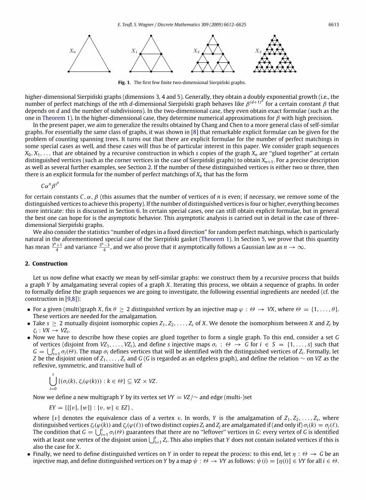
Fig. 2. An example of a sequence of finite self-similar graphs.

If we fix G, η, and {σi : i ∈ S}, we obtain a procedure that constructs a multigraph Y together with distinguished vertices(given by an injective map ψ : Θ → VY ) from any multigraph X and any injective map ϕ : Θ → VX . If the pair (Y , ψ) isconstructed from (X, ϕ) in this way, write (Y , ψ) = Copy(X, ϕ). Since G, η, and {σi : i ∈ S} are fixed, the dependence onthese items is suppressed. For i ∈ S, define Z̄i by

V Z̄i = {[v] : v ∈ VZi} and EZ̄i = {{[v], [w]} : {v,w} ∈ EZi} .

Then Z̄i is isomorphic to X and the isomorphism is given by

ζ̄i : VX → V Z̄i, v 7→ [ζi(v)].

The subgraph Z̄i is called the i-th part of Y . On the ith part of Y distinguished vertices are given by

Θ → V Z̄i, k 7→ ζ̄i(ϕ(k)) = [σi(k)].

In the following, we will be interested in sequences of graphs obtained by iterating this construction, i.e., X0 is someinitial graph with distinguished vertices given by a map ϕ0, and (Xn, ϕn) = Copy(Xn−1, ϕn−1). The graphs X0, X1, X2, . . .constructed in this manner are called a sequence of (finite) self-similar graphs.We will also need some symmetry condition in the following sections: it will be assumed that the graphs Xn are strongly

symmetric with respect to ϕn(Θ), which means that the automorphism group of Xn acts like the alternating group or thesymmetric group on ϕn(Θ), with one exception: if θ = 2 we assume that the action is given by the symmetric group. If thiscondition is satisfied, then we have the following simple yet important property:

Lemma 2. For any two subsets M1,M2 ⊆ Θ with |M1| = |M2| and any non-negative integer n, there is an automorphism π ofXn such that π(ϕn(M1)) = ϕn(M2).

2.1. Examples

In this subsection we present some examples of self-similar graphs illustrating the construction. Note that all examplessatisfy the symmetry condition.

2.1.1. An example with two distinguished verticesLet θ = 2 and s = 6 and set G = {1, 2, 3, 4, 5, 6}. Furthermore, define the maps η and σj by the following table:

i η(i) σ1(i) σ2(i) σ3(i) σ4(i) σ5(i) σ6(i)

1 1 1 2 2 3 4 52 6 2 3 5 4 5 6

With these definitions we build a sequence of finite self-similar graphs Xn by setting X0 = K2 (ϕ0 can be either of the twobijections between {1, 2} and the two vertices of the complete graph K2) and (Xn, ϕn) = Copy(Xn−1, ϕn−1) (Fig. 2).

2.1.2. Finite Sierpiński graphsSierpiński graphs have already been mentioned in the introduction. Let us show how they can be obtained by means of

our construction. Fix some d ∈ N (the dimension), and let s = θ = d+ 1. Define G by

G ={x ∈ Nd+10 : x1 + x2 + · · · + xd+1 = 2

}and the map η : Θ → G by η(i) = 2ei, where ei is the ith canonical basis vector of Rd+1. In addition, set σi(j) = ei + ej ∈ Gfor i ∈ S and j ∈ Θ (note that Θ = S = {1, . . . , d + 1}). It is easy to see that |G| = 1

2 (d + 2)(d + 1). The usual finited-dimensional Sierpiński graphs are then obtained by setting X0 = Kθ (again, ϕ0 can be any bijection betweenΘ and the θvertices of the complete graph Kθ ) and iterating (Xn, ϕn) = Copy(Xn−1, ϕn−1) for n ∈ N. See Fig. 1 for the case d = 2.


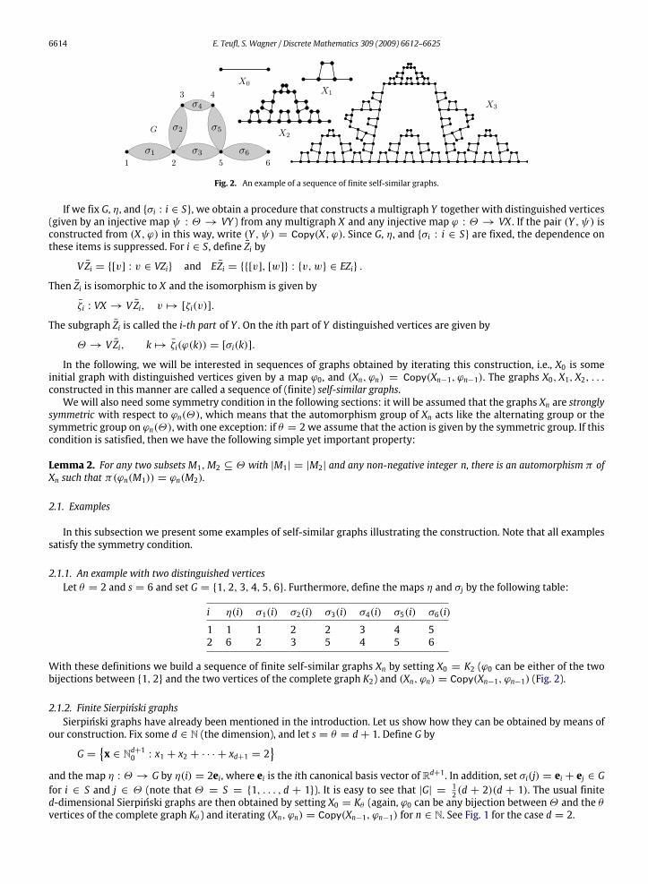
Fig. 3. The first few finite Viček graphs.

2.1.3. Finite Viček graphsFix some integer θ ≥ 2 and set s = θ + 1. Recall thatΘ = {1, 2, . . . , θ} and define G = Θ ×Θ . Then define the maps η

and σi by η(i) = (i, 1) and

σi(j) ={(i, j) if i ∈ Θ,(j, 2) if i = s = θ + 1.

With this data the finite Viček graphs are defined as follows: the initial graph X0 is the complete graph Kθ (ϕ0 is trivial onceagain), and Xn is defined by (Xn, ϕn) = Copy(Xn−1, ϕn−1), as always. Fig. 3 shows the first few Viček graphs for θ = 4.

3. Perfect matchings

A matching is a set of disjoint edges of a graph, a perfect matching is a matching which covers all vertices of a graph. Leta graph X with θ distinguished vertices (defined by an injective map ϕ : Θ → VX , as in the previous section) be given suchthat X is strongly symmetric with respect to ϕ(Θ). We denote the set of matchings byM(X) and defineMK (X) to be the setof all perfect matchings of X \ ϕ(K) for any set K ⊆ Θ . Then, in view of strong symmetry, the size ofMK (X) only dependson the cardinality of K , and we may define mk(X) = |MK (X)| for any set K of cardinality |K | = k. Note that mk(X) = 0 ifk 6≡ |VX | mod 2.Now, if Y = Copy(X), wewant to express the values ofmk(Y ) in terms of themj(X). To this end, note that everymatching

M inMK (Y ) inducesmatchings on all parts Z̄i of Y . For each i, letMi be the restriction ofM to the ith part Z̄i:Mi = M∩EZ̄i. Thematching Mi has to cover all vertices of Z̄i except possibly some of the distinguished vertices of Z̄i. Hence ζ̄−1i (Mi) belongstoMLi(X) for some set Li. Moreover, for each v ∈ G \ η(K), there is exactly one i = ρ(v) such that the vertex [v] ∈ VY iscovered by an edge in the part Z̄i.Conversely, using the same set K , define a map ρ : G \ η(K)→ S such that v ∈ σρ(v)(Θ) for all v, and choose a perfect

matchingMi in X \ϕ(Θ \σ−1i (ρ−1(i))) for each i ∈ S (i.e., in the preimage of Z̄i, reduced by all vertices which are not coveredwithin Z̄i), if possible. Then

⋃si=1 ζ̄i(Mi) is a matching inMK (Y ). So we have established a bijective correspondence between

MK (Y ) and all possible tuples (ρ,M1, . . . ,Ms). Here, Mi is a matching in MLi for some set Li of cardinality θ − |ρ−1(i)|.

Hence, the formula

mk(Y ) =∑ρ

s∏i=1

mθ−|ρ−1(i)|(X) (1)

holds, where the sum is over all possible functions ρ which satisfy the above condition, and K is an arbitrary set of size k.The following simple lemma is an immediate consequence:

Lemma 3. For every 0 ≤ k ≤ θ , there exist non-negative integer coefficients a(k, ν) such that

mk(Y ) =∑

ν

a(k, ν)θ∏j=0

mj(X)νj ,

where the sum is over all (θ + 1)-tuples ν = (ν0, . . . , νθ ) of non-negative integers such thatθ∑j=0

νj = s andθ∑j=0

jνj = sθ − |G| + k.

Proof. We only have to check that in Eq. (1), the identitys∑i=1

(θ − |ρ−1(i)|) = sθ − |G| + k


holds. Then the lemma follows easily from Eq. (1). However, this is equivalent to

|dom(ρ)| =s∑i=1

|ρ−1(i)| = |G| − k,

which is obviously true (dom(ρ) denotes the domain of ρ). �

If one wants to determine the coefficients a(k, ν) for a specific example, one can proceed as follows: for any k, choose aset K of cardinality k as above, and consider, for any v ∈ G\η(K), the set I(v) = {i : v ∈ σi(Θ)}. A function ρ : G\η(K)→ Ssatisfies the above condition if and only if ρ(v) ∈ I(v) for all v. Now construct all

∏v∈G\η(K) |I(v)| such functions, and de-

termine θ − |ρ−1(i)| (for all i ∈ S) for each of these functions. Use these values in Eq. (1), and expand the polynomial onthe right-hand side. This might become tedious for large examples if one is working by hand, but can be done in a simplebrute-force manner by means of a computer.In the following, some examples for the resulting recurrences are provided and analyzed. The special cases θ = 2 and

θ = 3 have particularly nice properties yielding explicit formulae, and so we are going to deal with them first.Note that the number of vertices in Xn satisfies a first-order linear recurrence, namely

|VXn| = s|VXn−1| + |G| − sθ.

Hence there are three possibilities, depending on s and δ = sθ − |G|:

• |VXn| is even for all n > 0, so that mk(Xn) can only be positive if k is even. This happens if s and δ are both even or if s isodd and δ, |VX0| are even.• |VXn| is odd for all n > 0, so that mk(Xn) can only be positive if k is odd. This happens if s is even and δ odd or if s, |VX0|are odd and δ even.• |VXn| is alternately odd and even, andmk(Xn) behaves accordingly. This happens if s, δ are both odd.

4. The special cases of two or three distinguished vertices

In the cases θ = 2 and θ = 3 it is possible to derive exact formulae for the quantitiesmk(Xn), as will be exhibited in thissection. Specifically, we have the following theorem:

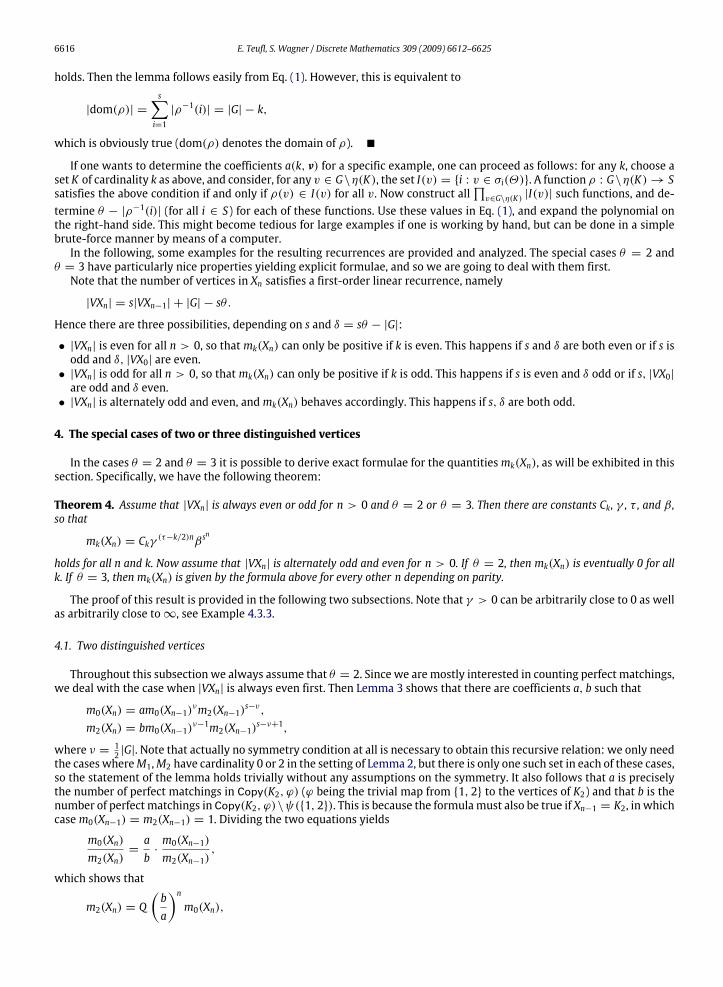
Theorem 4. Assume that |VXn| is always even or odd for n > 0 and θ = 2 or θ = 3. Then there are constants Ck, γ , τ , and β ,so that

mk(Xn) = Ckγ (τ−k/2)nβsn

holds for all n and k. Now assume that |VXn| is alternately odd and even for n > 0. If θ = 2, then mk(Xn) is eventually 0 for allk. If θ = 3, then mk(Xn) is given by the formula above for every other n depending on parity.

The proof of this result is provided in the following two subsections. Note that γ > 0 can be arbitrarily close to 0 as wellas arbitrarily close to∞, see Example 4.3.3.

4.1. Two distinguished vertices

Throughout this subsection we always assume that θ = 2. Since we are mostly interested in counting perfect matchings,we deal with the case when |VXn| is always even first. Then Lemma 3 shows that there are coefficients a, b such that

m0(Xn) = am0(Xn−1)νm2(Xn−1)s−ν,m2(Xn) = bm0(Xn−1)ν−1m2(Xn−1)s−ν+1,

where ν = 12 |G|. Note that actually no symmetry condition at all is necessary to obtain this recursive relation: we only need

the cases whereM1,M2 have cardinality 0 or 2 in the setting of Lemma 2, but there is only one such set in each of these cases,so the statement of the lemma holds trivially without any assumptions on the symmetry. It also follows that a is preciselythe number of perfect matchings in Copy(K2, ϕ) (ϕ being the trivial map from {1, 2} to the vertices of K2) and that b is thenumber of perfect matchings in Copy(K2, ϕ)\ψ({1, 2}). This is because the formulamust also be true if Xn−1 = K2, in whichcasem0(Xn−1) = m2(Xn−1) = 1. Dividing the two equations yields

m0(Xn)m2(Xn)

=ab·m0(Xn−1)m2(Xn−1)

,

which shows that

m2(Xn) = Q(ba

)nm0(Xn),


where Q = m2(X0)m0(X0)

. We use this in the formula form0(Xn) to obtain

m0(Xn) = aQ s−ν(ba

)(s−ν)(n−1)m0(Xn−1)s

with the explicit solution

m0(Xn) = C0γ τnβsn, m2(Xn) = C2γ (τ−1)nβs

n,

where the constants C0,C2,γ ,τ , and β are given as follows:

γ =ab, τ =

s− νs− 1

, C0 = (a−1γ τ )1/(s−1)Q−τ ,

C2 = C0Q , β = C−10 m0(X0).

The case when |VXn| is always odd is less interesting. We already know thatm0(Xn) = m2(Xn) = 0 for all n > 0. In viewof Lemma 3, m1(Xn) = 0 holds as well for almost all n unless |G| = s + 1 (otherwise, there is no solution to ν1 = s andν1 = 2s− |G| + 1). Then, however, there exists a constant a so thatm1(Xn) = am1(Xn−1)s with the simple solution

m1(Xn) = a11−s ·

(m1(X0)a

1s−1

)sn.

Finally, we consider the casewhen the parity of |VXn| is alternating. In this case, the quantitiesm0(Xn),m1(Xn), andm2(Xn)are equal to 0 for almost all n, which can be shown by similar arguments: first, note that eitherm0(Xn) orm2(Xn) has to be 0for almost all n by Lemma 3 (there cannot exist solutions to the systems ν1 = s, ν1 = 2s− |G| and ν1 = s, ν1 = 2s− |G| + 2simultaneously). Thus, suppose for instance that m2(Xn) = 0 for almost all n and that |G| = s (so that there exists ν1 withν1 = s = 2s−|G|). But thenm1(Xn) = 0 for almost all n, as there is no solution to the system ν0 = s, 0 = 2s−|G|+1 = s+1.The second case is treated similarly.

4.2. Three distinguished vertices

Now we assume that θ = 3 and obtain similar results as in the previous subsection. First, let us consider the case when|VXn| is always even again. Then we have

m0(Xn) = am0(Xn−1)νm2(Xn−1)s−ν,m2(Xn) = bm0(Xn−1)ν−1m2(Xn−1)s−ν+1

for some integer coefficients a, b, where ν = 12 (|G| − s). In order to determine the precise values of a and b in specific

examples, use the algorithm that is described after Lemma 3. Note that this system of recurrences is basically the same asin the case θ = 2.The case when |VXn| is always odd is also completely analogous. We obtain a system

m1(Xn) = am1(Xn−1)νm3(Xn−1)s−ν,m3(Xn) = bm1(Xn−1)ν−1m3(Xn−1)s−ν+1,

where ν = 12 (|G| − 1). The solution follows again along the same lines.

Finally, let us consider the case when the parity of |VXn| is alternating. Then we obtain the system

m0(Xn) = a0m1(Xn−1)νm3(Xn−1)s−ν,m1(Xn) = a1m0(Xn−1)κm2(Xn−1)s−κ ,m2(Xn) = a2m1(Xn−1)ν−1m3(Xn−1)s−ν+1,m3(Xn) = a3m0(Xn−1)κ−1m2(Xn−1)s−κ+1

for certain integers a0, a1, a2, a3, where ν = 12 |G| and κ =

12 (|G| − s− 1). We iterate this system once to obtain

m0(Xn) = c0m0(Xn−2)λm2(Xn−2)s2−λ,

m2(Xn) = c2m0(Xn−2)λ−1m2(Xn−2)s2−λ+1

for integer coefficients c0, c2 and λ = ν + (κ − 1)s = 12

((s+ 1)|G| − s2 − 3s

). Again, this system can be solved as in

Section 4.1.

4.3. Examples

Let us now apply Theorem 4 to the examples of Section 2.1.


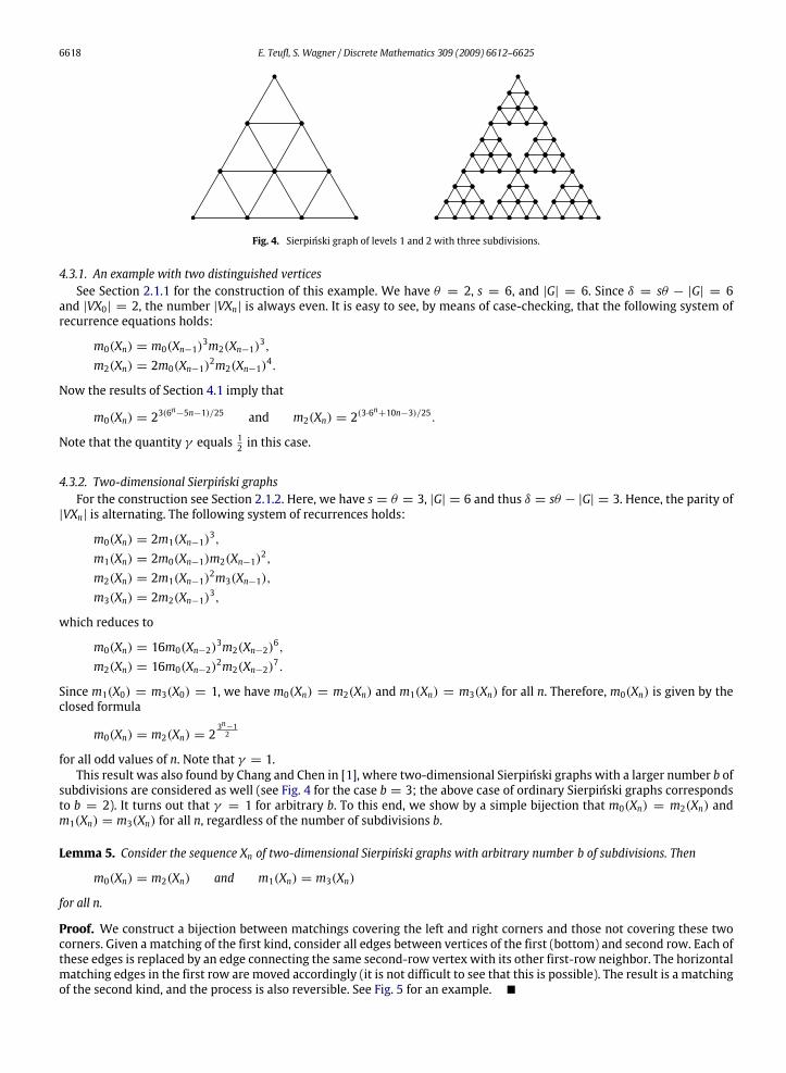
Fig. 4. Sierpiński graph of levels 1 and 2 with three subdivisions.

4.3.1. An example with two distinguished verticesSee Section 2.1.1 for the construction of this example. We have θ = 2, s = 6, and |G| = 6. Since δ = sθ − |G| = 6

and |VX0| = 2, the number |VXn| is always even. It is easy to see, by means of case-checking, that the following system ofrecurrence equations holds:

m0(Xn) = m0(Xn−1)3m2(Xn−1)3,m2(Xn) = 2m0(Xn−1)2m2(Xn−1)4.

Now the results of Section 4.1 imply that

m0(Xn) = 23(6n−5n−1)/25 and m2(Xn) = 2(3·6

n+10n−3)/25.

Note that the quantity γ equals 12 in this case.

4.3.2. Two-dimensional Sierpiński graphsFor the construction see Section 2.1.2. Here, we have s = θ = 3, |G| = 6 and thus δ = sθ − |G| = 3. Hence, the parity of

|VXn| is alternating. The following system of recurrences holds:

m0(Xn) = 2m1(Xn−1)3,m1(Xn) = 2m0(Xn−1)m2(Xn−1)2,m2(Xn) = 2m1(Xn−1)2m3(Xn−1),m3(Xn) = 2m2(Xn−1)3,

which reduces to

m0(Xn) = 16m0(Xn−2)3m2(Xn−2)6,m2(Xn) = 16m0(Xn−2)2m2(Xn−2)7.

Since m1(X0) = m3(X0) = 1, we have m0(Xn) = m2(Xn) and m1(Xn) = m3(Xn) for all n. Therefore, m0(Xn) is given by theclosed formula

m0(Xn) = m2(Xn) = 23n−12

for all odd values of n. Note that γ = 1.This result was also found by Chang and Chen in [1], where two-dimensional Sierpiński graphs with a larger number b of

subdivisions are considered as well (see Fig. 4 for the case b = 3; the above case of ordinary Sierpiński graphs correspondsto b = 2). It turns out that γ = 1 for arbitrary b. To this end, we show by a simple bijection that m0(Xn) = m2(Xn) andm1(Xn) = m3(Xn) for all n, regardless of the number of subdivisions b.

Lemma 5. Consider the sequence Xn of two-dimensional Sierpiński graphs with arbitrary number b of subdivisions. Then

m0(Xn) = m2(Xn) and m1(Xn) = m3(Xn)

for all n.

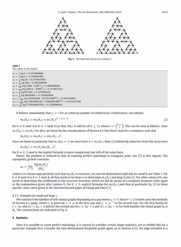
Proof. We construct a bijection between matchings covering the left and right corners and those not covering these twocorners. Given a matching of the first kind, consider all edges between vertices of the first (bottom) and second row. Each ofthese edges is replaced by an edge connecting the same second-row vertex with its other first-row neighbor. The horizontalmatching edges in the first row are moved accordingly (it is not difficult to see that this is possible). The result is a matchingof the second kind, and the process is also reversible. See Fig. 5 for an example. �


Fig. 5. The bijection that proves Lemma 5.

Table 1The values αb for small b.

α2 =13 log 2 = 0.2310490602

α3 =17 log 6 = 0.2559656385

α4 =112 log 28 = 0.2776837092

α5 =118 log 200 = 0.2943509648

α6 =1550 log

(1386 · 219621

)= 0.3069389564

α7 =1924 log

(16814 · 3700427

)= 0.3178972533

α8 =142 log 957304 = 0.3279018162

α9 =152 log 38016960 = 0.3356450564

α10 =13528 log

(220240306 · 231763140055

)= 0.3416156081

α11 =14950 log

(10032960146 · 21689368180065

)= 0.3474147262

α12 =188 log 31159166587056 = 0.3530696544

It follows immediately that γ = 1 for an arbitrary number of subdivisions. Furthermore, one obtains

m1(Xn) = m3(Xn) = m1(X1)(sn−1)/(s−1) (2)

for b ≡ 0 mod 4 or b ≡ 1 mod 4 (so that |VXn| is odd for all n ≥ 1), where s =(b+12

). This can be seen as follows: since

m1(Xn) = m3(Xn) for all n, we know by the considerations of Section 4.2 that there must be a constant a such that

m1(Xn) = m3(Xn) = am1(Xn−1)s.

Since we know in particular thatm1(X0) = 1, we must have a = m1(X1). Now (2) follows by induction from the recurrence

m1(Xn) = m1(X1)m1(Xn−1)s.

For b ≡ 2, 3 mod 4, the explicit formula is more complicated, but still of the same form.Hence, the problem is reduced to that of counting perfect matchings in triangular grids (see [7] in this regard). The

asymptotic growth constants

αb = limn→∞

logmk(Xn)|VXn|

(where k is chosen appropriately such thatmk(Xn) is nonzero) can now be determined explicitly for small b, see Table 1. Forb ≡ 0 mod 4 or b ≡ 1 mod 4, all that needs to be done is to determinem1(X1) and plug it into (2). For other values of b, oneneeds to determine the coefficients in the recursive formulae, which we did by means of a computer program (refer againto the explanations given after Lemma 3). For b ≤ 5, explicit formulae for mk(Xn) (and thus in particular Eq. (2) in thesespecific cases) were given in the aforementioned paper of Chang and Chen [1].

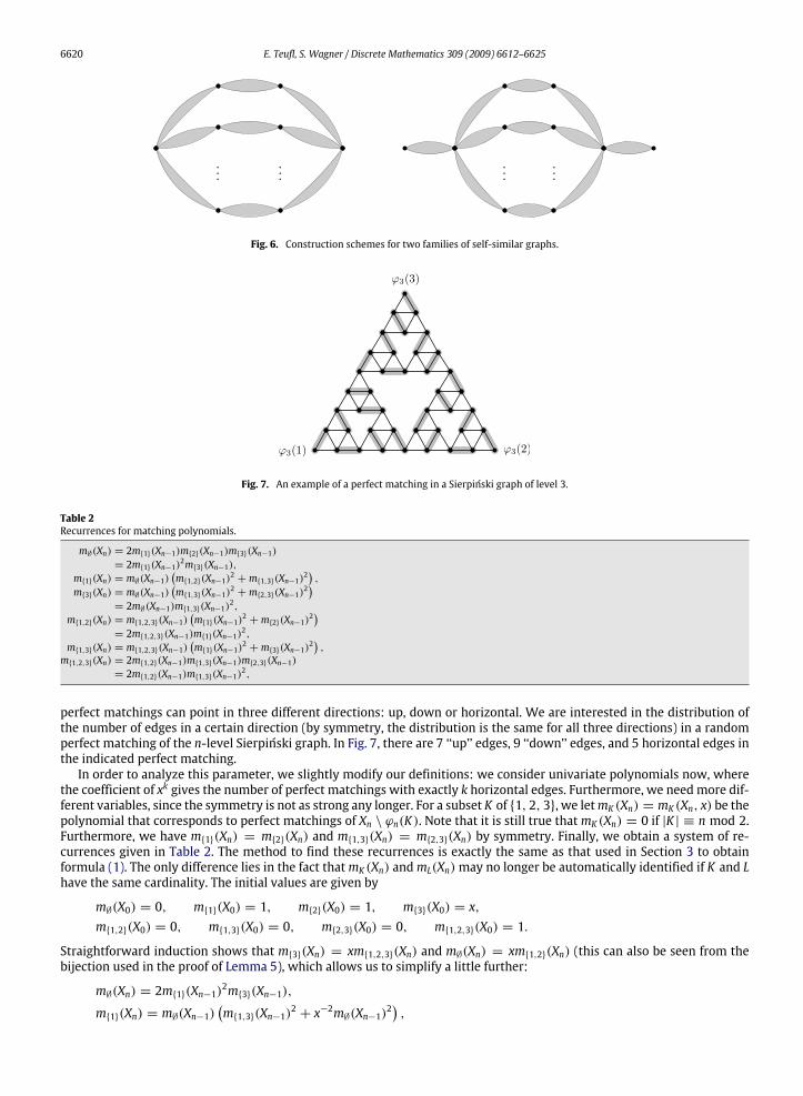
4.3.3. Examples for small and large γWe construct two families of self-similar graphs depending on a parameterµ ∈ N. Since θ = 2 in both cases themethods

of Section 4.1 apply, where γ is given by γ = µ in the first case and γ = µ−1 in the second case. For the first family lets = 3µ and |G| = 2µ+ 2 and for the second one let s = 3µ+ 2 and |G| = 2µ+ 4. For both families the initial graph X0 isK2. The constructions are indicated in Fig. 6.

5. Statistics

Once it is possible to count perfect matchings, it is natural to consider certain shape statistics. Let us exhibit this for aparticular example first. Consider the two-dimensional Sierpiński graph again, as in Section 4.3.2. An edge included in a


Fig. 6. Construction schemes for two families of self-similar graphs.

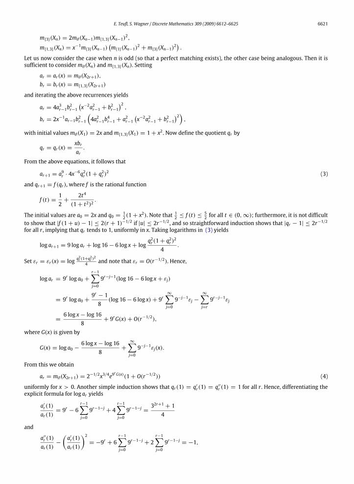
Fig. 7. An example of a perfect matching in a Sierpiński graph of level 3.

Table 2Recurrences for matching polynomials.

m∅(Xn) = 2m{1}(Xn−1)m{2}(Xn−1)m{3}(Xn−1)= 2m{1}(Xn−1)2m{3}(Xn−1),

m{1}(Xn) = m∅(Xn−1)(m{1,2}(Xn−1)2 +m{1,3}(Xn−1)2

),

m{3}(Xn) = m∅(Xn−1)(m{1,3}(Xn−1)2 +m{2,3}(Xn−1)2

)= 2m∅(Xn−1)m{1,3}(Xn−1)2,

m{1,2}(Xn) = m{1,2,3}(Xn−1)(m{1}(Xn−1)2 +m{2}(Xn−1)2

)= 2m{1,2,3}(Xn−1)m{1}(Xn−1)2,

m{1,3}(Xn) = m{1,2,3}(Xn−1)(m{1}(Xn−1)2 +m{3}(Xn−1)2

),

m{1,2,3}(Xn) = 2m{1,2}(Xn−1)m{1,3}(Xn−1)m{2,3}(Xn−1)= 2m{1,2}(Xn−1)m{1,3}(Xn−1)2,

perfect matchings can point in three different directions: up, down or horizontal. We are interested in the distribution ofthe number of edges in a certain direction (by symmetry, the distribution is the same for all three directions) in a randomperfect matching of the n-level Sierpiński graph. In Fig. 7, there are 7 ‘‘up’’ edges, 9 ‘‘down’’ edges, and 5 horizontal edges inthe indicated perfect matching.In order to analyze this parameter, we slightly modify our definitions: we consider univariate polynomials now, where

the coefficient of xk gives the number of perfect matchings with exactly k horizontal edges. Furthermore, we need more dif-ferent variables, since the symmetry is not as strong any longer. For a subset K of {1, 2, 3}, we letmK (Xn) = mK (Xn, x) be thepolynomial that corresponds to perfect matchings of Xn \ ϕn(K). Note that it is still true thatmK (Xn) = 0 if |K | ≡ n mod 2.Furthermore, we have m{1}(Xn) = m{2}(Xn) and m{1,3}(Xn) = m{2,3}(Xn) by symmetry. Finally, we obtain a system of re-currences given in Table 2. The method to find these recurrences is exactly the same as that used in Section 3 to obtainformula (1). The only difference lies in the fact thatmK (Xn) andmL(Xn)may no longer be automatically identified if K and Lhave the same cardinality. The initial values are given by

m∅(X0) = 0, m{1}(X0) = 1, m{2}(X0) = 1, m{3}(X0) = x,m{1,2}(X0) = 0, m{1,3}(X0) = 0, m{2,3}(X0) = 0, m{1,2,3}(X0) = 1.

Straightforward induction shows that m{3}(Xn) = xm{1,2,3}(Xn) and m∅(Xn) = xm{1,2}(Xn) (this can also be seen from thebijection used in the proof of Lemma 5), which allows us to simplify a little further:

m∅(Xn) = 2m{1}(Xn−1)2m{3}(Xn−1),

m{1}(Xn) = m∅(Xn−1)(m{1,3}(Xn−1)2 + x−2m∅(Xn−1)2

),


m{3}(Xn) = 2m∅(Xn−1)m{1,3}(Xn−1)2,

m{1,3}(Xn) = x−1m{3}(Xn−1)(m{1}(Xn−1)2 +m{3}(Xn−1)2

).

Let us now consider the case when n is odd (so that a perfect matching exists), the other case being analogous. Then it issufficient to considerm∅(Xn) andm{1,3}(Xn). Setting

ar = ar(x) = m∅(X2r+1),br = br(x) = m{1,3}(X2r+1)

and iterating the above recurrences yields

ar = 4a3r−1b2r−1

(x−2a2r−1 + b

2r−1

)2,

br = 2x−1ar−1b2r−1(4a2r−1b

4r−1 + a

2r−1

(x−2a2r−1 + b

2r−1

)2),

with initial valuesm∅(X1) = 2x andm{1,3}(X1) = 1+ x2. Now define the quotient qr by

qr = qr(x) =xbrar.

From the above equations, it follows that

ar+1 = a9r · 4x−6q2r (1+ q

2r )2 (3)

and qr+1 = f (qr), where f is the rational function

f (t) =12+

2t4

(1+ t2)2.

The initial values are a0 = 2x and q0 = 12 (1+ x

2). Note that 12 ≤ f (t) ≤52 for all t ∈ (0,∞); furthermore, it is not difficult

to show that |f (1+ u)− 1| ≤ 2(r + 1)−1/2 if |u| ≤ 2r−1/2, and so straightforward induction shows that |qr − 1| ≤ 2r−1/2for all r , implying that qr tends to 1, uniformly in x. Taking logarithms in (3) yields

log ar+1 = 9 log ar + log 16− 6 log x+ logq2r (1+ q

2r )2

4.

Set εr = εr(x) = logq2r (1+q

2r )2

4 and note that εr = O(r−1/2). Hence,

log ar = 9r log a0 +r−1∑j=0

9r−j−1(log 16− 6 log x+ εj)

= 9r log a0 +9r − 18

(log 16− 6 log x)+ 9r∞∑j=0

9−j−1εj −∞∑j=r

9r−j−1εj

=6 log x− log 16

8+ 9rG(x)+ O(r−1/2),

where G(x) is given by

G(x) = log a0 −6 log x− log 16

8+

∞∑j=0

9−j−1εj(x).

From this we obtain

ar = m∅(X2r+1) = 2−1/2x3/4e9rG(x)(1+ O(r−1/2)) (4)

uniformly for x > 0. Another simple induction shows that qr(1) = q′r(1) = q′′r (1) = 1 for all r . Hence, differentiating the

explicit formula for log ar yields

a′r(1)ar(1)

= 9r − 6r−1∑j=0

9r−1−j + 4r−1∑j=0

9r−1−j =32r+1 + 14

and

a′′r (1)ar(1)

−

(a′r(1)ar(1)

)2= −9r + 6

r−1∑j=0

9r−1−j + 2r−1∑j=0

9r−1−j = −1,


which implies that the mean of the number of horizontal edges is exactly

a′r(1)ar(1)

=32r+1 + 14

(one third of the total number of edges in a perfect matching, as it was to be expected), while the variance is

a′′r (1)ar(1)

+a′r(1)ar(1)

−

(a′r(1)ar(1)

)2=32r+1 − 34

.

In the same way, one finds G′(1) = 34 and G

′′(1) = 0. Finally, let Hr denote the number of horizontal edges in a randomperfect matching of X2r+1, and consider the normalized random variable

Nr =Hr − µrσr

, where µr =32r+1 + 14

and σ 2r =32r+1 − 34

.

Its moment generating function is given by

E(etNr ) = e−µr t/σrE(etHr /σr ) = e−µr t/σrar(et/σr

)ar(1)

.

Making use of the asymptotic formula (4), we obtain

E(etNr

)= exp

(−µr tσr+3t4σr+ 9r

(G(et/σr )− G(1)

))(1+ O(r−1/2))

= exp(−µr tσr+3t4σr+ 9r

(G′(1)

tσr+ G′(1)

t2

2σ 2r+ G′′(1)

t2

2σ 2r

))(1+ O

(r−1/2 +

9r t3

σ 3r

))= exp

(t2

2+ O(r−1/2)

)uniformly in t on any compact subset of (−∞,∞). This is exactly the situation of Curtiss’ Theorem [2]: a sequence of ran-dom variables R1, R2, . . . tends weakly to a random variable R if the moment generating functions of R1, R2, . . . tend to themoment generating function of R on an interval of real numbers that contains 0 as an inner point. Hence the normalizedrandom variable Nr tends weakly to a normal distribution in our case. Summing up, we have the following theorem:

Theorem 6. The random variable ‘‘number of horizontal edges in a random perfect matching of Xn,’’ where n is odd, asymptoti-cally follows a normal distribution, with mean 3

n+14 and variance 3

n−34 .

Generally, if a sequence of graphs Xn is constructed as described in this paper, any edge in Xn can be ‘‘traced back’’ to anedge in X0, and one can consider the number of edges in a random perfect matching that can be traced back to one specificedge in X0. For θ = 2, i.e., two distinguished vertices, it follows quite immediately that the limit distribution is either normal(as in the example above) or degenerate, which can be seen as follows. Note that no symmetry condition at all was necessary,so we can consider polynomialsm0(Xn, x) andm2(Xn, x) instead of the ordinary counting sequencesm0(Xn) andm2(Xn). Thesolution is still the same—the polynomialm0(Xn, x) can be explicitly written as

m0(Xn, x) = C0(x)γ τnβ(x)sn,

where C0(x) and β(x) are given by

C0(x) = (a−1γ τ )1/(s−1)Q (x)−τ ,

β(x) = C−10 m0(X0, x),

Q (x) =m2(X0, x)m0(X0, x)

with a, b, s, ν, γ , τ as in Section 4.1. The normalized polynomialm0(Xn, x)/m0(Xn, 1) is thus given by

m0(Xn, x)m0(Xn, 1)

=

(Q (x)Q (1)

)−τ ( Q (x)τm0(X0, x)Q (1)τm0(X0, 1)

)sn,

and now there are several ways to show asymptotic normality (unless the distribution is degenerate), for instance Hwang’squasi-power theorem [4]:


Theorem 7 (Quasi-Power Theorem, Hwang [4]). Let R1, R2, . . . be non-negative discrete random variables whose values arenon-negative integers, and let the probability generating function of Rn be pn(x). Assume that, uniformly in a fixed complexneighborhood of x = 1, for sequences λn, κn →∞, there holds

pn(x) = A(x) · B(x)λn(1+ O(κ−1n )

),

where A(x), B(x) are analytic at x = 1 and A(1) = B(1) = 1. Assume finally that B(x) satisfies the variability condition B′′(1)+B′(1)− B′(1)2 6= 0. Then the distribution of Rn is, after standardization, asymptotically Gaussian.

In our case, there is no error term (κn can be arbitrary), since the formula form0(Xn, x)/m0(Xn, 1), which is precisely theprobability generating function for our problem, is exact. Furthermore, λn = sn, and the functions A and B are given by

A(x) =(Q (x)Q (1)

)−τand B(x) =

Q (x)τm0(X0, x)Q (1)τm0(X0, 1)

.

It is obvious that they are analytic at x = 1 and satisfy A(1) = B(1) = 1. If the variability condition is not satisfied, thedistribution becomes degenerate.Generally, for θ ≥ 3, it can be expected that the distribution is still asymptotically normal or degenerate, but this seems

to be difficult to prove, considering that mere counting of perfect matchings becomes more intricate for θ > 3 (see thefollowing section).

6. The general case

In this section, we consider the case of arbitrary θ . First, we use the example of higher-dimensional Sierpiński graphsto exhibit the problems arising in the general case. Then we consider Viček graphs, for which it is still possible to obtainexplicit formulae. This is further generalized and discussed in Section 6.2.

6.1. Examples

6.1.1. Higher-dimensional Sierpiński graphsFor the construction see Section 2.1.2. Let us consider the three-dimensional case: d = 3. Then s = θ = 4, |G| = 10, and

δ = 6. Since |VX0| = 4, the number |VXn| is always even. A short calculation yields the following recurrences:

m0(Xn+1) = 8m0(Xn)m2(Xn)3,m2(Xn+1) = 4m0(Xn)m2(Xn)2m4(Xn)+ 4m2(Xn)4,m4(Xn+1) = 8m2(Xn)3m4(Xn).

The initial values are given by (m0(X0),m2(X0),m4(X0)) = (3, 1, 1).It is obvious from the recurrences that

m0(Xn)m4(Xn)

= 3

for all n. Furthermore, if we set

qn =m2(Xn)m4(Xn)

, then qn+1 =q2n + 32qn

,

and so qn converges to√3 at a doubly exponential rate, i.e., qn =

√3 + O(C2

n) for some 0 < C < 1. The same follows for

the quotient

m0(Xn)m2(Xn)

=3qn,

and so we have

m0(Xn+1) =827q3nm0(Xn)

4=

8

3√3m0(Xn)4

(1+ O(C2

n)).

Writing xn = log(m0(Xn)) for the moment the above equation implies

xn = 4xn−1 + 3 log(23qn−1

).


Using the same techniques as in the previous section, we obtain the asymptotics from this equation: iteration yields

xn = 4nx0 + 3n−1∑j=0

4n−j−1 log(23qj

)

= 4n(x0 + 3

∞∑j=0

4−j−1 log(23qj

)− 3

∞∑j=n

4−j−1 log(23qj

))

= 4n(x0 + 3

∞∑j=0

4−j−1 log(23qj

))− 3

∞∑j=n

4n−j−1(log

(2√3

)+ O(C2

j)

)

= 4n(x0 + 3

∞∑j=0

4−j−1 log(23qj

))+ log

(√32

)+ O(C2

n)

and thus

m0(Xn) ∼ α · β4n,

where α =√32 and

β = exp

(x0 + 3

∞∑j=0

4−j−1 log(23qj

))= 2 ·

∞∏j=0

q3·4−j−1

j = 2.3582688182.

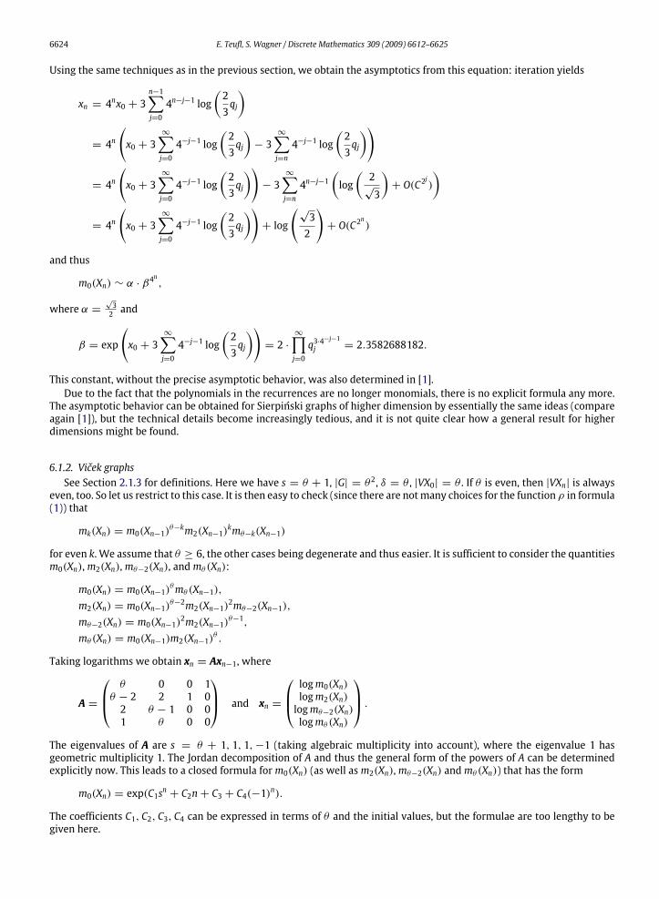
This constant, without the precise asymptotic behavior, was also determined in [1].Due to the fact that the polynomials in the recurrences are no longer monomials, there is no explicit formula any more.

The asymptotic behavior can be obtained for Sierpiński graphs of higher dimension by essentially the same ideas (compareagain [1]), but the technical details become increasingly tedious, and it is not quite clear how a general result for higherdimensions might be found.

6.1.2. Viček graphsSee Section 2.1.3 for definitions. Here we have s = θ + 1, |G| = θ2, δ = θ , |VX0| = θ . If θ is even, then |VXn| is always

even, too. So let us restrict to this case. It is then easy to check (since there are notmany choices for the function ρ in formula(1)) that

mk(Xn) = m0(Xn−1)θ−km2(Xn−1)kmθ−k(Xn−1)

for even k. We assume that θ ≥ 6, the other cases being degenerate and thus easier. It is sufficient to consider the quantitiesm0(Xn),m2(Xn),mθ−2(Xn), andmθ (Xn):

m0(Xn) = m0(Xn−1)θmθ (Xn−1),m2(Xn) = m0(Xn−1)θ−2m2(Xn−1)2mθ−2(Xn−1),mθ−2(Xn) = m0(Xn−1)2m2(Xn−1)θ−1,mθ (Xn) = m0(Xn−1)m2(Xn−1)θ .

Taking logarithms we obtain xn = Axn−1, where

A =

θ 0 0 1θ − 2 2 1 02 θ − 1 0 01 θ 0 0

and xn =

logm0(Xn)logm2(Xn)logmθ−2(Xn)logmθ (Xn)

.The eigenvalues of A are s = θ + 1, 1, 1,−1 (taking algebraic multiplicity into account), where the eigenvalue 1 hasgeometric multiplicity 1. The Jordan decomposition of A and thus the general form of the powers of A can be determinedexplicitly now. This leads to a closed formula form0(Xn) (as well asm2(Xn),mθ−2(Xn) andmθ (Xn)) that has the form

m0(Xn) = exp(C1sn + C2n+ C3 + C4(−1)n).

The coefficients C1, C2, C3, C4 can be expressed in terms of θ and the initial values, but the formulae are too lengthy to begiven here.


6.2. A special case

For simplicity we restrict to the case when VXn is always even for n > 0. As in the cases θ = 2 and θ = 3, there are alsoexamples of self-similar graphs with θ ≥ 4 (such as the Viček graphs discussed above), where the recurrences for mk(Xn)have the special form

m2k(Xn) = bk∏i

m2i(Xn−1)ak,i ,

which leads to exact formulae for the quantitiesm2k(Xn). To this end, set xk,n = logm2k(Xn) and xn = (x0,n, x1,n, . . .); then

xn = Axn−1 + c,

where A = (ak,i)k,i and c = (log bk)k. The recurrence equation above can be solved easily by means of linear algebra:

Proposition 1. For even k the quantity logmk(Xn) is given by the solution of a linear recurrence equation. Moreover, s and 1 areeigenvalues of the matrix A.

Proof. The first part is plain. Using the homogeneity of the recurrences A1 = s1 follows (1 = (1, 1, 1, . . .)). The second re-striction on the exponents of themonomials in the system (see Lemma 3) implies that Af = δ1+ f , where f = (0, 2, 4, . . .).Together with A1 = s1we obtain

A(f −

δ

s− 11)=

(f −

δ

s− 11). �

We note that in all examples the eigenvalues are±1 and s. Thus it seems plausible that this is always the case, i.e.,−1 isthe only other eigenvalue. Of course a similar result holds when the parity of |VXn| is odd or alternating.

6.3. Final remark

As demonstrated, there is no hope for closed formulae in the general case. However, the examples suggest that logm0(Xn)is always asymptotically equal to the solution of a linear recurrence. Furthermore, it is likely that such a solution containsonly powers of the form 1n, (−1)n and sn. Note that this was the case in all examples so far. Moreover, we have verified thisconjecture for the subclass where the structure of the self-similar graphs is ‘‘tree-like,’’ as for the Viček graphs.

Acknowledgment

We would like to thank two anonymous referees, whose comments and suggestions helped greatly in improving thepresentation of this paper. This material is based upon work supported by the German Research Foundation DFG undergrant number 445 SUA-113/25/0-1 and the South African National Research Foundation under grant number 65972.

References

[1] S.-C. Chang, L.-C. Chen, Dimer coverings on the Sierpiński gasketwith possible vacancies on the outmost vertices, J. Statist. Phys. 131 (4) (2008) 631–650.arXiv:0711.0573v1.

[2] J.H. Curtiss, A note on the theory of moment generating functions, Ann. Math. Statistics 13 (1942) 430–433.[3] E.J. Farrell, Matching in cacti, J. Math. Sci. (Calcutta) 8 (2) (1997) 85–96.[4] H.-K. Hwang, On convergence rates in the central limit theorems for combinatorial structures, European J. Combin. 19 (3) (1998) 329–343.[5] P.W. Kasteleyn, Graph theory and crystal physics, in: Graph Theory and Theoretical Physics, Academic Press, London, 1967, pp. 43–110.[6] J.W. Moon, The number of trees with a 1-factor, Discrete Math. 63 (1) (1987) 27–37.[7] J. Propp, Enumeration of matchings: problems and progress, in: New Perspectives in Algebraic Combinatorics, Berkeley, CA, 1996–97, in: Math. Sci.Res. Inst. Publ., vol. 38, Cambridge Univ. Press, Cambridge, 1999, pp. 255–291.

[8] E. Teufl, S. Wagner, The number of spanning trees in self-similar graphs, 2008, preprint.[9] E. Teufl, S. Wagner, Enumeration problems for classes of self-similar graphs, J. Combin. Theory Ser. A 114 (7) (2007) 1254–1277.

http://arxiv.org/0711.0573v1

Documents

Exact and asymptotic enumeration of perfect matchings in self-similar graphs