1

Exact Asymptotic Goodness-of-Fit Testing For Discrete Circular Data,

With Applications

David E. Giles

Department of Economics, University of Victoria Victoria, B.C., Canada V8W 2Y2

Revised, January 2012

Author Contact: David E. Giles, Dept. of Economics, University of Victoria, P.O. Box 1700, STN CSC, Victoria, B.C., Canada V8W 2Y2; e-mail: dgiles@uvic.ca; Phone: (250) 721-8540; FAX: (250) 721-6214

Abstract

We show that the full asymptotic null distribution for Watson’s 2NU statistic, modified for discrete

data, can be computed simply and exactly by standard methods. Previous approximate quantiles for the uniform multinomial case are found to be accurate. More extensive quantiles are presented for this distribution, as well as for the beta-binomial distribution and for the distributions associated with “Benford’s Laws”. The latter distributions are for the first one, two, or three significant digits in a sequence of “naturally occurring” numbers. A simulation experiment compares the power of the

modified 2NU test with that of Kuiper’s VN test. In addition, four empirical applications are

provided to illustrate the usefulness of the 2NU test.

Keywords: Distributions on the circle; Goodness-of-fit; Watson’s 2NU ; discrete data;

Benford’s Law Mathematics Subject Classification: 62E20; 62G10; 62G30; 62P99; 62Q05

2

1. INTRODUCTION

The construction of goodness-of-fit tests when the data are distributed on the circle (or more

generally the sphere) is an important statistical problem. An excellent discussion is provided, for

example, by Mardia and Jupp (2000). Among the tests that have been proposed for continuous data

are those based on Kuiper’s (1959) VN statistic and Watson’s (1961) 2NU statistic. These tests are of

the Kolmogorov-Smirnov type, being based on the empirical distribution function, and Castro-Kuriss

(2011) provides a concise and recent overview of such tests. Goodness-of-fit tests on the circle in the

case of discrete data are also of considerable practical importance, as we demonstrate with the

examples provided in this paper. However, this case has received far less attention in the literature.

The complication is that although Kolmogorov-Smirnov statistics are distribution-free in the

continuous case, this is generally not the case when the data are discrete (Conover, 1972). In the

latter case, modifications are needed.

We will be concerned with testing the null hypothesis, H0: “The data follow a discrete circular

distribution, F, defined by the probabilities niip 1}{ ”, against the alternative hypothesis, H1: “H0 is not

true”. Suppose that we have a sample of N observations, and let niir 1}{ denote the sample frequencies,

such that Nrn

ii

1

. For this general problem, Freedman (1981) proposes a modified version of

Watson’s 2NU statistic for use with discrete data. He provides Monte Carlo evidence that this test

out-performs Kuiper’s (1962) modified test for the discrete case, when testing the null of multinomial

uniform against the alternative of a sine-curve. Freedman’s test statistic is:

11

211

22* /)/( nj

nj jjN nSSnNU , (1)

where

j

i iij pNrS1

)/( ; j = 1, 2, …., n.

He shows that the asymptotic null distribution of the statistic in (1) is a weighted sum of (n - 1)

independent chi-squared variates, each with one degree of freedom, and with weights which are the

eigenvalues of the matrix whose (i, j)th element is

3

11

2 ),min()},max({),min()},max({)/( nk ki kjjinpjijinnp .

Freedman expresses the first four moments of the asymptotic distribution of the test statistic under H0

as functions of these eigenvalues, and uses these moments to approximate the quantiles of the

asymptotic distribution by fitting Pearson curves. He confirms the quality of this approximation by

Monte Carlo methods, just for the case where the population distribution is uniform multinomial.

In fact, however, the complete asymptotic null distribution of 2*NU can be obtained directly and

without any such approximations by using standard computational methods. Specifically, we can use

those suggested by Imhof (1961), Davies (1973, 1980) and others, to invert the characteristic

function for statistics which are weighted sums of chi-squared variates. There is no need to resort to

approximations, curve fitting or simulation methods.

In this paper we first use this information to verify and extend Freedman’s quantile calculations for

the case of uniform discrete data. Then we use Davies’ algorithm to compute the exact quantiles of

the asymptotic distributions of 2*NU when the data follow “Benford’s Laws” for the first, second and

third significant digits of a string of numbers. The use of these quantiles is then illustrated through

two examples, one of which demonstrates that correctly allowing for the discrete nature of the data

can reverse the (false) conclusion that is reached if the null hypothesis is incorrectly tested using a

test that is designed for the situation where the data are continuous.

2. ASYMPTOTIC DISTRIBUTIONS

One of the important advantages of Davies’ algorithm, in particular, is its numerical accuracy. Both

FORTRAN and C++ code for this algorithm are freely available from Davies (2011). In what follows

we use Davies’ double-precision FORTRAN code, Qf.for. The integration error bound and maximum

number of integration terms for the inversion of the characteristic function can be specified by the

user, and these were set to 10-6 and 103 respectively. The calculations were undertaken on a PC with

an Intel Pentium 3.00 GHz processor, running Windows XP Pro.

2.1 DISCRETE UNIFORM DISTRIBUTION

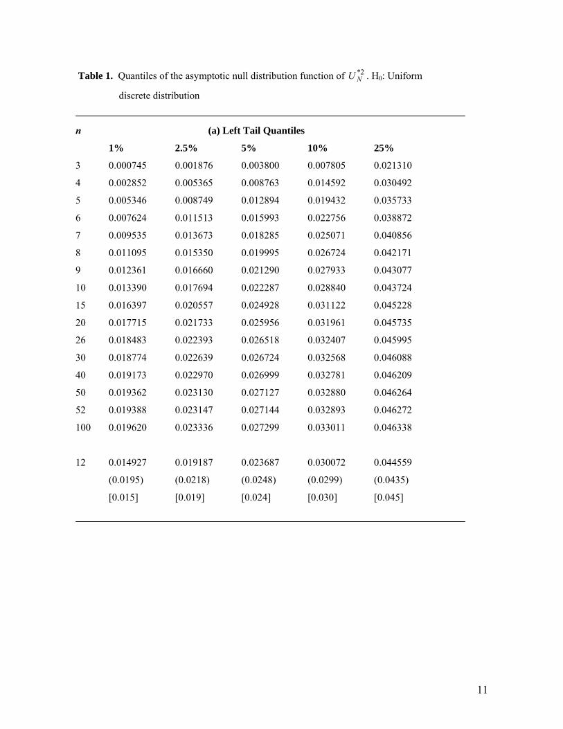
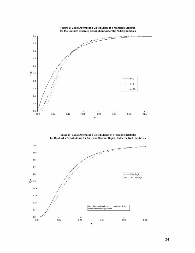
Figure 1 shows the asymptotic distribution function of 2*NU for the uniform discrete model under H0,

for selected values of n. Table 1 provides quantiles of this distribution for a wider range of n, and

4

compares these with Freeman’s approximate quantiles as appropriate. The case of n = 12 is of

interest when testing for seasonal incidence with monthly data. Freedman’s Pearson curves provide

slightly more (less) accurate upper (lower) quantiles than those obtained from Monte Carlo

simulation, when each are compared with our exact results.

2.2 BENFORD’S LAW(S)

As a second example, consider the discrete distribution usually referred to as “Benford’s Law”.

Benford (1938) re-discovered Newcomb’s (1881) observation that the first significant digit (d1) of

certain naturally occurring numbers follows the distribution given by

)]/1(1[log]Pr[ 101 iidpi ; i = 1, 2, …., 9. (2)

The “circularity” of the d1 values can be illustrated by considering the numbers 0.09 and 0.10. The

first significant digits (9 and 1) are as “distant” as possible, yet the two numbers are numerically very

close. Although we use base 10 for the logarithms in (2), and in equations (3) to (6) below, any other

consistent choice of base can be made. Various mathematical justifications for “Benford’s Law” have

been provided by several authors, including Pinkham (1961), Cohen (1976) and Hill (1995a, b, c,

1997, 1998); and Balanzario and Sánchez-Ortiz (2010) provide sufficient conditions for Benford’s

Law to hold. These conditions are very general.

The extensive bibliography by Hürlimann (2006) reflects the numerous applications of this

distribution in many disciplines. Some examples include the auditing of financial data (e.g., Drake

and Nigrini, 2000; Geyer and Williamson, 2004; Durtschi et al., 2004); examining the quality of

survey data (Judge and Schechter, 2009); the analysis hydrological records (e.g., Nigrini and Miller,

2007); image processing (e.g., Jolin, 2001; Acebo and Sbert, 2005); the α – decay half-lives of nuclei

(Ni and Ren, 2008); testing for collusion and “shilling” in eBay auctions (Giles, 2007); and testing

for the presence of psychological barriers in financial markets and auctions (e.g., De Ceuster et al.,

1998; Lu and Giles, 2010). In short, Benford’s Law is very pervasive, and frequently encountered.

For these reasons, reliable goodness-of-fit tests of this null hypothesis are of considerable interest.

Very recently Shao and Ma (2010) have linked Benford’s Law to the Fermi-Dirac, Bose-Einstein and

Boltzmann-Gibbs distributions that are of fundamental importance in statistical physics. Indeed, they

speculate: “Thus Benford’s law seems to present a general pattern for physical statistics and might be

even more fundamental and profound in nature.” (Shao and Ma, 2010, p.3109).

5

Corresponding Benford-type distributions for the higher-order significant digits are also well known.

For example, the joint distributions for the first two and first three such digits (d1, d2 and d3) are

)]10/(11[log],Pr[ 1021 jijdidp ji ; i, j = 10, 11, …., 99 (3)

and

)]10100/(11[log],,Pr[ 10321 kjikdjdidp kji ; i, j, k = 100, 101, …., 999.

(4)

Similarly, the marginal distributions for d2 and d3 are

9

1102 )]10/(11[log]Pr[

li ilidp ; i = 0, 1, …., 9 (5)

and

9

1

9

0103 )]10100/(11[log]Pr[

l mi imlidp ; i = 0, 1, …., 9. (6)

respectively.

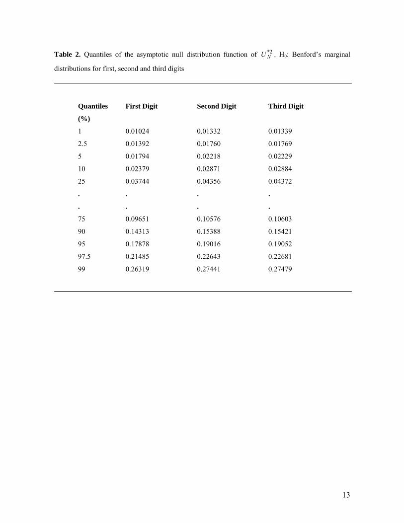
In Table 2 we present quantiles for the distribution function for 2*NU when testing against Benford’s

marginal distributions, (2), (5) and (6). Figure 2 depicts the corresponding distribution functions.

2.2 BETA-BINOMIAL DISTRIBUTION

The beta-binomial distribution is a discrete mixture distribution which can capture either under-

dispersion or over-dispersion in the data. It has been used in a diverse range of applications (e.g.,

Tong and Lord, 2007; Hunt et al., 2009; Pham et al., 2010). The probability mass function for a beta-

binomial random variable, Y, is:

),(

),(),,|.(Pr

B

ynyB

y

nnyY

; y = 0, 1, …., n ; n, α, β > 0

where B(. , .) is the usual beta function. This distribution is very versatile for modeling as its p.m.f.

can assume a wide range of shapes.

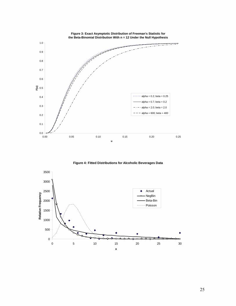
The asymptotic distribution function for 2*NU , under the null hypothesis that the data follow the beta-

binomial distribution, is illustrated in Figure 3 for n = 12, and various choices of the other

6

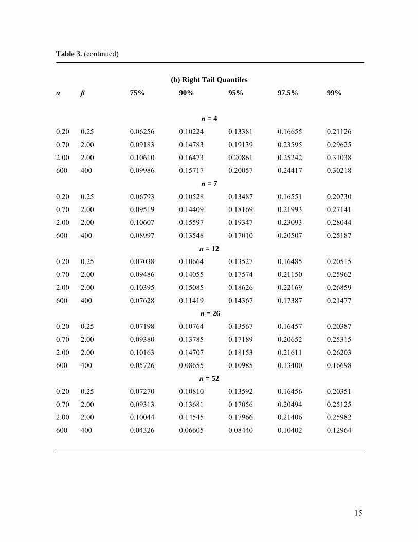
parameters. The quantiles for this distribution function are given in Table 3, where the values of n are

chosen in anticipation of applications involving daily, weekly, fortnightly, monthly, or quarterly data.

3. APPLICATIONS

3.1 CANADIAN BIRTH MONTHS

The numbers for the months of the year provide a simple example of discrete circular data, with n =

12. In one sense, December is as far from the first month of the year, January, as it can be, but in

another sense it is as close as is possible. There is a substantial demographic literature relating to

seasonality in the birth months of children. This literature suggests various reasons for non-

uniformity, and why the seasonal pattern may vary (for sociological reasons) across countries, even

those in the same hemisphere. Trovato and Odynak (1993) provide a useful discussion of seasonality

in the numbers of births in Canada.

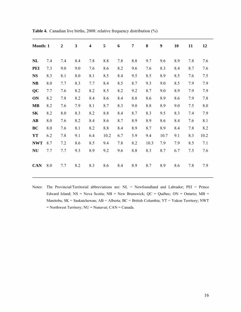
Here, we test the hypothesis of uniformity in the data for Canadian live births in 2008. These data are

from Statistics Canada (2011), and are summarized in Table 4, by Province and Territory, and for

Canada as a whole. These locations are for the mother at the time of birth.

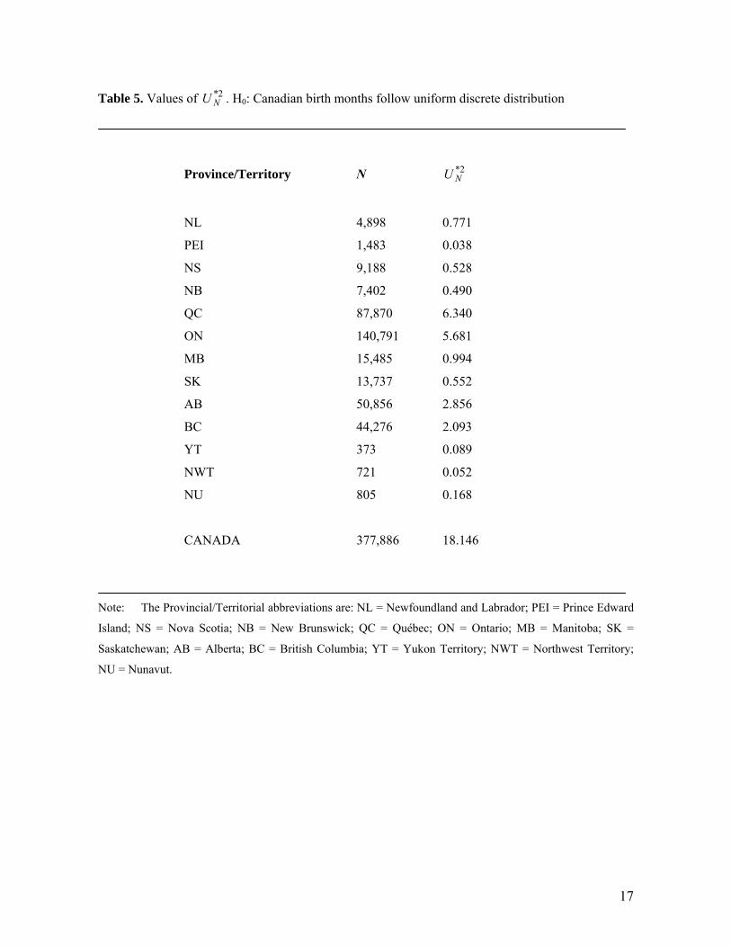
Table 5 provides the results of testing for uniformity of the distribution of births across months,

against the alternative of non-uniformity. When the 2*NU values are compared with the tabulated

critical values for n = 12 in Table 1(b), we see that the null hypothesis of uniformity is strongly

rejected for Canada as a whole, and for almost all of the provinces. It cannot be rejected for Prince

Edward Island or for the Yukon or Northwest Territories, at conventional significance levels. In the

case of Nunavut, the null hypothesis is rejected at the 10% significance level, but not at the 5% level.

Interestingly, these four exceptional cases correspond to the jurisdictions with the smallest numbers

of births in 2008. In addition, three of these four jurisdictions are located in the far North, and face

climatic and cultural situations somewhat different from the rest of Canada.

3.2 FIBONACCI SERIES AND FACTORIALS

Canessa (2003) has proposed a general statistical thermodynamic theory that explains, inter alia, why

Fibonacci sequences should obey Benford’s Law. See, also, Duncan (1969) and Washington (1981).

However, this theory has not previously been tested empirically, so here we test the hypothesis that

the distribution of the first digits of the first N numbers of the Fibonacci series, {1, 1, 2, 3, 5, 8, 13,

7

21, 34, 55, 89, 144, ……} follows Benford’s Law, for various choices of 000,20N . The

alternative hypothesis is that the distribution differs from Benford’s Law. We also test the null

hypothesis that the distribution is discrete uniform, against the alternative of non-uniformity.

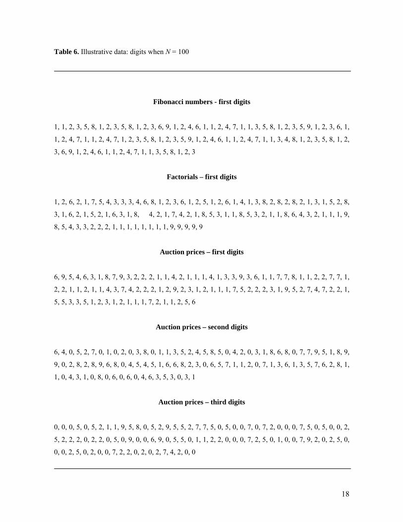
The Fibonacci first digits were generated using Knott’s (2010) Fibonacci number calculator. The

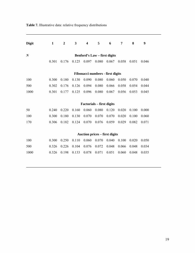
values for N = 100 appear in Table 6, and the relative frequency distributions for N = 100, 500, and

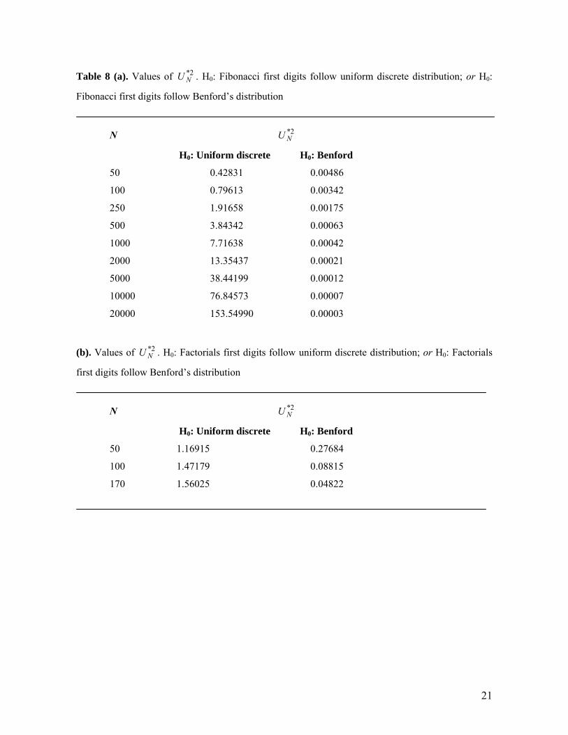
1000 are given in Table 7. For 50N , the test results in Table 8(a) indicate a clear rejection of

uniformity (using the quantiles for n = 9 in Table 1 (b)) and an equally clear non-rejection of

Benford’s first-digit Law (using the quantiles in Table 2).

Sarkar (1973) demonstrates that the first digits of factorials and binomial coefficients appear to

follow Benford’s Law. However, he does not undertake any formal goodness-of-fit testing. The first

digits of the first 100 factorials are given in Table 6, and the relative frequency distributions for N =

50, 100, and 170 appear in Table 7. The largest factorial that can be stored in computer memory is

170!. The results in Table 8(b), again using the quantiles for n = 9 from Table 1(b) and Table 2, show

a strong rejection of uniformity in each case, and failure to reject Benford’s distribution at

conventional significance levels, for N > 50.

Given the implications of the theoretical results of Duncan (1969), Washington (1981), Canesa

(2003), and Sarkar (1973), these empirical results for the Fibonacci and factorial data can be

interpreted as speaking favourably to the quality of Freedman’s test.

3.3 AUCTION PRICE DATA

Price data exhibit circularity. Consider two prices such as $99.99 and $100. Their first significant

digits are as far apart as is possible, yet the associated prices are extremely close. Giles (2007)

considered all of the 1,161 successful auctions for tickets for professional football games in the

“event tickets” category on eBay for the period 25 November to 3 December, 2004, excluding

auctions ending with the “Buy-it-Now” option, and all Dutch auctions. The winning bids should

satisfy Benford’s Law if they are “naturally occurring” numbers, as should be the case if there were

no collusion among bidders and no “shilling” by sellers in this market.

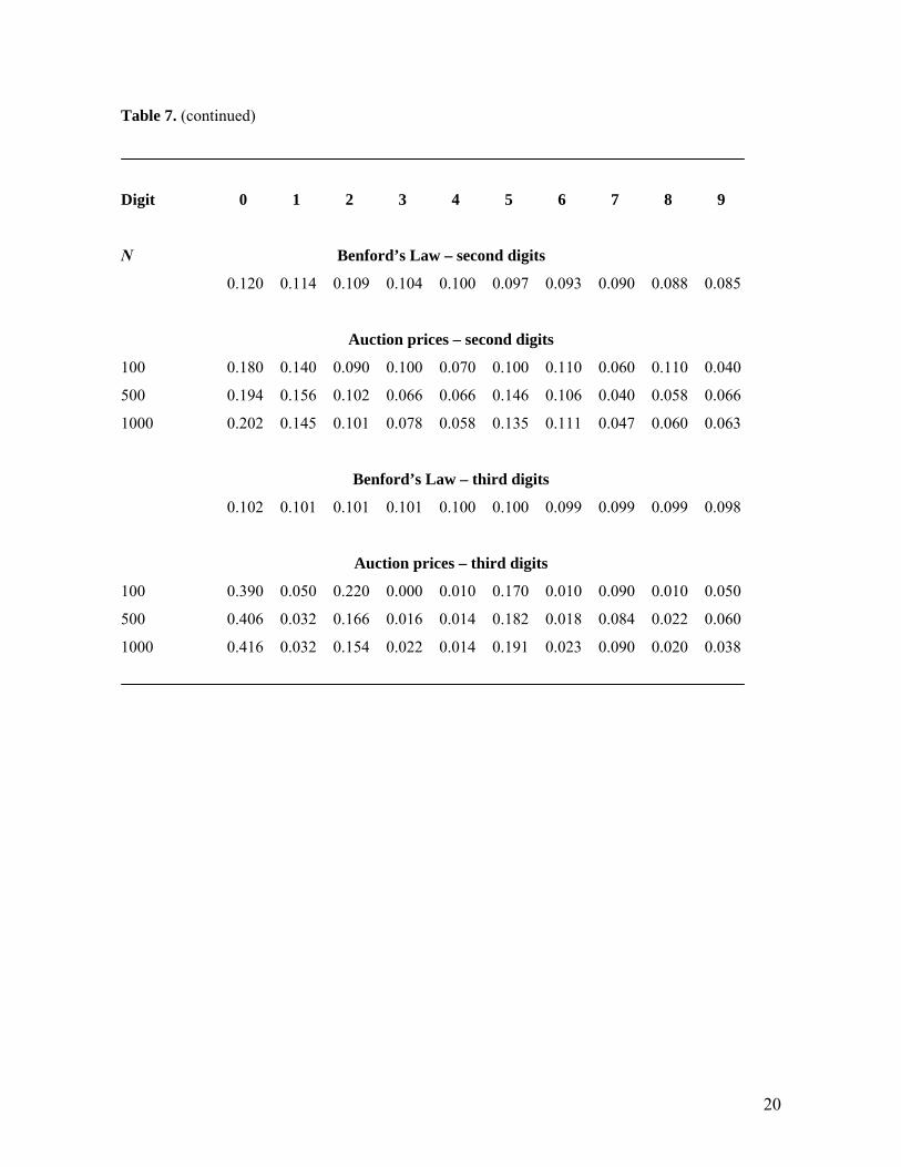
Table 6 reports the first, second, and third digits for the first 100 observations in Giles’s sample; and

Table 7 provides the relative frequency distributions for the first N = 100, 500 and 1000 sample

values. In Table 9 we see the results of testing these first, second and third digits using both the

8

uniform multinomial and Benford hypotheses. Uniformity is again strongly rejected (against non-

uniformity) for the first and third digits, and for the second digit in samples of size 250 or greater. At

the 5% significance level, Benford’s Law for the third digit is unambiguously rejected (against the

non-Benford alternative), and the first digit and second digit laws are also rejected for N > 100. In

contrast, Giles (2007) (wrongly) applied Kuiper’s (1959) VN test for continuous data to the 1,161

first-digits and marginally failed to reject Benford’s Law. (He did not consider tests for the second

and third digits, as we do here.) This comparison of our results with his illustrates the importance of

applying a test that takes account of the discrete nature of the data.

3.4 ALCOHOL CONSUMPTION DATA

Our final application fits the beta-binomial distribution to data for the number of days in a month on

which alcohol was consumed. We use a sample of 10,327 responses to the question “On how many

of the past thirty days did you drink alcoholic beverages”, in the Canadian Addiction Survey (Adlaf

et al., 2005). In this application, the data are discrete, with n = 30, but they are not circular in nature.

However, it is well known that Kuiper’s test for goodness of fit involving continuous data has good

power properties even when the data are not circular, especially if the lack of fit arises from

departures in variance.

Fitting the beta-binomial distribution to the data, using R (2008) code with the VGAM package (Yee,

2009), the maximum likelihood estimates of the parameters are 4218.0ˆ and 7021.1ˆ . The

goodness-of-fit of this distribution is compared with those of the binomial, negative binomial, and

Poisson distributions in Figure 4. We see that….. However, testing H0: beta-binomial, against the

alternative hypothesis that the distribution is not beta-binomial, we have a test statistic of 2*NU =

25.0148. For these values of n and the parameters, the 95th and 99th quantiles of the asymptotic

distribution are 0.18445 and 0.26563 respectively, so we strongly reject the hypothesis that the data

come from a beta-binomial distribution in this case.

4. POWER CONSIDERATIONS

Freedman (1981) was concerned with testing uniformity against “seasonal” fluctuations in discrete

data. He provided a limited comparison of the powers of the 2*NU test, Kuiper’s VN test, and

Edwards’ (1961) test against both sinusoidal and non-sinusoidal alternatives. The 2*NU test out-

performed the VN test, and also out-performed Edwards’ test in the non-sinusoidal case.

9

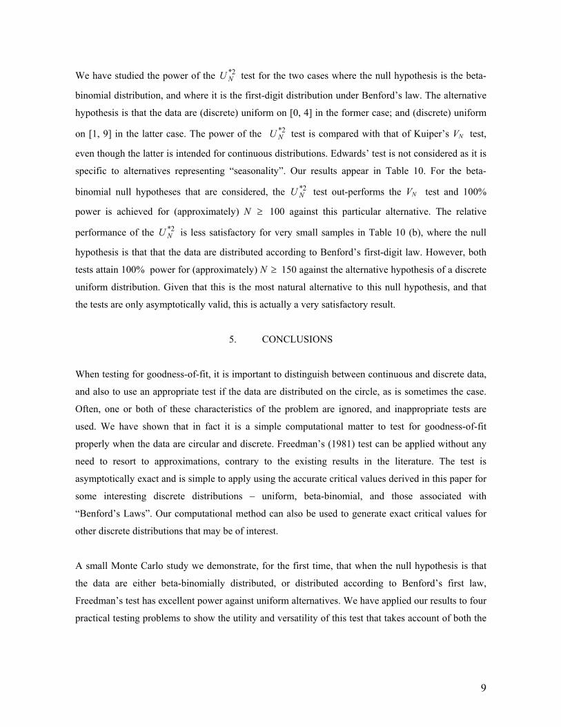
We have studied the power of the 2*NU test for the two cases where the null hypothesis is the beta-

binomial distribution, and where it is the first-digit distribution under Benford’s law. The alternative

hypothesis is that the data are (discrete) uniform on [0, 4] in the former case; and (discrete) uniform

on [1, 9] in the latter case. The power of the 2*NU test is compared with that of Kuiper’s VN test,

even though the latter is intended for continuous distributions. Edwards’ test is not considered as it is

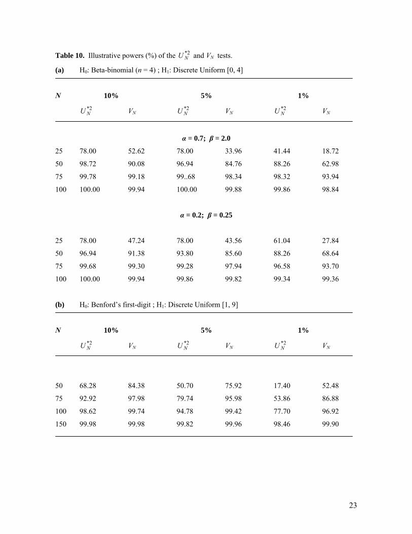
specific to alternatives representing “seasonality”. Our results appear in Table 10. For the beta-

binomial null hypotheses that are considered, the 2*NU test out-performs the VN test and 100%

power is achieved for (approximately) N 100 against this particular alternative. The relative

performance of the 2*NU is less satisfactory for very small samples in Table 10 (b), where the null

hypothesis is that that the data are distributed according to Benford’s first-digit law. However, both

tests attain 100% power for (approximately) N 150 against the alternative hypothesis of a discrete

uniform distribution. Given that this is the most natural alternative to this null hypothesis, and that

the tests are only asymptotically valid, this is actually a very satisfactory result.

5. CONCLUSIONS

When testing for goodness-of-fit, it is important to distinguish between continuous and discrete data,

and also to use an appropriate test if the data are distributed on the circle, as is sometimes the case.

Often, one or both of these characteristics of the problem are ignored, and inappropriate tests are

used. We have shown that in fact it is a simple computational matter to test for goodness-of-fit

properly when the data are circular and discrete. Freedman’s (1981) test can be applied without any

need to resort to approximations, contrary to the existing results in the literature. The test is

asymptotically exact and is simple to apply using the accurate critical values derived in this paper for

some interesting discrete distributions – uniform, beta-binomial, and those associated with

“Benford’s Laws”. Our computational method can also be used to generate exact critical values for

other discrete distributions that may be of interest.

A small Monte Carlo study we demonstrate, for the first time, that when the null hypothesis is that

the data are either beta-binomially distributed, or distributed according to Benford’s first law,

Freedman’s test has excellent power against uniform alternatives. We have applied our results to four

practical testing problems to show the utility and versatility of this test that takes account of both the

10

circularity and discrete nature of certain data. In summary, we recommend the use of Freedman’s

2*NU test for goodness-of-fit testing with discrete, possibly circular, data.

ACKNOWLEDGEMENT

I am most grateful to an anonymous referee for very helpful suggestions and comments on an earlier

version of this paper.

11

Table 1. Quantiles of the asymptotic null distribution function of 2*NU . H0: Uniform

discrete distribution

n (a) Left Tail Quantiles

1% 2.5% 5% 10% 25%

3 0.000745 0.001876 0.003800 0.007805 0.021310

4 0.002852 0.005365 0.008763 0.014592 0.030492

5 0.005346 0.008749 0.012894 0.019432 0.035733

6 0.007624 0.011513 0.015993 0.022756 0.038872

7 0.009535 0.013673 0.018285 0.025071 0.040856

8 0.011095 0.015350 0.019995 0.026724 0.042171

9 0.012361 0.016660 0.021290 0.027933 0.043077

10 0.013390 0.017694 0.022287 0.028840 0.043724

15 0.016397 0.020557 0.024928 0.031122 0.045228

20 0.017715 0.021733 0.025956 0.031961 0.045735

26 0.018483 0.022393 0.026518 0.032407 0.045995

30 0.018774 0.022639 0.026724 0.032568 0.046088

40 0.019173 0.022970 0.026999 0.032781 0.046209

50 0.019362 0.023130 0.027127 0.032880 0.046264

52 0.019388 0.023147 0.027144 0.032893 0.046272

100 0.019620 0.023336 0.027299 0.033011 0.046338

12 0.014927 0.019187 0.023687 0.030072 0.044559

(0.0195) (0.0218) (0.0248) (0.0299) (0.0435)

[0.015] [0.019] [0.024] [0.030] [0.045]

12

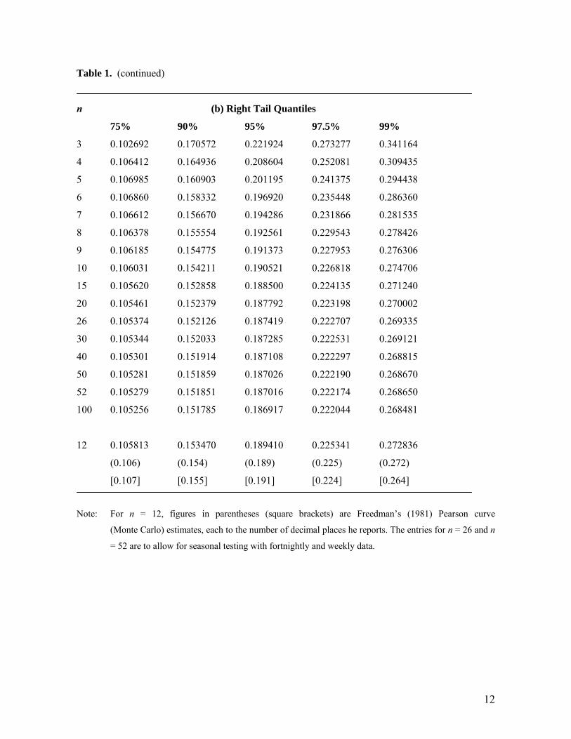
Table 1. (continued)

n (b) Right Tail Quantiles

75% 90% 95% 97.5% 99%

3 0.102692 0.170572 0.221924 0.273277 0.341164

4 0.106412 0.164936 0.208604 0.252081 0.309435

5 0.106985 0.160903 0.201195 0.241375 0.294438

6 0.106860 0.158332 0.196920 0.235448 0.286360

7 0.106612 0.156670 0.194286 0.231866 0.281535

8 0.106378 0.155554 0.192561 0.229543 0.278426

9 0.106185 0.154775 0.191373 0.227953 0.276306

10 0.106031 0.154211 0.190521 0.226818 0.274706

15 0.105620 0.152858 0.188500 0.224135 0.271240

20 0.105461 0.152379 0.187792 0.223198 0.270002

26 0.105374 0.152126 0.187419 0.222707 0.269335

30 0.105344 0.152033 0.187285 0.222531 0.269121

40 0.105301 0.151914 0.187108 0.222297 0.268815

50 0.105281 0.151859 0.187026 0.222190 0.268670

52 0.105279 0.151851 0.187016 0.222174 0.268650

100 0.105256 0.151785 0.186917 0.222044 0.268481

12 0.105813 0.153470 0.189410 0.225341 0.272836

(0.106) (0.154) (0.189) (0.225) (0.272)

[0.107] [0.155] [0.191] [0.224] [0.264]

Note: For n = 12, figures in parentheses (square brackets) are Freedman’s (1981) Pearson curve

(Monte Carlo) estimates, each to the number of decimal places he reports. The entries for n = 26 and n

= 52 are to allow for seasonal testing with fortnightly and weekly data.

13

Table 2. Quantiles of the asymptotic null distribution function of 2*NU . H0: Benford’s marginal

distributions for first, second and third digits

Quantiles First Digit Second Digit Third Digit

(%)

1 0.01024 0.01332 0.01339

2.5 0.01392 0.01760 0.01769

5 0.01794 0.02218 0.02229

10 0.02379 0.02871 0.02884

25 0.03744 0.04356 0.04372

. . . .

. . . .

75 0.09651 0.10576 0.10603

90 0.14313 0.15388 0.15421

95 0.17878 0.19016 0.19052

97.5 0.21485 0.22643 0.22681

99 0.26319 0.27441 0.27479

14

Table 3. Selected quantiles of the asymptotic null distribution function of 2*NU . H0: Beta-binomial

distribution

(a) Left Tail Quantiles

α β 1% 2.5% 5% 10% 25%

n = 4

0.20 0.25 0.00151 0.00285 0.00467 0.00782 0.01660

0.70 2.00 0.00225 0.00424 0.00695 0.01165 0.02470

2.00 2.00 0.00284 0.00534 0.00871 0.01451 0.03034

600 400 0.00257 0.00485 0.00793 0.01323 0.02784

n = 7

0.20 0.25 0.00520 0.00751 0.01036 0.01407 0.02363

0.70 2.00 0.00738 0.01071 0.01448 0.02017 0.03389

2.00 2.00 0.00944 0.01354 0.01811 0.02485 0.04055

600 400 0.00648 0.00953 0.01306 0.01844 0.03161

n = 12

0.20 0.25 0.00847 0.01103 0.01379 0.01779 0.02721

0.70 2.00 0.01171 0.01531 0.01919 0.02480 0.03783

2.00 2.00 0.00847 0.01103 0.01380 0.01779 0.02721

600 400 0.00784 0.01067 0.01379 0.01837 0.02915

n = 26

0.20 0.25 0.01117 0.01371 0.01642 0.02034 0.02957

0.70 2.00 0.01505 0.01847 0.02210 0.02731 0.03944

2.00 2.00 0.01767 0.02145 0.02543 0.03111 0.04422

600 400 0.00747 0.00958 0.01185 0.01511 0.02272

n = 52

0.20 0.25 0.01222 0.01471 0.01739 0.02127 0.03042

0.70 2.00 0.01606 0.01932 0.02279 0.02782 0.03961

2.00 2.00 0.01834 0.02191 0.02571 0.03118 0.04392

600 400 0.00622 0.00774 0.00936 0.01170 0.01721

15

Table 3. (continued)

(b) Right Tail Quantiles

α β 75% 90% 95% 97.5% 99%

n = 4

0.20 0.25 0.06256 0.10224 0.13381 0.16655 0.21126

0.70 2.00 0.09183 0.14783 0.19139 0.23595 0.29625

2.00 2.00 0.10610 0.16473 0.20861 0.25242 0.31038

600 400 0.09986 0.15717 0.20057 0.24417 0.30218

n = 7

0.20 0.25 0.06793 0.10528 0.13487 0.16551 0.20730

0.70 2.00 0.09519 0.14409 0.18169 0.21993 0.27141

2.00 2.00 0.10607 0.15597 0.19347 0.23093 0.28044

600 400 0.08997 0.13548 0.17010 0.20507 0.25187

n = 12

0.20 0.25 0.07038 0.10664 0.13527 0.16485 0.20515

0.70 2.00 0.09486 0.14055 0.17574 0.21150 0.25962

2.00 2.00 0.10395 0.15085 0.18626 0.22169 0.26859

600 400 0.07628 0.11419 0.14367 0.17387 0.21477

n = 26

0.20 0.25 0.07198 0.10764 0.13567 0.16457 0.20387

0.70 2.00 0.09380 0.13785 0.17189 0.20652 0.25315

2.00 2.00 0.10163 0.14707 0.18153 0.21611 0.26203

600 400 0.05726 0.08655 0.10985 0.13400 0.16698

n = 52

0.20 0.25 0.07270 0.10810 0.13592 0.16456 0.20351

0.70 2.00 0.09313 0.13681 0.17056 0.20494 0.25125

2.00 2.00 0.10044 0.14545 0.17966 0.21406 0.25982

600 400 0.04326 0.06605 0.08440 0.10402 0.12964

16

Table 4. Canadian live births, 2008: relative frequency distribution (%)

Month: 1 2 3 4 5 6 7 8 9 10 11 12

NL 7.4 7.4 8.4 7.8 8.8 7.8 8.8 9.7 9.6 8.9 7.8 7.6

PEI 7.3 9.0 9.0 7.6 8.6 8.2 9.6 7.6 8.3 8.4 8.7 7.6

NS 8.3 8.1 8.0 8.1 8.5 8.4 9.5 8.5 8.9 8.5 7.6 7.5

NB 8.0 7.7 8.3 7.7 8.4 8.5 8.7 9.3 9.0 8.5 7.9 7.9

QC 7.7 7.6 8.2 8.2 8.5 8.2 9.2 8.7 9.0 8.9 7.9 7.9

ON 8.2 7.8 8.2 8.4 8.6 8.4 8.8 8.6 8.9 8.6 7.9 7.8

MB 8.2 7.6 7.9 8.1 8.7 8.3 9.0 8.8 8.9 9.0 7.5 8.0

SK 8.2 8.0 8.3 8.2 8.8 8.4 8.7 8.3 9.5 8.3 7.4 7.9

AB 8.0 7.6 8.2 8.4 8.6 8.7 8.9 8.9 8.6 8.4 7.6 8.1

BC 8.0 7.6 8.1 8.2 8.8 8.4 8.9 8.7 8.9 8.4 7.8 8.2

YT 6.2 7.8 9.1 6.4 10.2 6.7 5.9 9.4 10.7 9.1 8.3 10.2

NWT 8.7 7.2 8.6 8.5 9.4 7.8 8.2 10.3 7.9 7.9 8.5 7.1

NU 7.7 7.7 9.3 8.9 9.2 9.6 8.8 8.3 8.7 6.7 7.5 7.6

CAN 8.0 7.7 8.2 8.3 8.6 8.4 8.9 8.7 8.9 8.6 7.8 7.9

Notes: The Provincial/Territorial abbreviations are: NL = Newfoundland and Labrador; PEI = Prince

Edward Island; NS = Nova Scotia; NB = New Brunswick; QC = Québec; ON = Ontario; MB =

Manitoba; SK = Saskatchewan; AB = Alberta; BC = British Columbia; YT = Yukon Territory; NWT

= Northwest Territory; NU = Nunavut; CAN = Canada.

17

Table 5. Values of 2*NU . H0: Canadian birth months follow uniform discrete distribution

Province/Territory N 2*NU

NL 4,898 0.771

PEI 1,483 0.038

NS 9,188 0.528

NB 7,402 0.490

QC 87,870 6.340

ON 140,791 5.681

MB 15,485 0.994

SK 13,737 0.552

AB 50,856 2.856

BC 44,276 2.093

YT 373 0.089

NWT 721 0.052

NU 805 0.168

CANADA 377,886 18.146

Note: The Provincial/Territorial abbreviations are: NL = Newfoundland and Labrador; PEI = Prince Edward

Island; NS = Nova Scotia; NB = New Brunswick; QC = Québec; ON = Ontario; MB = Manitoba; SK =

Saskatchewan; AB = Alberta; BC = British Columbia; YT = Yukon Territory; NWT = Northwest Territory;

NU = Nunavut.

18

Table 6. Illustrative data: digits when N = 100

Fibonacci numbers - first digits

1, 1, 2, 3, 5, 8, 1, 2, 3, 5, 8, 1, 2, 3, 6, 9, 1, 2, 4, 6, 1, 1, 2, 4, 7, 1, 1, 3, 5, 8, 1, 2, 3, 5, 9, 1, 2, 3, 6, 1,

1, 2, 4, 7, 1, 1, 2, 4, 7, 1, 2, 3, 5, 8, 1, 2, 3, 5, 9, 1, 2, 4, 6, 1, 1, 2, 4, 7, 1, 1, 3, 4, 8, 1, 2, 3, 5, 8, 1, 2,

3, 6, 9, 1, 2, 4, 6, 1, 1, 2, 4, 7, 1, 1, 3, 5, 8, 1, 2, 3

Factorials – first digits

1, 2, 6, 2, 1, 7, 5, 4, 3, 3, 3, 4, 6, 8, 1, 2, 3, 6, 1, 2, 5, 1, 2, 6, 1, 4, 1, 3, 8, 2, 8, 2, 8, 2, 1, 3, 1, 5, 2, 8,

3, 1, 6, 2, 1, 5, 2, 1, 6, 3, 1, 8, 4, 2, 1, 7, 4, 2, 1, 8, 5, 3, 1, 1, 8, 5, 3, 2, 1, 1, 8, 6, 4, 3, 2, 1, 1, 1, 9,

8, 5, 4, 3, 3, 2, 2, 2, 1, 1, 1, 1, 1, 1, 1, 1, 9, 9, 9, 9, 9

Auction prices – first digits

6, 9, 5, 4, 6, 3, 1, 8, 7, 9, 3, 2, 2, 2, 1, 1, 4, 2, 1, 1, 1, 4, 1, 3, 3, 9, 3, 6, 1, 1, 7, 7, 8, 1, 1, 2, 2, 7, 7, 1,

2, 2, 1, 1, 2, 1, 1, 4, 3, 7, 4, 2, 2, 2, 1, 2, 9, 2, 3, 1, 2, 1, 1, 1, 7, 5, 2, 2, 2, 3, 1, 9, 5, 2, 7, 4, 7, 2, 2, 1,

5, 5, 3, 3, 5, 1, 2, 3, 1, 2, 1, 1, 1, 7, 2, 1, 1, 2, 5, 6

Auction prices – second digits

6, 4, 0, 5, 2, 7, 0, 1, 0, 2, 0, 3, 8, 0, 1, 1, 3, 5, 2, 4, 5, 8, 5, 0, 4, 2, 0, 3, 1, 8, 6, 8, 0, 7, 7, 9, 5, 1, 8, 9,

9, 0, 2, 8, 2, 8, 9, 6, 8, 0, 4, 5, 4, 5, 1, 6, 6, 8, 2, 3, 0, 6, 5, 7, 1, 1, 2, 0, 7, 1, 3, 6, 1, 3, 5, 7, 6, 2, 8, 1,

1, 0, 4, 3, 1, 0, 8, 0, 6, 0, 6, 0, 4, 6, 3, 5, 3, 0, 3, 1

Auction prices – third digits

0, 0, 0, 5, 0, 5, 2, 1, 1, 9, 5, 8, 0, 5, 2, 9, 5, 5, 2, 7, 7, 5, 0, 5, 0, 0, 7, 0, 7, 2, 0, 0, 0, 7, 5, 0, 5, 0, 0, 2,

5, 2, 2, 2, 0, 2, 2, 0, 5, 0, 9, 0, 0, 6, 9, 0, 5, 5, 0, 1, 1, 2, 2, 0, 0, 0, 7, 2, 5, 0, 1, 0, 0, 7, 9, 2, 0, 2, 5, 0,

0, 0, 2, 5, 0, 2, 0, 0, 7, 2, 2, 0, 2, 0, 2, 7, 4, 2, 0, 0

19

Table 7. Illustrative data: relative frequency distributions

Digit 1 2 3 4 5 6 7 8 9

N Benford’s Law – first digits

0.301 0.176 0.125 0.097 0.080 0.067 0.058 0.051 0.046

Fibonacci numbers - first digits

100 0.300 0.180 0.130 0.090 0.080 0.060 0.050 0.070 0.040

500 0.302 0.176 0.126 0.094 0.080 0.066 0.058 0.054 0.044

1000 0.301 0.177 0.125 0.096 0.080 0.067 0.056 0.053 0.045

Factorials – first digits

50 0.240 0.220 0.160 0.060 0.080 0.120 0.020 0.100 0.000

100 0.300 0.180 0.130 0.070 0.070 0.070 0.020 0.100 0.060

170 0.306 0.182 0.124 0.070 0.076 0.059 0.029 0.082 0.071

Auction prices – first digits

100 0.300 0.250 0.110 0.060 0.070 0.040 0.100 0.020 0.050

500 0.326 0.226 0.104 0.076 0.072 0.048 0.066 0.048 0.034

1000 0.326 0.198 0.133 0.078 0.071 0.051 0.060 0.048 0.035

20

Table 7. (continued)

Digit 0 1 2 3 4 5 6 7 8 9

N Benford’s Law – second digits

0.120 0.114 0.109 0.104 0.100 0.097 0.093 0.090 0.088 0.085

Auction prices – second digits

100 0.180 0.140 0.090 0.100 0.070 0.100 0.110 0.060 0.110 0.040

500 0.194 0.156 0.102 0.066 0.066 0.146 0.106 0.040 0.058 0.066

1000 0.202 0.145 0.101 0.078 0.058 0.135 0.111 0.047 0.060 0.063

Benford’s Law – third digits

0.102 0.101 0.101 0.101 0.100 0.100 0.099 0.099 0.099 0.098

Auction prices – third digits

100 0.390 0.050 0.220 0.000 0.010 0.170 0.010 0.090 0.010 0.050

500 0.406 0.032 0.166 0.016 0.014 0.182 0.018 0.084 0.022 0.060

1000 0.416 0.032 0.154 0.022 0.014 0.191 0.023 0.090 0.020 0.038

21

Table 8 (a). Values of 2*NU . H0: Fibonacci first digits follow uniform discrete distribution; or H0:

Fibonacci first digits follow Benford’s distribution

N 2*NU

H0: Uniform discrete H0: Benford

50 0.42831 0.00486

100 0.79613 0.00342

250 1.91658 0.00175

500 3.84342 0.00063

1000 7.71638 0.00042

2000 13.35437 0.00021

5000 38.44199 0.00012

10000 76.8457 3 0.00007

20000 153.54990 0.00003

(b). Values of 2*NU . H0: Factorials first digits follow uniform discrete distribution; or H0: Factorials

first digits follow Benford’s distribution

N 2*NU

H0: Uniform discrete H0: Benford

50 1.16915 0.27684

100 1.47179 0.08815

170 1.56025 0.04822

22

Table 9. Values of 2*NU . H0: Football ticket price digits follow uniform discrete distribution; or H0:

Football ticket price digits follow Benford’s distribution

2*NU

Uniform discrete Benford

N Digit 1 Digit 2 Digit 3 Digit 1 Digit 2 Digit 3

50 0.4574 0.1242 0.3952 0.0463 0.1094 0.3883

100 1.1306 0.0476 0.2490 0.0778 0.0195 0.2407

250 3.3508 0.7566 2.7800 0.2673 0.5128 2.7390

500 5.6113 1.1440 4.8389 0.2539 0.6876 4.7680

750 8.3334 1.4935 6.9105 0.3210 0.8473 6.7987

1000 10.6368 2.1118 9.2640 0.2919 1.2482 9.1235

1161 11.7730 2.4803 11.1671 0.2258 1.4664 10.9962

23

Table 10. Illustrative powers (%) of the 2*NU and VN tests.

(a) H0: Beta-binomial (n = 4) ; H1: Discrete Uniform [0, 4]

N 10% 5% 1%

2*NU VN 2*

NU VN 2*NU VN

α = 0.7; β = 2.0

25 78.00 52.62 78.00 33.96 41.44 18.72

50 98.72 90.08 96.94 84.76 88.26 62.98

75 99.78 99.18 99..68 98.34 98.32 93.94

100 100.00 99.94 100.00 99.88 99.86 98.84

α = 0.2; β = 0.25

25 78.00 47.24 78.00 43.56 61.04 27.84

50 96.94 91.38 93.80 85.60 88.26 68.64

75 99.68 99.30 99.28 97.94 96.58 93.70

100 100.00 99.94 99.86 99.82 99.34 99.36

(b) H0: Benford’s first-digit ; H1: Discrete Uniform [1, 9]

N 10% 5% 1%

2*NU VN 2*

NU VN 2*NU VN

50 68.28 84.38 50.70 75.92 17.40 52.48

75 92.92 97.98 79.74 95.98 53.86 86.88

100 98.62 99.74 94.78 99.42 77.70 96.92

150 99.98 99.98 99.82 99.96 98.46 99.90

24

Figure 1: Exact Asymptotic Distribution of Freeman's Statistic for the Uniform Discrete Distribution Under the Null Hypothesis

0.0

0.1

0.2

0.3

0.4

0.5

0.6

0.7

0.8

0.9

1.0

0.00 0.05 0.10 0.15 0.20 0.25 0.30 0.35

u

F(u

)

n = 3

n = 6

n = 30

Figure 2: Exact Asymptotic Distributions of Freeman's Statistic for Benford's Distributions for First and Second Digits Under the Null Hypthesis

0.0

0.1

0.2

0.3

0.4

0.5

0.6

0.7

0.8

0.9

1.0

0.00 0.05 0.10 0.15 0.20 0.25

u

F(u

)

First Digit

Second Digit

Note: Distributions for second and third digits are visually indistinguishable

25

Figure 3: Exact Asymptotic Distribution of Freeman's Statistic forthe Beta-Binomial Distribution With n = 12 Under the Null Hypothesis

0.0

0.1

0.2

0.3

0.4

0.5

0.6

0.7

0.8

0.9

1.0

0.00 0.05 0.10 0.15 0.20 0.25

u

F(u

)

alpha = 0.2; beta = 0.25

alpha = 0.7; beta = 0.2

alpha = 2.0; beta = 2.0

alpha = 600; beta = 400

Figure 4: Fitted Distributions for Alcoholic Beverages Data

0

500

1000

1500

2000

2500

3000

3500

0 5 10 15 20 25 30

x

Rel

ativ

e F

req

uen

cy

Actual

NegBin

Beta-Bin

Poisson

26

REFERENCES

Acebo, E., Sbert, M., 2005. Benford’s law for natural and synthetic images. Proceedings of the First

Workshop on Computational Aesthetics in Graphics, Visualization and Imaging. Neumann,

L., Sbert, M., Gooch, B., Purgathofer, W., eds., Girona, Spain, 169-176.

Adlaf, E. M., Begin, P., Sawka, E. (eds.), 2005. Canadian Addiction Survey (CAS): A National

Survey of Canadians’ Use of Alcohol and Other Drugs: Prevalence of Use and Related

Harms. Canadian Centre on Substance Abuse, Ottawa.

Balanzario, E. P., Sánchez-Ortiz, J., 2010. Sufficient conditions for Benford’s law. Statistics and

Probability Letters, 80, 1713-1719.

Benford, F., 1938. The law of anomalous numbers. Proceedings of the American Philosophical

Society, 78, 551-572.

Canessa, E., 2003. Theory of analogous force in number sets. Physica A, 328, 44-52.

Castro-Kuriss, C., 2011. On a goodness-of-fit test for censored data from a location-scale distribution

with applications. Chilean Journal of Statistics, 2, 115-136.

Cohen, D. I. A., 1976. An explanation of the first digit phenomenon. Journal of Combinatorial

Theory, Series A, 20, 367–370.

Conover, W. J., 1972. A Kolmogorov goodness-of-fit test for discontinuous distributions. Journal of

the American Statistical Association, 67, 591-596.

Davies, R. B., 1973. Numerical inversion of a characteristic function. Biometrika, 60, 415-417.

Davies, R. B., 1980. The distribution of a linear combination of χ2 random variables, algorithm AS

155. Applied Statistics, 29, 323-333.

Davies, R. B., 2011. http://www.robertnz.net/download.html, accessed 12 March, 2011.

De Ceuster, M. K. J., Dhaene, G., Schatteman, T., 1998. On the hypothesis of psychological

barriers in stock markets and Benford’s law. Journal of Empirical Finance, 5, 263-279.

Drake, P. D., Nigrini, M. J., 2000. Computer assisted analytical procedures using Benford’s

Law. Journal of Accounting Education, 18, 127-146.

Duncan , R. L., 1969. A note on the initial digit problem. Fibonacci Quarterly, 7, 474–475.

Durtschi, C., Hillison, W., Panini, C., 2004. The effective use of Benford’s Law to assist in

detecting fraud in accounting data. Journal of Forensic Accounting, V, 17-34.

Freedman, L. S., 1981. Watson’s 2NU statistic for a discrete distribution. Biometrika, 68, 708-

711.

Geyer, C. L., Williamson, P. P., 2004. Detecting fraud in data sets using Benford’s law.

Communications in Statistics B, 33, 229-246.

27

Giles, D. E., 2007. Benford’s law and naturally occurring prices in certain eBay auctions. Applied

Economics Letters, 14, 157-161.

Hill, T. P., 1995a. Base-invariance implies Benford’s law. Proceedings of the American

Mathematical Society, 123, 887–895.

Hill, T. P., 1995b. The significant-digit phenomenon. The American Mathematical Monthly, 102,

322–327.

Hill, T. P., 1995c. A statistical derivation of the significant-digit law. Statistical Science, 10,

354–363.

Hill, T. P., 1997. Benford’s law. Encyclopedia of Mathematics Supplement, 1, 102.

Hill, T. P., 1998. The first digit phenomenon. The American Scientist, 86, 358–363.

Hunt, D. L., Cheng, C., Pounds, S., 2009. The beta-binomial distribution for estimating the

number of false rejections in microarray gene expression studies. Computational Statistics

and Data Analysis, 53, 1688-1700.

Hürlimann, W., 2006. Benford's law from 1881 to 2006. http://arxiv.org/abs/math/0607168,

accessed 11 April 2011.

Imhof, J. P., 1961. Computing the distribution of quadratic forms in normal variables. Biometrika,

48, 419-426.

Jolion, J. M., 2001. Images and Benford’s law. Journal of Mathematical Imaging and Vision, 14,

73–81.

Judge, G., Schechter, L., 2009. Detecting problems in survey data using Benford’s Law. Journal of

Human Resources, 44, 1-24.

Knott, R., 2010. http://www.mcs.surrey.ac.uk/Personal/R.Knott/Fibonacci/fibCalcX.html,

accessed 10 August 2010.

Kuiper, N. H., 1959. Alternative proof of a theorem of Birnbaum and Pyke. Annals of

Mathematical Statistics, 30, 251-252.

Kuiper, N. H., 1962. Tests concerning random points on a circle. Proceedings of the Koninklijke

Nederlandse Akademie van Wetenschappen A, 63, 38-47.

Lu, F., Giles, D. E. A., 2010. Benford’s law and psychological barriers in certain eBay auctions.

Applied Economics Letters, 17, 1005-1008.

Mardia, K. V., Jupp, P. E., 2000. Directional Statistics. Chichester: Wiley.

Newcomb, S., 1881. Note on the frequency of use of the different digits in natural numbers.

American Journal of Mathematics, 4, 39-40.

Ni, D., Ren, Z., 2008. Benford’s law and half-lives of unstable nuclei. European Physical Journal A –

Halons and Nuclei, 38, 251-255.

28

Nigrini, M. J., Miller, S. J., 2007. Benford’s Law applied to hydrology data – Results and

relevance to other geophysical data. Mathematical Geosciences, 39, 469-490.

Pham, T. V., Piersma, S. R., Warmoes, M., Jiminez, C. R., 2010. On the beta-binomial model for

analysis of spectral count data in label-free tandem mass spectrometry-based proteomics.

Bioinformatics, 26, 363-369.

Pinkham, R. S., 1961. On the distribution of first significant digits. Annals of Mathematical

Statistics, 32, 1223–1230.

R, 2008. The R Project for Statistical Computing, http://www.r-project.org, accessed 4 November

2011.

Sarkar, P. B., 1973. An observation on the significant digits of binomial coefficients and factorials.

Sankhyā B, 35, 363–364.

Shao, L., Ma, B-Q., 2010. The significant digit law in statistical physics. Physica A, 389, 3109-3116.

Statistics Canada, 2011. Cansim Database, Table 102-4502, Live births, by month, Canada,

provinces and territories, annual,

http://www5.statcan.gc.ca/cansim/a05?lang=eng&id=1024502, accessed 20 September

2011.

Tong, J., Lord, D., 2007. Investigating the application of beta-binomial models in highway

safety. Presented at the Canadian Multidisciplinary Road Safety Conference XVII, Montreal,

https://ceprofs.civil.tamu.edu/dlord/Papers/Tong_&_Lord_Beta-Binomial_Models_CMRS_

.pdf, accessed 3 October 2011.

Trovato, F., Odynak, D., 1993. The seasonality of births in Canada and the provinces, 1881-

1989: Theory and analysis. Canadian Studies in Population, 20, 1-41.

Washington, L. C., 1981. Benford's law for Fibonacci and Lucas numbers. Fibonacci Quarterly,

19, 175–177.

Watson, G. S., 1961. Goodness-of-fit tests on a circle. I. Biometrika, 48, 109-114.

Yee, T. W., 2009. VGAM: Vector generalized linear and additive models. R package version 0.7-9. http://www.stat.auckland.ac.nz/~yee/VGAM, accessed 4 November 2011.