Exact Discovery of Time Series Motifs Abdullah Mueen Eamonn Keogh Qiang Zhu Sydney Cash1,2 Brandon Westover1,3

University of California – Riverside 1Massachusetts General Hospital, 2Harvard Medical School, 3Brigham and Women's Hospital

{mueen, eamonn, qzhu}@cs.ucr.edu

ABSTRACT Time series motifs are pairs of individual time series, or subsequences of a longer time series, which are very similar to each other. As with their discrete analogues in computational biology, this similarity hints at structure which has been conserved for some reason and may therefore be of interest. Since the formalism of time series motifs in 2002, dozens of researchers have used them for diverse applications in many different domains. Because the obvious algorithm for computing motifs is quadratic in the number of items, more than a dozen approximate algorithms to discover motifs have been proposed in the literature. In this work, for the first time, we show a tractable exact algorithm to find time series motifs. As we shall show through extensive experiments, our algorithm is up to three orders of magnitude faster than brute-force search in large datasets. We further show that our algorithm is fast enough to be used as a subroutine in higher level data mining algorithms for anytime classification, near-duplicate detection and summarization, and we consider detailed case studies in domains as diverse as electroencephalograph interpretation and entomological telemetry data mining.

KEYWORDS Time Series, Motif, Exact Algorithm, Early Abandoning.

1 INTRODUCTION Time series motifs are pairs of individual time series, or subsequences of a longer time series, which are very similar to each other [19]. Figure 1 illustrates an example of a motif discovered in an industrial dataset. Since the formalism of time series motifs in 2002, dozens of researchers have used them in domains as diverse as medicine [1], entertainment [6], biology [2], telemedicine [13], telepresence [3] and severe weather prediction [22]. Because the obvious algorithm for computing motifs is quadratic in m, the number of individual time series (or the length of the single time series from which subsequences are extracted), researchers have long abandoned the hope of computing the exact solution to the motif discovery problem, and more than a dozen approximate algorithms to discover motifs have been proposed [4][7][13][23][24][27][32]. Most of these algorithms are O(m) or O(m log m) with very high constant factors. In this work, for the first time, we show a tractable exact algorithm to find time series motifs. While our exact algorithm is still worst case quadratic, we show that we can reduce the time required by three orders of magnitude. In fact, under most realistic conditions our exact algorithm is

faster than the current linear time approximate algorithms, because they have such large constant factors. As we shall show, our algorithm allows us to tackle problems which have previously been thought intractable, for example automatically constructing “dictionaries” of recurring patterns from electroencephalographs.

Figure 1: (top) The output steam flow telemetry of the Steamgen dataset has a motif of length 640 beginning at locations 589 and 8,895. (bottom) by overlaying the two motifs we can see how remarkably similar they are to each other

We further show that our algorithm is fast enough to be used as a subroutine in higher level data mining algorithms for summarization, near-duplicate detection and anytime classification [34].

1.1 Prior and Related Work A theoretical lower bound on finding the closest pair of points in d dimensional space is O(n log n) [8]. However the hidden constant term with this lower bound is exponential with the number of dimensions d. For high dimensional data (i.e. long time series) this constant overhead dominates the running time and no known algorithm is more efficient than the brute force one. As such, the brute force algorithm is the obvious choice to find time series motifs exactly. Given this, the most of the literature has focused on fast approximate algorithms for motif discovery [4][7][13][23][24][27][32], however there is one algorithm that proposes to exactly solve the time series motif problem. The FLAME algorithm of [33] is designed to find motifs in discrete strings (i.e. DNA), but the authors show that time series can be discretized and given to their algorithm. They note that their algorithm “is guaranteed to find the motif”. However, this is only true with respect to the discrete representation of the data, not with the raw time series itself. Thus the algorithm is approximate for real-valued time series. Furthermore, the algorithm is reported to take about 16 seconds to find the motif of length eleven in a financial time series of length 8,400,

0 2000 4000 6000 8000 100000

123

0 100 200 300 400 500 600 700 800

whereas our algorithm only takes 0.53 seconds (on average) to find the exact motif, with similar hardware. Approximate algorithms fare little better. For example, a recent paper on finding approximate motifs reports taking 343 seconds to find motifs in a dataset of length 32,260 [23], in contrast we can find exact motifs in similar datasets, and on similar hardware in under 100 seconds. Similarly, another very recent paper reports taking 15 minutes to find approximate motifs in a dataset of size 111,848 [4], however we can find exact motifs in similar datasets in under 4 minutes. Finally, paper [20] reports five seconds to find approximate motifs in a stock market dataset of size 12,500, whereas our exact algorithm takes less than one second. Bearing these numbers in mind, we will simply ignore other motif finding approaches for the rest of this work. To the best of our knowledge, our algorithm is completely novel. However there are related ideas in the literature. For example, [12] also exploits the information gained by the relative distances to randomly chosen reference points. However they use this information to solve the approximate similarity search problem, whereas we use it to solve the exact closest-pair problem.

2 BACKGROUND AND NOTATION Before describing our algorithm, we give definitions of the key terms used in this paper.

Definition 1: A Time Series is a sequence T=(t1,t2,…,tn) which is an ordered set of n real valued numbers.

The ordering is typically temporal; however other kinds of data such as color distributions [14], shapes [34] and spectrographs also have a well defined ordering and can fruitfully be considered “time series” for the purpose of indexing and mining. It is possible there could be variable time spacing between successive points in the series. For simplicity and without loss of generality we consider only equispaced data in this work. In general, we may have many time series to consider and thus need to define a time series database.

Definition 2: A Time Series Database (D) is an unordered set of m time series possibly of different lengths.

Again for simplicity, we assume that all the time series are of same length and D fits in the main memory (a disk-aware version of our algorithm is left for future work). Thus D is a matrix of real numbers where Di is the ith row in D as well as the ith time series Ti in the database and Di,j is the value at time j of Ti. Having a database of time series, we are now in a position to define time series motifs.

Definition 3: The Time Series Motif of a time series database D is the unordered pair of time series {Ti, Tj} in D which is the most similar among all possible pairs. More formally, ∀a,b,i,j the pair {Ti, Tj} is the motif iff dist(Ti, Tj) ≤ dist(Ta, Tb), i ≠ j and a ≠ b.

Note that our definition excludes the trivial match of a time series with itself by not allowing i ≠ j. There are some obvious possible generalizations of the above definition of time series motifs.

We can further generalize the notion of motifs by considering a motif ranking notion. More formally:

Definition 4: The kth-Time Series motif is the kth most similar pair in the database D. The pair {Ti, Tj} is the kth motif iff there exists a set S of pairs of time series of size exactly k-1 such that ∀Td ∈D {Ti,Td}∉S and {Tj,Td}∉S and ∀{Tx,Ty}∈S,{Ta,Tb}∉S dist(Tx, Ty) ≤ dist(Ti, Tj) ≤ dist(Ta, Tb).

Instead of dealing with pairs only we can also extend the notion of motifs to sets of time series that are very similar to each other.

Definition 5: The Range motif with range r is the maximal set of time series that have the property that the maximum distance between them is less than 2r. More formally S is a range motif with range r iff ∀Tx,Ty ∈S dist(Tx, Ty) ≤ 2r and ∀Td ∈D-S dist(Td, Ty) > 2r.

The range motif corresponds to dense regions or high dimensional “bumps” in time series space. We can extend these ideas to subsequences of a very long time series by treating every subsequences of length n (n << m) as an object in the time series database. Motifs in such a database are subsequences that are conserved locally in the long time series. More formally:

Definition 6: A subsequence of length n of a time series T=(t1,t2,…,tm) is a time series Ti,n = (ti,ti+1,…,ti+n-1) for 1 ≤ i ≤ m-n+1. Definition 7: The Subsequence Motif is a pair of subsequences {Ti,n, Tj,n} of a long time series T that are most similar. More formally, ∀a,b,i,j the pair {Ti,n, Tj,n} is the subsequence motif iff dist(Ti,n, Tj,n) ≤ dist(Ta,n, Tb,n), |i-j| ≥ w and |a-b| ≥ w for w > 0.

Note that we impose a constraint on the relative positions of the subsequences in the motif. This says that there should be a gap of at least w places between the subsequences. This restriction helps to prune out the trivial subsequence motifs [19]. For example (and considering discrete data for simplicity), if we were looking for motifs of length four in the string: sjdbbnvfdfpqoeutyvnABABABmbzchslfkeruyousjdq Then in this case we probably don’t want to consider the pair {ABAB ,ABAB} to be a motif, since they share 50% of their length (i.e AB is common to both). Instead, we would find the pair {sjdb, sjdq} to be a more interesting approximately repeated pattern. In this example, we can enforce this by setting the parameter w = 4. In all the definitions given above we assumed there is a meaningful way to measure the distance between two time series. There are several such ways in the literature and our method is valid for any distance measure that is a metric. We use Euclidean distance and express it as d(A,B). Recently extensive empirical comparisons have shown that the Euclidean distance is completive with or superior to more complex measures on a wide variety of domains [9]. Furthermore, its competitiveness increases as the datasets get larger (c.f. Figure 10), and it is large datasets that are of interest here.

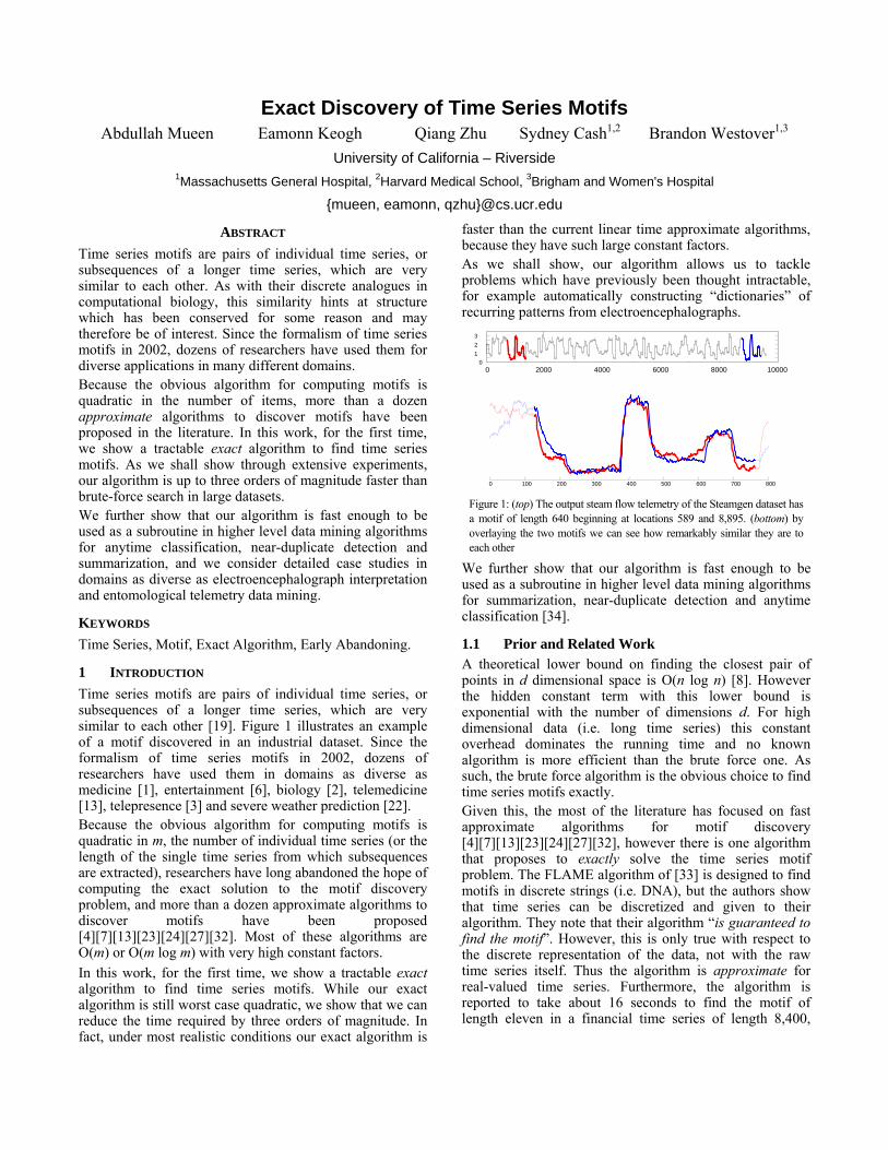
Computing the Euclidean distance between two time series of length n takes a full pass over the two time series and thus has O(n) time complexity. However when searching for the nearest neighbor for a particular time series Q, it is possible to abandon the Euclidean distance computation as soon as the cumulative sum goes beyond the current best-so-far, an idea known as early abandoning. For example assume the current best-so-far has a Euclidean distance of 12.0, and therefore a squared Euclidean distance of 144.0. If, as shown in Figure 2, the next item to be compared is further away, then at some point the sum of the squared error will exceeded the current minimum distance r=12.0 (or, equivalently r2 = 144 ). So the rest of the computation can be abandoned since this pair can’t have minimum distance. Note that we work here with the squared Euclidean distance because we can avoid having to take square roots at each of the n steps in the calculation.

Figure 2: A visual intuition of early abandoning. Once the squared sum of the accumulated gray hatch lines exceeds r2, we can be sure the full Euclidean distance exceeds r

It has long been known that early abandoning reduces the amortized cost of computing the distances to less than O(n), however, in this work we show for the first time, and explain why, early abandoning is particularly effective for motif discovery. The algorithm presented is the next section is designed for the original definition of time series motif (Definition 3 of this work). Once this problem can be solved quickly, the generalizations to the kth motif and the range motif are trivial and incur only a tiny additional overhead. Therefore, for simplicity, we will ignore these extensions in our description of the algorithm.

3 OUR ALGORITHM In Section 3.2 we have a detailed formal explanation of our exact motif discovery algorithm. However, for clarity and ease of exposition the next section contains a simple visual intuition of the underlying ideas that the algorithm exploits. We call our algorithm Mueen-Keogh (MK).

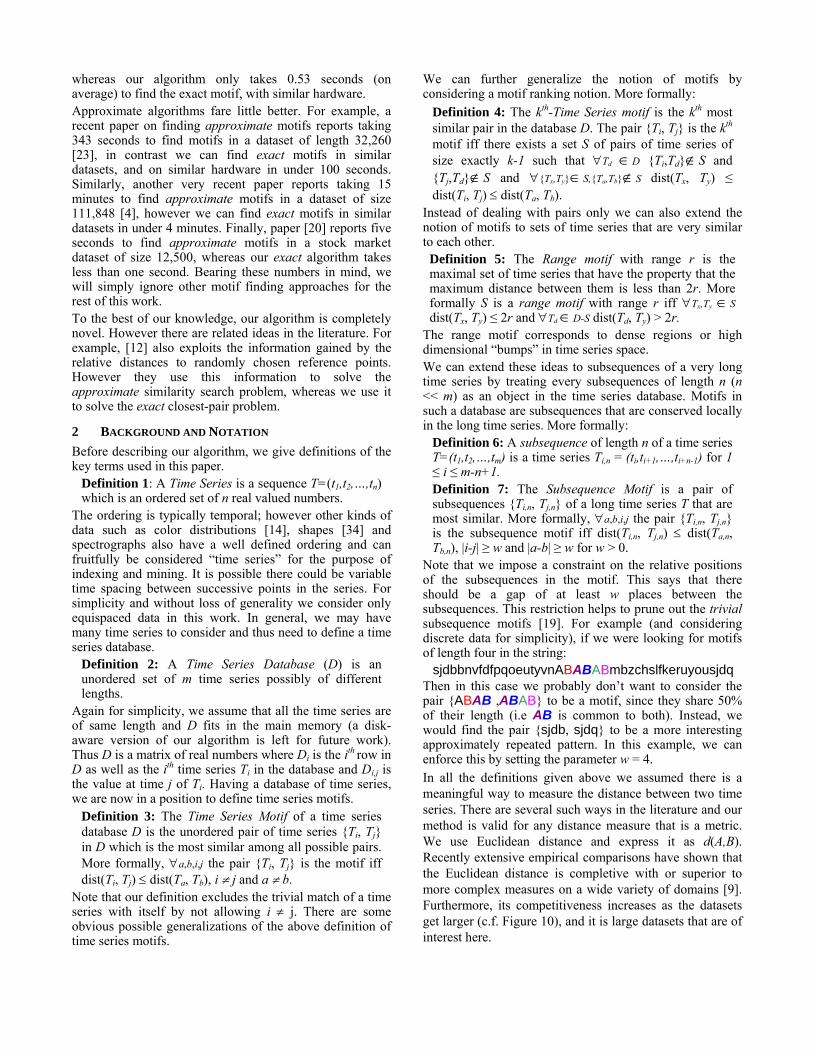
3.1 The Intuition behind our Algorithm In Figure 3.A we show a small dataset of two-dimensional time series objects. We are interested in finding the motifs, which we can see here are objects O4 and O5. Before our algorithm begins, we must assume the best-so-far distance for the motif pair to be infinity. As shown in Figure 3.B, we can choose a random object (in this case O1), as a reference point, and we can order all other objects by their distances to that point. As a side effect of this step, we can use the distance between O1 and its nearest neighbor O8, to update the best-so-far distance to be 23.0.

Note that in the act of sorting the objects we can record the distances between adjacent pairs, as shown in Figure 3.C. It is critical to recall that these distances are not (in general) the true distances between objects in the original space, rather they are lower bounds to those true distances.

Figure 3: A) A small database of two-dimensional time series objects. B) The time series objects can be arranged in a one-dimensional representation by measuring their distance to a randomly chosen point, in this case O1. C) The distances between adjacent pairs along the linear projection is a (generally weak) lower bound to the true distance between them

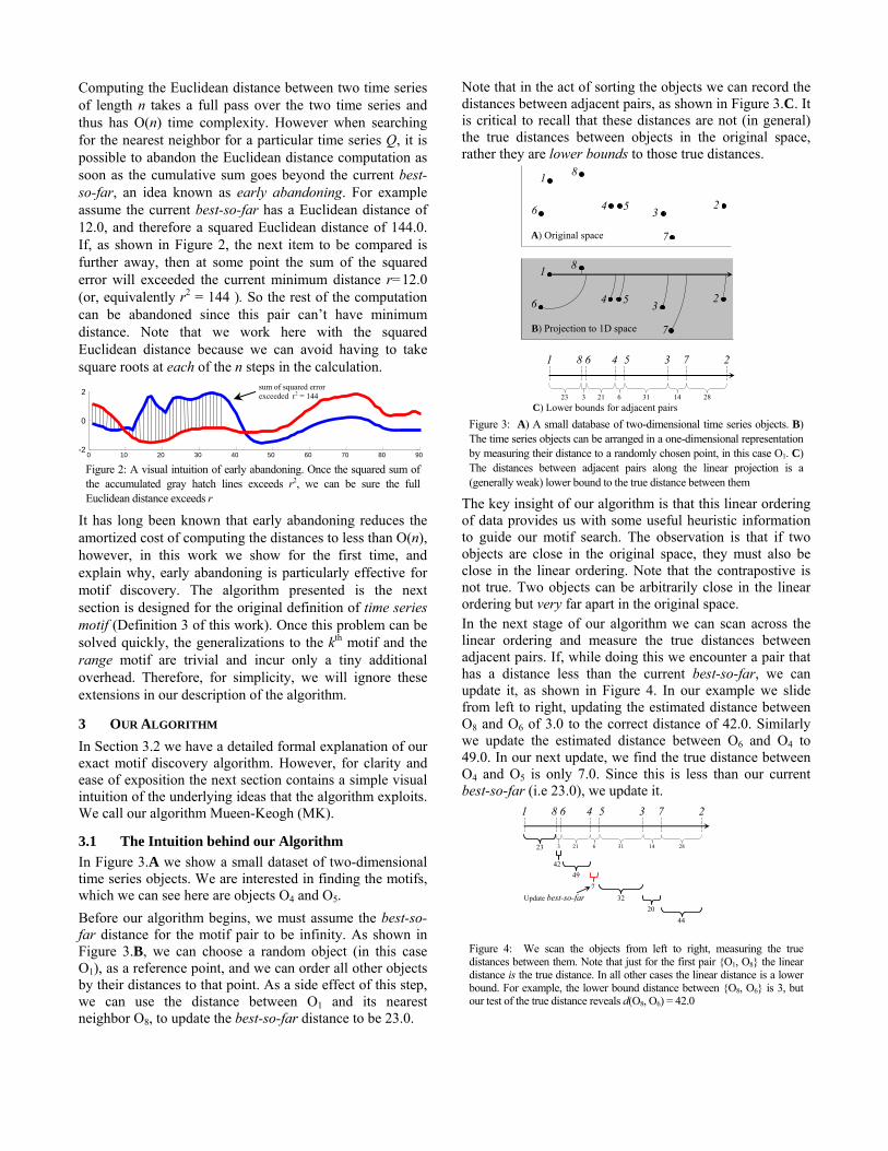
The key insight of our algorithm is that this linear ordering of data provides us with some useful heuristic information to guide our motif search. The observation is that if two objects are close in the original space, they must also be close in the linear ordering. Note that the contrapostive is not true. Two objects can be arbitrarily close in the linear ordering but very far apart in the original space. In the next stage of our algorithm we can scan across the linear ordering and measure the true distances between adjacent pairs. If, while doing this we encounter a pair that has a distance less than the current best-so-far, we can update it, as shown in Figure 4. In our example we slide from left to right, updating the estimated distance between O8 and O6 of 3.0 to the correct distance of 42.0. Similarly we update the estimated distance between O6 and O4 to 49.0. In our next update, we find the true distance between O4 and O5 is only 7.0. Since this is less than our current best-so-far (i.e 23.0), we update it.

Figure 4: We scan the objects from left to right, measuring the true distances between them. Note that just for the first pair {O1, O8} the linear distance is the true distance. In all other cases the linear distance is a lower bound. For example, the lower bound distance between {O8, O6} is 3, but our test of the true distance reveals d(O8, O6) = 42.0

1 8

6 4 5

7

3 2

1 8

6 4 5

7

3 2

1 8 6 4 5 7 3 2

23 3 21 6 31 14 28

A) Original space

B) Projection to 1D space

C) Lower bounds for adjacent pairs

1 8 6 4 5 7 3 2

23 3 21 6 31 14 28

4249

732

20 44

Update best-so-far

0 10 20 30 40 50 60 70 80 90-2

0

2 sum of squared error exceeded r2 = 144

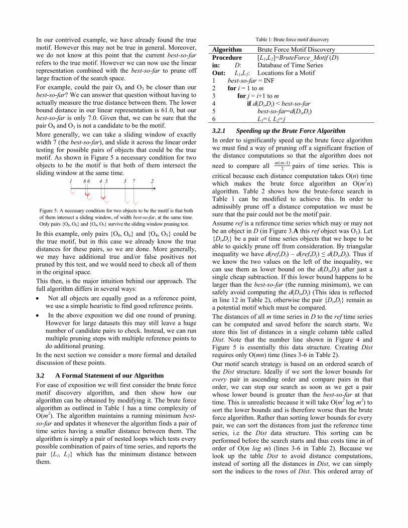
In our contrived example, we have already found the true motif. However this may not be true in general. Moreover, we do not know at this point that the current best-so-far refers to the true motif. However we can now use the linear representation combined with the best-so-far to prune off large fraction of the search space. For example, could the pair O8 and O3 be closer than our best-so-far? We can answer that question without having to actually measure the true distance between them. The lower bound distance in our linear representation is 61.0, but our best-so-far is only 7.0. Given that, we can be sure that the pair O8 and O3 is not a candidate to be the motif. More generally, we can take a sliding window of exactly width 7 (the best-so-far), and slide it across the linear order testing for possible pairs of objects that could be the true motif. As shown in Figure 5 a necessary condition for two objects to be the motif is that both of them intersect the sliding window at the same time.

Figure 5: A necessary condition for two objects to be the motif is that both of them intersect a sliding window, of width best-so-far, at the same time. Only pairs {O8, O6} and {O4, O5} survive the sliding window pruning test.

In this example, only pairs {O8, O6} and {O4, O5} could be the true motif, but in this case we already know the true distances for these pairs, so we are done. More generally, we may have additional true and/or false positives not pruned by this test, and we would need to check all of them in the original space. This then, is the major intuition behind our approach. The full algorithm differs in several ways: • Not all objects are equally good as a reference point,

we use a simple heuristic to find good reference points. • In the above exposition we did one round of pruning.

However for large datasets this may still leave a huge number of candidate pairs to check. Instead, we can run multiple pruning steps with multiple reference points to do additional pruning.

In the next section we consider a more formal and detailed discussion of these points.

3.2 A Formal Statement of our Algorithm For ease of exposition we will first consider the brute force motif discovery algorithm, and then show how our algorithm can be obtained by modifying it. The brute force algorithm as outlined in Table 1 has a time complexity of O(m2). The algorithm maintains a running minimum best-so-far and updates it whenever the algorithm finds a pair of time series having a smaller distance between them. The algorithm is simply a pair of nested loops which tests every possible combination of pairs of time series, and reports the pair {L1, L2} which has the minimum distance between them.

Table 1: Brute force motif discovery

Algorithm Brute Force Motif Discovery Procedure [L1,L2]=BruteForce_Motif (D) in: D: Database of Time Series Out: L1,L2: Locations for a Motif 1 best-so-far = INF 2 for i = 1 to m 3 for j = i+1 to m 4 if d(Di,Dj) < best-so-far 5 best-so-far=d(Di,Dj) 6 L1=i, L2=j

3.2.1 Speeding up the Brute Force Algorithm In order to significantly speed up the brute force algorithm we must find a way of pruning off a significant fraction of the distance computations so that the algorithm does not need to compare all 2

)1( −mm pairs of time series. This is critical because each distance computation takes O(n) time which makes the brute force algorithm an O(m2n) algorithm. Table 2 shows how the brute-force search in Table 1 can be modified to achieve this. In order to admissibly prune off a distance computation we must be sure that the pair could not be the motif pair. Assume ref is a reference time series which may or may not be an object in D (in Figure 3.A this ref object was O1). Let {Di,Dj} be a pair of time series objects that we hope to be able to quickly prune off from consideration. By triangular inequality we have d(ref,Di) – d(ref,Dj) ≤ d(Di,Dj). Thus if we know the two values on the left of the inequality, we can use them as lower bound on the d(Di,Dj) after just a single cheap subtraction. If this lower bound happens to be larger than the best-so-far (the running minimum), we can safely avoid computing the d(Di,Dj) (This idea is reflected in line 12 in Table 2), otherwise the pair {Di,Dj} remain as a potential motif which must be compared. The distances of all m time series in D to the ref time series can be computed and saved before the search starts. We store this list of distances in a single column table called Dist. Note that the number line shown in Figure 4 and Figure 5 is essentially this data structure. Creating Dist requires only O(mn) time (lines 3-6 in Table 2). Our motif search strategy is based on an ordered search of the Dist structure. Ideally if we sort the lower bounds for every pair in ascending order and compare pairs in that order, we can stop our search as soon as we get a pair whose lower bound is greater than the best-so-far at that time. This is unrealistic because it will take O(m2 log m2) to sort the lower bounds and is therefore worse than the brute force algorithm. Rather than sorting lower bounds for every pair, we can sort the distances from just the reference time series, i.e the Dist data structure. This sorting can be performed before the search starts and thus costs time in of order of O(m log m) (lines 3-6 in Table 2). Because we look up the table Dist to avoid distance computations, instead of sorting all the distances in Dist, we can simply sort the indices to the rows of Dist. This ordered array of

1 8 6 4 5 7 3 2

indices is named as I in Table 2 at line 7. Formally, I is the sorted order of the time series in D where d(ref,DI(i)) ≤ d(ref,DI(j)) iff i≤ j. Before considering how we will search this linear ordering, we must introduce the variable offset. The offset is simply an integer between 1 and m-1. If we point to the jth item in the ordered list I, and to the jth + offset item, then we have a candidate pair of time series which we may test. As we will see below, if we consider systematic values of j and offset, we can guarantee that we have considered or eliminated all possible pairs of candidates. To see how the ordering in list I will guide the search and help the search finish early, we must first consider the following two lemmas.

Table 2: Speeded up brute force motif discovery

Algorithm Speeded up Brute Force Motif Discovery Procedure [L1,L2]=SpeededUp_Motif(D) 1 best-so-far = INF 2 ref=a randomly chosen time series Dr from D 3 for j=1 to m 4 Distj=d(ref,Dj) 5 if Dist,j < best-so-far 6 best-so-far = Disti , L1=r, L2=j 7 find an ordering I of the indices to the time series in

D such that DistI(j)≤DistI(j+1) 8 offset=0, abandon=false 9 while abandon=false 10 offset=offset+1, abandon=true 11 for j=1 to m-offset 12 if DistI(j) - DistI(j+offset)<best-so-far 13 abandon=false 14 if d(DI(j),DI(j+offset))<best-so-far 15 Best-so-far=d(DI(j),DI(j+offset)) 16 L1=I(j),L2=I(j+offset)

Lemma 1: If DI(j+offset)-DI(j) > best-so-far for all 1≤ j ≤m-offset and offset > 0 then DI(j+w)-DI(j) > best-so-far for all 1≤ j ≤m-w and w>offset.

In other words; for a positive integer offset and for j=1,2…,m-offset if {DI(j),DI(j+offset)} fail to have their lower bounds less than the best-so-far then for all positive integers w>offset and for all j=1,2,…,m-w, {DI(j),DI(j+w)} will also fail to have their lower bounds less than the best-so-far. This is true from the definition of I,

d(ref,DI(j)) ≤ d(ref,DI(j+offset)) ≤ d(ref,DI(j+w)). This can be rewritten as

d(ref,DI(j+offset)) - d(ref,DI(j)) ≤ d(ref,DI(j+w)) - d(ref,DI(j)). So if the left part is larger than best-so-far the right part will obviously be larger.

Lemma 2: If offset=1,2,…,m-1 and j=1,2,…,m-offset then {DI(j),DI(j+offset)} generates all the 2

)1( −mm pairs.

If we search the database D for all possible offsets by which two time series can be apart in D we must encounter all the possible pairs. Since I has no repetition, it is obvious that {DI(j),DI(j+offset)} will generate all the pairs with no

repetition. Hence this lemma states the exactness of our search strategy. With the help of these two lemmas we can build the search strategy. The algorithm starts with an initial offset of 1 and searches pairs that are offset apart in the I ordering. After searching all pairs of offset apart, it increase the offset and search again (for the next round). The algorithm continues till it reaches an offset for which there is no pair having lower bound larger than the best-so-far and staying offset apart in the I ordering, at that point we can admissibly abandon the search with the exact motif pair. Lines 8 to 13 of Table 2 detail this search strategy. Clearly this strategy has the worst case complexity O(m2), which is equal to the brute force algorithm. However this only occurs in the cases where the motif has distance larger than any lower bound computed using a random reference. In thousands of experiments with real world datasets this never happened.

3.2.2 Generalization to multiple reference points The speed up that we gained in the previous section can be extended to consider multiple reference time series and we can use them to have tighter lower bounds. Using multiple reference time series raises some issues in our previous version. We show the final version of our algorithm in Table 3.

Table 3: MK motif Discovery

Algorithm MK Motif Discovery Procedure [L1,L2]=MK_Motif (D,R) 1 best-so-far = INF 2 for i=1 to R 3 refi=a randomly chosen time series Dr from D 4 for j=1 to m 5 Disti,j=d(refi,Dj) 6 if Disti,j < best-so-far 7 best-so-far= Disti,j , L1=r, L2=j 8 Si=standard_deviation(Disti) 9 find an ordering Z of the indices to the reference time

series in ref such that SZ(i)≥SZ(i+1) 10 find an ordering I of the indices to the time series in

D such that DistZ(1),I(j)≤DistZ(1),I(j+1) 11 offset=0, abandon=false 12 while abandon=false 13 offset=offset+1, abandon=true 14 for j=1 to m 15 reject=false 16 for i=1 to R 17 lower_bound=|DistZ(i),I(j) - DistZ(i),I(j+offset)| 18 if lower_bound > best-so-far 19 reject=true, break 20 else if i = 1 21 abandon=false 22 if reject=false 23 if d(DI(j),DI(j+offset))<best-so-far 24 best-so-far=d(DI(j),DI(j+offset)) 25 L1=I(j),L2=I(j+offset)

To get the tighter lower bounds we use multiple reference time series, which we randomly chosen from D as before. The number of reference points is a parameter to our algorithm represented by R. Obviously this introduction does not change the outcome of the algorithm. As we will later see (cf. Figure 8), once this number is greater than 5 or 6, its exact value does not even change the running time. As a consequence of using multiple references, Dist becomes a two dimensional table that stores distances between any reference time series to any time series in D. The way multiple references help tightening the lower bounds is very simple. We simply use the maximum of the lower bounds. This is correct because if one lower bound is larger than best-so-far the maximum would also be larger and there is no way the pair would become a motif. Since the lower bounds are not stored anywhere, the algorithm needs to compute all the R lower bounds for every single pair (lines 16-17 in Table 3). Rather than computing the maximum which would take O(R) time, we compare each bound with the current best-so-far and reject (line 19 in Table 3) computing the true distance as soon as one bound is higher than the best-so-far. Thus amortized cost of the combined lower bound is smaller than O(R). Although multiple reference time series tighten the lower bounds, we cannot use all of them in ordering the search strategy. This is because we need to follow exactly one ordering (Lemma 2) to guide our search (lines 20-21 in Table 3). To choose a reference time series for ordering the time series in D, we select the one (Z(1) in line 10) with the largest standard deviation in the distances from itself to others in D (lines 9-10 in Table 3). The intuition behind this is simply that the larger the standard deviation is, the larger the lower bounds will be.

4 SCALABILITY EXPERIMENTS We begin by stating our experimental philosophy. We have designed all experiments such that they are not only reproducible, but easily reproducible. To this end, we have built a webpage (http://www.cs.ucr.edu/~mueen/MK) which contains all datasets and code used in this work, together with spreadsheets which contain the raw numbers displayed in all the figures. In addition, the webpage contains many additional experiments which we could not fit into this work; however, we note that this paper is completely self-contained. We performed the scalability experiments on both synthetic and real data. All the experiments are performed on a computer with an AMD 2.1GHz Turion X2 Ultra ZM-80 processor and 3.0GB of DDR2 memory. The algorithm is coded in C and compiled with gcc. As we noted in Section 1.1, our exact algorithm is faster than all current approximate algorithms (that choose to report time), so we only compare to two variants of exact search.

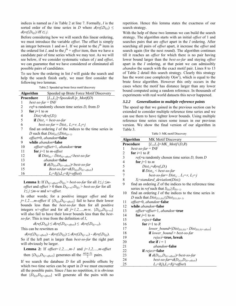
4.1 Performance Comparison As a starting point we use random walk time series to test our algorithm. Random walk data is a difficult case for our algorithm, since we should not expect a very close motif pair to exist in the data. We produced 10 sets of random walks of different sizes containing from 10,000 to 100,000 time series, all of length 1024. We ran our algorithm 10 times on each of these datasets and took the average of the execution times. Figure 6 shows a comparison of the brute force algorithm with our MK algorithm in terms of the execution time.

Figure 6: A comparison of three algorithms in the time taken to find the motif pair in increasingly large random walk databases. For the brute force algorithm, values for dataset sizes beyond 30,000 are extrapolated

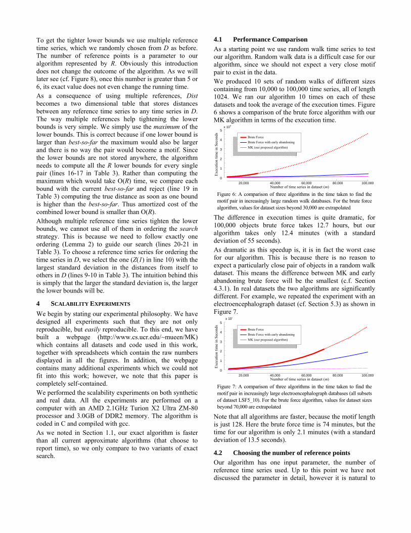
The difference in execution times is quite dramatic, for 100,000 objects brute force takes 12.7 hours, but our algorithm takes only 12.4 minutes (with a standard deviation of 55 seconds). As dramatic as this speedup is, it is in fact the worst case for our algorithm. This is because there is no reason to expect a particularly close pair of objects in a random walk dataset. This means the difference between MK and early abandoning brute force will be the smallest (c.f. Section 4.3.1). In real datasets the two algorithms are significantly different. For example, we repeated the experiment with an electroencephalograph dataset (cf. Section 5.3) as shown in Figure 7.

Figure 7: A comparison of three algorithms in the time taken to find the motif pair in increasingly large electroencephalograph databases (all subsets of dataset LSF5_10). For the brute force algorithm, values for dataset sizes beyond 70,000 are extrapolated

Note that all algorithms are faster, because the motif length is just 128. Here the brute force time is 74 minutes, but the time for our algorithm is only 2.1 minutes (with a standard deviation of 13.5 seconds).

4.2 Choosing the number of reference points Our algorithm has one input parameter, the number of reference time series used. Up to this point we have not discussed the parameter in detail, however it is natural to

20,000 40,000 60,000 80,000 100,0000

1

2

3

4

5 x 104

Number of time series in dataset (m)

Exec

utio

n tim

e in

Sec

onds

Brute ForceBrute Force with early abandoning MK (our proposed algorithm)

20,000 40,000 60,000 80,000 100,0000

1

2

3

4

5 x 103

Number of time series in dataset (m)

Exec

utio

n tim

e in

Sec

onds

Brute ForceBrute Force with early abandoning MK (our proposed algorithm)

ask how critical its setting is. A simple thought experiment tells us that a too small or too large value should produce a slower algorithm. In the former case, if few reference time series are used, most candidate pairs are not pruned, and must be examined by brute force. In the latter case, we may have only O(m) pairs of candidates left to check, but the time to create a one-dimensional representation from a reference time series is O(m), so we may not break even and we may have been better off to just brute force the remaining time series. This reasoning tells us that a plot of execution time vs. number of reference time series should be a U-shaped curve, and we should target a parameter that gives us the bottom of the curve. In Figure 8 we illustrate this observation with an experiment in varying the number of reference points and measuring the execution time. Note that the leftmost value, corresponding to zero reference point is equivalent to the special case of brute force search.

Figure 8: A plot of execution time vs. the number of reference points. Note that once the number of reference points is beyond say five, its exact value makes little difference. Note the log scale of the time axis

This plot suggests that the input parameter is not critical. Any value from five to sixty gives two orders of magnitude speedup. Moreover, this is true if we change the length of the time series, the size of the database (i.e m) or the data type. For this reason, we fixed the number of reference points to be eight in all the experiments in this paper.

4.3 Discussion and Interpretation of Results In the following sections we interpret and explain the results of the scalability results in more detail.

4.3.1 Why is Early-Abandoning so Effective? While the results in the previous section bode well for the MK algorithm, a perhaps unexpected result is that just using early-abandoning can make brute force search significantly faster. While it has been known for some time that early-abandoning can speed up nearest neighbor search; most work suggests that the speedup is a small constant, in the range of two to three [18]. However, at least for the random walk experiment shown in Figure 6 it appears early-abandoning can produce at least a ten-fold speed up. It is informative to consider why this is so. The power of early-abandoning comes from the (relative) value of the best-so-far variable during search. If it has a small value early on in a search, then most items can be abandoned very early. However, we typically have no control over how fast the best-so-far decreases; we simply hope that a relatively similar object will be encountered early in the search.

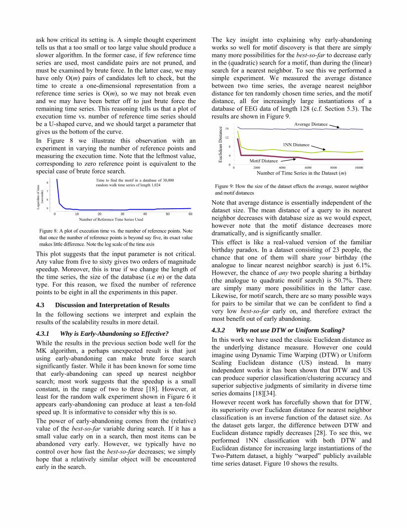
The key insight into explaining why early-abandoning works so well for motif discovery is that there are simply many more possibilities for the best-so-far to decrease early in the (quadratic) search for a motif, than during the (linear) search for a nearest neighbor. To see this we performed a simple experiment. We measured the average distance between two time series, the average nearest neighbor distance for ten randomly chosen time series, and the motif distance, all for increasingly large instantiations of a database of EEG data of length 128 (c.f. Section 5.3). The results are shown in Figure 9.

Figure 9: How the size of the dataset effects the average, nearest neighbor and motif distances

Note that average distance is essentially independent of the dataset size. The mean distance of a query to its nearest neighbor decreases with database size as we would expect, however note that the motif distance decreases more dramatically, and is significantly smaller. This effect is like a real-valued version of the familiar birthday paradox. In a dataset consisting of 23 people, the chance that one of them will share your birthday (the analogue to linear nearest neighbor search) is just 6.1%. However, the chance of any two people sharing a birthday (the analogue to quadratic motif search) is 50.7%. There are simply many more possibilities in the latter case. Likewise, for motif search, there are so many possible ways for pairs to be similar that we can be confident to find a very low best-so-far early on, and therefore extract the most benefit out of early abandoning.

4.3.2 Why not use DTW or Uniform Scaling? In this work we have used the classic Euclidean distance as the underlying distance measure. However one could imagine using Dynamic Time Warping (DTW) or Uniform Scaling Euclidean distance (US) instead. In many independent works it has been shown that DTW and US can produce superior classification/clustering accuracy and superior subjective judgments of similarity in diverse time series domains [18][34]. However recent work has forcefully shown that for DTW, its superiority over Euclidean distance for nearest neighbor classification is an inverse function of the dataset size. As the dataset gets larger, the difference between DTW and Euclidean distance rapidly decreases [28]. To see this, we performed 1NN classification with both DTW and Euclidean distance for increasing large instantiations of the Two-Pattern dataset, a highly “warped” publicly available time series dataset. Figure 10 shows the results.

Number of Time Series in the Dataset (m)

0

4

8

12

16

0 2000 4000 6000 8000 10000

Motif Distance

1NN Distance

Average Distance

Eucl

idea

n D

ista

nce

0 10 20 30 40 50 60

5 6 7 8

Loga

rithm

of t

ime

(sec

onds

)

Number of Reference Time Series Used

Time to find the motif in a database of 30,000random walk time series of length 1,024

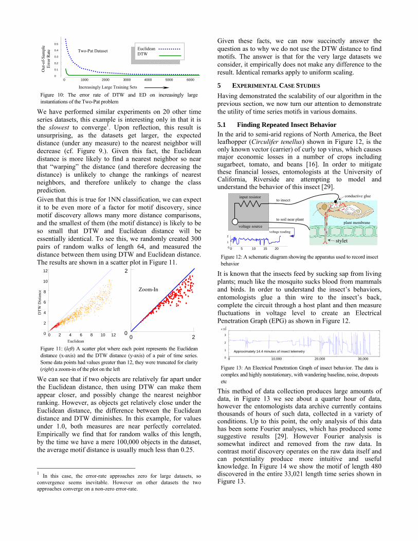
Figure 10: The error rate of DTW and ED on increasingly large instantiations of the Two-Pat problem

We have performed similar experiments on 20 other time series datasets, this example is interesting only in that it is the slowest to converge1. Upon reflection, this result is unsurprising, as the datasets get larger, the expected distance (under any measure) to the nearest neighbor will decrease (cf. Figure 9.). Given this fact, the Euclidean distance is more likely to find a nearest neighbor so near that “warping” the distance (and therefore decreasing the distance) is unlikely to change the rankings of nearest neighbors, and therefore unlikely to change the class prediction. Given that this is true for 1NN classification, we can expect it to be even more of a factor for motif discovery, since motif discovery allows many more distance comparisons, and the smallest of them (the motif distance) is likely to be so small that DTW and Euclidean distance will be essentially identical. To see this, we randomly created 300 pairs of random walks of length 64, and measured the distance between them using DTW and Euclidean distance. The results are shown in a scatter plot in Figure 11.

Figure 11: (left) A scatter plot where each point represents the Euclidean distance (x-axis) and the DTW distance (y-axis) of a pair of time series. Some data points had values greater than 12, they were truncated for clarity (right) a zoom-in of the plot on the left

We can see that if two objects are relatively far apart under the Euclidean distance, then using DTW can make them appear closer, and possibly change the nearest neighbor ranking. However, as objects get relatively close under the Euclidean distance, the difference between the Euclidean distance and DTW diminishes. In this example, for values under 1.0, both measures are near perfectly correlated. Empirically we find that for random walks of this length, by the time we have a mere 100,000 objects in the dataset, the average motif distance is usually much less than 0.25.

1 In this case, the error-rate approaches zero for large datasets, so convergence seems inevitable. However on other datasets the two approaches converge on a non-zero error-rate.

Given these facts, we can now succinctly answer the question as to why we do not use the DTW distance to find motifs. The answer is that for the very large datasets we consider, it empirically does not make any difference to the result. Identical remarks apply to uniform scaling.

5 EXPERIMENTAL CASE STUDIES Having demonstrated the scalability of our algorithm in the previous section, we now turn our attention to demonstrate the utility of time series motifs in various domains.

5.1 Finding Repeated Insect Behavior In the arid to semi-arid regions of North America, the Beet leafhopper (Circulifer tenellus) shown in Figure 12, is the only known vector (carrier) of curly top virus, which causes major economic losses in a number of crops including sugarbeet, tomato, and beans [16]. In order to mitigate these financial losses, entomologists at the University of California, Riverside are attempting to model and understand the behavior of this insect [29].

Figure 12: A schematic diagram showing the apparatus used to record insect behavior

It is known that the insects feed by sucking sap from living plants; much like the mosquito sucks blood from mammals and birds. In order to understand the insect’s behaviors, entomologists glue a thin wire to the insect’s back, complete the circuit through a host plant and then measure fluctuations in voltage level to create an Electrical Penetration Graph (EPG) as shown in Figure 12.

Figure 13: An Electrical Penetration Graph of insect behavior. The data is complex and highly nonstationary, with wandering baseline, noise, dropouts etc

This method of data collection produces large amounts of data, in Figure 13 we see about a quarter hour of data, however the entomologists data archive currently contains thousands of hours of such data, collected in a variety of conditions. Up to this point, the only analysis of this data has been some Fourier analyses, which has produced some suggestive results [29]. However Fourier analysis is somewhat indirect and removed from the raw data. In contrast motif discovery operates on the raw data itself and can potentiality produce more intuitive and useful knowledge. In Figure 14 we show the motif of length 480 discovered in the entire 33,021 length time series shown in Figure 13.

plant membrane

stylet

voltage source

input resistor

0 5 10 15 200

1

2

to soil near plant

to insectconductive glue

voltage reading

0 10,000 20,000 30,0000

1

2

3

x 104

Approximately 14.4 minutes of insect telemetry

0 2 4 6 8 10 12 0 2 4 6 8 10 12

0 20

2

Euclidean

DTW

Dis

tanc

e Zoom-In

2000 3000 4000 5000 60000 0.1 0.2 0.3 0.4 0.5

0 1000 Two-Pat Dataset Euclidean

DTW Increasingly Large Training Sets

Out

-of-

Sam

ple

Er

ror R

ate

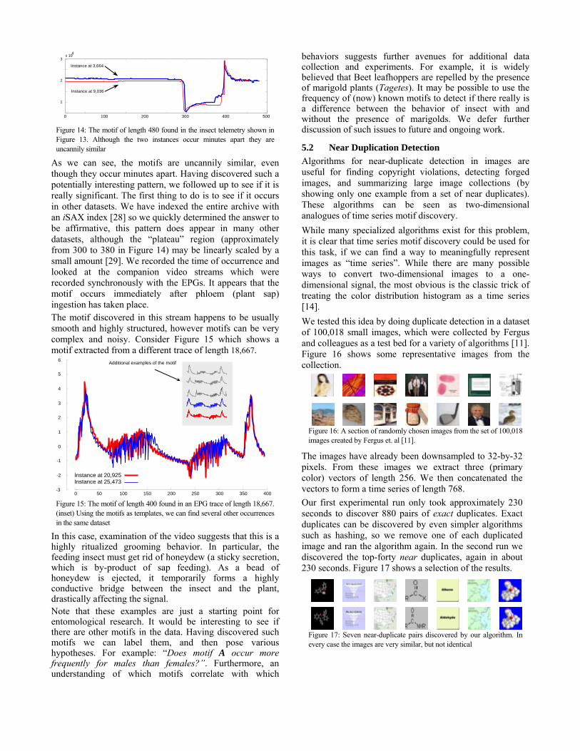
Figure 14: The motif of length 480 found in the insect telemetry shown in Figure 13. Although the two instances occur minutes apart they are uncannily similar

As we can see, the motifs are uncannily similar, even though they occur minutes apart. Having discovered such a potentially interesting pattern, we followed up to see if it is really significant. The first thing to do is to see if it occurs in other datasets. We have indexed the entire archive with an iSAX index [28] so we quickly determined the answer to be affirmative, this pattern does appear in many other datasets, although the “plateau” region (approximately from 300 to 380 in Figure 14) may be linearly scaled by a small amount [29]. We recorded the time of occurrence and looked at the companion video streams which were recorded synchronously with the EPGs. It appears that the motif occurs immediately after phloem (plant sap) ingestion has taken place. The motif discovered in this stream happens to be usually smooth and highly structured, however motifs can be very complex and noisy. Consider Figure 15 which shows a motif extracted from a different trace of length 18,667.

Figure 15: The motif of length 400 found in an EPG trace of length 18,667. (inset) Using the motifs as templates, we can find several other occurrences in the same dataset

In this case, examination of the video suggests that this is a highly ritualized grooming behavior. In particular, the feeding insect must get rid of honeydew (a sticky secretion, which is by-product of sap feeding). As a bead of honeydew is ejected, it temporarily forms a highly conductive bridge between the insect and the plant, drastically affecting the signal. Note that these examples are just a starting point for entomological research. It would be interesting to see if there are other motifs in the data. Having discovered such motifs we can label them, and then pose various hypotheses. For example: “Does motif A occur more frequently for males than females?”. Furthermore, an understanding of which motifs correlate with which

behaviors suggests further avenues for additional data collection and experiments. For example, it is widely believed that Beet leafhoppers are repelled by the presence of marigold plants (Tagetes). It may be possible to use the frequency of (now) known motifs to detect if there really is a difference between the behavior of insect with and without the presence of marigolds. We defer further discussion of such issues to future and ongoing work.

5.2 Near Duplication Detection Algorithms for near-duplicate detection in images are useful for finding copyright violations, detecting forged images, and summarizing large image collections (by showing only one example from a set of near duplicates). These algorithms can be seen as two-dimensional analogues of time series motif discovery. While many specialized algorithms exist for this problem, it is clear that time series motif discovery could be used for this task, if we can find a way to meaningfully represent images as “time series”. While there are many possible ways to convert two-dimensional images to a one-dimensional signal, the most obvious is the classic trick of treating the color distribution histogram as a time series [14]. We tested this idea by doing duplicate detection in a dataset of 100,018 small images, which were collected by Fergus and colleagues as a test bed for a variety of algorithms [11]. Figure 16 shows some representative images from the collection.

Figure 16: A section of randomly chosen images from the set of 100,018 images created by Fergus et. al [11].

The images have already been downsampled to 32-by-32 pixels. From these images we extract three (primary color) vectors of length 256. We then concatenated the vectors to form a time series of length 768. Our first experimental run only took approximately 230 seconds to discover 880 pairs of exact duplicates. Exact duplicates can be discovered by even simpler algorithms such as hashing, so we remove one of each duplicated image and ran the algorithm again. In the second run we discovered the top-forty near duplicates, again in about 230 seconds. Figure 17 shows a selection of the results.

Figure 17: Seven near-duplicate pairs discovered by our algorithm. In every case the images are very similar, but not identical

0 100 200 300 400 500

1

2

3 x 10 4

Instance at 9,036

Instance at 3,664

Additional examples of the motif

0 50 100 150 200 250 300 350 400 -3

-2

-1

0

1

2

3

4

5

6

Instance at 20,925 Instance at 25,473

Using brute-force search to find these, it takes 37 minutes using the early abandoning optimization and approximately 6 hours without the early abandoning.

5.3 Automatically Constructing EEG Dictionaries In this example of the utility of time series motifs we discuss an ongoing joint project between the authors and Physicians at Massachusetts General Hospital (MGH) in automatically constructing “dictionaries” of recurring patterns from electroencephalographs. The electroencephalogram (EEG) measures voltage differences across the scalp and reflects the activity of large populations of neurons underlying the recording electrode [26]. Figure 18 shows a sample snippet of EEG data. Medical situations in which EEG plays an important role include, diagnosing and treating epilepsy; planning brain surgery for patients with intractable epilepsy, monitoring brain activity during cardiac surgery and in certain comatose patients; and distinguishing epileptic seizures from other medical conditions (e.g. “psudoseizures”). The interpretation of EEG data involves inferring information about the brain (e.g. presence and location of a brain lesion) or brain state (e.g. awake, sleeping, having a seizure) from various temporal and spatial patterns, or graphoelements (which we see as motifs), within the EEG data stream. Over the roughly 100 years since its invention in the early 1900s, electroencephalographers have identified a small collection of clinically meaningful motifs, including entities named “spike-and-wave complexes”, “wicket spikes”, “K-complexes”, “sleep spindles” and “alpha waves”, among many other examples. However, the full “dictionary” of motifs that comprise the EEG contains potentially many yet-undiscovered motifs. In addition, the current, known motifs have been determined based on subjective analysis rather than a principled search. A more complete knowledge of the full complement of EEG motifs may well lead to new insights into the structure of cortical activity in both normal circumstances and in pathological situations including epilepsy, dementia and coma.

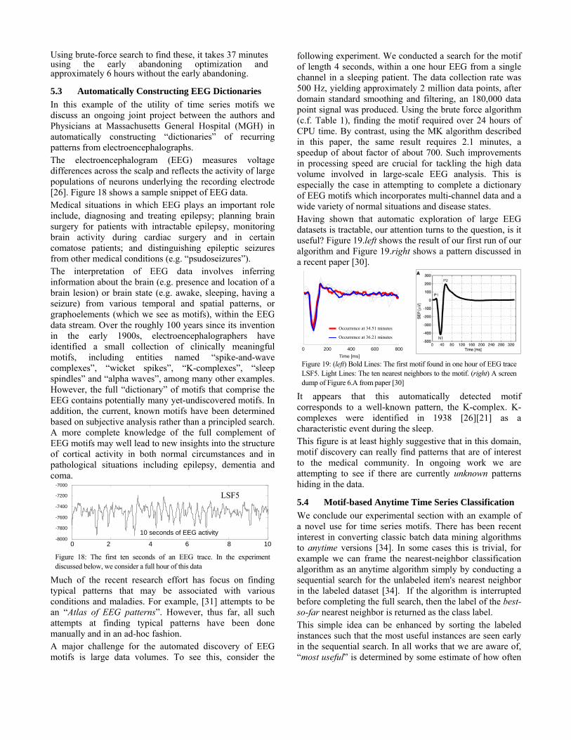
Figure 18: The first ten seconds of an EEG trace. In the experiment discussed below, we consider a full hour of this data

Much of the recent research effort has focus on finding typical patterns that may be associated with various conditions and maladies. For example, [31] attempts to be an “Atlas of EEG patterns”. However, thus far, all such attempts at finding typical patterns have been done manually and in an ad-hoc fashion. A major challenge for the automated discovery of EEG motifs is large data volumes. To see this, consider the

following experiment. We conducted a search for the motif of length 4 seconds, within a one hour EEG from a single channel in a sleeping patient. The data collection rate was 500 Hz, yielding approximately 2 million data points, after domain standard smoothing and filtering, an 180,000 data point signal was produced. Using the brute force algorithm (c.f. Table 1), finding the motif required over 24 hours of CPU time. By contrast, using the MK algorithm described in this paper, the same result requires 2.1 minutes, a speedup of about factor of about 700. Such improvements in processing speed are crucial for tackling the high data volume involved in large-scale EEG analysis. This is especially the case in attempting to complete a dictionary of EEG motifs which incorporates multi-channel data and a wide variety of normal situations and disease states. Having shown that automatic exploration of large EEG datasets is tractable, our attention turns to the question, is it useful? Figure 19.left shows the result of our first run of our algorithm and Figure 19.right shows a pattern discussed in a recent paper [30].

Figure 19: (left) Bold Lines: The first motif found in one hour of EEG trace LSF5. Light Lines: The ten nearest neighbors to the motif. (right) A screen dump of Figure 6.A from paper [30]

It appears that this automatically detected motif corresponds to a well-known pattern, the K-complex. K-complexes were identified in 1938 [26][21] as a characteristic event during the sleep. This figure is at least highly suggestive that in this domain, motif discovery can really find patterns that are of interest to the medical community. In ongoing work we are attempting to see if there are currently unknown patterns hiding in the data.

5.4 Motif-based Anytime Time Series Classification We conclude our experimental section with an example of a novel use for time series motifs. There has been recent interest in converting classic batch data mining algorithms to anytime versions [34]. In some cases this is trivial, for example we can frame the nearest-neighbor classification algorithm as an anytime algorithm simply by conducting a sequential search for the unlabeled item's nearest neighbor in the labeled dataset [34]. If the algorithm is interrupted before completing the full search, then the label of the best-so-far nearest neighbor is returned as the class label. This simple idea can be enhanced by sorting the labeled instances such that the most useful instances are seen early in the sequential search. In all works that we are aware of, “most useful” is determined by some estimate of how often

0 2 4 6 8 10-8000 -7800 -7600 -7400 -7200 -7000

LSF5

10 seconds of EEG activity

0 200 400 600 800

Occurrence at 34.51 minutes

Occurrence at 36.21 minutes

Time [ms]

each instance is used to correctly predict, as opposed to incorrectly predict, unknown instances [34][35]. The astute reader will immediately see a potential weakness here. Suppose we happen to have two nearly identical instances with the same class label in the training dataset. Furthermore, suppose they both happen to be useful instances (in the sense discussed above). In this case, both of the instances will be pushed to the head of the sequential search array. However, this is clearly redundant; we should push either one, but not both top, of the sequential search array. Time series motifs potentially allow a fix for this problem. We can discover the 1st motif, and then move one of the pair to the head of the sequential search array. Then we can rerun motif discovery on the remaining m-1 time series (excluding the recently moved object) again move one of the motif pair to the front, and begin motif discovery on m-2 objects etc. This strategy should ensure high diversity of the first few training examples encountered by the anytime classification algorithm. We tested this simple idea against random ordering, and a well known ordering algorithm called Drop3 [35]. We considered two publicly available datasets, CBF and Face4.

Figure 20: The out-of-sample accuracy of three different ordering techniques on two benchmark time series datasets. The y-axis shows the accuracy of 1NN if the algorithm is interrupted after seeing x objects

The results are quite surprising. The motif ordering algorithm is significantly better than Drop3, even though it does not consider any information about how useful any individual instance is; it is merely enhancing the diversity seen by the classifier in the early part of the nearest neighbor search. While we found similar results for other datasets, the difference between motif ordering and Drop3 diminishes as we consider larger training sets. Nevertheless, these results do suggest a promising avenue for future research. Could a hybrid of motif ordering and Drop3 outperform either one?

6 CONCLUSIONS AND FUTURE WORK We have introduced the first exact motif search algorithm which is significantly faster than brute force search. We have further demonstrated the utility of motif discovery in a variety of data mining tasks. Our work focuses on a single, simple definition of motif. However we argue that this definition can be used to efficiently find any other reasonable definition. For example, if “motif” is defined as a set of K time series, all within r of each other, or a set of K time series each within r of at least one other, then it is clear that both definitions

require at least one pair of time series to be within r of each other. We can therefore use MK to find such a pair, then use similarity search to fill in the missing K-2 time series that complete the set under the respective definitions. The question of the best definition for motifs is probably not as important as it might seem. The entomological, electroencephalograph and image motifs shown in Section 5 are essentially unchanged under different definitions of motif. There has been some work on alterative definitions of motifs, for example [20] promises to “significantly improve the quality of motifs”. However, our floccinaucinihilipilification of this work is based on the fact that the evaluation metric used was tautological, there is simply zero evidence to show the alternative definition is useful in any sense. Future and ongoing work includes extensive case studies in several domains, including space telemetry, entomology and electroencephalography, and creating a disk aware version of our algorithm to allow the exploration of truly massive datasets. ACKNOWLEDGEMENTS: We would like to thank all the donors of datasets. We particularly thank Candice Stafford and Gregory P. Walker of the Entomological Dept. of UCR for their assistance with interpreting the Beet leafhopper data. This work was funded by NSF awards 0803410 and NSF 0808770. We are also grateful to them.

REFERENCE [1] H. Abe and T. Yamaguchi, Implementing an integrated

time-series data mining environment – a case study of medical kdd on chronic hepatitis, presented at the 1st International Conference on Complex Medical Engineering (CME2005), 2005.

[2] I. Androulakis, J. Wu, J. Vitolo and C. Roth, Selecting maximally informative genes to enable temporal expression profiling analysis, Proc. of Foundations of Systems Biology in Engineering, 2005.

[3] D. Arita, H. Yoshimatsu, and R. Taniguchi, Frequent motion pattern extraction for motion recognition in real-time human proxy, Proc. of JSAI Workshop on Conversational Informatics, pp. 25–30, 2005.

[4] P. Beaudoin, M. van de Panne, P. Poulin and S. Coros, Motion-Motif Graphs, Symposium on Computer Animation 2008.

[5] C. Böhm and F. Krebs, High Performance Data Mining Using the Nearest Neighbor Join, Proc. of 2nd IEEE International Conference on Data Mining (ICDM), pp. 43-50, 2002.

[6] B. Celly and V. Zordan, Animated people textures, Proc. of 17th International Conference on Computer Animation and Social Agents (CASA), 2004.

[7] B. Chiu, E. Keogh, and S. Lonardi, Probabilistic discovery of time series motifs, Proc. of the 9th International Conference on Knowledge Discovery and Data mining (KDD’03), pp. 493–498, 2003.

0 5 10 15 20 25 30 010 20 30 40 50 60 70 80 90

0 5 10 15 20 25

Random ordering Drop3 Motif ordering

CBF Dataset Face Four Dataset

Number of instances seen before interruption

Acc

urac

y

[8] T. H. Cormen, C. E. Leiserson, R. L. Rivest, C. Stein, Introduction to Algorithms, 2nd Edition, The MIT Press, McGraw Hill Book Company, 2001.

[9] H. Ding, G. Trajcevski, P. Scheuermann, X. Wang and E. Keogh, Querying and Mining of Time Series Data: Experimental Comparison of Representations and Distance Measures, VLDB 2008.

[10] F. Duchêne, C. Garbay and V. Rialle, Learning recurrent behaviors from heterogeneous multivariate time-series, Artificial Intelligence in Medicine 39(1): 25-47 (2007).

[11] A. Torralba, R. Fergus and W. T. Freeman, 80 million Tiny Images: a Large Database for Non-Parametric Object and Scene Recognition, IEEE PAMI, 30(11):1958-1970, November, 2008.

[12] E. C. Gonzalez, K. Figueroa and G. Navarro, Effective Proximity Retrieval by Ordering Permutations, IEEE Transactions on Pattern Analysis and Machine Intelligence, 30(9):1647 – 1658, 2008.

[13] T. Guyet, C. Garbay and M. Dojat, Knowledge construction from time series data using a collaborative exploration system, Journal of Biomedical Informatics 40(6): 672-687 (2007).

[14] J. Hafner, H. Sawhney, et al, Efficient color histogram indexing for quadratic form distance functions, IEEE Trans. on Pattern Analysis and Machine Intelligence, 17(7):729--736, 1995.

[15] R. Hamid, S. Maddi, A. Johnson, A. Bobick, I. Essa, and C. Isbell. Unsupervised activity discovery and characterization from event-streams, Proc. of the 21st Conference on Uncertainty in Artificial Intelligence (UAI05), 2005.

[16] S. Kaffka, B. Wintermantel, M. Burk, and G. Peterson, Protecting high-yielding sugarbeet varieties from loss to curly top, 2000. http://sugarbeet.ucdavis.edu/Notes/Nov00a.htm

[17] E. J. Keogh, Efficiently Finding Arbitrarily Scaled Patterns in Massive Time Series Databases, Proc. of the 7th European Conference on Principles and Practice of Knowledge Discovery in Databases (PKDD), pp. 253-265, 2003.

[18] E. J. Keogh, L. Wei, X. Xi, S-H Lee and M. Vlachos: LB_Keogh Supports Exact Indexing of Shapes under Rotation Invariance with Arbitrary Representations and Distance Measures, pp. 882-893, VLDB 2006.

[19] J. Lin, E. Keogh, S. Lonardi, and P. Patel, Finding motifs in time series, Proc. of 2nd Workshop on Temporal Data Mining (KDD’02), 2002.

[20] Z. Liu, J. X. Yu, X. Lin, H. Lu and W. Wang, Locating Motifs in Time-Series Data, Pacific-Asia Conference on Knowledge Discovery and Data Mining. 2005.

[21] A.L. Loomis, E. Harvey, and G. Hobart, Disturbance patterns in sleep, J. Neurophysiol., 2 (1938) 413-430.

[22] A. McGovern, D. Rosendahl, A. Kruger, M. Beaton, R. Brown, and K. Droegemeier, Understanding the formation of tornadoes through data mining, 5th Conference on Artificial Intelligence and its

Applications to Environmental Sciences at the American Meteorological Society, 2007.

[23] J. Meng, J.Yuan, M. Hans and Y. Wu, Mining Motifs from Human Motion, Proc. of EUROGRAPHICS, 2008.

[24] D. Minnen, C.L. Isbell, I. Essa, and T. Starner, Discovering Multivariate Motifs using Subsequence Density Estimation and Greedy Mixture Learning, 22nd Conf. on Artificial Intelligence (AAAI’07), 2007.

[25] K. Murakami, S. Doki, S. Okuma, and Y. Yano, A study of extraction method of motion patterns observed frequently from time-series posture data, Proc. of IEEE International Conference on Systems, Man and Cybernetics (SMC), pp. 3610–3615, 2005.

[26] E. Niedermeyer. and F. Lopes da Silva. (Editors). Electroencephalography: Basic Principles, Clinical Applications and Related Fields. Baltimore, MD: Williams and Wilkins, 1999.

[27] S. Rombo and G. Terracina, Discovering representative models in large time series databases, Proc. of the 6th International Conference on Flexible Query Answering Systems, pp. 84–97, 2004.

[28] J. Shieh and E. Keogh, iSAX: Indexing and Mining Terabyte Sized Time Series, SIGKDD. pp 623-631 2008.

[29] C. Stafford and G. Walker, Characterization and correlation of DC electrical penetration graph waveforms with feeding behavior of beet leafhopper, under submission, 2008.

[30] B. J. Stefanovic, W. Schwindt, M. Hoehn and A. C. Silva, Functional uncoupling of hemodynamic from neuronal response by inhibition of neuronal nitric oxide synthase, Journal of Cerebral Blood Flow & Metabolism, 27: 741–754, 2007.

[31] J. M. Stern and J. Engel Jr., Atlas of EEG patterns, Lippincott, Williams & Wilkins, 2004.

[32] Y. Tanaka, K. Iwamoto, and K. Uehara, Discovery of time-series motif from multi-dimensional data based on MDL principle, Machine Learning, 58(2-3):269–300, 2005.

[33] S. Tata, Declarative Querying For Biological Sequences, Ph.d Thesis, The University of Michigan, 2007. (Advisor Jignesh M. Patel).

[34] K. Ueno, X. Xi, E. Keogh and D. Lee, Anytime Classification Using the Nearest Neighbor Algorithm with Applications to Stream Mining, Proc. of IEEE International Conference on Data Mining (ICDM), 2006.

[35] D. R. Wilson and T. R. Martinez, Reduction techniques for instance-based learning algorithms, Machine Learning, Vol 38, pages 257-286, Kluwer Acadamic Publishers, 2000.