Exchange rate volatility and exchange rate …Munich Personal RePEc Archive Exchange rate volatility and exchange rate uncertainty in Nigeria: a ﬁnancial econometric analysis (1970-

Munich Personal RePEc Archive

Exchange rate volatility and exchangerate uncertainty in Nigeria: a financialeconometric analysis (1970- 2012)

nnamdi, Kelechi and ifionu, Ebele

university of port harcourt, Nigeria

2013

Online at https://mpra.ub.uni-muenchen.de/48316/

MPRA Paper No. 48316, posted 15 Jul 2013 15:43 UTC

0

Exchange rate volatility and exchange rate uncertainty in Nigeria: a financial

econometric analysis

(1970- 2012)

By

Kelechi C. Nnamdi

University of Port Harcourt, Nigeria Email: [email protected]

&

Ebele P. Ifionu, Ph.D.

University of Port Harcourt, Nigeria Email: [email protected]

ABSTRACT

This research paper examines exchange rate volatility over time (1970-2012) using the

Generalized Autoregressive Conditional Heteroscedasticity (AR GARCH) model of the

Maximum Likelihood techniques. Our AR GARCH result showed that lagged (last year)

exchange rate is significantly responsible for the dynamics of Naira/ Dollar exchange rate in

Nigeria. Most glaring is that our ARCH and GARCH parameters indicate that exchange rate

volatility shocks are rather persistent in Nigeria. We also find that exchange rate uncertainty has

a direct relationship with current exchange rate in Nigeria. Further, the Granger causality test

conducted shows that the direction of causality is more powerful and significant from exchange

rate uncertainty to actual exchange rate in Nigeria. Thus the paper suggests a proper

management of exchange rate, to forestall costly distortions in the Nigerian economy.

Keywords: GARCH Models, Financial Econometrics, Foreign Exchange rate, Monetary Policy

JEL Classification: C22, C58, F31, E52

Paper to be Presented at the Eighteenth Annual Conference of the African Econometric Society, Accra, Ghana

mailto:[email protected]

http://www.africametrics.org/conferences/2013/index.html

1

1. Introduction

Foreign exchange rate as generally defined in economic literature is the rate at which one

country’s currency can be traded for another country’s currency. While exchange rate volatility,

implies the liability of a country’s currency relative to another country’s currency to fluctuate

over time. Exchange rate volatility could depend on two basic policies, that is the fixed exchange

rate policy and the flexible exchange rate policy. By fixed exchange rate policy (regime), we

mean a situation, when the exchange rate is set and government is committed to buying and

selling its currency at a fixed rate, while flexible exchange rate policy defines a situation when

the exchange rate is set by market forces (demand and supply for a country’s currency).

Although most economists have argued that a country should not have a fixed exchange rate

policy because exchange rates are mostly determined by market forces, this belief could have the

sinew of the classical faith.

However, Gbanador (2007) associated some advantages of a market determined

exchange rate, to include its ability to correct balance of payments imbalances and domestic

independence of external influences; this is not devoid of its potential to raise uncertainties and

speculation that may be attributed to fluctuations as explained by the prominent Speculative

Dynamic Model.

According to Agiobenebo (1999), some markets tend to exhibit perpetual oscillations in

prices in which price movements cannot be accounted for by unplanned exogenous changes in

demand and supply, this behavior is typical in foreign exchange market, and may lead to an

obstacle of economic development which Jhingan (2005) described as foreign exchange

constraint.

2

It is against this background that the management of financial time series volatility,

particularly the foreign exchange rate has become a great concern to policy makers like Engle

(1982) and Bollerslev (1986) that have craved various sophisticated approaches such as the

Autoregressive Heteroscedastic (ARCH/GARCH) models of the maximum likelihood techniques

and some of its likes to identify and tackle the various forms and manifestation of volatility in

financial time series such as the exchange rate. The GARCH (1, 1) which according to Engle

(2001) is the simplest and most robust of the family of volatility models is rattling as adopted in

this study.

2 Literature Review

Literature on the study of various aspects of exchange rate and financial time series

volatility and uncertainties are enormous and replete. However No attempt is made to exhaust all

the available literature in this review.

Wang and Barrett (2007) estimated the effect of exchange rate volatility on international

trade flows by studying the case of Taiwan’s exports to the United States from 1989-1999. They

employed sectoral level monthly data and an innovative multivariate GARCH-M estimator with

corrections for leptokurtic errors. They found that change in importing country industrial

production and change in the expected exchange rate jointly drive the trade volumes.

Interestingly, they also found that monthly exchange rate volatility affects agricultural trade

flows, but not trade in other sectors.

Ruiz (2005) examines the effects of inflation and exchange rate uncertainty on real

economic activity in Columbia, by using a generalized autoregressive conditional variance

3

(GARCH) model of inflation and exchange rates, the conditional variances of the model’s

forecast errors were extracted as measures of uncertainty, his results suggest that higher levels of

inflation Granger cause more uncertainty and vice versa for the Colombian economy. While,

only inflation uncertainty matters for output by exerting a negative influence.

Hansen and Lunde (2004) in their analysis, compared 330 ARCH-type models in terms of

their ability to describe the conditional variance, they however found no evidence that a GARCH

(1, 1) is outperformed by more sophisticated models in their analysis of exchange rates, whereas

the GARCH(1,1) is inferior to models that can accommodate a leverage effect.

Engle (2000) proposed another form of multivariate GARCH models that is simple and is

based on the likelihood function known as the Dynamic Conditional Correlation (DCC),

according to Engle, the DCC have the flexibility of univariate GARCH models coupled with

parsimonious parametric models for correlations.

Aikaeli (2007) examined money and inflation dynamics response in Tanzania using

seasonally adjusted monthly data for the period 1994-2006 by applying GARCH model. Their

estimated results indicate that a current change in money supply would affect inflation rate

significantly in the seventh month ahead. They show further that the impact of money supply on

inflation is not a sort of one-time strike on inflation but a kind of persistent shock.

Mandelbrot, Fisher and Calvet (1997a) described a Multifractal Model of Asset Returns

(MMAR) as an alternative to ARCH- type model, thus they suggested econometric models that

are time- invariant and scale- invariant.

Avellaneda and Zhu (1997) employed the exponential ARCH (E-ARCH) to examine the

joint evolution of 1 month, 2 month, 3 month, 6 month and 1 year 50-delta options in currency

pairs. Their results show that there exist three uncorrelated state variables which account for the

4

parallel movement, slope oscillation, and curvature of the term structure and which explain, on

average, the movements of the term-structure of volatility to more than 95%.

Mandelbrot, Fisher and Calvet (1997b) further investigated multifractality in

Deutschemark / US Dollar currency exchange rates. They concluded that the multifractal model

is a new econometric tool which can be used in the evaluation of risk.

Hondroyiannis et. al. (2005) examined the relationship between exchange-rate volatility

and aggregate export volumes for 12 industrial economies based on a model that includes real

export earnings of oil-producing economies as a determinant of industrial-country export

volumes. They however employed five estimation techniques, including a generalized method of

moments (GMM) and random coefficient (RC) estimation, on panel data covering the estimation

period 1977:1-2003:4 for three measures of volatility. According to them, there is no single

instance in which volatility has a negative and significant impact on trade.

Goldstein (2004) argues that China's exchange rate policy is seriously flawed given its

current macroeconomic circumstances and its longer-term policy objectives. He made the

following conclusions;

(i) The “RMB” is significantly under-valued;

(ii) China has been "manipulating" its currency, contrary to the IMF rules of the game;

(iii) It is in China's own interest, as well as in the interest of the international community, for

China to initiate an appreciation of the “RMB” soon; and

(iv) China should neither stand pat with its existing currency regime nor opt for a freely floating

“RMB” and completely open capital markets.

5

Goldstein recommended that China should undertake a "two step" currency reform. Step

one would involve a switch from a unitary peg to the US dollar to a basket peg, a 15-25 percent

appreciation of the “RMB”, and wider margins around the new peg. Step two, would involve a

transition to a managed float, along with a significant liberalization of China's capital outflows.

Benigno and Benigno (2000) used a simple two-country general equilibrium model to

evaluate monetary policy regimes. They showed that the behavior of the exchange rate, and other

macroeconomic variables, depends crucially on the monetary regime chosen, though not

necessarily on monetary shocks.

Gupta, Chevalier and Sayekt (2000) examine the relationship between the interest rate,

exchange rate and stock price in the Jakarta stock exchange for the period 1993 to 1997. They

found sporadic unidirectional causality from closing stock prices to interest rates and vice versa

and weak unidirectional causality from exchange rate to stock price. Although, their results did

not establish any consistent causality relationships between any of the economic variables under

study.

Allayannis, Brown and Klapper (2001) examined Exchange Rate Risk Management of

East Asia for the period 1996 and 1998. They found that firms use foreign earnings as a

substitute for hedging with derivatives and evidence that East Asia firms engage in "selective"

hedging. Also, they found that firms using derivatives before the crisis perform just as poorly as

nonhedgers during the financial crisis.

Hooper and Kohlhagen (1976) examined the effect of exchange rate uncertainty on the

prices and volume of international trade for the U.S. and German trade flow, during the period

1965 to 1975. They developed an equilibrium model for export supply and import demand

6

functions inorder to analyze the impact of exchange risk on trade prices and volumes; they

however found that if traders are risk averse, an increase in exchange risk will unambiguously

reduce the volume of trade whether the risk is born by importers or exporters. They also found a

bi- directional relationship between exchange risk and the price of traded goods.

Nwafor (2006) applied the Augmented Dickey-Fuller (ADF) unit root and Johansen-

Juselius cointegration methods to investigate whether the Flexible Price Monetary Model

(FPMM) of exchange rate is consistent with the variability of the naira-dollar exchange rate from

1986- 2002 based on quarterly time series data. He found at least one cointegrating vector,

suggesting a long-run equilibrium relationship between the naira-dollar exchange rate and the

Flexible Price Monetary Model (FPMM) fundamentals.

Bouakez, Kano and Xu (2007) explores whether imperfect information and learning are

helpful in accounting for exchange rate volatility and persistence, and for the co-movement of

exchange rates and other macroeconomic variables, such as output, consumption, and interest

rates. They showed that misperception and learning can constitute a strong internal propagation

mechanism in a dynamic stochastic general-equilibrium model of exchange rate determination,

they also stated that consumption, investment and production decisions are affected by

misperception. Hence, they concluded that there is no disconnection between exchange rate

movements and macroeconomic fundamentals

Kellard and Sarantis (2007) examines the proposition that forward premium persistence

can be explained solely by exchange rate volatility, they showed that that the fractionally

integrated behaviour of the forward premium can be jointly explained by similar behaviour in the

true risk premium (TRP) and the conditional variance (volatility) of the spot rate

7

Busse, Hefeker and Koopmann (2004) examined trade and exchange rate regimes in

Mercosur (Members of Mercosur are Argentina, Brazil, Uruguay and Paraguay), they suggested

a dual currency boards that could be a workable solution for the Mercosur countries.

Kidane (1999) studied the relationship between Real exchange rate price and agricultural

supply response in Ethiopia, his econometric estimates (where fixed effect model was applied)

showed that there was positive response for both the short run and the long run, he also stated

that as a result of increased domestic prices, farmers may not take advantage of incentives and

thereby increase their income.

Kuijs (1998) estimated a macroeconomic model of the determinants of inflation,

exchange rate and output in Nigeria. His results is in line with classical assertions concerning the

dichotomy between the real and monetary spheres. He showed that in the long run, price level is

determined by monetary policy, as an excess of money supply over money demand leads to a

rise in the rate of inflation, while the long run effect of import prices is insignificant. He also

showed that the long run equilibrium real exchange rate is determined by the real demand for and

supply of foreign exchange.

Adubi and Okunmadewa (1999) establish that exchange rate volatility has a negative

effect on agricultural exports, while price volatility has a positive effect. Thus, the more volatile

the exchange rate changes, the lower the income earnings of farmers, which subsequently also

leads to a decline in output production and a reduction in export trade. Also an appreciation of

the local currency decreases export earnings, while an increase in export price influences the

level of exports positively. Their study further showed that the Structural Adjustment

Programme (SAP) era, though beneficial in terms of price increases of agricultural exports, has

also resulted in a high level of price and exchange rate fluctuations.

8

Bailliu, Lafrance, and Jean-François Perrault (2002) estimate the impact of exchange rate

arrangements on growth in a panel-data set of 60 countries over the period from 1973 to 1998

based on a dynamic generalized method of moments estimation technique. They found that

exchange rate regimes characterized by a monetary policy anchor (whether they are pegged,

intermediate, or flexible) exert a positive influence on economic growth. They also found

evidence that intermediate/flexible regimes without an anchor are detrimental for growth. Their

results thus suggest that it is the presence of a strong monetary policy framework, rather than the

type of exchange rate regime per se, that is important for economic growth. Hence, their work

emphasized the importance of considering the monetary policy framework that accompanies the

exchange rate arrangement when assessing the macroeconomic performance of alternative

exchange rate regimes.

Bitzenis and Marangos (2007) examined the flexible-price monetary model for the Greek

drachma-US dollar exchange rate based on the Johansen multivariate technique of cointegration.

They employed quarterly data covering the period 1974–1994, they found strong evidence in

favour of the existence of co-integration between the nominal exchange rate, relative money

supply, relative income and relative interest rates.

Adam and Cobham (2008) estimate the effect of a menu of exchange rate regimes on

trade within a gravity model, using the Baier & Bergstrand (2006) Taylor expansion technique to

allow for multilateral trade resistance. They allowed simulations of the effects of changes in the

exchange rate regime for a particular country or region which explicitly take into account the

associated changes in multilateral and world trade resistance. They found that in terms of the

trade effects for most Middle East and North African (MENA) countries it would be better to

9

anchor on the euro than on the dollar, but for some others (typically small oil exporters with

large exports to Asian countries) it would be better to continue to anchor on the dollar.

Similarly, Nabli (2002) studied exchange rate regime and competitiveness of

manufactured exports on a panel of 53 countries, 10 of which are MENA economies; he showed

that Middle East and North African (MENA) countries were characterized by a significant

overvaluation of their currency during the 1970s and 1980s, and that this overvaluation has had a

cost for the region in terms of competitiveness.

Bhattarai and Armah (2005) examined the effects of exchange rates on the trade balance

of Ghana. They first derived the real exchange rate as a function of preferences and technology

of two trading economies and then applies small price taking economy assumption to the

Ghanaian economy, for annual time series data from 1970-2000 to estimate trade balance as a

function of the real exchange rate, domestic and foreign incomes. Their Cointegration analyses

of both single equation models and VAR-Error correction models confirm a stable long-run

relationship between both exports and imports and the real exchange rate. Their short-run

elasticity’s of imports and exports indicate contractionary effects of devaluation in terms of the

Marshall-Lerner-Robinson conditions though these elasticities add up to almost 1 in the long-run

estimates. The overall conclusion drawn from their study is that for improved balance of trade in

Ghana, coordination between the exchange rate and demand management policies should be

strengthened and be based on the long-run fundamentals of the economy.

Dufrenot and Yehoue (2005) developed a panel co-integration techniques and common

factor analysis to analyze the behavior of the Real Exchange Rate (RER) in a sample of 64

developing countries. They studied the dynamic of the RER with its economic fundamentals:

productivity, the terms of trade, openness, and government spending. They derive a number of

10

common factors that explain the dynamic of the RER. They found that some fundamentals such

as productivity, terms of trade and openness are strongly related to common factors in low-

income countries, but no such link was found for the middle-income countries.

Balogun (2007) study examines the effect of exchange rate policy on the bi-lateral intra-

WAMZ (West African Monetary Zone) and global inter-WAMZ export trade, with a view to

gauging its relative veracity among other determinants. His results show that the coefficient

estimates of bilateral exchange rate was not significant in explaining the changes in the bilateral

intra-WAMZ exports, but not the case with the world inter-WAMZ regression results in which

one of the partner’s exchange rate is significant and positively influence their collective exports

to the rest of the world. He concluded that the maintenance of independent flexible exchange rate

policy by either party to the bilateral trade makes no difference in terms of export performance,

and may indeed constitute an impediment (microeconomic costs of foreign exchange conversion

and high incident of trade diversion) to free trade within the WAMZ region.

Rutasitara (2004) studied exchange rate regimes and inflation in Tanzania, their estimated

model from quarterly data for 1967–1995 showed that the parallel rate had a stronger influence

on inflation up until the early 1990s compared with the official rate and that the exchange rate

remains potentially sensitive to exogenous shocks.

Bleaney and Fielding (1999) Tests on a sample of 80 developing countries over the

period 1980- 1989 showed that the median developing country has had significantly higher

inflation than the median advanced country since the early 1980s. From their results, they further

suggested that the widespread adoption of floating exchange rates in the developing world has

had a significant cost, with inflation tending to be over 10% p.a. faster than in the typical

pegged-rate country

11

Velasco (2000) examined exchange-rate Policies for Developing Countries during the

1997–1998 Asian crises, he concluded that adjustable or crawling pegs are extremely fragile in a

world of volatile capital movements. They suggested that any exchange-rate regime, and

especially one of flexible rates, requires complementary policies to increase its chances of

success.

Yeyati and Sturzenegger (1999) indicated that as volatility increases, most countries are

forced to edge towards floating their exchange rates. They also stated that many countries that

claimed to run a floating rate displayed little exchange rate volatility coupled with intense

foreign exchange market intervention, so that in reality they are closer to a fix exchange rate

regime.

Chukwuma (2002) examined the real exchange rate distortions and external balance

position of Nigeria, based on a single equation procedure. He found that over the sample period,

real exchange rate misalignment (measured as the deviation of the actual from the estimated

equilibrium path) was irregular but persistent. Also, Misalignment was also found to be higher

during the period of deregulation than during that of regulation. He further showed that real

exchange rate distortions (misalignment and volatility) hurt both the trade balance and the capital

account. Thus he recommends a more realistic management of investment environment (with an

eye on stability), public sector expenditure and other fundamentals as a necessary complement to

nominal devaluations in the search for stronger external positioning (Chukwuma, 2002).

Canetti and Greene (1991) studied monetary growth and exchange rate depreciation as

causes of inflation in African countries (ten African countries: The Gambia, Ghana, Kenya,

Nigeria, Sierra Leone, Somalia, Tanzania, Uganda, Zaïre, and Zambia.); they used Granger

causality tests and the vector autoregression analysis to separate the influence of monetary

12

growth from exchange rate changes on prevailing and predicted rates of inflation. Their Variance

decompositions indicates that monetary dynamics dominate inflation levels in four countries,

while in three countries, exchange rate depreciations are the dominant factor.

Tenreyro (2006) examined the effect of nominal exchange rate variability on trade, from

a broad sample of countries from 1970 to 1997; his estimates indicate that nominal exchange rate

variability has no significant impact on trade flows.

Esquivel and Larraín (2002) examines the impact of G-3 exchange rate volatility on

developing Countries, they showed that G-3 exchange rate volatility has a robust and significant

negative impact on developing countries’ exports. They stated empirically that a one percentage

point increase in G-3 exchange rate volatility decreases real exports of developing countries by

about 2 per cent, on average. Also, G-3 exchange rate volatility also appears to have a negative

influence on foreign direct investment to certain regions, and increases the probability of

occurrence of exchange rate crises in developing countries (Esquivel and Larraín, 2002).

According to Gylfason (2002), real exchange rates are likely to fluctuate on their way

towards long-run equilibrium because of the dynamic interaction between real exchange rates

and the current account.

Bleaney and Francisco (2007) studied the performance of exchange rate regimes in

developing countries, from 73 countries for 1984-2001; they showed that three out of four

alternative schemes that use official exchange rates agree with the official classification in

suggesting that growth rates in developing countries are not significantly different under soft

pegs and floats.

Coricelli and Jazbec (2001) studied real exchange rate dynamics in transition economies;

their empirical results show that the nature of the real appreciation was significantly different in

13

the countries of the former Soviet Union (FSU), except for the Baltic countries, and in Central

and Eastern Europe.

Nkurunziza (2002) investigated exchange rate policy and the parallel market for foreign

currency in Burundi; his results show that the premium is determined by the expected rate of

devaluation, trade policy variables and GDP growth.

Alaba (2003) found that parallel market exchange rate is an important driver of real

economic process in Nigeria. He also concluded that exchange rate volatility is not a serious

source of worry for investors in the Nigerian economy.

Grauwe (1988) argued that a “near- rational” expectations model can better explain the

long- run drift in real exchange rate, he also argued that the rational expectations model fails to

explain the long run cycles in the real exchange rates.

Alvarez-Diaz (2008) employed a composition of weekly data from January 1973 to July

2002, comprising a total of 1541 observations, to examine exchange rates of Japanese Yen and

British Pound against the US Dollar; his results indicate the existence of a statistically significant

short-term predictable structure in the exchange rates dynamic.

Chen, Rogoff and Rossi (2008) showed that “commodity currency” exchange rates have

remarkably robust power in predicting future global commodity prices, both in-sample and out-

of sample. They found that commodity prices Granger-cause exchange rates

Joshi (2003) used India as a case-study to illustrate that the optimal external payments

regime would be a combination of an intermediate exchange rate with capital controls.

14

Monetary Policy and Exchange Rate

Weeks (2008) examined the effectiveness of monetary policy under a flexible exchange

rate regime with perfectly elastic capital flows, according to Weeks (2008), monetary policy will

be more effective than fiscal policy if and only if the sum of the trade elasticity’s exceeds the

import share, and developing countries data indicates a low effectiveness of monetary policy

under flexible exchange rates. He concluded that fiscal policy is more effective, whether the

exchange rate is fixed or flexible.

Cheng (2007) examines the impact of a monetary policy shock on output, prices, and the

nominal effective exchange rate for Kenya using data during 1997-2005 based on the vector auto

regression (VAR) technique. Cheng (2007) results suggest that an exogenous increase in the

short-term interest rate tends to be followed by a decline in prices and appreciation in the

nominal exchange rate, but has insignificant impact on output. Moreover, he found that

variations in the short-term interest rate account for significant fluctuations in the nominal

exchange rate and prices, while accounting little for output fluctuations.

Caporale, Cipollini and Demetriades (2003) stated that while tight monetary policy

helped to defend the exchange rate during tranquil periods, it had the opposite effect during the

Asian crisis.

Jarmuzek, Orlowski and Radziwill (2004) applied the institutional and behavioural

transparency measures of monetary policy in the Czech Republic, Hungary and Poland. They

however found an association between the two measures of transparency, which they attributed

to the active exchange rate management policy that undermines the actual transparency proxied

by the behavioural measure.

15

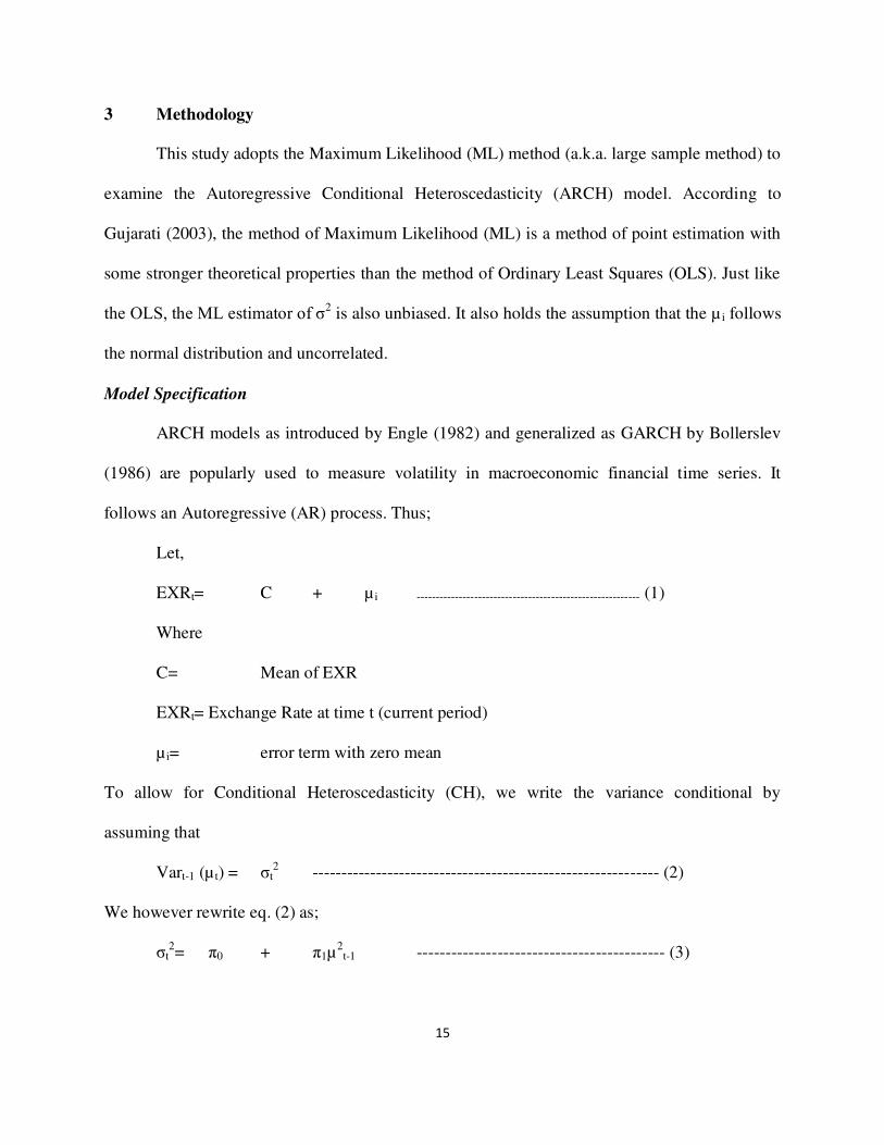
3 Methodology

This study adopts the Maximum Likelihood (ML) method (a.k.a. large sample method) to

examine the Autoregressive Conditional Heteroscedasticity (ARCH) model. According to

Gujarati (2003), the method of Maximum Likelihood (ML) is a method of point estimation with

some stronger theoretical properties than the method of Ordinary Least Squares (OLS). Just like

the OLS, the ML estimator of σ2 is also unbiased. It also holds the assumption that the µ i follows

the normal distribution and uncorrelated.

Model Specification

ARCH models as introduced by Engle (1982) and generalized as GARCH by Bollerslev

(1986) are popularly used to measure volatility in macroeconomic financial time series. It

follows an Autoregressive (AR) process. Thus;

Let,

EXRt= C + µ i ---------------------------------------------------------- (1)

Where

C= Mean of EXR

EXRt= Exchange Rate at time t (current period)

µ i= error term with zero mean

To allow for Conditional Heteroscedasticity (CH), we write the variance conditional by

assuming that

Vart-1 (µ t) = σt2 ------------------------------------------------------------ (2)

We however rewrite eq. (2) as;

σt2= π0 + π1µ

2t-1 ------------------------------------------- (3)

16

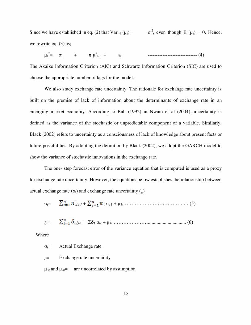
Since we have established in eq. (2) that Vart-1 (µ t) = σt2, even though E (µ t) = 0. Hence,

we rewrite eq. (3) as;

µ t2= π0 + π1µ

2t-1 + εt ------------------------------ (4)

The Akaike Information Criterion (AIC) and Schwartz Information Criterion (SIC) are used to

choose the appropriate number of lags for the model.

We also study exchange rate uncertainty. The rationale for exchange rate uncertainty is

built on the premise of lack of information about the determinants of exchange rate in an

emerging market economy. According to Ball (1992) in Nwani et al (2004), uncertainty is

defined as the variance of the stochastic or unpredictable component of a variable. Similarly,

Black (2002) refers to uncertainty as a consciousness of lack of knowledge about present facts or

future possibilities. By adopting the definition by Black (2002), we adopt the GARCH model to

show the variance of stochastic innovations in the exchange rate.

The one- step forecast error of the variance equation that is computed is used as a proxy

for exchange rate uncertainty. However, the equations below establishes the relationship between

actual exchange rate (σt) and exchange rate uncertainty (¿)

σt= o¿t-1 + 1 σt-1 + µ3t……………………………….… (5)

¿t= 0¿t-I+ Ʃ𝛅1 σt-1+ µ4t …………………............................... (6)

Where

σt = Actual Exchange rate

¿= Exchange rate uncertainty

µ3t and µ4t= are uncorrelated by assumption

17

(4) Empirical Results and Discussion

This section critically presents and analyzes our empirical result based on our method of

analysis as stated in the previous section. As the model (ARCH) suggests, it implies that

heteroscedasticity or unequal variance may have an autoregressive structure such that

heteroscedasticity observed over different periods are uncorrelated.

It is modish (fashionable) to state that, the hunch of ARCH is based on the fact that

financial planning is often difficult due to volatility in financial time series, in this case is the

exchange rate. It is also imperative to state the three basic assumptions that underlie the ARCH

model;

a. Normality (Gaussian) Distribution

b. Students t- distribution

c. Generalize Error Distribution (G.E.D)

The results of our models are presented trenchantly below using statistical tools (tables

and equations);

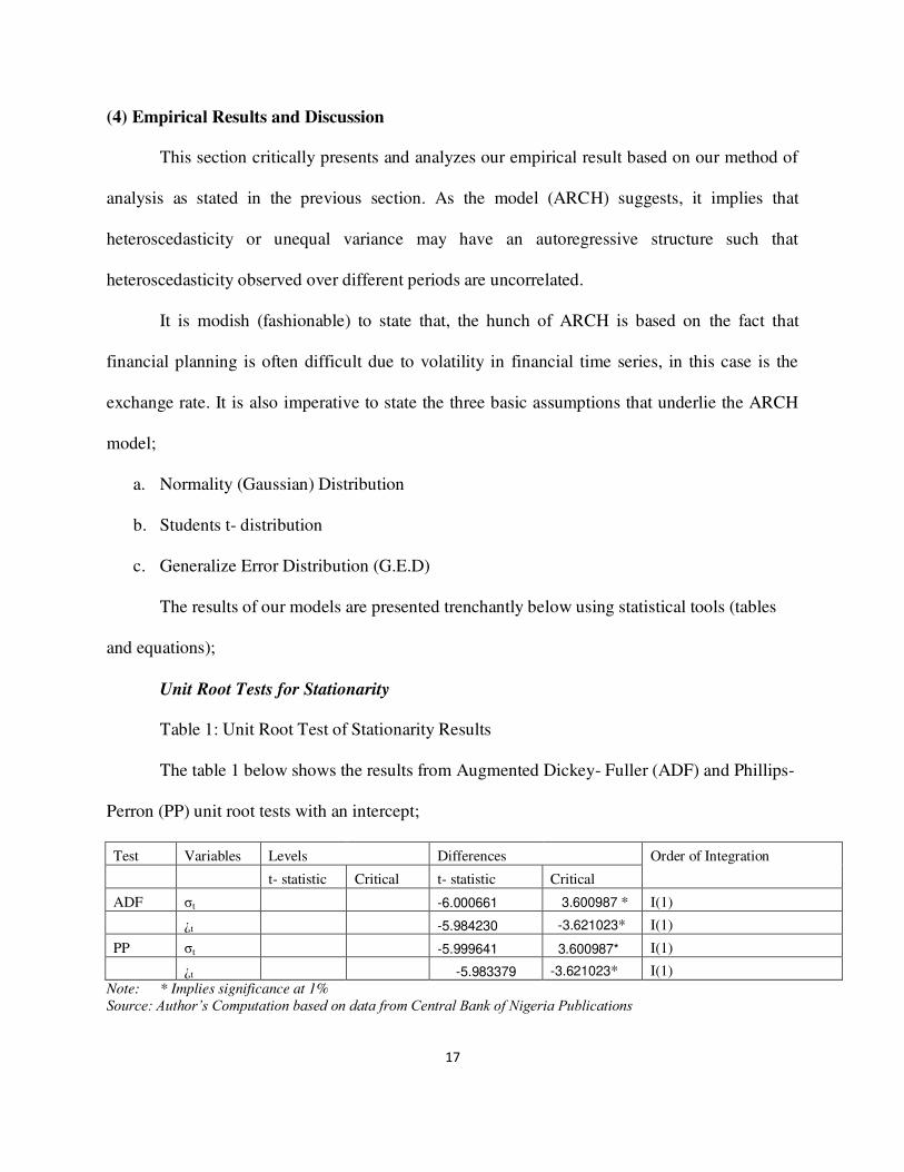
Unit Root Tests for Stationarity

Table 1: Unit Root Test of Stationarity Results

The table 1 below shows the results from Augmented Dickey- Fuller (ADF) and Phillips-

Perron (PP) unit root tests with an intercept;

Test Variables Levels

Differences

Order of Integration

t- statistic Critical t- statistic Critical

ADF σt -6.000661 3.600987 * I(1)

¿t

-5.984230 -3.621023* I(1)

PP σt -5.999641 3.600987* I(1)

¿t

-5.983379 -3.621023* I(1)

Note: * Implies significance at 1% Source: Author’s Computation based on data from Central Bank of Nigeria Publications

18

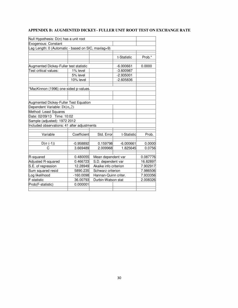
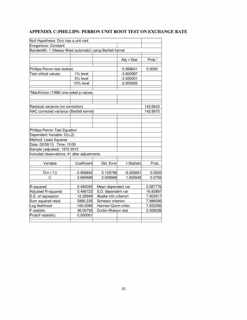
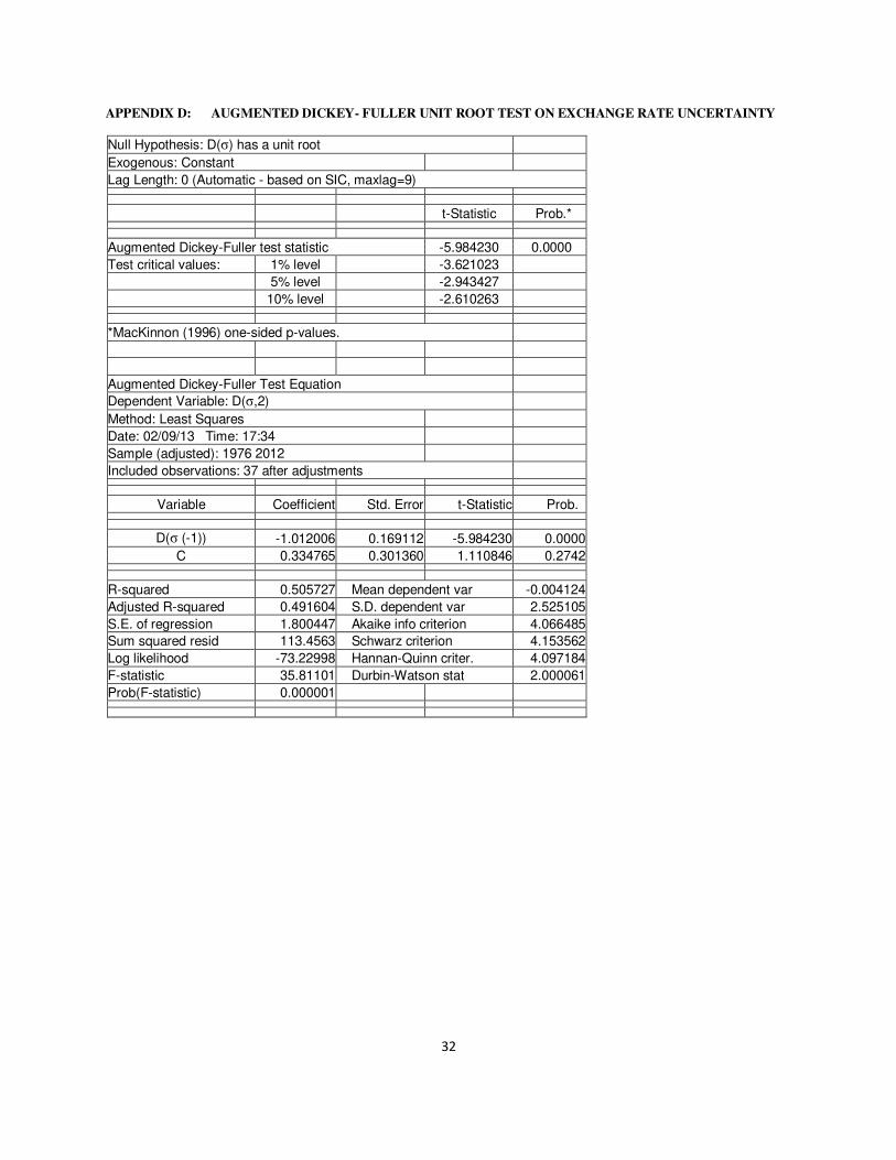
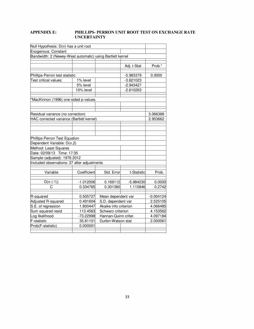
An application of the Augmented Dickey- Fuller (ADF) and Philllips- Perron (PP) tests reported

in table 1 above indicates that the unit root test results show that the actual exchange rate in the

model is integrated of the order one, I(1), implying that they are stationary at their first

difference, also, exchange rate uncertainty is integrated of order one, I(1).

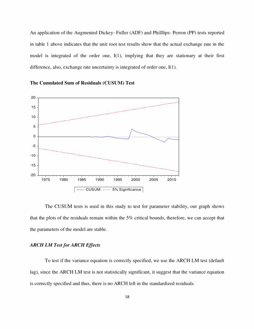
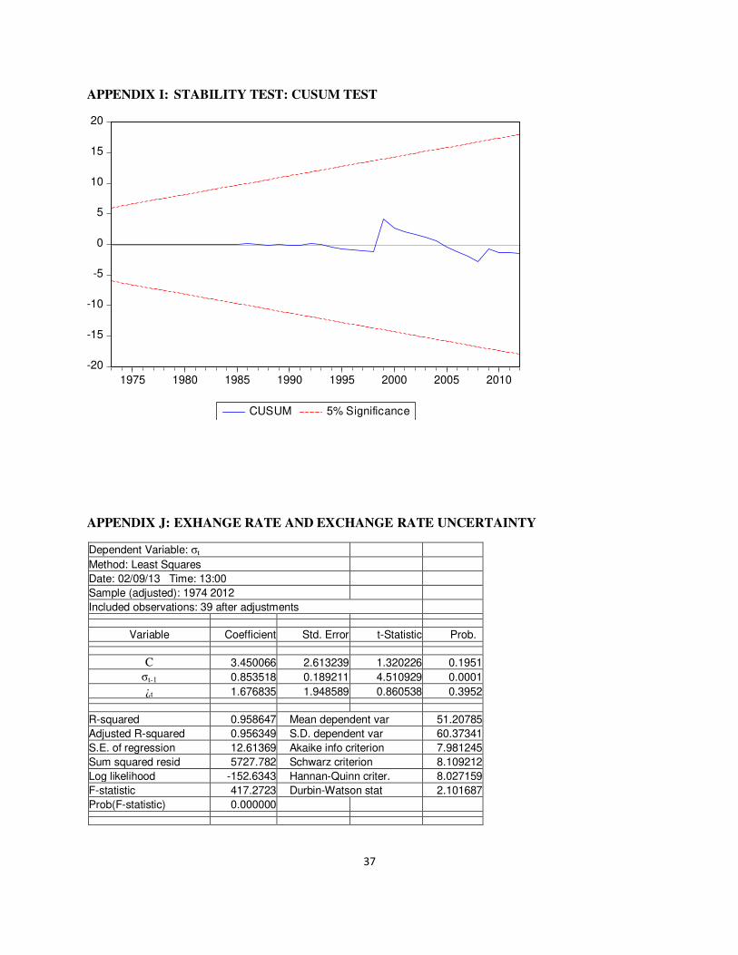
The Cumulated Sum of Residuals (CUSUM) Test

-20

-15

-10

-5

0

5

10

15

20

1975 1980 1985 1990 1995 2000 2005 2010

CUSUM 5% Significance

The CUSUM tests is used in this study to test for parameter stability, our graph shows

that the plots of the residuals remain within the 5% critical bounds, therefore, we can accept that

the parameters of the model are stable.

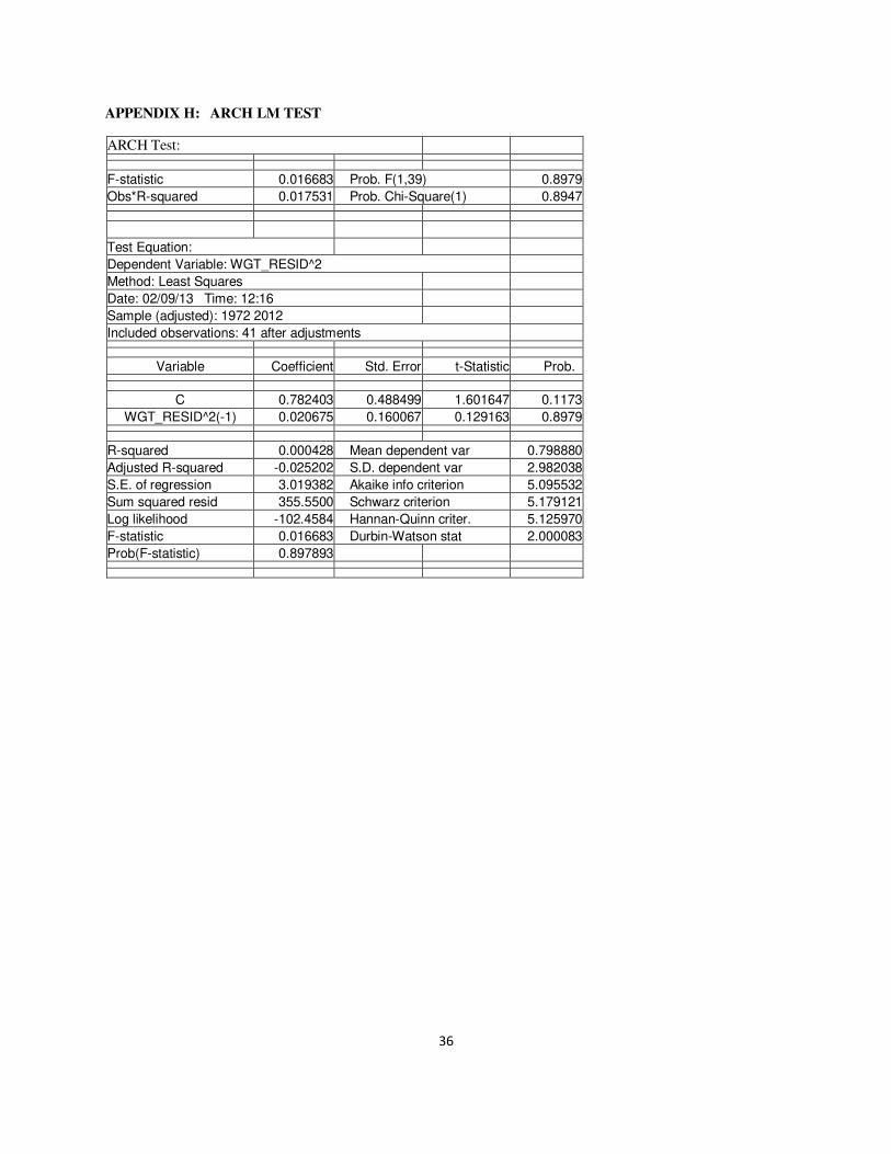
ARCH LM Test for ARCH Effects

To test if the variance equation is correctly specified, we use the ARCH LM test (default

lag), since the ARCH LM test is not statistically significant, it suggest that the variance equation

is correctly specified and thus, there is no ARCH left in the standardized residuals.

19

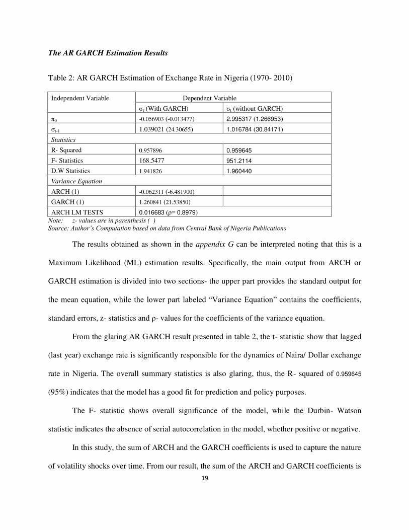
The AR GARCH Estimation Results

Table 2: AR GARCH Estimation of Exchange Rate in Nigeria (1970- 2010)

Independent Variable Dependent Variable

σt (With GARCH) σt (without GARCH)

π0 -0.056903 (-0.013477) 2.995317 (1.266953)

σt-1 1.039021 (24.30655) 1.016784 (30.84171)

Statistics

R- Squared 0.957896 0.959645

F- Statistics 168.5477 951.2114

D.W Statistics 1.941826 1.960440

Variance Equation

ARCH (1) -0.062311 (-6.481900) GARCH (1) 1.260841 (21.53850)

ARCH LM TESTS 0.016683 (ρ= 0.8979)

Note: z- values are in parenthesis ( ) Source: Author’s Computation based on data from Central Bank of Nigeria Publications

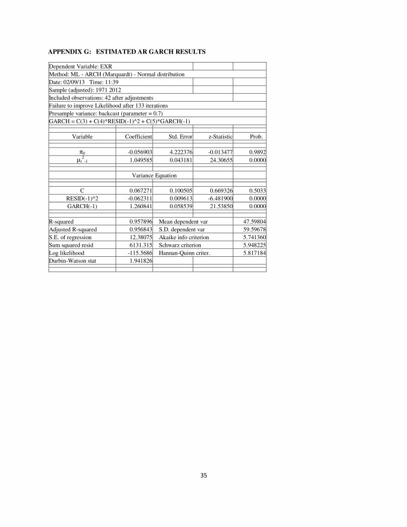
The results obtained as shown in the appendix G can be interpreted noting that this is a

Maximum Likelihood (ML) estimation results. Specifically, the main output from ARCH or

GARCH estimation is divided into two sections- the upper part provides the standard output for

the mean equation, while the lower part labeled “Variance Equation” contains the coefficients,

standard errors, z- statistics and ρ- values for the coefficients of the variance equation.

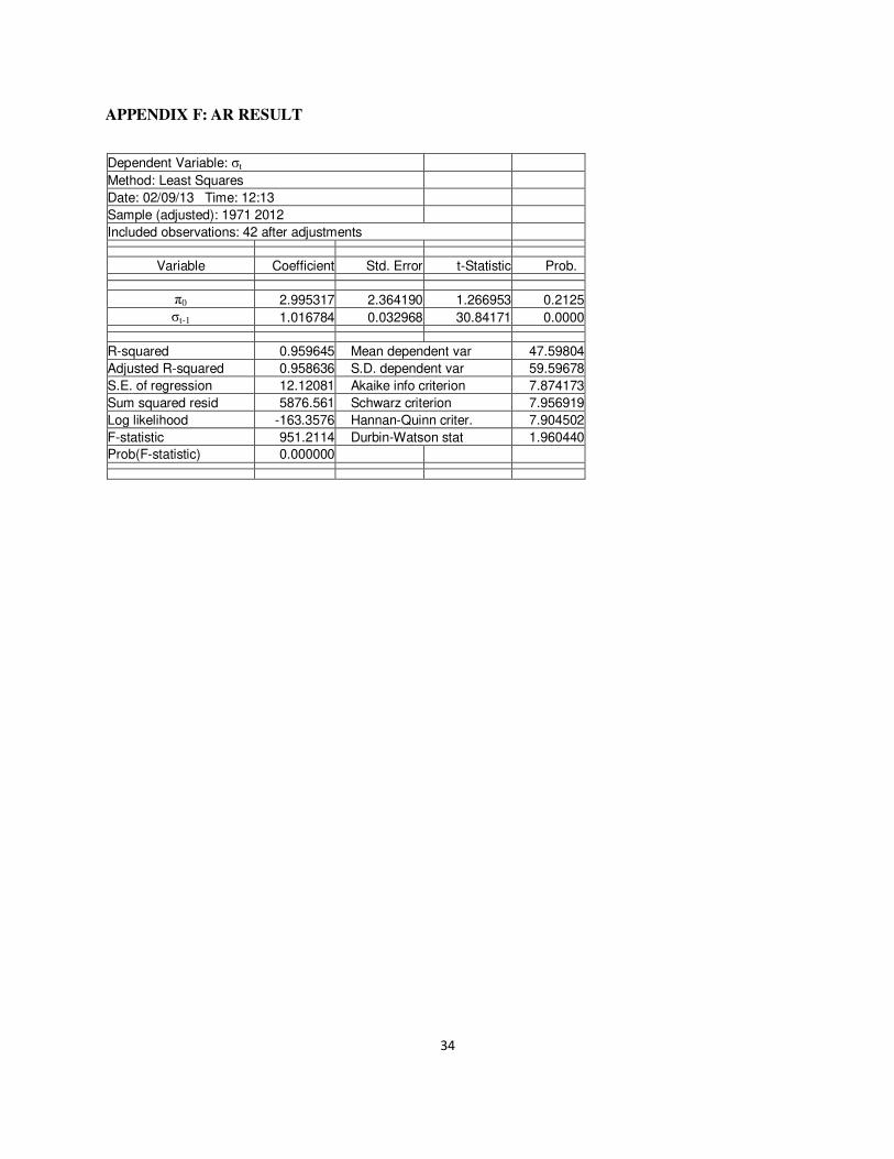
From the glaring AR GARCH result presented in table 2, the t- statistic show that lagged

(last year) exchange rate is significantly responsible for the dynamics of Naira/ Dollar exchange

rate in Nigeria. The overall summary statistics is also glaring, thus, the R- squared of 0.959645

(95%) indicates that the model has a good fit for prediction and policy purposes.

The F- statistic shows overall significance of the model, while the Durbin- Watson

statistic indicates the absence of serial autocorrelation in the model, whether positive or negative.

In this study, the sum of ARCH and the GARCH coefficients is used to capture the nature

of volatility shocks over time. From our result, the sum of the ARCH and GARCH coefficients is

20

not close to unity; this indicates that exchange rate volatility shocks are not quite persistent in

Nigeria.

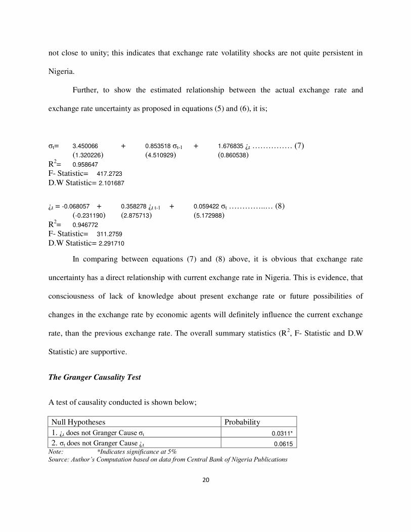
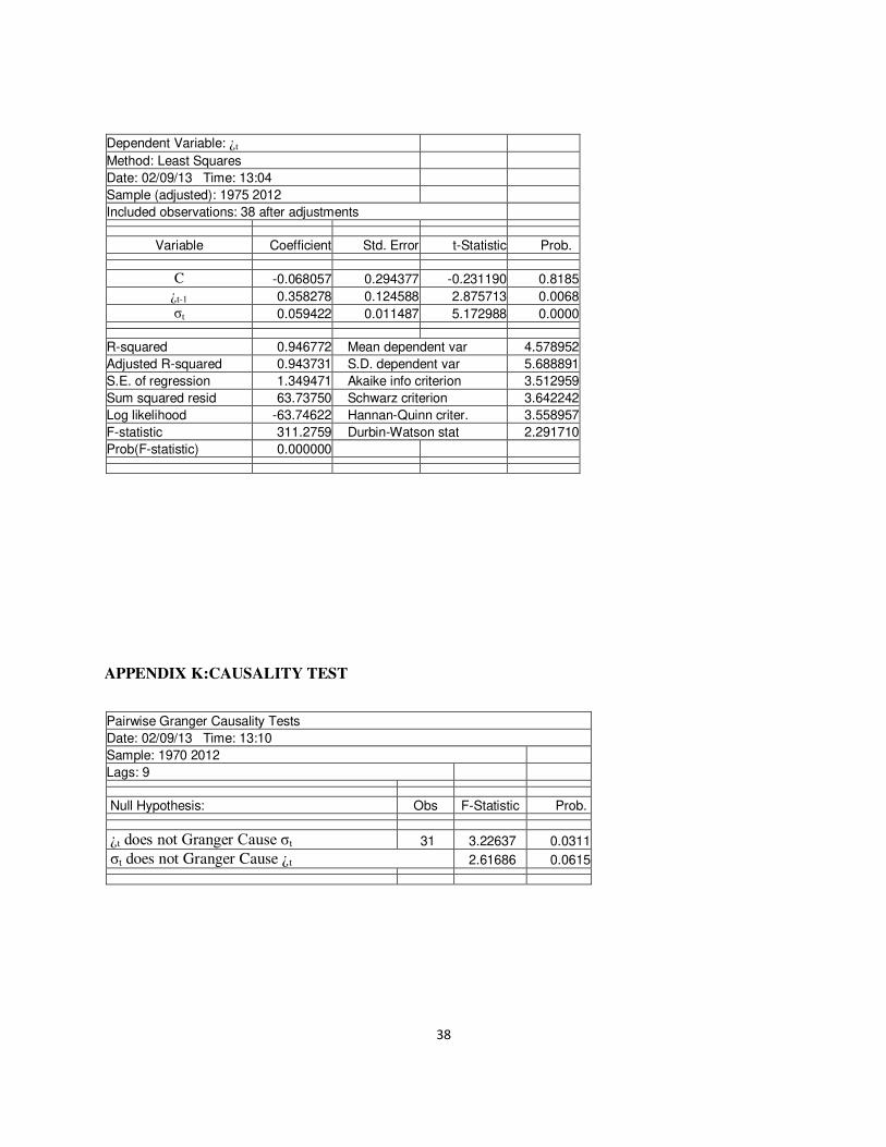
Further, to show the estimated relationship between the actual exchange rate and

exchange rate uncertainty as proposed in equations (5) and (6), it is;

σt= 3.450066 + 0.853518 σt-1 + 1.676835 ¿t …………… (7) (1.320226) (4.510929) (0.860538)

R2= 0.958647

F- Statistic= 417.2723

D.W Statistic= 2.101687

¿t = -0.068057 + 0.358278 ¿t t-1 + 0.059422 σt …………..… (8)

(-0.231190) (2.875713) (5.172988)

R2= 0.946772

F- Statistic= 311.2759

D.W Statistic= 2.291710

In comparing between equations (7) and (8) above, it is obvious that exchange rate

uncertainty has a direct relationship with current exchange rate in Nigeria. This is evidence, that

consciousness of lack of knowledge about present exchange rate or future possibilities of

changes in the exchange rate by economic agents will definitely influence the current exchange

rate, than the previous exchange rate. The overall summary statistics (R2, F- Statistic and D.W

Statistic) are supportive.

The Granger Causality Test

A test of causality conducted is shown below;

Null Hypotheses Probability

1. ¿t does not Granger Cause σt 0.0311*

2. σt does not Granger Cause ¿t 0.0615

Note: *Indicates significance at 5% Source: Author’s Computation based on data from Central Bank of Nigeria Publications

21

We however conclude that exchange rate uncertainty Granger cause exchange rate in

Nigeria. Inotherwords, the results show that the direction of causality is more powerful and

significant from exchange rate uncertainty to actual exchange rate in Nigeria. This finding

supports the results of equation (7) and (8).

5 Summary of Major Findings, Recommendations and Conclusion

In this research, we conduct a closer examination of exchange rate volatility in Nigeria

with respect to both the fixed and flexible exchange rate regime. One of the frequent reasons as

cited in literature for the adoption of flexible exchange rate policy is that it helps to correct

balance of payments imbalances and its ability to accommodate unexpected domestic

fluctuations. However, very few studies offer direct empirical evidence to support this view.

Inorder to capture the exchange rate volatility and the effects of exchange rate

uncertainties that is associated to the actual exchange rate, we employed the maximum likelihood

techniques.

We find evidence from the AR GARCH result that lagged (last year) exchange rate is

significantly responsible for the dynamics of Naira/ Dollar exchange rate in Nigeria. The result

shows that exchange rate volatility shocks are not quite persistent in Nigeria.

We also find that exchange rate uncertainty has a direct relationship with current

exchange rate in Nigeria. Further, the Granger causality test conducted shows that the direction

of causality is more powerful and significant from exchange rate uncertainty to actual exchange

rate in Nigeria.

22

Recommendations

Based on our findings, the following recommendations are made;

1. There should be proper management of exchange rate, to forestall costly distortions in the

Nigerian economy.

2. With hind-sight, nevertheless this study suggests that subsequent researchers should

ascertain the determinants of exchange rate uncertainties.

3. It is plausible to recommend exchange rate targeting to the Nigerian monetary authorities.

4. It is important that monetary authorities ensure transparency in determining exchange rate

process such that various economic distortions associated with exchange rate may be minimized.

Conclusion

Many researchers have argued that unanticipated foreign exchange rate may lead to

balance of trade deficit, and therefore causes disequilibrium which is detrimental to achieving

macroeconomic stabilization objectives. In this paper, we analyze exchange rate volatility in

Nigeria between 1970 and 2010; we find evidence that ceteris paribus lagged exchange rate is

significantly responsible for the dynamics of current exchange rate in Nigeria. This implies that

prior information about exchange rate can be useful to ascertain the exchange rate at current time

period. One clear conclusion which emerged from the granger causality analysis conducted is

that the direction of causality is more powerful and significant from exchange rate uncertainty to

actual exchange rate in Nigeria.

23

References

Adam, C. and Cobham, D. (2008). Alternative exchange rate regimes for MENA countries:

gravity model estimates of the trade effects. Mimeo

Adubi, A.A., and Okunmadewa, F. (1999). Price, exchange rate volatility and Nigeria’s agricultural trade flows: A dynamic analysis. African Economic Research Consortium

(AERC) Research Paper 87

Aikaeli, J. (2007). Money and Inflation Dynamics: A Lag between Change in Money Supply and

the Corresponding Inflation Response in Tanzania. Working Paper Series.

Agiobenebo, T.J. (1999). Introductory Microeconomics: Theory and Applications. Port Harcourt,

Markowitz Centre for Research and Development.

Alaba, O. B. (2003). Exchange Rate Uncertainty and Foreign Direct Investment in Nigeria. A

Paper Presented at the WIDER Conference on Sharing Global Prosperity, Helsinki,

Finland, 6-7 September 2003.

Allayannis, G., Brown, G.W. and Klapper, L.F. (2001). Exchange Rate Risk Management:

Evidence from East Asia. Darden Business School Working Paper No. 01-09

Alvarez-Diaz, M. (2008). A note on forecasting exchange rates using a cluster technique.

International Journal of Business Forecasting and Marketing Intelligence, Vol. 1, No. 1,

pp.68–81.

Avellaneda, M. and Zhu, Y. (1997a). An E-ARCH Model for the Term Structure of Implied

Volatility of FX Options. Working Paper Series available online at http//www.ssrn.com

Bailliu, J., Lafrance, R., and Jean-François Perrault (2002). Does Exchange Rate Policy Matter

for Growth? Bank of Canada Working Paper 2002-17

24

Balogun, E.D. (2007). Effects of exchange rate policy on bilateral export trade of WAMZ

countries. MPRA Paper No. 6234, Available Online at http://mpra.ub.uni-

muenchen.de/6234/

Benigno, G. and Benigno, P. (2000). Monetary Policy Rules and the Exchange Rate. available at

ssrn.com

Bera, A. and Higgins, M. (1993). ARCH Models: Properties, Estimation and Testing. Journal of

Economic Surveys, vol. 7, pp. 305- 366.

Bhattarai, K.R. and Mark K. Armah, M.K. (2005). The Effects of Exchange Rate on the Trade

Balance in Ghana: Evidence from Cointegration Analysis. Research Memorandum 52

Bitzenis, A. and Marangos, J. (2007). The monetary model of exchange rate determination: the

case of Greece (1974–1994). International Journal of. Monetary Economics and Finance,

Vol. 1, No. 1, pp. 57- 88

Black, J. (2003). Oxford Dictionary of Economics. New York, Oxford University Press.

Bleaney, M. and Fielding, D. (1999). Exchange Rate Regimes, Inflation and Output Volatility in

Developing Countries. Centre for Research in Economic Development and International

Trade (CREDIT) Research Paper 99/4

Bleaney, M. and Francisco, M. (2007). The Performance of Exchange Rate Regimes in

Developing Countries – Does the Classification Scheme Matter? Centre for Research in

Economic Development and International Trade (CREDIT) Research Paper, No. 07/04

Bollerslev, T., Engle, R. and Nelson, D. (1994). ARCH Models,” Vol. IV, Elsvier Science,

Chapter Handbook in Econometrics, Pp. 2961- 3038

25

Bollerslev, T. (1986). Generalized Autoregressive Conditional Heteroscedasticity. Journal of

Econometrics, Vol. 31, pp. 307-326.

Bollerslev, T. (1990). Modelling the Coherence in Short Run Nominal Exchange Rates: A

Multivariate Generalized ARCH Model. Review of Economics and Statistics 72, 498-

505.

Bouakez, H., Kano, T. and Xu, J. (2007). Imperfect Information, Learning, and Exchange Rate

Dynamics. Social Sciences and Humanities Research Council

Busse, M., Hefeker, C. and Koopmann, G. (2004). Between Two Poles: Matching Trade and

Exchange Rate Regimes in Mercosur. Hamburg Institute of International Economics

(HWWA) Discussion Paper 301

Canetti, E. and Greene, J. (1991). Monetary growth and exchange rate depreciation as causes of

inflation in African countries. Centre For Economic Research on Africa (CERAF)

Caporale, G. M. Cipollini, A. and Demetriades, P. (2003). Monetary Policy and the Exchange

Rate During the Asian Crisis: Identification Through Heteroscedasticity. CEIS Tor

Vergata - Research Paper Series No. 23.

Chen, Y., Rogoff, K. and Rossi, B. (2008). Can Exchange Rates Forecast Commodity Prices?

University of Washington Working Paper

Cheng, K. C. (2007). A VAR Analysis of Kenya's Monetary Policy Transmission Mechanism:

How Does the Central Bank's Repo Rate Affect the Economy? IMF Working Paper No.

06/300.

Chukwuma, A. (2002). Real Exchange Rate Distortions and External Balance Position of

Nigeria: Issues and Policy Options. Paper submitted for publication to the Journal of

African Finance and Economic Development, Institute of African American Affairs, New

York University.

26

Coricelli, F. and Jazbec, B. (2001). Real Exchange Rate Dynamics in Transition Economies.

CEPR Discussion Paper No. 2869, Available online at

www.cepr.org/pubs/dps/DP2869.asp

Dufrenot, G.J. and Yehoue, E.B. (2005). Real Exchange Rate Misalignment: A Panel Co-

Integration and Common Factor Analysis. IMF Working Paper WP/05/164

Engle, R.F. (1982). Autoregressive Conditional Heteroscedasticity with estimates of the variance

of UK inflation. Econometrica 50, 987-1008

Engle, R.F. (2000). Dynamic Conditional Correlation - A Simple Class of Multivariate GARCH

Models. UCSD Economics Discussion Paper No. 2000-09

Engle, R.F. (2001). GARCH 101: An Introduction to the Use of ARCH/GARCH Models in

Applied Econometrics. NYU Working Paper No. FIN-01-030

Esquivel, G. and Larraín, F.B. (2002). The Impact of G-3 Exchange Rate Volatility on

Developing Countries. UNCTAD/GDS/MDPB/G24/16 G-24 Discussion Paper Series,

No. 16,

Gbanador, C.A. (2007). Modern Macroeconomics. Port Harcourt, Pearl Publishers

Goldstein, M. (2004). Adjusting China's Exchange Rate Policies. Institute for International

Economics Working Paper No. 04-1

Grauwe, P.D. (1988). The Long- Swings in Real Exchange Rates- Do they fit into Our Theories?

BOJ Monetary and Economic Studies, Vol. 6, No. 1, May 1988.

27

Gupta, J. P., Chevalier, A. and Sayekt, F. (2000). The Causality between Interest Rate, Exchange

Rate and Stock Price in Emerging Markets: The Case of the Jakarta Stock Exchange.

EFMA 2000 Athens

Greene, W. H. (2000). Econometric Analysis. 4th ed., Prentice Hall, New Jersey.

Gylfason, T. (2002). The Real Exchange Rate Always Floats. Australian Economic Papers.

Hansen, P.R. and Lunde, A. (2004). A Forecast Comparison of Volatility Models: Does

Anything Beat a GARCH (1, 1)? Brown Univ. Economics Working Paper No. 01-04

Harvey, A. (1990). The Econometric Analysis of Time Series. the MIT Press, Cambridge.

Hondroyiannis, G., Swamy, P.A.V.B., Tavlas, G., Ulan, M. (2005). Some Further Evidence on

Exchange-Rate Volatility and Exports. Bank of Greece Working Paper No. 28 October

2005

Hooper, P. and Kohlhagen, S. W. (1976). The Effect of Exchange Rate Uncertainty on the Prices

and Volume of International Trade. International Finance Discussion Papers, November

1976, No. 91

Jarmuzek, M., Orlowski, L. T. and Radziwill, A. (2004). Monetary Policy Transparency in the

Inflation Targeting Countries: The Czech Republic, Hungary and Poland. Center for

Social and Economic Research Studies and Analyses Working Paper No. 281.

Jhingan, M.L. (2005). The Economics of Development and Planning. 38th edition, Delhi, Vrinda

Publications (P) Ltd.

28

Joshi, V. (2003). Financial Globalisation, Exchange Rates and Capital Controls in Developing

Countries. Conference organized by the Re-inventing Bretton Woods Committee,

Madrid, 13-14 May.

Kellard, N. and Sarantis, N. (2007). Can Exchange Rate Volatility Explain Persistence in the

Forward Premium? School of Accounting, Finance and Management, Essex Finance

Centre, Discussion Paper No DP 07/06

Kidane, A. (1999). Real exchange rate price and agricultural supply response in Ethiopia: The

case of perennial crops. African Economic Research Consortium (AERC) Research Paper

99

Kuijs, L. (1998). Determinants of Inflation, Exchange rate, and output in Nigeria. IMF Working

Paper

Mandelbrot, B.B., Fisher, A.J. and Calvet, L.E. (1997a). A Multifractal Model of Asset Returns.

Cowles Foundation Discussion Paper No. 1164

Mandelbrot, B.B., Fisher, A.J. and Calvet, L.E. (1997b). “Multifractality of Deutschemark / US

Dollar Exchange Rates. Cowles Foundation Discussion Paper No. 1166

Nabli, M.K. (2002). Exchange Rate Regime and Competitiveness of Manufactured Exports: The

Case of MENA Countries. Available online

Nkurunziza, J.D. (2002). Exchange rate policy and the parallel market for foreign currency in

Burundi. AERC Research Paper 123

Nwafor, F.C. (2006). The Naira-Dollar Exchange Rate Determination: A Monetary. International

Research Journal of Finance and Economics, ISSN 1450-2887 Issue 5, Euro Journals

Publishing, Inc., Available at http://www.eurojournals.com/finance.htm

29

Ruiz, I.C. (2005). Empirical analysis on the real effects of inflation and exchange rate

uncertainty: The case of Colombia. Ecos de Economía No. 20. Medellín, abril 2005, pp. 7

- 28

Rutasitara, L. (2004). Exchange rate regimes and inflation in Tanzania. AERC Research Paper

138

Tenreyro, S. (2006). On the Trade Impact of Nominal Exchange Rate Volatility. London School

of Economics.

Velasco, A. (2000). Exchange -Rate Policies For Developing Countries: What Have We

Learned? What Do We Still Not Know? United Nations Conference on Trade and

Development UNCTAD/GDS/MDPB/G24/5, G-24 Discussion Paper Series

Wang, K. and Barrett, C.B. (2007). Estimating the Effects of Exchange Rate Volatility on Export

Volumes. Forthcoming in Journal of Agricultural and Resource Economics

Weeks, J. (2008). The effectiveness of monetary Policy reconsidered. International Poverty

Centre United Nations Development Programme, Technical Paper, available online at

http://www.undp-povertycentre.org

Yeyati, E.L. and Sturzenegger, F. (1999). Classifying Exchange Rate Regimes: Deeds vs. Words.

available online at http://www.utdt.edu/~fsturzen or http://www.utdt.edu/~ely

http://www.undp-povertycentre.org/

30

APPENDIX B: AUGMENTED DICKEY- FULLER UNIT ROOT TEST ON EXCHANGE RATE

Null Hypothesis: D(σ) has a unit root

Exogenous: Constant

Lag Length: 0 (Automatic - based on SIC, maxlag=9) t-Statistic Prob.*

Augmented Dickey-Fuller test statistic -6.000661 0.0000

Test critical values: 1% level -3.600987

5% level -2.935001

10% level -2.605836

*MacKinnon (1996) one-sided p-values.

Augmented Dickey-Fuller Test Equation

Dependent Variable: D((σt,2)

Method: Least Squares

Date: 02/09/13 Time: 10:02

Sample (adjusted): 1972 2012

Included observations: 41 after adjustments

Variable Coefficient Std. Error t-Statistic Prob.

D(σ (-1)) -0.958892 0.159798 -6.000661 0.0000

C 3.669489 2.009968 1.825645 0.0756

R-squared 0.480055 Mean dependent var 0.087776

Adjusted R-squared 0.466723 S.D. dependent var 16.82897

S.E. of regression 12.28949 Akaike info criterion 7.902917

Sum squared resid 5890.235 Schwarz criterion 7.986506

Log likelihood -160.0098 Hannan-Quinn criter. 7.933356

F-statistic 36.00793 Durbin-Watson stat 2.008326

Prob(F-statistic) 0.000001

31

APPENDIX C: PHILLIPS- PERRON UNIT ROOT TEST ON EXCHANGE RATE


Exogenous: Constant

Bandwidth: 1 (Newey-West automatic) using Bartlett kernel Adj. t-Stat Prob.*

Phillips-Perron test statistic -5.999641 0.0000


5% level -2.935001

10% level -2.605836


Residual variance (no correction) 143.6643

HAC corrected variance (Bartlett kernel) 142.8975

Phillips-Perron Test Equation

Dependent Variable: D(σ,2)


Date: 02/09/13 Time: 10:05




D(σ (-1)) -0.958892 0.159798 -6.000661 0.0000

C 3.669489 2.009968 1.825645 0.0756








32

APPENDIX D: AUGMENTED DICKEY- FULLER UNIT ROOT TEST ON EXCHANGE RATE UNCERTAINTY


Exogenous: Constant

Lag Length: 0 (Automatic - based on SIC, maxlag=9) t-Statistic Prob.*

Augmented Dickey-Fuller test statistic -5.984230 0.0000


5% level -2.943427

10% level -2.610263


Augmented Dickey-Fuller Test Equation



Date: 02/09/13 Time: 17:34




D(σ (-1)) -1.012006 0.169112 -5.984230 0.0000

C 0.334765 0.301360 1.110846 0.2742

R-squared 0.505727 Mean dependent var -0.004124







33

APPENDIX E: PHILLIPS- PERRON UNIT ROOT TEST ON EXCHANGE RATE

UNCERTAINTY


Exogenous: Constant

Bandwidth: 2 (Newey-West automatic) using Bartlett kernel Adj. t-Stat Prob.*

Phillips-Perron test statistic -5.983379 0.0000


5% level -2.943427

10% level -2.610263


Residual variance (no correction) 3.066388

HAC corrected variance (Bartlett kernel) 2.953662

Phillips-Perron Test Equation



Date: 02/09/13 Time: 17:35




D(σ (-1)) -1.012006 0.169112 -5.984230 0.0000

C 0.334765 0.301360 1.110846 0.2742

R-squared 0.505727 Mean dependent var -0.004124







34

APPENDIX F: AR RESULT

Dependent Variable: σt


Date: 02/09/13 Time: 12:13




π0 2.995317 2.364190 1.266953 0.2125

σt-1 1.016784 0.032968 30.84171 0.0000








35

APPENDIX G: ESTIMATED AR GARCH RESULTS

Dependent Variable: EXR

Method: ML - ARCH (Marquardt) - Normal distribution

Date: 02/09/13 Time: 11:39



Failure to improve Likelihood after 133 iterations

Presample variance: backcast (parameter = 0.7)

GARCH = C(3) + C(4)*RESID(-1)^2 + C(5)*GARCH(-1)

Variable Coefficient Std. Error z-Statistic Prob.

π0 -0.056903 4.222376 -0.013477 0.9892

µt2

-1 1.049585 0.043181 24.30655 0.0000

Variance Equation

C 0.067271 0.100505 0.669326 0.5033

RESID(-1)^2 -0.062311 0.009613 -6.481900 0.0000

GARCH(-1) 1.260841 0.058539 21.53850 0.0000






Durbin-Watson stat 1.941826

36

APPENDIX H: ARCH LM TEST

ARCH Test:

F-statistic 0.016683 Prob. F(1,39) 0.8979

Obs*R-squared 0.017531 Prob. Chi-Square(1) 0.8947

Test Equation:

Dependent Variable: WGT_RESID^2


Date: 02/09/13 Time: 12:16




C 0.782403 0.488499 1.601647 0.1173

WGT_RESID^2(-1) 0.020675 0.160067 0.129163 0.8979


Adjusted R-squared -0.025202 S.D. dependent var 2.982038






37

APPENDIX I: STABILITY TEST: CUSUM TEST

-20

-15

-10

-5

0

5

10

15

20

1975 1980 1985 1990 1995 2000 2005 2010

CUSUM 5% Significance

APPENDIX J: EXHANGE RATE AND EXCHANGE RATE UNCERTAINTY

Dependent Variable: σt


Date: 02/09/13 Time: 13:00




C 3.450066 2.613239 1.320226 0.1951

σt-1 0.853518 0.189211 4.510929 0.0001

¿t 1.676835 1.948589 0.860538 0.3952








38

Dependent Variable: ¿t


Date: 02/09/13 Time: 13:04




C -0.068057 0.294377 -0.231190 0.8185

¿t-1 0.358278 0.124588 2.875713 0.0068

σt 0.059422 0.011487 5.172988 0.0000








APPENDIX K: CAUSALITY TEST

Pairwise Granger Causality Tests

Date: 02/09/13 Time: 13:10

Sample: 1970 2012

Lags: 9

Null Hypothesis: Obs F-Statistic Prob.

¿t does not Granger Cause σt 31 3.22637 0.0311

σt does not Granger Cause ¿t 2.61686 0.0615

Documents

Exchange rate volatility and exchange rate …Munich Personal RePEc Archive Exchange rate volatility and exchange rate uncertainty in Nigeria: a ﬁnancial econometric analysis (1970-