Ex p eri menta l D es i g n f o r U n i t a n d C l u s ter R a n d o mi d Tri a l s∗

Guido W. Imbens†

June 2011

∗.†Department of Economics, Harvard University, M-24 Littauer Center, Cam-

bridge, MA 02138, and NBER. Electronic correspondence: imbens@harvard.edu,http://www.economics.harvard.edu/faculty/imbens/imbens.html.

1 Introduction

In these notes I discuss the the benefits and disadvantages of stratification and pairing relative

to complete randomization in experiments with randomization at the individual (unit) as well

as at the cluster or group level. The first design I consider is complete randomization, where the

full sample is randomly divided into two subsamples, with all members of the first subsample

assigned to the treatment and all members of the second subsample are assigned to the control

group. The second design I consider is stratified randomization. First the full sample is divided

into subsamples on the basis of covariate values, so that the subsamples are more homogenous

in terms of these covariates than the full sample. For example, one may divide the sample

into subsamples by sex. Within each of the subsamples a completely randomized experiment

is conducted. The third design is pairwise randomization, where the full sample is divided

into pairs, again on the basis of covariate values, and within each pair one member is selected

randomly to be assigned to the treatment group and the other member of the pair is assigned to

the control group. Thus, a pairwise randomized experiment can be viewed as a special case of a

stratified randomized experiment where each strata consists of exactly two units, one for each

level of the treatment. To simplify the exposition, whenever I refer to stratified randomized

experiments, it should be interpreted as a reference to experiments with at least two units for

each treatment in each stratum. All the issues discussed in these notes also arise in settings

with more than two treatment levels, but for ease of exposition I will focus on the case with

two treatment levels.

There is some confusion in the literature regarding the relative merits of the various levels

of randomization, and conflicting recommendations. Some researchers recommend pairwise

randomization in all cases. Others favor in all cases stratified randomization (that is, more

than two units per strata). A third group of researchers argues that the preferred strategy

varies, depending on the sample size and the correlation between covariates and outcomes in

the particular study. The latter group is concerned with the degrees of freedom adjustment

if the randomization takes place within strata or pairs, and whether the cost in terms of the

degrees of freedom adjustment outweighs the gain in precision and power from adjusting by

design for part of the heterogeneity between sampling units.

The main conclusions in these notes can be summarized as follows:

1. In experiments with randomization at the unit-level, stratification is superior

to complete randomization, and pairing is superior to stratification in terms

of precision of estimation.

2. Relative to stratification with multiple units in each treatment group in each

stratum, pairing with only a single unit in each treatment group in each

stratum creates analytic complications. Specifically pairing makes it difficult

to consistently estimate the variance of the estimator of the average effect of

the intervention conditional on the covariates, even in large samples, if there

is heterogeneity in the causal effects by covariates. It also makes it difficult

to establish the presence, and estimate the amount, of heterogeneity in the

[1]

average causal effects by covariates.

3. Randomization at the cluster level does not change these conclusions. Ran-

domization at the cluster level creates finite sample complications separate

from the choice of design. These complications are related to the weights the

clusters receive in the estimand of interest .

4. It is particularly helpful to stratify or pair based on cluster size if (i) cluster

size varies substantially, (ii) interest is in average effects for the entire popu-

lation and (iii) cluster size is potentially correlated with the average effect of

the intervention by cluster.

5. The overall recommendation, irrespective of the sample size and correlation

between covariates and outcomes, is to use stratified randomization with rel-

atively many and relatively small strata (to capture as much as possible of

the precision gain from stratification), rather than either complete random-

ization or paired randomization (which would capture all of the potential gain

in precision, but at the price of the analytical complications).

In the rest of these notes I will provide support for these recommendations. I will also

discuss why these recommendations differ from some of the recommendations in the literature.

Most of the discussion will be relatively informal, although some of the arguments need some

formality to clarify the differences between the recommendations in the literature.

Let me make two final introductory comments. The first comment concerns the questions

of interest. Broadly speaking researchers are interested in two types of questions. The first

question concerns point estimation of the average or some other typical effect of the treatment.

I will largely focus on estimation of average effects, and presume that the criterion is to choose

design strategies that minimize, in expectation, the squared difference between the estimator

and the true average effect of the treatment. The second type of question concerns the presence

of any effects of the treatment. Here researchers carry out statistical tests of the null hypothesis

of no effect of the treatment. In that case the criterion for choosing designs strategies is to

maximize power against interesting alternatives to the null hypothesis. Typically the most

interesting alternative that can be used to compare power is a non-zero additive effect of the

treatment. Despite the fact that these two questions are conceptually distinct, in many analyses

they are confounded. A typical scenario is that researchers obtain point estimates of the average

effect, estimate standard errors, and use the associated t-statistic (the ratio of the point estimate

and the estimated standard error) to test for the presence of effects. I suspect that part of the

reason for combining the two questions in one analysis is that although researchers often claim

that they are interested in testing for the presence of causal effects, they may not actually

be that interested in that specific question. If one were to report to policy makers only that

one has concluded at high levels of statistical significance, that the program has some effect,

without being able to articulate the nature of the causal effect (positive or negative on average,

or merely changing the dispersion of the outcome), policy makers would unlikely be satisfied or

[2]

interested. Nevertheless, conceptually it is useful to keep the two questions separate, and use

different strategies for both of them as I will discuss later.

The second comment concerns the estimand in the case where researchers are interested

in the average effect of the treatment. First of all, in many cases the effect of the treatment

is heterogenous. In that case it is important to clarify which average effect is the focus of

the analysis, whether we want the average for our sample, or the average for a population

where our sample can be viewed as a random sample from that population. These questions

generally matter little for estimation, but them matter in important ways for inference and for

comparisons of designs, and because of that, they help clarify the different views concerning

optimal designs in the literature.

In the next section I will discuss some of the comments in the literature regarding the merits

of pairing and stratification. Then, in Sections 3-8 I will discuss issues regarding stratification

and pairing in randomized experiments where the randomization takes place at the unit level.

Next, in Section 9 I discuss issues related to estimands that are weighted average treatment

effects. In Section 10 I discuss additional issues that arise when the randomization is at a

more aggregate (cluster) level. In this discussion most the focus is on illustrative cases with

a single covariate, often taking on just a few values. General implications will be pointed out

throughout the discussion without formal proofs.

2 Views on Stratification in the Literature

It is well known, and without controversy, that in experiments with randomization at the indi-

vidual or unit level, stratification on covariates is beneficial if these covariates are substantially

correlated with the outcome. However, there is less agreement in the literature concerning the

benefits of stratification in small samples if this correlation is potentially weak. Bruhn and

McKenzie (2007) document this in a survey of researchers in development economics, but the

confusion is also apparent in the general applied statistics literature. For example, Snedecor

and Cochran (1989, page 101) write:

“If the criterion [the covariate used for constructing the pairs] has no correlation

with the response variable, a small loss in accuracy results from the pairing due to

the adjustment for degrees of freedom. A substantial loss may even occur if the

criterion is badly chosen so that member of a pair are negatively correlated.”

Box, Hunter and Hunter (2005, page 93) also suggest that there is a tradeoff in terms of accuracy

or variance in the decision to pair, writing:

“Thus you would gain from the paired design only if the reduction in variance from

pairing outweighed the effect of the decrease in the number of degrees of freedom of

the t distribution.”

Klar and Donner (1997) acknowledge these power concerns, but raise additional issues that

make them concerned about pairwise randomized experiments (in the context of randomization

at the cluster level):

[3]

“We shown in this paper that there are also several analytic limitations associated

with pair-matched designs. These include: the restriction of prediction models to

cluster-level baseline risk factors (for example, cluster size), the inability to test for

homogeneity of odds ratios, and difficulties in estimating the intracluster correlation

coefficient. These limitations lead us to present arguments that favour stratified

designs in which there are more than two clusters in each stratum.”

Imai, King and Nall (2009) claim there are no tradeoffs at all between pairing and complete

randomization, and summarily dismiss all claims in the literature to the contrary:

“Claims in the literature about problems with matched-pair cluster randomization

designs are misguided: clusters should be paired prior to randomization when con-

sidered from the perspective of efficiency, power, bias, or robustness.”

and then exhort researchers to randomize matched pairs.

“randomization by cluster without prior construction of matched pairs, when pairing

is feasible, is an exercise in selfdestruction.”

The comments regarding the relative merits of complete randomization, stratification, and

pairwise randomization can be divided into three strands. The first concerns precision of point

estimates. The second argument focuses on statistical power of tests of the null hypothesis

of no effects. The third refers to the statistical limitations regarding the analysis of pairwise

randomized experiments. I will address each of these issues. In summary, the precision of

experiments can be ranked unambiguously, with pairedwise randomization superior to stratifi-

cation, and stratification superior to complete randomization. The standard argument against

pairing and stratification concerning potential loss of power in small samples if covariates are

only weakly correlated with outcomes refer to particular tests, and do not hold generally. Third,

the statistical limitations Klar and Donner (1997) raise are real, and lead me to agree with their

argument against pairwise randomization in favor of stratification.

The argument that pairing leads to a reduction in accuracy is somewhat counterintuitive:

if one constructs pairs based on a covariate that is completely independent of the potential

outcomes, then pairing is for all intents and purposes equivalent to complete randomization.

In these notes I will argue that this intuition is correct and that in fact there is no tradeoff.

I will show that in terms of expected-squared-error, stratification (with the same treatment

probabilities in each stratum) cannot be worse than complete randomization, even in small

samples, and even with little or even no correlation between covariates and outcomes. Ex ante,

committing to stratification can only improve precision, not lower it. Pairing, as the limit of

stratification to the case with only two units per strata, is by that argument at least as good

as any coarser stratification.

There is an important qualification to this claim of superiority of stratification. First, ex

post, given the values of the covariates in the sample, a particular stratification may be inferior

to complete randomization. However, there is no way to exploit this, and it should therefore not

serve as an argument not to stratify ex ante. Formally, the result requires that the sample can be

[4]

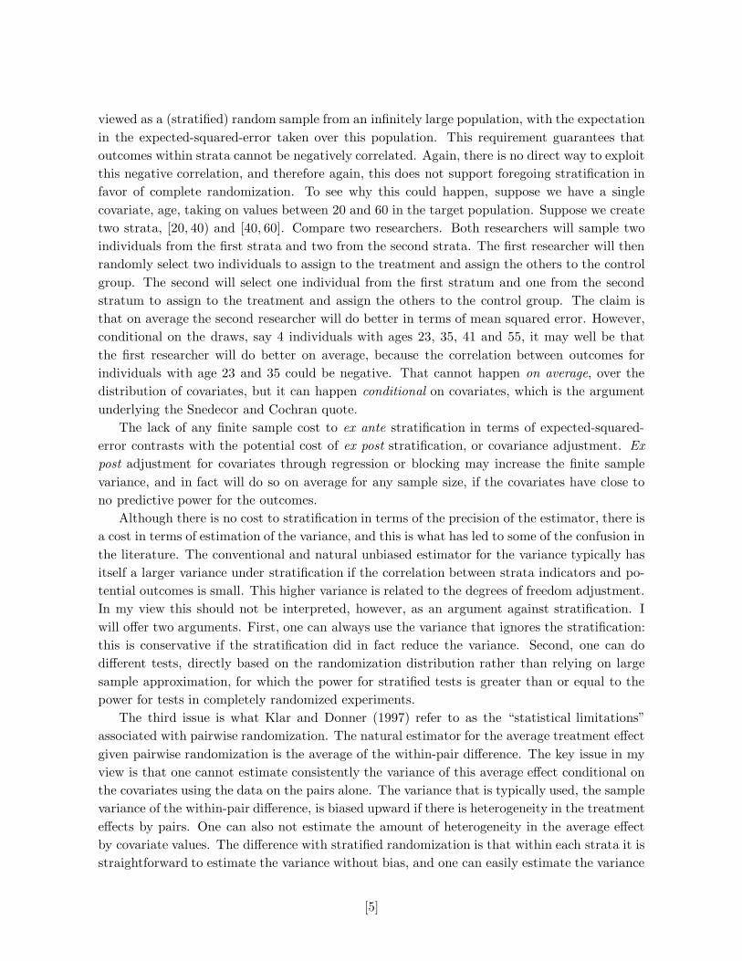
viewed as a (stratified) random sample from an infinitely large population, with the expectation

in the expected-squared-error taken over this population. This requirement guarantees that

outcomes within strata cannot be negatively correlated. Again, there is no direct way to exploit

this negative correlation, and therefore again, this does not support foregoing stratification in

favor of complete randomization. To see why this could happen, suppose we have a single

covariate, age, taking on values between 20 and 60 in the target population. Suppose we create

two strata, [20, 40) and [40, 60]. Compare two researchers. Both researchers will sample two

individuals from the first strata and two from the second strata. The first researcher will then

randomly select two individuals to assign to the treatment and assign the others to the control

group. The second will select one individual from the first stratum and one from the second

stratum to assign to the treatment and assign the others to the control group. The claim is

that on average the second researcher will do better in terms of mean squared error. However,

conditional on the draws, say 4 individuals with ages 23, 35, 41 and 55, it may well be that

the first researcher will do better on average, because the correlation between outcomes for

individuals with age 23 and 35 could be negative. That cannot happen on average, over the

distribution of covariates, but it can happen conditional on covariates, which is the argument

underlying the Snedecor and Cochran quote.

The lack of any finite sample cost to ex ante stratification in terms of expected-squared-

error contrasts with the potential cost of ex post stratification, or covariance adjustment. Ex

post adjustment for covariates through regression or blocking may increase the finite sample

variance, and in fact will do so on average for any sample size, if the covariates have close to

no predictive power for the outcomes.

Although there is no cost to stratification in terms of the precision of the estimator, there is

a cost in terms of estimation of the variance, and this is what has led to some of the confusion in

the literature. The conventional and natural unbiased estimator for the variance typically has

itself a larger variance under stratification if the correlation between strata indicators and po-

tential outcomes is small. This higher variance is related to the degrees of freedom adjustment.

In my view this should not be interpreted, however, as an argument against stratification. I

will offer two arguments. First, one can always use the variance that ignores the stratification:

this is conservative if the stratification did in fact reduce the variance. Second, one can do

different tests, directly based on the randomization distribution rather than relying on large

sample approximation, for which the power for stratified tests is greater than or equal to the

power for tests in completely randomized experiments.

The third issue is what Klar and Donner (1997) refer to as the “statistical limitations”

associated with pairwise randomization. The natural estimator for the average treatment effect

given pairwise randomization is the average of the within-pair difference. The key issue in my

view is that one cannot estimate consistently the variance of this average effect conditional on

the covariates using the data on the pairs alone. The variance that is typically used, the sample

variance of the within-pair difference, is biased upward if there is heterogeneity in the treatment

effects by pairs. One can also not estimate the amount of heterogeneity in the average effect

by covariate values. The difference with stratified randomization is that within each strata it is

straightforward to estimate the variance without bias, and one can easily estimate the variance

[5]

of the conditional average treatment effect as a function of the covariates.

3 Randomization at the Unit Level: Set Up and Notation

3.1 Set Up

We assume there is a large (super-)population. This is important for some formal results,

although for estimation it is not of any importance. The sample we have is a random sample

of size N from this population. Associated with unit i in this population is a pair of potential

outcomes Yi(c) and Yi(t) and a covariate Xi. For ease of exposition, I will initially focus on the

case with a single binary covariate, Xi ∈ f, m (e.g., female or male). Given the experiment

we record for each unit triple (Yi, Wi, Xi), where Wi ∈ c, t is the assignment, and Yi is the

realized outcome:

Yi = Yi(Wi) =

Yi(c) if Wi = c,

Yi(t) if Wi = t.

Let Y(t), Y(t), Y, X, and W denote the N -vectors with typical element Yi(c), Yi(t), Yi, Xi,

and Wi respectively.

3.2 Estimands

The finite sample average effect of the treatment is

τFS =1

N

N∑

i=1

(

Yi(t)− Yi(c))

.

This is the average effect of the treatment or intervention in the finite sample. Define

τ(x) = E [Yi(t)− Yi(c)|Xi = x] ,

for x ∈ f, m, where the expectations denote expectations taken over the superpopulation.

The estimand we focus on is the (super-)population version of the the finite sample average

treatment effect,

τSP = E

[

τFS

]

= E

[

Yi(t)− Yi(c)]

= E

[

τ(Xi)]

.

The difference between τFS and τSP is somewhat subtle. It will not matter for estimation, as an

estimator for one is always a good estimator for the other. It will matter for inference though,

with the normalized variance different for most estimators, depending on which estiman we

focus on. Moreover, it will matter for comparisons between designs. Typically we can only

make formal statements regarding designs when we focus on τSP, although in practice they are

also relevant if we are interested in τFS.

In the remainder of this note we will use the following notation for conditional expectations

and variances:

µ(w, x) = E [Yi(w)|Wi = w, Xi = x] , σ2(w, x) = V (Yi(w)|Wi = w, Xi = x) ,

[6]

for w = c, t, and x ∈ f, m, and

σ2ct(x) = E

[

(Yi(t)− Yi(c) − (µ(t, x)− µ(c, x)))2∣

∣

∣ Xi = x]

,

for the variance of the treatment effect within a population defined by the covariate.

3.3 Estimators

Here I introduce a couple of estimators for τSP, given randomized assignment. I leave open the

question of whether the design is stratified or completely randomized. Before investigating the

properties of the estimators I will be more precise regarding the design. Here the main point is

that the probability of being assigned to the treatment group is the same for all units.

Define averages of observed outcomes by treatment status and the average of the potential

outcomes,

Y w =1

Nw

∑

i:Wi=w

Yi, and Y (w) =1

N

N∑

i=1

Yi(w), where Nw =

N∑

i=1

1Wi=w,

for w = c, t. The first estimator for the average effect of the treatment is the simple difference

in average outcomes by treatment status,

τdif = Y t − Y c. (3.1)

We also consider two estimators, based on ex post stratification. Define first the average by

treatment status within each of the two strata:

Y wx =1

Nwx

∑

i:Wi=w,Xi=x

Yi,

where

Nwx =

N∑

i=1

1Wi=w,Xi=x, and Nx =

N∑

i=1

1Xi=x.

Then the second estimator is a regression type estimator based on ex post adjustment. Specify

the regression function as

Yi = α + τ · Wi + β · 1Xi=f + εi.

Then estimate τ by least squares regression. This leads to τreg.

The third estimator we consider is based on first estimating the average treatment effects

within each strata, Y tf −Y cf for the Xi = f stratum, and Y tm −Y cm for the Xi = m stratum,

and then weighting these by the relative stratum sizes:

τstrat =Ncf + Ntl

N·(

Y tf − Y cf

)

+Ncm + Ntm

N·(

Y tm − Y cm

)

. (3.2)

One can think of this estimator as first estimating the average effect within each of the strata,

and then averaging the within–stratum estimates. Alternatively one can think of this estimator

[7]

as corresponding to a regression estimator allowing for direct effects of the strata as well as

interactions between the strata and the treatment indicator. Because the single covariate is

binary, these two interpretations lead to the same estimator.

For all three estimators we have to be a little careful to ensure that they are well defined.

For the first estimator that means that there need to be both treated and control units, and for

the second and third that means there need to be treated and control units in both Xi = f and

Xi = m strata. We will only consider assignment mechanisms that ensure that these conditions

hold. Even under complete randomization without imposing this condition, the condition would

be satisfied in large samples with high probability.

4 Experimental Designs

We start with a large (infinitely large) superpopulation. We will draw a stratified random

sample of size 4N from this population, where N is integer, and then assign treatments to each

unit. Half the units come from the Xi = f subpopulation, and half come from the Xi = m

subpopulation. We then consider two experimental designs. First, a completely randomized

design (C) where 2N units are randomly assigned to the treatment group, and the remaining

2N are assigned to the control group. We explicity restrict the randomization, even under the

completely randomized design, to ensure that in each stratum defined by covariates there is at

least one treated and one control unit. Second, a stratified design (S) where N are randomly

selected from the Xi = f subsample and assigned to the treatment group, and N units are

randomly selected from the Xi = m subsample and assigned to the treatment group. The

remaining 2N units are assigned to the control group. Note that in both designs, C and (S),

the conditional probability of a unit being assigned to the treatment group, given the covariate,

is the same: pr(Wi = 1|Xi) = 1/2, for both types, x = f, m.

5 Expected Squared Error

We consider the properties of the estimators over repeated randomizations, and repeated ran-

dom samples from the population. First we consider the expected values of the estimators

under both designs. Here it is useful to calculate the expectations conditional on the sample,

over the randomization distribution (the distribution generated by the random assignment of

the treatment, given the finite sample and given the potential outcomes).

Proposition 1

E [ τdif|Y(t), Y(t), X, C] = E [ τdif|Y(t), Y(t), X, S] = τFS,

and

E [ τdif| C] = E [ τdif | S] = τSP.

Because trivially the expectation of the sample average treatment effect is equal to the

population average treatment effect, or E[τFS] = τSP, it follows that under both designs, both

[8]

estimators are unbiased for the population average treatment effect τSP. The differences in

performance between the estimators and the designs are solely the result of differences in the

variances.

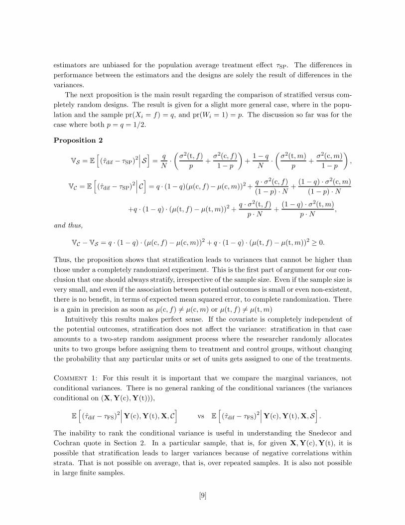
The next proposition is the main result regarding the comparison of stratified versus com-

pletely random designs. The result is given for a slight more general case, where in the popu-

lation and the sample pr(Xi = f) = q, and pr(Wi = 1) = p. The discussion so far was for the

case where both p = q = 1/2.

Proposition 2

VS = E

[

(τdif − τSP)2∣

∣

∣S]

=q

N·

(

σ2(t, f)

p+

σ2(c, f)

1− p

)

+1 − q

N·

(

σ2(t, m)

p+

σ2(c, m)

1 − p

)

,

VC = E

[

(τdif − τSP)2∣

∣

∣C]

= q · (1− q)(µ(c, f)− µ(c, m))2 +q · σ2(c, f)

(1 − p) · N+

(1 − q) · σ2(c, m)

(1 − p) · N

+q · (1− q) · (µ(t, f)− µ(t, m))2 +q · σ2(t, f)

p · N+

(1 − q) · σ2(t, m)

p · N,

and thus,

VC − VS = q · (1 − q) · (µ(c, f)− µ(c, m))2 + q · (1− q) · (µ(t, f)− µ(t, m))2 ≥ 0.

Thus, the proposition shows that stratification leads to variances that cannot be higher than

those under a completely randomized experiment. This is the first part of argument for our con-

clusion that one should always stratify, irrespective of the sample size. Even if the sample size is

very small, and even if the association between potential outcomes is small or even non-existent,

there is no benefit, in terms of expected mean squared error, to complete randomization. There

is a gain in precision as soon as µ(c, f) 6= µ(c, m) or µ(t, f) 6= µ(t, m)

Intuitively this results makes perfect sense. If the covariate is completely independent of

the potential outcomes, stratification does not affect the variance: stratification in that case

amounts to a two-step random assignment process where the researcher randomly allocates

units to two groups before assigning them to treatment and control groups, without changing

the probability that any particular units or set of units gets assigned to one of the treatments.

Comment 1: For this result it is important that we compare the marginal variances, not

conditional variances. There is no general ranking of the conditional variances (the variances

conditional on (X, Y(c), Y(t))),

E

[

(τdif − τFS)2∣

∣

∣Y(c), Y(t), X, C

]

vs E

[

(τdif − τFS)2∣

∣

∣Y(c), Y(t),X,S

]

.

The inability to rank the conditional variance is useful in understanding the Snedecor and

Cochran quote in Section 2. In a particular sample, that is, for given X, Y(c), Y(t), it is

possible that stratification leads to larger variances because of negative correlations within

strata. That is not possible on average, that is, over repeated samples. It is also not possible

in large finite samples.

[9]

There does not appear to be any way to exploit this possibility of negative correlations

within strata, so it is largely of theoretical importance. In practice it means that if the primary

interest is in the most precise estimate of the average effect of the treatment, stratification

dominates complete randomization, even in small samples.

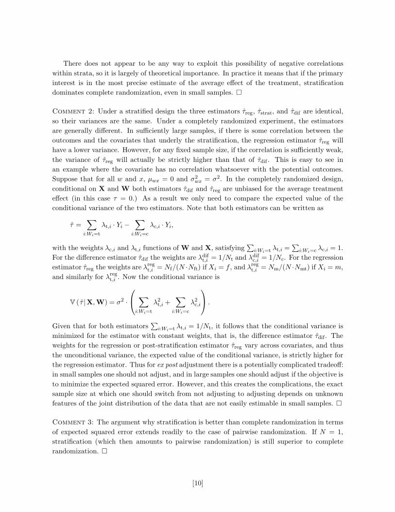
Comment 2: Under a stratified design the three estimators τreg, τstrat, and τdif are identical,

so their variances are the same. Under a completely randomized experiment, the estimators

are generally different. In sufficiently large samples, if there is some correlation between the

outcomes and the covariates that underly the stratification, the regression estimator τreg will

have a lower variance. However, for any fixed sample size, if the correlation is sufficiently weak,

the variance of τreg will actually be strictly higher than that of τdif . This is easy to see in

an example where the covariate has no correlation whatsoever with the potential outcomes.

Suppose that for all w and x, µwx = 0 and σ2wx = σ2. In the completely randomized design,

conditional on X and W both estimators τdif and τreg are unbiased for the average treatment

effect (in this case τ = 0.) As a result we only need to compare the expected value of the

conditional variance of the two estimators. Note that both estimators can be written as

τ =∑

i:Wi=t

λt,i · Yi −∑

i:Wi=c

λc,i · Yi,

with the weights λc,i and λt,i functions of W and X, satisfying∑

i:Wi=t λt,i =∑

i:Wi=c λc,i = 1.

For the difference estimator τdif the weights are λdift,i = 1/Nt and λdif

c,i = 1/Nc. For the regression

estimator τreg the weights are λregt,i = Nf/(N ·Nft) if Xi = f , and λreg

t,i = Nm/(N ·Nmt) if Xi = m,

and similarly for λregt,i . Now the conditional variance is

V ( τ |X, W) = σ2 ·

∑

i:Wi=t

λ2t,i +

∑

i:Wi=c

λ2c,i

.

Given that for both estimators∑

i:Wi=t λt,i = 1/Nt, it follows that the conditional variance is

minimized for the estimator with constant weights, that is, the difference estimator τdif . The

weights for the regression or post-stratification estimator τreg vary across covariates, and thus

the unconditional variance, the expected value of the conditional variance, is strictly higher for

the regression estimator. Thus for ex post adjustment there is a potentially complicated tradeoff:

in small samples one should not adjust, and in large samples one should adjust if the objective is

to minimize the expected squared error. However, and this creates the complications, the exact

sample size at which one should switch from not adjusting to adjusting depends on unknown

features of the joint distribution of the data that are not easily estimable in small samples.

Comment 3: The argument why stratification is better than complete randomization in terms

of expected squared error extends readily to the case of pairwise randomization. If N = 1,

stratification (which then amounts to pairwise randomization) is still superior to complete

randomization.

[10]

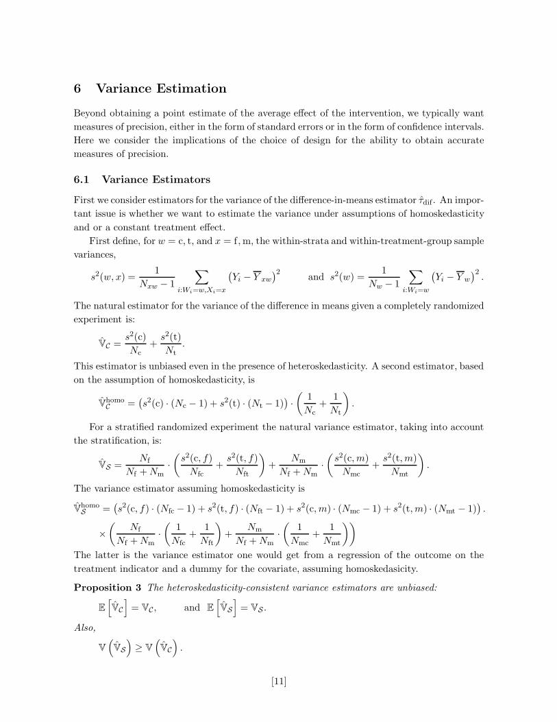
6 Variance Estimation

Beyond obtaining a point estimate of the average effect of the intervention, we typically want

measures of precision, either in the form of standard errors or in the form of confidence intervals.

Here we consider the implications of the choice of design for the ability to obtain accurate

measures of precision.

6.1 Variance Estimators

First we consider estimators for the variance of the difference-in-means estimator τdif . An impor-

tant issue is whether we want to estimate the variance under assumptions of homoskedasticity

and or a constant treatment effect.

First define, for w = c, t, and x = f , m, the within-strata and within-treatment-group sample

variances,

s2(w, x) =1

Nxw − 1

∑

i:Wi=w,Xi=x

(

Yi − Y xw

)2and s2(w) =

1

Nw − 1

∑

i:Wi=w

(

Yi − Y w

)2.

The natural estimator for the variance of the difference in means given a completely randomized

experiment is:

VC =s2(c)

Nc

+s2(t)

Nt

.

This estimator is unbiased even in the presence of heteroskedasticity. A second estimator, based

on the assumption of homoskedasticity, is

VhomoC =

(

s2(c) · (Nc − 1) + s2(t) · (Nt − 1))

·

(

1

Nc

+1

Nt

)

.

For a stratified randomized experiment the natural variance estimator, taking into account

the stratification, is:

VS =Nf

Nf + Nm

·

(

s2(c, f)

Nfc

+s2(t, f)

Nft

)

+Nm

Nf + Nm

·

(

s2(c, m)

Nmc

+s2(t, m)

Nmt

)

.

The variance estimator assuming homoskedasticity is

VhomoS =

(

s2(c, f) · (Nfc − 1) + s2(t, f) · (Nft − 1) + s2(c, m) · (Nmc − 1) + s2(t, m) · (Nmt − 1))

.

×

(

Nf

Nf + Nm

·

(

1

Nfc

+1

Nft

)

+Nm

Nf + Nm

·

(

1

Nmc

+1

Nmt

))

The latter is the variance estimator one would get from a regression of the outcome on the

treatment indicator and a dummy for the covariate, assuming homoskedasicity.

Proposition 3 The heteroskedasticity-consistent variance estimators are unbiased:

E

[

VC

]

= VC, and E

[

VS

]

= VS .

Also,

V

(

VS

)

≥ V

(

VC

)

.

[11]

Both variance estimators are unbiased for the respective variances. Hence, by Proposition 2, the

expectation of VS is less than or equal to the expectation of VC, or E[VS] ≤ E[VC]. Nevertheless,

in a particular sample, with values (Y, W, X), it may well be the case that the realized value

of the completely randomized variance estimator VC(Y, W, X) is less than that of the blocking

variance VS(Y, W, X).

A simple example can show this. Suppose that σ2(c, f) = σ2(c, m) = 0, and that σ2(t, f) =

σ2(t, m) = σ2(t). Then the two variance estimators reduce to

VC =s2(t)

Nt

=Nf

Nf + Nm

·s2(t)

Nft

+Nm

Nf + Nm

·s2(t)

Nmt

,

and

VS =Nf

Nf + Nm

·s2(t, f)

Nft

+Nm

Nf + Nm

·s2(t, m)

Nmt

.

Because σ2(t, f) = σ2(t, m) = σ2(t), it follows that s2(t) is a better estimator for σ2t than

s2(, t, f) and s2(t, m), and therefore VS is a noisier estimator for the same object, in other

words, VC has lower variance than VS , V

(

VC

)

< V

(

VS

)

.

Comment 4: The implication of this is that if the covariate is not associated at all with the

outcomes, than although there is no harm in using the estimator based on stratification in terms

of precision of the point estimator, there is a cost to using the variance estimator corresponding

to the stratification.

Comment 5: It is sometimes suggested to use VC instead of VS even if the design was stratified

instead of completely randomized. What are the issues related that? Using VC instead of VS

leads to an estimator for the variance that is unbiased if the covariate has no explanatory

power at all for the outcomes, but otherwise it leads to an upwardly biased estimator. Thus,

if one intends to use the variance to test the null hypothesis of no effects, the test may have

low power. Ideally in large samples one would want to use the variance estimator taking into

account the stratification, VS . So, another alternative is to take the minimum of the two

variance estimators, V = min(VS , VC). However, this variance estimator is biased downward in

small samples, and so may lead to incorrect size for statistical tests.

6.2 T-statistic Based Tests for Treatment Effects and Degrees of FreedomAdjustments

The comparison between the variance of VC versus the variance of VS is key to understanding

the concerns about stratification and pairwise randomization that have been raised in the

literature. These concerns arise in the context of testing for the presence of treatment effects

based on t-statistics, and in particular in cases where the correlation between the covariates

and the outcomes is small or zero. The t-statistics typically used are

tC =τdif

√

VC

(completely randomized experiment)

[12]

and

tS =τdif

√

VS

(stratified randomized experiment)

Propositions 2 and 3 imply that if the average effect of the treatment differs from zero, then

E[τdif |S] ≥ E[τdif|C], E[VS |S] ≤ E[VC|C], and V

(

VS

)

≥ V

(

VC

)

.

In particular, if the covariates are not associated at all with the outcomes, then

E[τdif |S] = E[τdif|C], E[VS |S] = E[VC|C], and V

(

VS

)

> V

(

VC

)

.

In the last setting it is straightforward to rank the power of the t-statistic based on a completely

randomized experiment and a stratified randomized experiment, at least under normality. The

numerator for both t-statistics is identical, and thus has the same distribution. The denomi-

nators are both independent of the numerator (at least under normality of the outcomes), but

the denominator for VS has a larger variance than the denominator for VC (and in fact this

relation satisfies second order stochastic dominance). Thus the finite sample critical values for

tS would be larger than those for tC . This shows up in standard practice by the degrees of

freedom adjustment. Let cp,C and cp,S be the (unknown, finite sample) critical values for the

two t-tests for the completely randomized and stratified randomized experiment respectively.

Then, cp,C < cp,S. Moreover, under normality and no association between the covariates and

outcomes, we have, for the adjusted critical values,

pr ( |tC | ≥ cp,C| τ) ≥ pr ( |tS | ≥ cp,S| τ) ,

for conventional sizes of the test, p, and all τ 6= 0. This is what the argument against stratifi-

cation is formally based on.

Let me make this more precise in a very specific context. Suppose we have 2N units. We

sample N units from a large population, with covariate values Xi, distributed normally with

mean µX and variance σ2X . We then draw another set of N units, with exactly the same

values for the covariates. We then consider two experimental designs. First, in a completely

randomized design we randomly pick N units out of this set of 2N units to receive the treatment.

Call this design C. Second, we pair the units by the covariate value and randomly assign one unit

from each pair to the treatment. Call this design P . Moreover, suppose that the distribution

of the potential control outcome is

Yi(c)|Xi = N (µ, σ2), and Yi(t) = Yi(c) + τ.

Note that the covariate does not affect the distribution of the potential outcomes at all. The

estimator under both designs is

τdif = Y t − Y c.

Its distribution under the two designs is the same as well:

τdif |C ∼ N (τSP, ) and τdif|P ∼ N

(

τSP,2 · σ2

N

)

.

[13]

The natural estimator for the variance for the estimator given the pairwise randomized exper-

iment is

VP =1

N − 1

N∑

i=1

(τi − τ)2 ∼ σ2 ·X 2(N − 1)

N − 1.

The variance estimator for the completely randomized design, exploiting homoskedasticity, is

VC =(N − 1) · s2(c) + (N − 1) · s2(t)

2N − 2∼ σ2 ·

X 2(2 · N − 2)

2 · N − 2.

Under the normality assumption both variance estimators are independent of τdif . Moreover,

the two variance estimators have the same expectation. The variance of VP is larger than that

of VC

This leads to the t-statistics

tP =τdif

√

VP

, and tC =τdif

√

VC

.

If we wish to test the null hypothesis of τ = 0 against the alternative of τ 6= 0 at level α, we

would reject the null hypothesis if the absolute value of the t-statistic exceeds a critical value

c. For the P design the critical value is

cPα = qt1−α/2(N − 1),

the 1 − α/2 quantile of the t-distribution with N − 1 degrees of freedom. For the completely

randomized design it is

cCα = qt1−α/2(2 · N − 2),

the same quantile for the t-distribution with 2 · N − 2 degrees of freedom.

Proposition 4 For any τ 6= 0, and for any N ≥ 4 the power of the test based on the t-statistic

tC is strictly greater than the power based on the t-statistic tP .

By extension the power for the test based on the completely randomized design is still greater

than the power based on the pairwise randomized experiment if the association between the

covariate and the potential outcomes is weak, at least in small samples. This is the formal

argument against doing a pairwise (or by extension) a stratified randomized experiment if the

covariates are only weakly associated with the potential outcomes.

6.3 The Power of Fisher (Randomization Based) Tests

Here I want to argue that the argument against stratification as opposed to complete random-

ization based on the power of t-tests is is tied intrinsically to the use of a particular test statistic,

rather than reflect on the randomization design directly.

Optimality of tests in the Neyman-Pearson paradigm starts with tests of a sharp null hy-

pothesis against a sharp alternative hypothesis (that is, both the null and alternative hypothesis

[14]

correpsond to a single value of the parameter). In that case we can figure out what the optimal

critical region looks like, and thus what optimal tests are. This sometimes extends to test of a

sharp null hypothesis against a composite alternative hypothesis (where many parameter values

are consistent with the alternative). However, optimality results for the case where the null

hypothesis is a composite hypothesis are generally large sample results, with little known in

finite samples.

What are the implications of this for the current setting? Suppose we are willing to assume

that the distribution of Yi(w) is normal with unknown mean µ(w) (depending on the level of

the treatment) and known common variance σ2. It is key here that the variance is known so

that there are no nuisance parameters and the null hypothesis and alternative hypotheses are

sharp. In that case the optimal test is based on the diference in means Y t −Y c. One can show

that in this case the test based on a stratified design (and by extension a pairwise randomized

design) is more powerful than that based on a completely randomized design, with the power

equal if the covariates are not associated with the outcomes.

Now suppose we relax the assumption of known variances. In that case in large samples the

t-statistic-based test based on a stratified design is still at least as powerful as the test based

on a completely randomized design. However, now it is key that the comparison is in large

samples. In finite samples, the optimality results do not apply and the completely randomized

design leads to a more powerful t-statistic based test than the stratified or paired design if the

covariates are not associated with the potential outcomes.

The t-statistic-based tests are not the only way to go though. Alternative tests can be

attractive because they do not rely on distributional assumptions. In particular Fisher’s exact

p-value approach is an attractive alternative. Suppose we test the null hypothesis of no treat-

ment effect at all, Yi(c) = Yi(t) for all i = 1, . . . , N . Fixing the potential outcomes (taking the

potential outcomes as given), we can look at the distribution of any statistic under the ran-

domization distribution (the distribution generated by assigning different values to W). Let us

use the statistic Y t − Y c. Comparing the power of completely randomized experiments versus

stratified randomized experiments is somewhat tricky because there are only a finite number

of values for the test statistic given fixed values for the potential outcomes. In other words,

the statistic has a discrete distribution. We cannot generally construct tests with exact size

in that case without allowing for randomized tests where for some values for the test statistic

we reject with some probability strictly between zero and one. If we do allow for randomized

tests, then the tests based on stratified randomized experiments have power at least as large

as those based on completely randomized experiments, irrespective of the association between

the potential outcomes and the covariates.

7 Analytic Limitations of Paired Randomized Experiments

Klar and Donner (1997) raise what they call “analytical limitations” of pairwise randomized

experiments. The specific issue that is the biggest concern is the estimation of the variance

conditional on the covariates. Consider first a stratified randomized experiment. As discussed

[15]

earlier, the variance for the average difference estimator in the stratified randomized case is

VS = E

[

(τdif − τSP)2∣

∣

∣S

]

=q

N·

(

σ2(t, f)

p+

σ2(c, f)

1− p

)

+1 − q

N·

(

σ2(t, m)

p+

σ2(c, m)

1 − p

)

,

and the natural unbiased estimator for the variance VS in the two-stratum case is

VS =Nf

Nf + Nm

·

(

s2(c, f)

Nfc

+s2(t, f)

Nft

)

+Nm

Nf + Nm

·

(

s2(c, m)

Nmc

+s2(t, m)

Nmt

)

,

where, for x = f, m, and w = c, t,

s2(w, x) =1

Nxw − 1

∑

i:Wi=w,Xi=x

(

Yi − Y xw

)2.

The difficulty with a pairwise randomized experiment is that we cannot estimate σ2(w, x) with

s2(w, x) because for each value of x and w there is only a single unit, Nxw = 1. What do we do

in practice if we have data from a pairwise randomized experiment? Let i indicate the pairs,

and Wi indicate whether the first member of the pair was assigned to the treatment. Then

define

τi =1

2

2∑

j=1

(Yij(t)− Yij(c)) , so that τFS =1

N

N∑

i=1

τi,

and define

τi = Wi · (Yi1 − Yi2) + (1 − Wi) · (Yi2 − Yi1) .

The estimator for the average treatment effect is

τ =1

N

N∑

i=1

τi,

and the standard variance estimator is

VP =1

N − 1

N∑

i=1

(τi − τ)2 .

Let us investigate the expectation of this variance estimator. Let us for ease of exposition focus

on the case with a total of 4 units, so that Nxw = 1 for x = f, m and w = c, t. The true variance

conditional on the covariates simplifies to

VP =1

2N·

(

σ2(t, f)

1/2+

σ2(c, f)

1/2

)

+1

2N·

(

σ2(t, m)

1/2+

σ2(c, m)

1/2

)

= σ2(t, f)+σ2(c, f)+σ2(t, m)+σ2(c, m).

The expectation of τ is τ (the estimator is obviously unbiased). Then:

E

[

VP

]

= E

[

1

N − 1

N∑

i=1

(τi − τ)2]

[16]

= E

[

1

N − 1

N∑

i=1

((τi − τi) + (τi − τ) + (τ − τ))2

]

= E

[

1

N − 1

N∑

i=1

(τi − τi)2

]

+1

N − 1

N∑

i=1

(τi − τ)2 +N

N − 1E

[

(τ − τ)2]

+2E

[

1

N − 1

N∑

i=1

(τi − τi) (τi − τ) + (τi − τi) (τ − τ) + (τi − τ) (τ − τ)

]

= VP +1

N − 1

N∑

i=1

(τi − τ)2 .

which is larger than VP unless the treatment effect is constant accross pairs. This holds, for

example if the treatment effect is constant across all units, but does not hold in general.

Comment 5: The issue is that within a pair, there is no unbiased estimator for σ2xw. If we

have two treated and two control units in each stratum, then such unbiased estimators do exist,

even if they are noisy. Those unbiased estimators can be used to obtain an unbiased estimator

for τdif . That is ultimately not possible in pairwise randomized experiments, and important

reason to prefer experiments with at least two units of each treatment type in each stratum.

Comment 6: Imai, King and Nall (2009) write that the variance can be estimated consistently,

but this refers to the variance not conditional on the covariates. This variance is larger than

the conditonal one if treatment effects vary by covariates. In stratified randomized experiments

we typically estimate the variance conditional on the strata shares, so the natural extension of

that to paired randomized experiments is to also condition on covariates.

8 Re-Randomization

Another approach that has recently attracted attention especially in the development literature

is re-randomization. The set up is the following. We have N units, and observe for each unit a

vector of covariates Xi. An assignment vector W is drawn, with N/2 units randomly selected

for assignment to the treatment group, and the remainder assigned to the control group. Before

actually implementing the treatment, balance in the covariate distributions is checked. If the

degree of balance is deemed insufficient, the randomization is repeated until an assignment

vector is drawn that leads to sufficient balance.

The key to implementing such a re-randomization scheme, or a restricted randomization

scheme as it is referred to in Hayes and Moulton (2009), is to formally define a subset of

assignment vectors that is deemed well balanced. Then the resulting assignment vector can

be viewed as a random draw from such a subset, and randomization inference is well defined.

In contrast, repeating the randomization until the balance is completely optimized leads to a

subset of two possible assignment vectors, and thus makes an informative analysis based on

randomization inference impossible. Fundamentally such restricted randomization schemes are

[17]

similar to stratified and even completely randomized experiments. There we also rule out some

values for the assignment vector, for example, the assignment vector with all units assigned

to the control group. The difference is that here the set of allowable assignment vectors is

restricted in a more complicated way.

Let us investigate how much we can limit the imbalance if we attempt to balance a number

of covariates at the same time. Suppose we have K covariates, with a distribution centered at

µ and covariance matrix Ω. Suppose now we randomly draw N/2 units for assignment to the

treatment, and assign the remaining N/2 to the control group, consider the difference Xt−Xc.

This difference has approximately a normal distribution:

Xt − Xc ∼ N

(

0,4

N· Ω

)

,

and thus

(N/4)(Xt − Xc)Ω−1(Xt − Xc) ∼ X 2(K).

This implies that, on average, the value of (N/4)(Xt − Xc)Ω−1(Xt − Xc) is equal to K. We

might prefer an assignment vector where the value of this quadratic form is smaller. We may

not be able to find a vector such that Xt − Xc is exactly equal to zero, but we may be able to

get a lot closer. The idea behind restricted randomization is to restrict the set of assignment

vectors to those with relatively low values of a criterion such as (N/4)(Xt −Xc)Ω−1(Xt −Xc).

Generally two approaches have been taken. One is to commit to a pre-specified number of

draws of the assignment vector and take the optimal one according to some criterion. Here it

is important not to search over an unlimited number of draws. In that case one may end up

choosing between the two assignment vectors with the lowest value for the criterion and remove

most randomness in the assignment. The second is to restrict the set of allowable assignment

vectors and redraw until the assignment vector satisfies a particular balance criterion. If one

takes the latter approach, one might want to determine what the say, 0.01 quantile of the

distribution of the criterion is over all assignment vectors, and set the threshold approximately

equal to that quantile.

The specific criterion can take different forms. One could take the quadratic form

(N/4)(Xt − Xc)Ω−1(Xt − Xc).

Alternatively one could use the minimum of the t-statistics,

mink=1:K

∣

∣

∣

∣

∣

Xt.k − Xc,k√

Ωkk4/N

∣

∣

∣

∣

∣

.

Comment 7: The key to restricted randomization experiments is to articulate a priori a clear

criterion for deciding how the eventual assignment will be be determined. This is what allows

the researcher to still use randomization-based inference, e.g., Fisher style p-values.

[18]

9 Weighted Average Treatment Effects

Suppose in addition to the outcome and treatment indicator we observe a covariate Xi, con-

tinuous or discrete. The difference with the previous discussion is that the estimand is now a

function of both potential outcomes and the covariate. To be specific, suppose the target is

τweight,pop =E [λ(Xi) · E [Yi(t)− Yi(c)|Xi]]

E [λ(Xi)],

where λ(x) is a known function of the covariate x. The sample equivalent of this population

estimand is

τweight,sample =

∑Ni=1 λ(Xi) · (Yi(t)− Yi(c))

∑Ni=1 λ(Xi)

.

This apparently simple modification of the target from the unweighted one

τunweighted,sample =1

2

N∑

i=1

(Yi(t)− Yi(c)) ,

creates substantial complications for some analyses. The Fisher exact p-value methods are

not affected. Under the hypothesis of no effects of the treatment whatsoever, the potential

outcomes are still known, and the analysis proceeds exactly as before. However, the properties

of estimators for these estimands under the randomization distribution is more complicated.

To see this, consider the case with just two units, i = 1, 2. Let the weights be λ1 and λ2, so that

the normalized weight for unit 1 is λ = λ1/(λ1 + λ2). Thus, we are interested in the average

effect

τweight,sample = λ ·(

Y1(t)− Y1(c))

+ (1 − λ) ·(

Y2(t)− Y2(c))

.

We randomize the treatment to the first unit, W = W1 = 1 − W2. If W = 1, then we observe

Y1(t) and Y2(c). In that case the natural estimator for any causal effect is Y1(t) − Y2(c). If

W = 0, then we observe Y1(c) and Y2(t), and the natural estimator for any causal effect is

Y2(t)− Y1(c), so that

τ = W ·(

Y1(t)− Y2(c))

+ (1 − W ) ·(

Y2(t)− Y1(c))

.

Suppose the marginal probability of assignment to the treatment is p = pr(W = 1). Then the

expectation of this estimator is

E[τ ] = p ·(

Y1(t)− Y2(c))

+ (1 − p) ·(

Y2(t)− Y1(c))

.

= p · Y1(t)− (1− p) · Y1(c)(1− p) · Y2(t)− p · Y2(c).

If p = 1/2 this is an average causal effect, but it is the unweighted one τunweighted,sample, not the

weighted one τweight,sample.

[19]

How can we estimate τweight,pop without bias? We need to weight the realized outcomes:

τ = 2 ·W ·(

λ · Y1(t)− (1− λ) · Y2(c))

+ 2 · (1 − W ) ·(

(1 − λ) · Y2(t) − λ · Y1(c))

=

λ · Y1(t)− (1 − λ) · Y2(c) if W=1,

(1 − λ) · Y2(t)− λ · Y1(c) if W=0.

If we fix pr(W = 1) = 1/2, the expectation of this estimator is

E[τ ] =(

λ · Y1(t)− (1 − λ) · Y2(c))

+(

(1− λ) · Y2(t)− λ · Y1(c))

.

= λ ·(

Y1(t)− Y1(c))

+ (1− λ) ·(

Y2(t)− p · Y2(c))

= τweight,sample.

Although this estimator is unbiased, it is clearly not an attractive estimator. It would appear

reasonable to insist that an estimator for an average causal effect is a weighted average of

outcomes given treatment minus an average of control outcomes with in both cases the weights

adding up to unity.

We can modify the estimator for the general case by normalizing the weights:

τ =

∑

i:Wi=1 λ(Xi) · Yi∑

i:Wi=1 λ(Xi)−

∑

i:Wi=0 λ(Xi) · Yi∑

i:Wi=0 λ(Xi).

This modification, while clearly reasonable, implies that the estimator is no longer unbiased

under the randomization distribution.

An alternative is to group the units into blocks with similar values of the weights, and then

within the block use unweighted average differences, and weight those by the average within

within the block.

10 Cluster Randomized Experiments and Matched Pair Clus-

ter Randomization

The main substantive argument for randomization at a more aggregate level is concern that the

no-interference assumption that underlies estimates of and inference for causal effects based on

randomization at the unit or individual level is not satisfied. This no-interference assumption

is often more plausible at a more aggregate level. For example, for many educational programs

it is likely that there is interference at the individual level, but less at the class or school level.

Thus, typically cluster randomization is not so a choice as an imperative given the interaction

between units.

Once one commits to a cluster randomized experiment a number of new issues come up.

The main issue has to do with variation in cluster size and the choice of estimand. Suppose we

have a large population of clusters, with cluster sizes for cluster c equal to Mc. Let τ clusterc be

the average effect of the treatment in cluster c. The first important question is whether we are

interested in the unweighted average of the cluster average effects,

τ cluster = E

[

τ clusterc

]

[20]

or the average weighted by cluster size:

τ clusterweighted = E

[

ωc · τclusterc

]

,

where the weights are

ωc =Nc

E[Nc].

In some cases the clusters are all the same size, or at least all of similar size. In that case the

weights are all identical, and the two estimands are the same.

If the focus is on the unweighted average, or if the weights are similar, one can pretty much

do the standard analyses based on unit-level randomization. Define outcomes at the cluster

level, e.g., the average of the unit-level outcomes, averaged over all sampled units in the cluster,

and one can apply all the results from unit-level randomization. The same arguments in favor

of stratification apply directly, and the same reservations about pairwise randomization.

The main issues concern variation in cluster size if the focus is on the weighted average

effect τ clusterweighted.

11 Conclusion

We discuss in this paper the benefits of stratification in randomized experiments. We show that

even in finite samples, irrespective of the (lack of) correlation between covariates and outcomes,

stratification cannot hurt in terms of expected-squared-error. The first qualification is that this

is an ex ante result: conditional on the sample values of the covariates, stratification can make

things worse. The second qualification is that the result requires a random sample from an

infinite population, to avoid the possibility of negative correlations within strata over repeated

samples. Neither of these qualifications appear easy to exploit in practice, and so our conclusion

is that whenever possible, one should stratify, and that there is no systematic tradeoff that one

should assess before deciding to stratify or not.

We a l s o di s cus s t he i m pl i ca t i o ns o f r a ndo m i za t i o n a t t he cl us t er r a t her t ha n t he uni t

level. Clustering induces problems similar to those that arise from being interested in weighted

average treatment effects. The recommended solution is to focus on unweighted averages within

blocks defined by the weights and then average those over the blocks.

[21]

References

Box, G., S. Hunter and W. Hunter, (2005), Statistics for Experimenters: Design, Innovation and

Discovery, Wiley, New Jersey.

Bruhn, M., and D. McKenzie, (2008), “In Pursuit of Balance: Randomization in Practice in

Development Field Experiments,” mimeo, World Bank.

Cox, D., and N. Reid, (2000), The Theory of the Design of Experiments, Chapman and Hall/CRC,

Boca Raton, Florida.

Chase, G., (1968), “On the Efficiency of Matched Pairs in Bernoulli Trials,” Biometrika, Vol 55(2),

365-369.

Diehr, P., D. Martin, T. Koepsell, and A. Cheadle, (1995), “Breaking the Matches in a Paired

t-Test for Coomunity Interventions when the Number of Pairs is Small,” Statistics in Medicine

Vol 14 1491-1504.

Donner, A., (1987), “Statistical Methodology for Paired Cluster Designs,” American Journal of Epi-

demiology, Vol 126(5), 972-979.

Gail, M., S. Mark, R. Carroll, S. Green, and D. Pee, (1996), “On Design Considerations and

Randomization-bsed Inference for Community Intervention Trials,” Statistics in Medicine, Vol 15,

1069-1092.

Imai, K.,, (2008) “Variance Identification and Efficiency Analysis in Randomized Experiments Under

the Matched-Pair Design,” Statistics in Medicine, Vol. 171: 4857-4873.

Imai, K., G. King and C. Nall, (2009) “The Essential Role of Pair Matching in Cluster-Randomized

Experiments, with Application to the Mexican Universal Health Insurance Evaluation,” forthcom-

ing, Statistical Science .

Imai, K., G. King and E. Stuart, (2008) “Misunderstandings among Experimentalists and Obser-

vationalists about Causal Inference,” Journal of the Royal Statistical Society, Series A Vol. 171:

481-502.

Lynn, H., and C. McCulloch, (1992), “When Does it Pay to Break the Matches for Analysis of a

Matched-pair Design,” Biometrics, Vol 48, 397-409.

Martin, D., P. Diehr, E. Perril, and T. Koepsell,, (1993) “The Effect of Matching On the

Power of Randomized Community Intervention Studies,” Statistics in Medicine, Vol. 12: 329-338.

Shipley, M., P. Smith, and M, Dramaix, (1989), “Calculation of Power for Matched Pair Studies

when Randomization is by Group,” International Journal of Epidemiology, Vol 18(2), 457-461.

Snedecor, G., and W. Cochran, (1989), Statistical Methods, Iowa State University Press, Ames,

Iowa.

[22]