Embed Size (px)
Citation preview
EXPERIMENTAL INVESTIGATION ON SHARP CRESTED RECTANGULAR
WEIRS
A THESIS SUBMITTED TO THE GRADUATE SCHOOL OF NATURAL AND APPLIED SCIENCES
OF MIDDLE EAST TECHNICAL UNIVERSITY
BY
H. ÇİĞDEM ŞİŞMAN
IN PARTIAL FULFILLMENT OF THE REQUIREMENTS FOR
THE DEGREE OF MASTER OF SCIENCE IN
CIVIL ENGINEERING
AUGUST 2009

Approval of the thesis:
EXPERIMENTAL INVESTIGATION OF SHARP CRESTED
RECTANGULAR WEIRS
submitted by H. ÇİĞDEM ŞİŞMAN in partial fulfillment of the requirements for the
degree of Master of Science in Civil Engineering Department, Middle East
Technical University by,
Prof. Dr. Canan Özgen _______________
Dean, Graduate School of Natural and Applied Sciences
Prof. Dr. Güney Özcebe _______________
Head of Department, Civil Engineering
Assoc. Prof. Dr. A. Burcu Altan-Sakarya _______________
Supervisor, Civil Engineering Department, METU
Assoc. Prof. Dr. İsmail Aydın _______________
Co-supervisor, Civil Engineering Department, METU
Examining Committee Members:
Prof. Dr. Mustafa Göğüş _______________
Civil Engineering Dept., METU
Assoc. Prof. Dr. A. Burcu Altan-Sakarya _______________
Civil Engineering Dept., METU
Assoc. Prof. Dr. İsmail Aydın _______________
Civil Engineering Dept., METU
Assoc. Prof. Dr. M. Ali Kökpınar _______________
Civil Engineering Dept., METU
Aldonat Köksal (M.Sc, CE) _______________
Company Manager, Hidro Dizayn Eng. Consulting
Construction and Trade Ltd Co.
Date: _______________
iii
I hereby declare that all information in this docum ent has been obtained and presented in accordance with academic rules and ethical conduct. I also declare that, as required by these rules and c onduct, I have fully cited and referenced all material and results that are not original to this work.
Name, Last Name: H. Çiğdem, ŞİŞMAN
Signature :
iv
ABSTRACT
EXPERIMENTAL INVESTIGATION ON SHARP CRESTED
RECTANGULAR WEIRS
Şişman, H. Çiğdem
M.Sc., Department of Civil Engineering
Supervisor : Assoc. Prof. Dr. A. Burcu Altan-Sakarya
Co-Supervisor : Assoc. Prof. Dr. İsmail Aydın
Sharp crested rectangular weirs used for discharge measurement
purposes in open channel hydraulics are investigated experimentally. A series
of experiments were conducted by measuring discharge and head over the
weir for different weir heights for full width weir. It is seen that after a certain
weir height, head and discharge relation does not change. Hence a constant
weir height is determined. For that height; discharge and head over the weir
are measured for variable weir width, starting from the full width weir to slit
weir. Description of the discharge coefficient valid for the full range of weir
widths and an empirical expression involving dimensionless flow variables is
aimed. Experimental data obtained for this purpose and the results of the
regression analysis performed are represented.
Key Words: Flow measurement, Sharp crested weir, Rectangular weir,
Open channel flow
v
ÖZ
DİKDÖRTGEN KESİTLİ KESKİN KENARLI SAVAKLAR ÜZERİNE
DENEYSEL BİR ARAŞTIRMA
Şişman, H. Çiğdem
Yüksek Lisans, İnşaat Mühendisliği Bölümü
Tez Yöneticisi : Doç. Dr. A. Burcu Altan-Sakarya
Ortak Tez Yöneticisi : Doç. Dr. İsmail Aydın
Açık kanal hidroliğinde debi ölçümü amacıyla kullanılan dikdörtgen
kesitli, keskin kenarlı savaklar deneysel olarak incelenmiştir. Öncelikle tam
açıklıkta çeşitli savak yüksekliklerinde deneyler yapılmış olup, bu deneylerde
debi ve savak üstü su yükü ölçülmüştür. Bu deneyler sonucunda belirli bir
savak yüksekliğinden sonra savak üstü su yükü ve debi ilişkisinde bir değişiklik
olmadığı gözlenmiştir. Böylece sabit bir savak yüksekliği belirlenmiştir. Daha
sonra belirlenen sabit savak yüksekliğinde tam açıklıklı savaktan başlayarak,
dar açıklıklı savağa kadar değişken savak genişliği için debi ve savak üstü su
derinliği ölçülmüştür. Böylece tüm savak genişlikleri için geçerli olabilecek bir
debi katsayısının tanımlanması ve boyutsuz akım parametreleri ile
ilişkilendirilerek ampirik bir denklem ile ifade edilmesi amaçlanmıştır. Bu
kapsamda elde edilen deneysel veriler ve uygulanan regresyon analizi
sonuçları sunulmuştur.
Anahtar Kelimeler: Akım ölçümleri, Keskin kenarlı savak, Dikdörtgen
kesitli savak, Açık kanal akımı

vi
To My Family
vii
ACKNOWLEDGMENTS
The author wishes to thank her supervisor Assoc. Prof. Dr. A. Burcu
ALTAN-SAKARYA and co-supervisor Assoc. Prof. Dr. İsmail AYDIN for their
guidance, advice and support throughout the research.
The author would also like express her deepest gratitude to her father
Necmettin Şişman, mother Yasemin Şişman, her sister F. Didem Şişman and
her grandmother Fidan Timurkaynak and also her uncles Hamza Şişman,
Necati Şişman and her cousins A. Filiz Şişman, T. Çağrı Şişman and also Ali
Emre Mutlu and her friends for their love, understanding, trust and support
throughout her whole life.
Finally the author would also like to thank laboratory technicians;
Turgut Ural, Cengiz Tufaner and Hüseyin Gündoğdu for their support and
guidance throughout all experimental works.
viii
TABLE OF CONTENTS
PLAGIARISM………….………………….…………………………………….iii
ABSTRACT……………………………………………………………….…….iv
ÖZ…………………………………………….…………………………………..v
ACKNOWLEDGMENTS………………………………………….…………..vii
TABLE OF CONTENTS……………………………………………..…..…..viii
LIST OF FIGURES…………………………………………….……….…..…..x
LIST OF TABLES………………………………………………………….…..xi
LIST OF SYMBOLS……………………………………………….……..…...xii
CHAPTERS
1. INTRODUCTION ........................................................................................................... 1
1.1. Literature Survey ................................................................................................... 1
1.2. Scope of the Study ............................................................................................... 3
2. THEORETICAL CONSIDERATION ............................................................................ 4
2.1. Definition ................................................................................................................ 4
2.2. Discharge Equation .............................................................................................. 8
2.3. Dimensional Analysis ......................................................................................... 10
3. LITERATURE REVIEW .............................................................................................. 13
3.1. Study of Rehbock (1929) ................................................................................... 14
3.2. Study of Kindsvater and Carter (1957) ............................................................ 15
3.3. Concept of Slit Weir ............................................................................................ 19
4. EXPERIMENTAL STUDIES ....................................................................................... 22
4.1. The Experimental Setup .................................................................................... 22
4.2. Pressure Transducer, Amplifier and Calibration ............................................ 26
4.3. Water Surface Profile ......................................................................................... 30
ix
5. RESULTS AND DISCUSSION .................................................................................. 32
5.1. Introduction .......................................................................................................... 32
5.1.1. Experimental Works for Different Weir Heights ........................................ 33
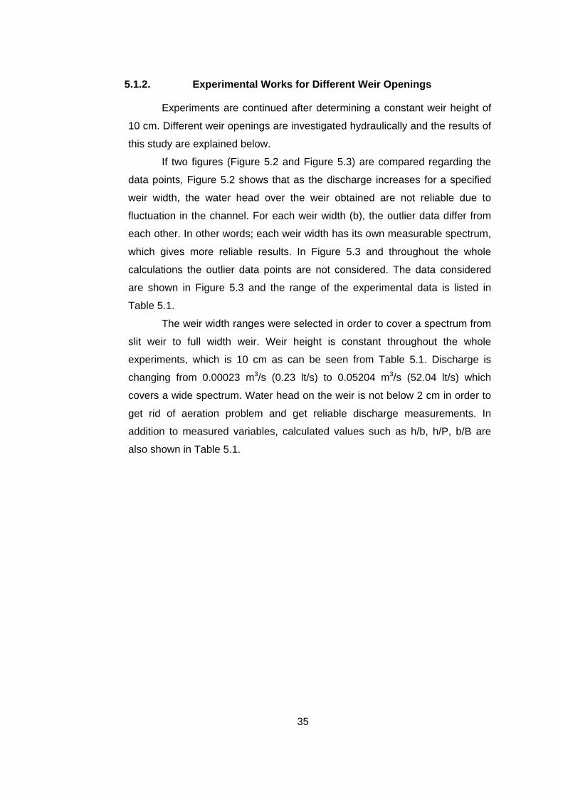
5.1.2. Experimental Works for Different Weir Openings .................................... 35
5.2. Slit Weir ................................................................................................................ 42
5.2.1. Comparison with Kindsvater and Carter (1957) ....................................... 44
5.2.2. Comparison with Aydın et al. (2006) .......................................................... 46
5.3. Contracted Weir .................................................................................................. 49
5.3.1. Comparison with Rehbock (1929) .............................................................. 49
5.3.2. Comparison with Kindsvater and Carter (1957) ....................................... 51
5.4. Present Study ...................................................................................................... 53
6. CONCLUSION ............................................................................................................. 63
REFERENCES ................................................................................................................. 66
x
LIST OF FIGURES
Figure 2.1 The Cross-section Details of Sharp Crested Weirs .............................................. 4
Figure 2.2. The Parameters of Sharp Crested Rectangular Weirs ........................................ 5
Figure 2.3. Types of Sharp Crested Weirs ................................................................................ 6
Figure 2.4 Aerated Nappe ........................................................................................................... 7
Figure 2.5 Non-aerated Nappe .................................................................................................. 7
Figure 2.6 Schematic View of Flow Over Weir ........................................................................ 8
Figure 3.1 The value of Kb with respect to bc/B1 (Bos, 1989) .............................................. 16
Figure 3.2 Graph of Ce versus h1/P1 for values of bc/B1 (Bos, 1989) ........................ 18
Figure 3.4 Graph of Cd versus R with both data points and equation line
(Aydın et al., 2002) .................................................................................................. 20
Figure 3.5 Graph of Cd versus R for different weir openings (b) with both data points
and equation lines (Aydın et al., 2006) ................................................................ 21
Figure 4.1 Front View of Experimental Setup ........................................................................ 22
Figure 4.2 Side View of Experimental Setup.......................................................................... 23
Figure 4.3 Valve and Entrance Structure ............................................................................... 23
Figure 4.4 The Schematic Plan View of Setup ...................................................................... 24
Figure 4.5 The Schematic Profile View of Setup ................................................................... 24
Figure 4.6 Location of Point Gauge on the Channel ............................................................. 25
Figure 4.7 Closer View of Point Gauge ................................................................................... 25
Figure 4.8 Side Plates of Weir for Different Weir Openings ................................................ 26
Figure 4.9 The Amplifier and Computer .................................................................................. 28
Figure 4.10 Amplifier .................................................................................................................... 28
Figure 4.11 Pressure Transducer .............................................................................................. 29
Figure 4.12 Sample of Graph Obtained From Electronic Device .......................................... 29
Figure 4.13 Sections where Water Depths are Measured in Channel ................................. 30
Figure 4.14 Water Surface for Different Discharges ............................................................... 31
Figure 5.1 Relationship Between Discharge (Q) and Head on the Weir (h) for All
Collected Data of Different Weir Heights ............................................................. 34
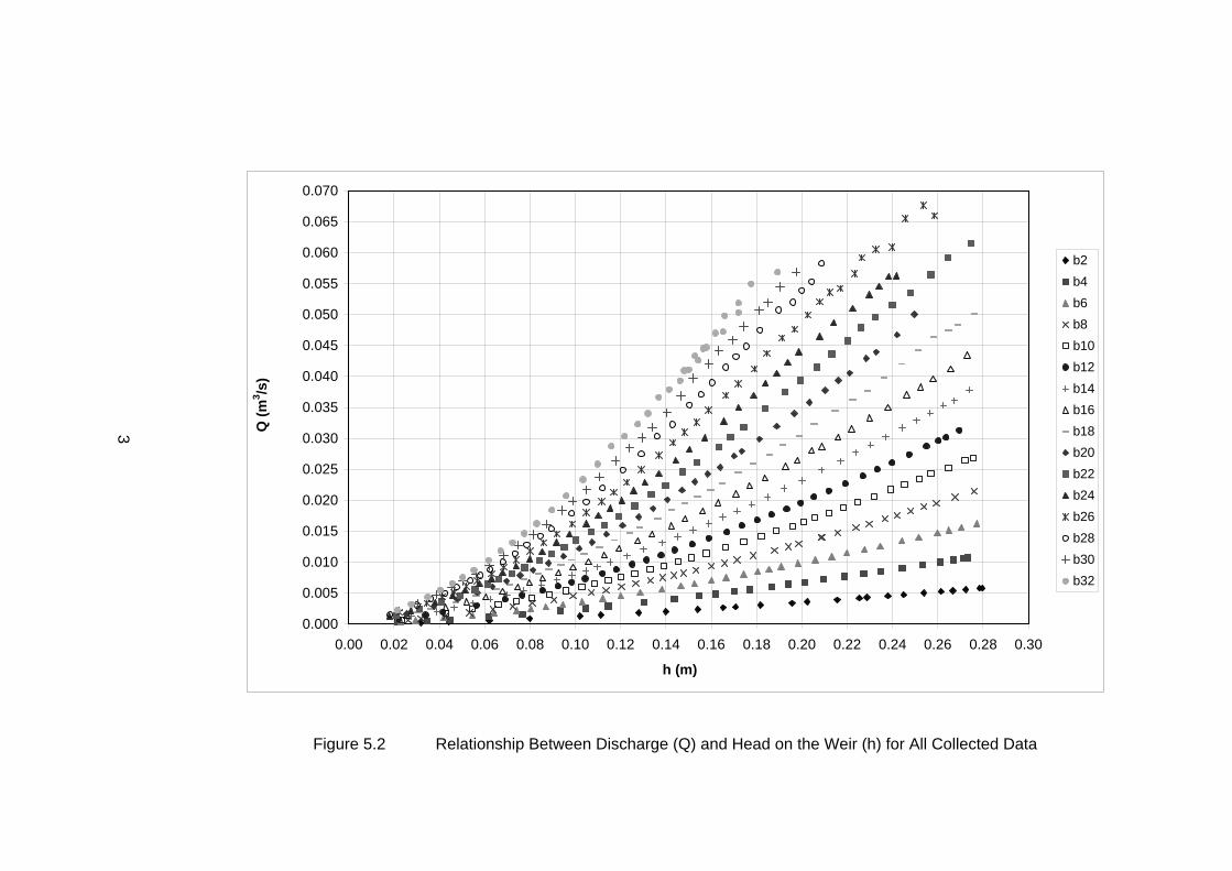
Figure 5.2 Relationship Between Discharge (Q) and Head on the Weir (h) for All
Collected Data ......................................................................................................... 36
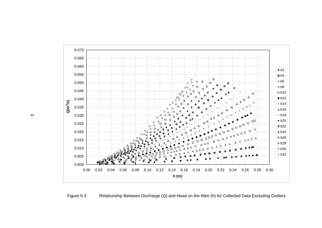
Figure 5.3 Relationship Between Discharge (Q) and Head on the Weir (h) for Collected
Data Excluding Outliers .......................................................................................... 37
Figure 5.4 Cd versus h/b for All Width Openings ................................................................... 40
Figure 5.5 Difference between Slit and Contracted Weir ..................................................... 41
xi
Figure 5.6 Cd versus h/b for Slit Weir ...................................................................................... 42
Figure 5.7 Cd versus Rslit for Slit Weir...................................................................................... 43
Figure 5.8 Cd versus W for Slit Weir ........................................................................................ 44
Figure 5.9 Comparison of Slit Weir Data with Kindsvater and Carter (1957) .................... 45
Figure 5.10 Percent Error with respect to Experimental Discharge ...................................... 46
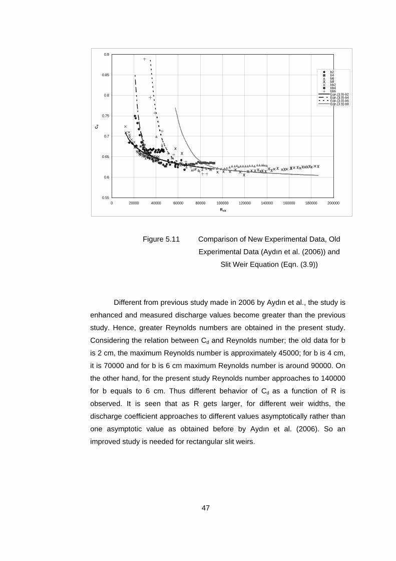
Figure 5.11 Comparison of New Experimental Data, Old Experimental Data
(Aydın et al. (2006)) and Slit Weir Equation (Eqn. (3.9)) ................................... 47
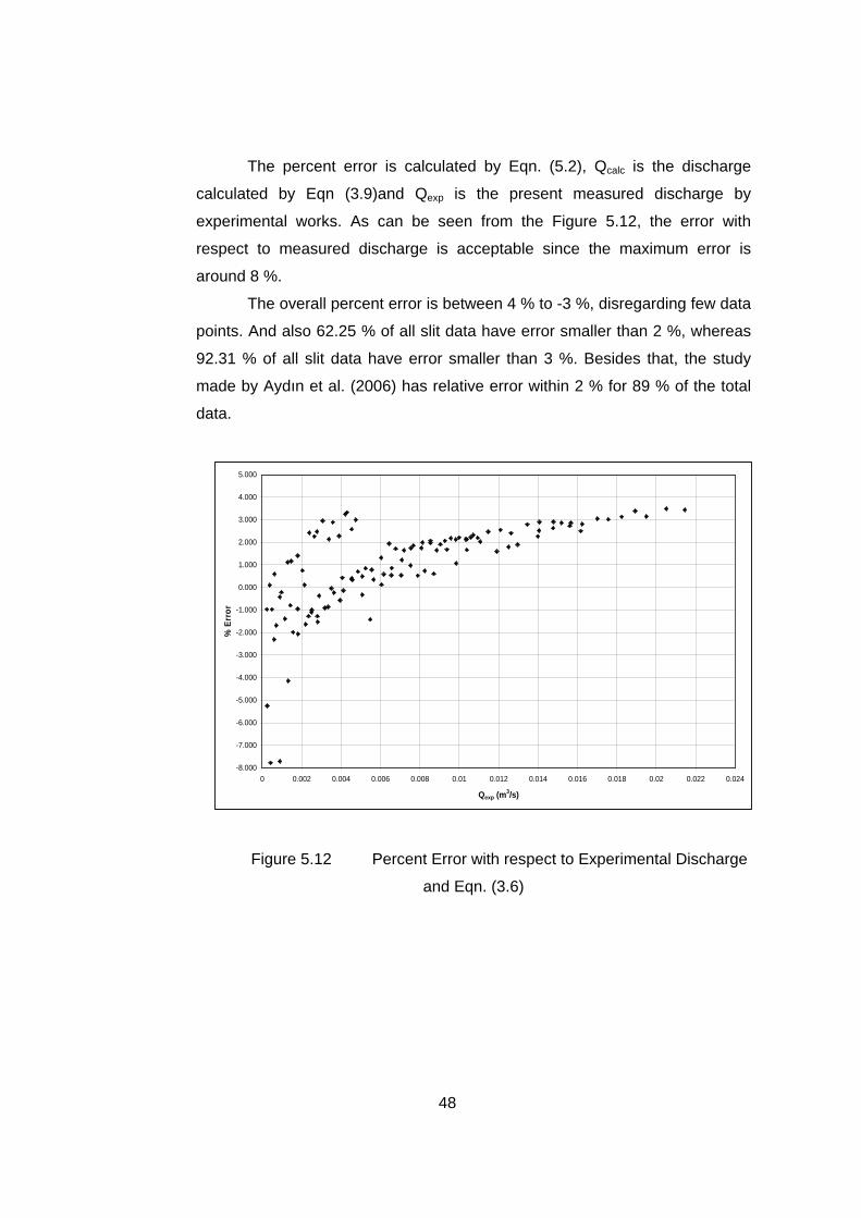
Figure 5.12 Percent Error with respect to Experimental Discharge and Eqn. (3.6) ............ 48
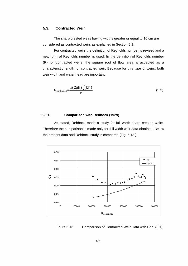
Figure 5.13 Comparison of Contracted Weir Data with Eqn. (3.1) ........................................ 49
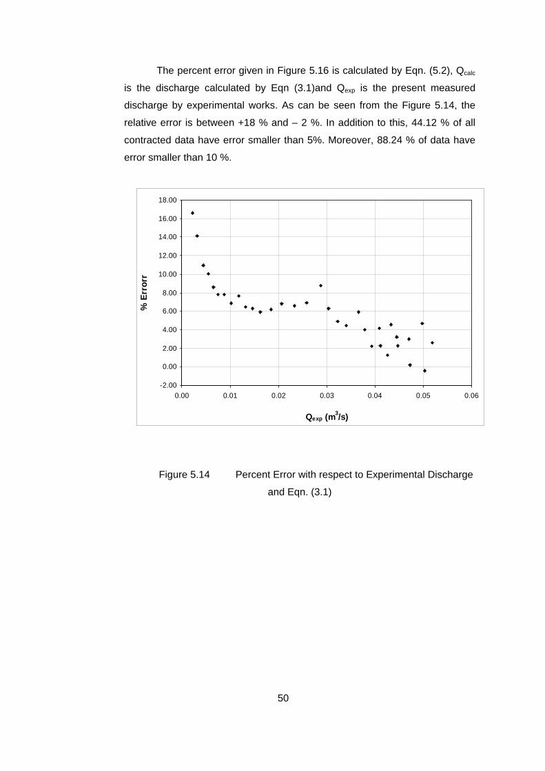
Figure 5.14 Percent Error with respect to Experimental Discharge and Eqn. (3.1) ............ 50
Figure 5.15 Comparison of Contracted Weir Data with Eqn. (3.3) ........................................ 51
Figure 5.16 Percent Error with respect to Experimental Discharge and Eqn. (3.3) ............ 52
Figure 5.17 c1 versus b/B ............................................................................................................ 54
Figure 5.18 c2 versus b/B ............................................................................................................ 55
Figure 5.19 c3 versus b/B ............................................................................................................ 55
Figure 5.20 Q and h Relation for Comparison of Measured with Eqn. (5.4) ....................... 57
Figure 5.21 Cd and h/b Relation for Comparison of Measured Data with Those
Calculated by Eqn. (5.4) ......................................................................................... 59
Figure 5.22 Cd and Rcontracted Relation for Comparison of Measured Data with Those
Calculated by Eqn. (5.4) ......................................................................................... 60
Figure 5.23 Cd and W Relation for Comparison of Measured Data with Those Calculated
by Eqn. (5.4) ............................................................................................................. 61
Figure 5.24 Percent Error with respect to Experimental Discharge and Eqn. (5.4) ............ 62

xii
LIST OF TABLES
Table 3.1 Limitations of Rehbock’s Experimental Study ..................................................... 14
Table 3.2 Effective Discharge Coefficient as a Function of bc/B1 and h1/P1..................... 17
Table 3.3 Limitations of a fully contracted sharp crested rectangular weir (Bos, 1989) . 19
Table 4.1 Water Depth for Different Discharge Conditions ................................................ 31
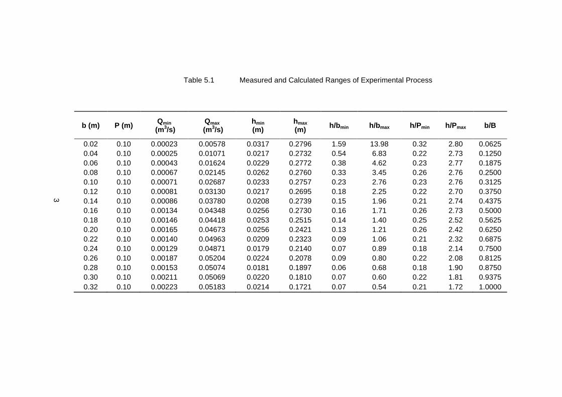
Table 5.1 Measured and Calculated Ranges of Experimental Process ........................... 38
Table 5.2 Values of Constants as a Result of Regression Analysis ................................. 54

xiii
LIST OF SYMBOLS
AT : Area of Tank
b : Width of the Weir
bc : Width of the Weir (Kindsvater and Carter (1957))
be : Effective Width of the Weir
B : Width of the Channel
B1 : Width of the Channel (Kindsvater and Carter (1957))
C : Calibration Constant
Cd : Discharge Coefficient
Ce : Effective Discharge Coefficient
g : Gravitational Acceleration
γ : Specific Weight of Fluid
h : Head on the Weir
he : Effective Head on the Weir
hT : Water Height in the Tank
h1 : Head on the Weir (Kindsvater and Carter (1957))
H1 : Total Head at Section 1
H2 : Total Head at Section 1
Kb : Quantity Represents the Effect of Viscosity and Surface Tension
Kh : Quantity Represents the Effect of Viscosity and Surface Tension
l : Characteristic Length
µ : Dynamic Viscosity of Fluid
ν : Kinematic Viscosity of Fluid
xiv
P : Weir Height
Ps1: Pressure at Section 1
Ps2: Pressure at Section 2
P1 : Weir Height (Kindsvater and Carter (1957))
Q : Discharge
R : Reynolds Number
ρ : Density of Fluid
σ : Surface Tension
t : Time
u : Average Velocity
uT : Average Velocity in the Tank
u1 : Average Velocity at Section 1
u2 : Average Velocity at Section 2
V : Characteristic Velocity
W : Weber Number
z1 : Elevation at Section 1
z2 : Elevation at Section 2
1
1. CHAPTER 1
INTRODUCTION
Measurement of discharge in open channels is one of the main
concerns in hydraulic engineering. Sharp crested weirs (also called thin-plate
weirs or notches) are used to measure discharge in open channels by using
the principle of rapidly varied flow. They are extensively used in laboratories,
industries, irrigation practice and also used as dam instrumentation device.
Thus accurate flow measurement is very important.
In recent years, many researchers made studies in order to measure
discharge over the weirs exactly. Some of these studies are experimental
whereas some of them are theoretical. These studies may be categorized
upon the type of the weir and limitations of the research. Section 1.1 gives
brief information about recent studies.
Wide range of data is studied in present study experimentally. Initially,
experiments are conducted for different weir heights in order to determine a
constant weir height where head and discharge relation does not change.
Then different weir openings are investigated from slit weir to full width weir. In
Section 1.2 summary and scope of the present study are mentioned.
1.1. Literature Survey
For many years sharp crested rectangular weirs have been
investigated by many researchers. The common objective of these studies is
to investigate the flow behaviour of weirs and to obtain a discharge coefficient
which describes the real behaviour. Some of them are explained below briefly.
In 1929 Rehbock performed experiments with small discharges and
concluded with a discharge coefficient equation of full width sharp crested weir
(Franzini and Finnemore, 1997). Rehbock showed that discharge coefficient
2
depends on water height on the weir (h) and the ratio of the water head to the
weir height (h/P). The details of this study are explained in Section 3.1 below.
Kindsvater and Carter made an extensive empirical investigation in
1957 (Bos, 1989). They introduced a number of discharge coefficient
equations as a function of the water head on the weir over the weir height
(h/P) and weir width over the channel width (b/B). This investigation is given in
Section 3.2, since it is used to compare the present study.
Kandaswamy and Rouse (1957) obtained discharge coefficients on
the basis of experimental results. The results of their study based on three
different ranges, such that h/P≤5, 5<h/P<15 and h/P≥15.
Ramamurthy et al. (1987) conducted experiments with a weir range of
0<h/P<10 and sill range of 10≤P/h≤∞. Using momentum principle and
experimental results, a relationship between discharge coefficient and
parameter h/P (or P/h for sills) is obtained. And also velocity and pressure
distributions in the region of nappe and on the weir face are investigated.
Swamee (1988) proposed a generalized weir equation for sharp-
crested, narrow-crested, broad-crested and long-crested weirs by combining
the equations obtained from previous works. The discharge coefficient
equation, suggested by Swamee, depends on geometric characteristics of the
weir, such as weir height, head on the weir and crest width.
Aydın et al. (2002) introduced the term slit weir which is suitable for
measuring small discharges. At the end of their study they found a discharge
coefficient equation in terms of Reynolds number. And in 2006 they improved
the term slit weir and concluded with a discharge equation depending on
Reynolds number and dimensionless number h/b. These two issues are drawn
out below, in Section 3.3.
Ramamurthy et al. (2007) made an experimental investigation on
“multislit weir” in order to extend the slit weir concept and measure not only
very low discharge rates but also very high discharge rates accurately. They
used three different multislit weir units (n=3,7 and 15) and weir opening of 5
mm. And they concluded that discharge coefficient depends on Reynolds
number. But for large values of Reynolds number “inertial forces are high and
viscous forces are negligible” which means that Cd does not depend on
Reynolds number. They also showed that multislit weir can be used to
measure wide range of discharge rates.
3
1.2. Scope of the Study
In the present study, rectangular sharp crested weirs are investigated
experimentally. Several experiments have been conducted with rectangular
sharp crested weirs in laboratory. First of all, water surface profile investigation
is made in order to determine the appropriate location for water head readings.
Then, different weir heights of full width sharp crested rectangular weirs are
investigated. Thus a constant weir height that is free from bottom boundary
effect, is determined. Finally, the experimental study of different weir openings
is made by keeping the weir height constant. Types of sharp crested
rectangular weirs which are investigated vary from slit weir to full width weir.
In Chapter 2, the theoretical aspect of the subject is clarified. In
Chapter 3 the earlier studies are presented and the ones that are used to
compare with the present study are explained in detail. In Chapter 4, the
present experimental setup and procedure are explained. The results of
experimental study and comparison with previous studies are given in Chapter
5. Finally, in Chapter 6 conclusions of the deliberation are drawn out.
4
2. CHAPTER 2
THEORETICAL CONSIDERATION
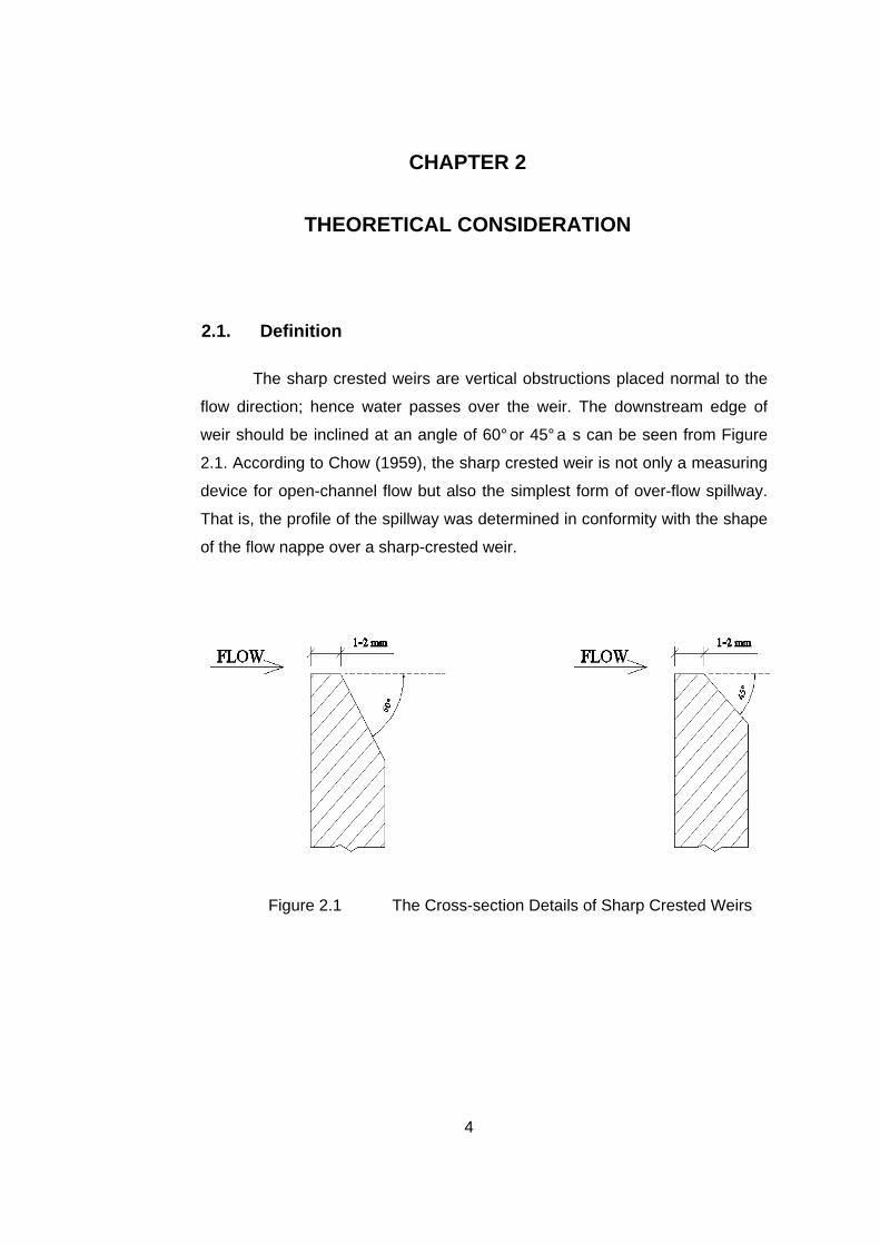
2.1. Definition
The sharp crested weirs are vertical obstructions placed normal to the
flow direction; hence water passes over the weir. The downstream edge of
weir should be inclined at an angle of 60° or 45° a s can be seen from Figure
2.1. According to Chow (1959), the sharp crested weir is not only a measuring
device for open-channel flow but also the simplest form of over-flow spillway.
That is, the profile of the spillway was determined in conformity with the shape
of the flow nappe over a sharp-crested weir.
Figure 2.1 The Cross-section Details of Sharp Crested Weirs
5
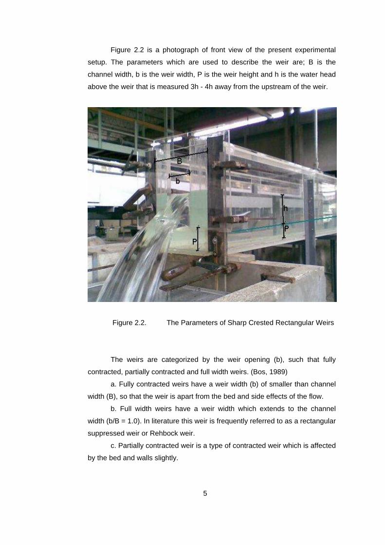
Figure 2.2 is a photograph of front view of the present experimental
setup. The parameters which are used to describe the weir are; B is the
channel width, b is the weir width, P is the weir height and h is the water head
above the weir that is measured 3h - 4h away from the upstream of the weir.
Figure 2.2. The Parameters of Sharp Crested Rectangular Weirs
The weirs are categorized by the weir opening (b), such that fully
contracted, partially contracted and full width weirs. (Bos, 1989)
a. Fully contracted weirs have a weir width (b) of smaller than channel
width (B), so that the weir is apart from the bed and side effects of the flow.
b. Full width weirs have a weir width which extends to the channel
width (b/B = 1.0). In literature this weir is frequently referred to as a rectangular
suppressed weir or Rehbock weir.
c. Partially contracted weir is a type of contracted weir which is affected
by the bed and walls slightly.
6
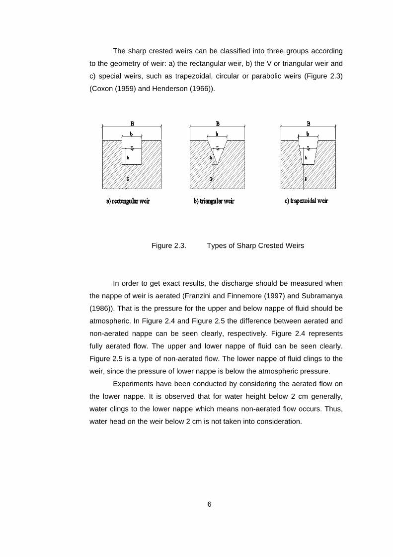
The sharp crested weirs can be classified into three groups according
to the geometry of weir: a) the rectangular weir, b) the V or triangular weir and
c) special weirs, such as trapezoidal, circular or parabolic weirs (Figure 2.3)
(Coxon (1959) and Henderson (1966)).
Figure 2.3. Types of Sharp Crested Weirs
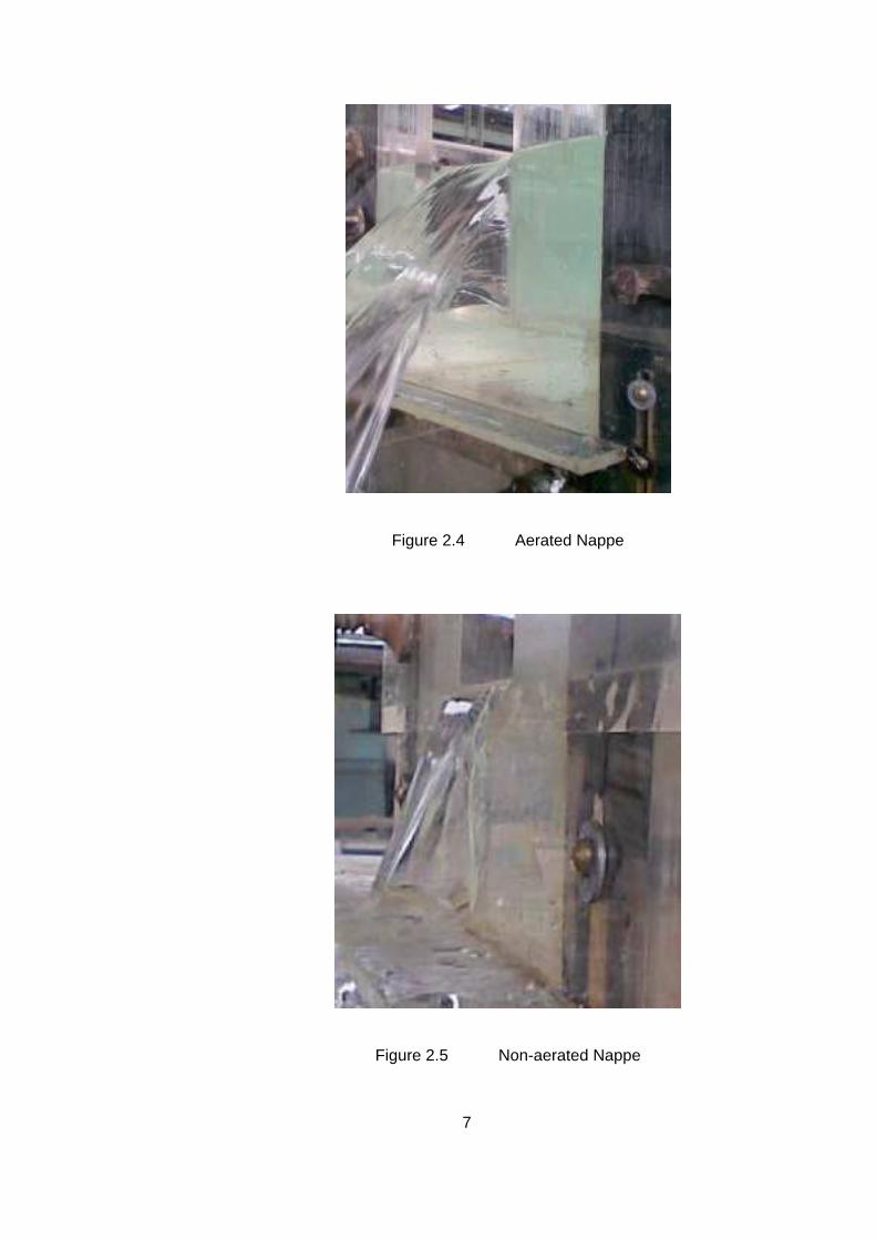
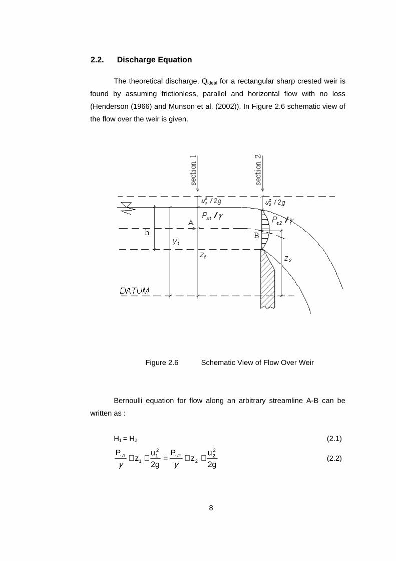
In order to get exact results, the discharge should be measured when
the nappe of weir is aerated (Franzini and Finnemore (1997) and Subramanya
(1986)). That is the pressure for the upper and below nappe of fluid should be
atmospheric. In Figure 2.4 and Figure 2.5 the difference between aerated and
non-aerated nappe can be seen clearly, respectively. Figure 2.4 represents
fully aerated flow. The upper and lower nappe of fluid can be seen clearly.
Figure 2.5 is a type of non-aerated flow. The lower nappe of fluid clings to the
weir, since the pressure of lower nappe is below the atmospheric pressure.
Experiments have been conducted by considering the aerated flow on
the lower nappe. It is observed that for water height below 2 cm generally,
water clings to the lower nappe which means non-aerated flow occurs. Thus,
water head on the weir below 2 cm is not taken into consideration.
7
Figure 2.4 Aerated Nappe
Figure 2.5 Non-aerated Nappe
8
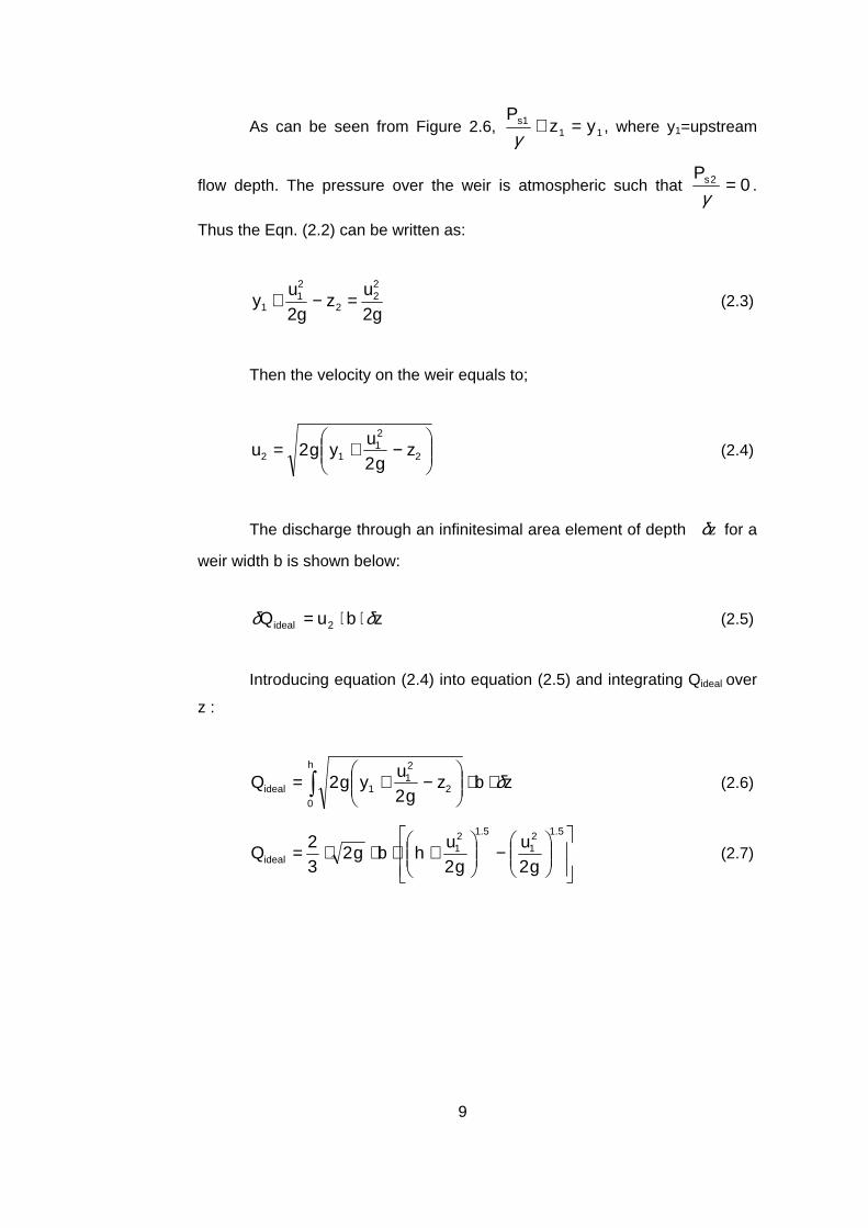
2.2. Discharge Equation
The theoretical discharge, Qideal for a rectangular sharp crested weir is
found by assuming frictionless, parallel and horizontal flow with no loss
(Henderson (1966) and Munson et al. (2002)). In Figure 2.6 schematic view of
the flow over the weir is given.
Figure 2.6 Schematic View of Flow Over Weir
Bernoulli equation for flow along an arbitrary streamline A-B can be
written as :
H1 = H2 (2.1)
g
uz
P
g
uz
P ss
22
22
22
21
11 ++=++
γγ (2.2)
9
As can be seen from Figure 2.6, 11s1 yz
P=+
γ, where y1=upstream
flow depth. The pressure over the weir is atmospheric such that 02 =γsP
.
Thus the Eqn. (2.2) can be written as:
2gu
z2gu
y22
2
21
1 =−+ (2.3)
Then the velocity on the weir equals to;
−+= 2
21
12 zg2
uyg2u (2.4)
The discharge through an infinitesimal area element of depth zδ for a
weir width b is shown below:
zbuQ 2ideal δδ ⋅⋅= (2.5)
Introducing equation (2.4) into equation (2.5) and integrating Qideal over
z :
∫ ⋅⋅
−+=
h
02
21
1ideal zbzg2
uyg2Q δ (2.6)
−
+⋅⋅⋅=
5.121
5.121
ideal g2u
g2u
hbg232
Q (2.7)
10
The velocity head at section 1 can be assumed negligible. Hence the
equation of theoretical discharge is expressed as :
2/3ideal bhg2
32
Q = (2.8)
But the actual discharge, which depends on many parameters such as
viscosity, surface tension, geometry of weir and so on, is given below.
2/3dactual bhg2
32
CQ = (2.9)
where Cd=discharge coefficient which accounts for the accuracy of
discharge.
2.3. Dimensional Analysis
The discharge passing over the weir is a function of several
parameters (Figure 2.2), which is mathematically expressed by equation
(2.10).
( )σµρ ,,,,,,, gPBbhfQ 1= (2.10)
where h=head over the weir crest
b=weir width
B=channel width
P=height of weir
ρ =density of fluid
µ =dynamic viscosity of fluid
g=gravitational acceleration
σ =surface tension
11
A dimensional analysis is performed to find a relation between the
discharge coefficient and other parameters stated above. Below a
mathematical expression of this relation is given.
=Ph
,Bb
,bh
,W,RfbhgQ
22/32/1 (2.11)
Since the discharge equation can be expressed such that :
2/3d bhg2
32
CQ = (2.12)
Thus the discharge coefficient equals to :
( ) 2/32/1dbhg232
QC = (2.13)
Finally Eqn. (2.11) can be written as Eqn. (2.14). As can be seen, the
discharge coefficient depends on Reynolds number, Weber number and
geometry of weir and channel.
=Ph
,Bb
,bh
,W,RfC 3d (2.14)
where R=Reynolds number
W=Weber number
12
The general definition of Reynolds number and Weber number are
given in Eqn. (2.15) and Eqn. (2.16) respectively In most fluid mechanics
problems, by means of dimensionless numbers, there will be a characteristic
velocity, length and fluid property such as viscosity and density.. For special
conditions, different characteristic length and velocity definitions can be used.
In this study two different Reynolds number definitions are used and details of
this topic is explained in following sections.
υlVR = (2.15)
σρ
σρ ghb2V
W2
== l (2.16)
13
3. CHAPTER 3
LITERATURE REVIEW
For sharp crested rectangular weirs, measuring discharge accurately is
very important. And since the discharge, which is needed to be found,
depends on many parameters such as viscosity, surface tension and
geometry, it is difficult to calculate the exact value of discharge. So many
researches have been made to find an accurate equation of discharge
coefficient. Some of these researches are explained in Section 1.1.
In this chapter details of some of the previous studies, which are further
used in order to compare the present study, are explained. The conclusions,
limitations of the studies and suggested equations are drawn out. The details
of studies, which are considered in this section, are listed below;
• Rehbock (1929)
• Kindsvater and Carter (1957)
• Aydın et al. (2002)
• Aydın et al (2006).
The comparison of previous works with the present study and results of
the comparison are explained in Chapter 5 Results and Discussion. The
graphs are illustrated in order to make the subject clearer. And also in Chapter
5, the percent difference between present study and previous studies study is
given.
14
3.1. Study of Rehbock (1929)
Rehbock (1929) made experiments of full width sharp crested weirs.
And at the end of experimental works he concluded with a discharge
coefficient equation which depends on water head on the weir (h) and weir
height (P). The empirical equations of discharge and discharge coefficient are
given in equations (3.1) and (3.2), respectively.
23232 /
d bhgCQ = (3.1)
hPh
..Cd 10001
0806110 ++= (3.2)
Rehbock’s formula has been found to be accurate within 0.5% for
values of P from 0.33 to 3.3 ft (0.1 to 1.0 m) and for values of h from 0.08 to 2
ft (0.025 to 0.60 m) with the ratio h/P not greater than 1.0 (Franzini &
Finnemore, 1997). The limitations of Rehbock’s study are also listed in Table
3.1 below.
Table 3.1 Limitations of Rehbock’s Experimental Study
0.10 m ≤ P < 1.00 m
0.025 m ≤ h < 0.60 m
h / P < 1.00
15
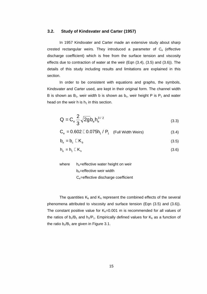
3.2. Study of Kindsvater and Carter (1957)
In 1957 Kindsvater and Carter made an extensive study about sharp
crested rectangular weirs. They introduced a parameter of Ce (effective
discharge coefficient) which is free from the surface tension and viscosity
effects due to contraction of water at the weir (Eqn (3.4), (3.5) and (3.6)). The
details of this study including results and limitations are explained in this
section.
In order to be consistent with equations and graphs, the symbols,
Kindsvater and Carter used, are kept in their original form. The channel width
B is shown as B1, weir width b is shown as bc, weir height P is P1 and water
head on the weir h is h1 in this section.
23232 /
eee hbgCQ = (3.3)
1107506020 P/h..Ce += (Full Width Weirs) (3.4)
bce Kbb += (3.5)
he Khh += 1 (3.6)
where he=effective water height on weir
be=effective weir width
Ce=effective discharge coefficient
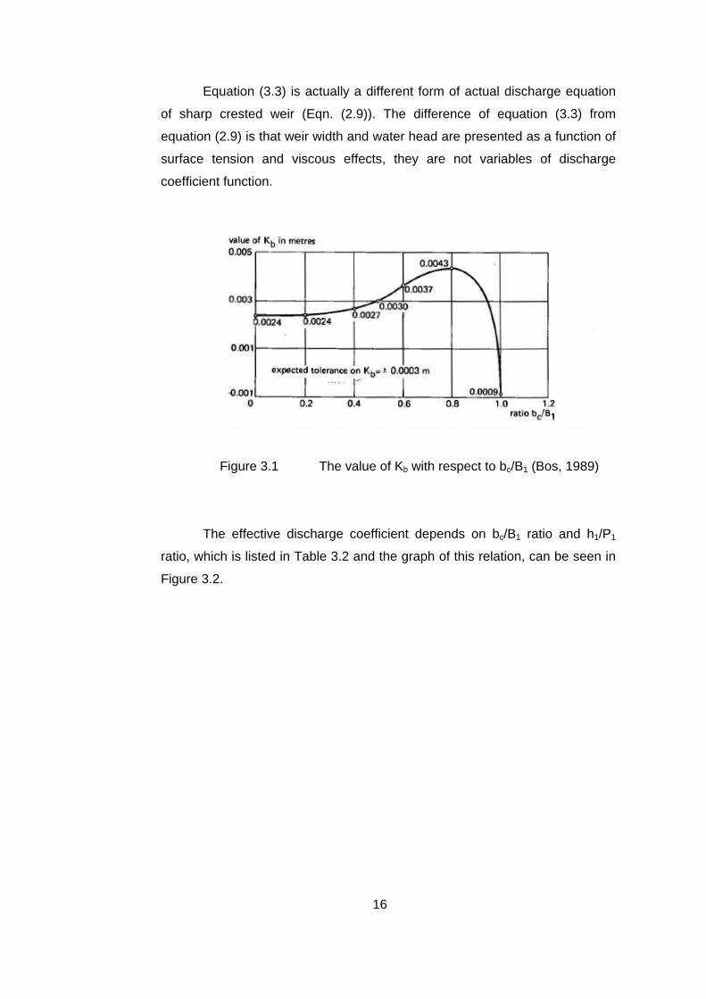
The quantities Kb and Kh represent the combined effects of the several
phenomena attributed to viscosity and surface tension (Eqn (3.5) and (3.6)).
The constant positive value for Kh=0.001 m is recommended for all values of
the ratios of bc/B1 and h1/P1. Empirically defined values for Kb as a function of
the ratio bc/B1 are given in Figure 3.1.
16
Equation (3.3) is actually a different form of actual discharge equation
of sharp crested weir (Eqn. (2.9)). The difference of equation (3.3) from
equation (2.9) is that weir width and water head are presented as a function of
surface tension and viscous effects, they are not variables of discharge
coefficient function.
Figure 3.1 The value of Kb with respect to bc/B1 (Bos, 1989)
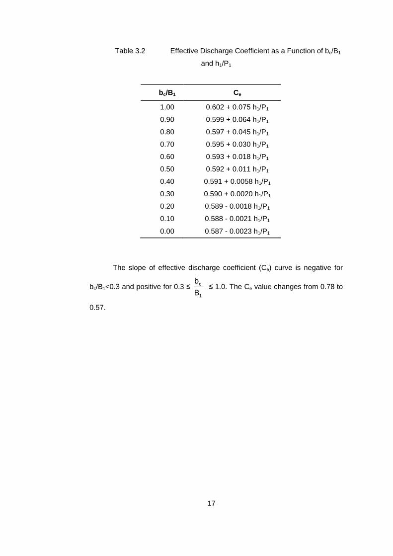
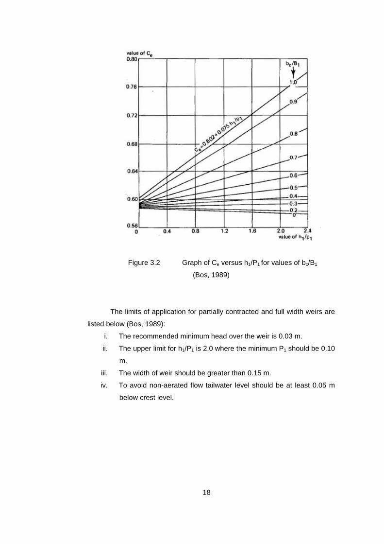
The effective discharge coefficient depends on bc/B1 ratio and h1/P1
ratio, which is listed in Table 3.2 and the graph of this relation, can be seen in
Figure 3.2.
17
Table 3.2 Effective Discharge Coefficient as a Function of bc/B1
and h1/P1
bc/B1 Ce
1.00 0.602 + 0.075 h1/P1
0.90 0.599 + 0.064 h1/P1
0.80 0.597 + 0.045 h1/P1
0.70 0.595 + 0.030 h1/P1
0.60 0.593 + 0.018 h1/P1
0.50 0.592 + 0.011 h1/P1
0.40 0.591 + 0.0058 h1/P1
0.30 0.590 + 0.0020 h1/P1
0.20 0.589 - 0.0018 h1/P1
0.10 0.588 - 0.0021 h1/P1
0.00 0.587 - 0.0023 h1/P1
The slope of effective discharge coefficient (Ce) curve is negative for
bc/B1<0.3 and positive for 0.3 ≤ 1
c
B
b ≤ 1.0. The Ce value changes from 0.78 to
0.57.
18
Figure 3.2 Graph of Ce versus h1/P1 for values of bc/B1
(Bos, 1989)
The limits of application for partially contracted and full width weirs are
listed below (Bos, 1989):
i. The recommended minimum head over the weir is 0.03 m.
ii. The upper limit for h1/P1 is 2.0 where the minimum P1 should be 0.10
m.
iii. The width of weir should be greater than 0.15 m.
iv. To avoid non-aerated flow tailwater level should be at least 0.05 m
below crest level.
19
And finally the limitations of fully contracted sharp crested weir are
given in Table 3.3.
Table 3.3 Limitations of a fully contracted sharp crested
rectangular weir (Bos, 1989)
B1-bc ≥ 4h1
h1/P1 ≤ 0.5
h1/bc ≤ 0.5
0.07 m ≤ h1 < 0.60 m
bc ≥ 0.30 m
P1 ≥ 0.30 m
3.3. Concept of Slit Weir
In 2002 Aydın et al. introduced the term “slit weir”. This type of weir is a
narrow rectangular sharp crested weir, efficient to measure small discharges
accurately. At the end of the study, they found an empirical equation, which
depends on Reynolds number (Eqn (3.7)). The ranges of data are listed
below:
• b (m) = 0.005, 0.01, 0.015, 0.02, 0.03, 0.04, 0.05, 0.075
• P (m) = 0.04, 0.08, 0.16
• Q (m3/s) = 0.00003 – 0.005
As a result the discharge coefficient is:
50354115620 .d R..C += (3.7)
where
υhQR = (3.8)
20
The root mean square error in predicting discharge using Eqn. (3.7) is
calculated as 0.0096 by Aydın et. al (2002). And also 80 % of the data is within
the ±1 % of the value predicted by Eqn. (3.7).
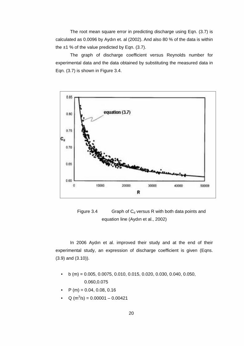
The graph of discharge coefficient versus Reynolds number for
experimental data and the data obtained by substituting the measured data in
Eqn. (3.7) is shown in Figure 3.4.
Figure 3.4 Graph of Cd versus R with both data points and
equation line (Aydın et al., 2002)
In 2006 Aydın et al. improved their study and at the end of their
experimental study, an expression of discharge coefficient is given (Eqns.
(3.9) and (3.10)).
• b (m) = 0.005, 0.0075, 0.010, 0.015, 0.020, 0.030, 0.040, 0.050,
0.060,0.075
• P (m) = 0.04, 0.08, 0.16
• Q (m3/s) = 0.00001 – 0.00421
21
As a result the discharge coefficient is
( )[ ]{ }450
1221105620
.d Rb/hexp
.C−
−−+= (3.9)
For h/b > 2 :
450105620 .d R.C += (3.10)
where
υb)gh(R 2= (3.11)
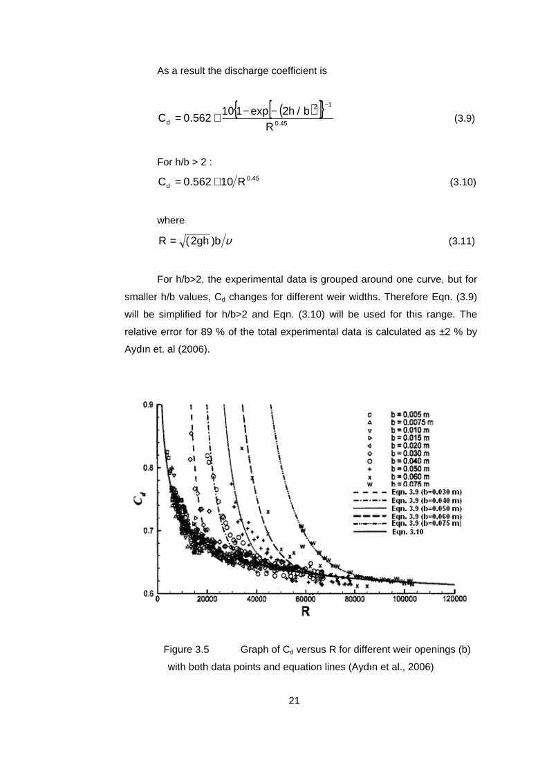
For h/b>2, the experimental data is grouped around one curve, but for
smaller h/b values, Cd changes for different weir widths. Therefore Eqn. (3.9)
will be simplified for h/b>2 and Eqn. (3.10) will be used for this range. The
relative error for 89 % of the total experimental data is calculated as ±2 % by
Aydın et. al (2006).
Figure 3.5 Graph of Cd versus R for different weir openings (b)
with both data points and equation lines (Aydın et al., 2006)
22
4. CHAPTER 4
EXPERIMENTAL STUDIES
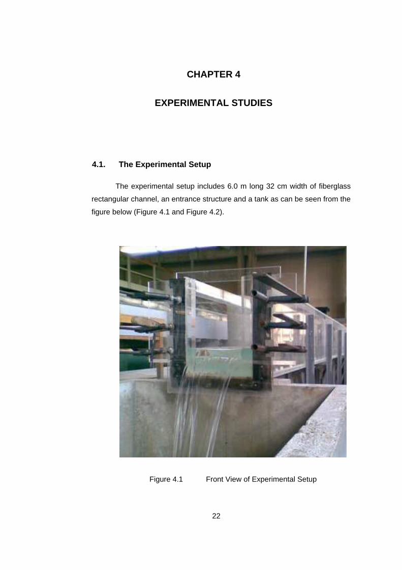
4.1. The Experimental Setup
The experimental setup includes 6.0 m long 32 cm width of fiberglass
rectangular channel, an entrance structure and a tank as can be seen from the
figure below (Figure 4.1 and Figure 4.2).
Figure 4.1 Front View of Experimental Setup
23
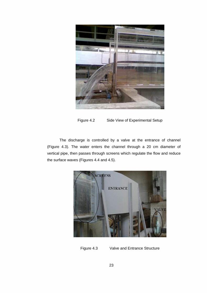
Figure 4.2 Side View of Experimental Setup
The discharge is controlled by a valve at the entrance of channel
(Figure 4.3). The water enters the channel through a 20 cm diameter of
vertical pipe, then passes through screens which regulate the flow and reduce
the surface waves (Figures 4.4 and 4.5).
Figure 4.3 Valve and Entrance Structure
24
WEIRFLOW
ENTRANCE CHANNEL TANK
dimension are in cm.
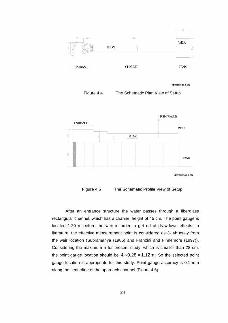
Figure 4.4 The Schematic Plan View of Setup
FLOW
WEIR
TANK
ENTRANCE
dimensions are in cm.
POINT GAUGE
Figure 4.5 The Schematic Profile View of Setup
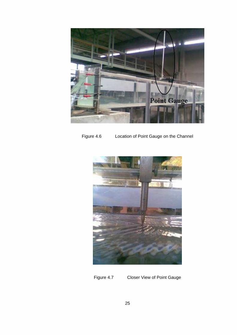
After an entrance structure the water passes through a fiberglass
rectangular channel, which has a channel height of 45 cm. The point gauge is
located 1.20 m before the weir in order to get rid of drawdown effects. In
literature, the effective measurement point is considered as 3- 4h away from
the weir location (Subramanya (1986) and Franzini and Finnemore (1997)).
Considering the maximum h for present study, which is smaller than 28 cm,
the point gauge location should be m1212804 .. =× . So the selected point
gauge location is appropriate for this study. Point gauge accuracy is 0.1 mm
along the centerline of the approach channel (Figure 4.6).
25
Figure 4.6 Location of Point Gauge on the Channel
Figure 4.7 Closer View of Point Gauge
26
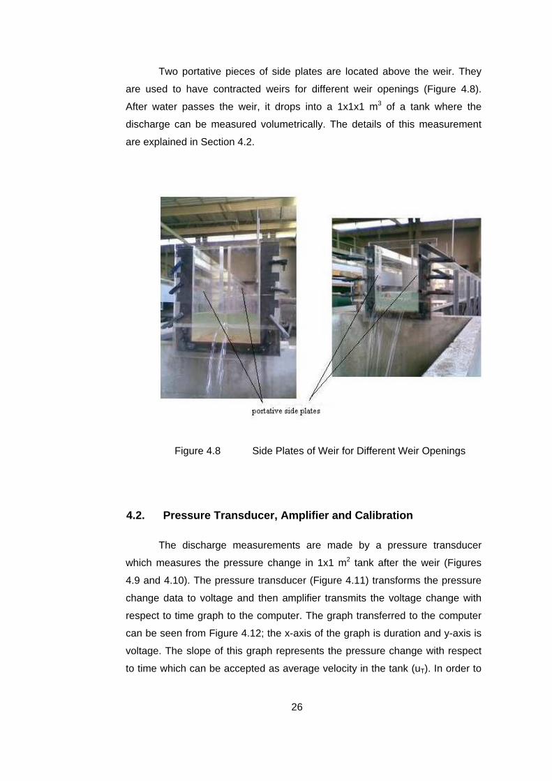
Two portative pieces of side plates are located above the weir. They
are used to have contracted weirs for different weir openings (Figure 4.8).
After water passes the weir, it drops into a 1x1x1 m3 of a tank where the
discharge can be measured volumetrically. The details of this measurement
are explained in Section 4.2.
Figure 4.8 Side Plates of Weir for Different Weir Openings
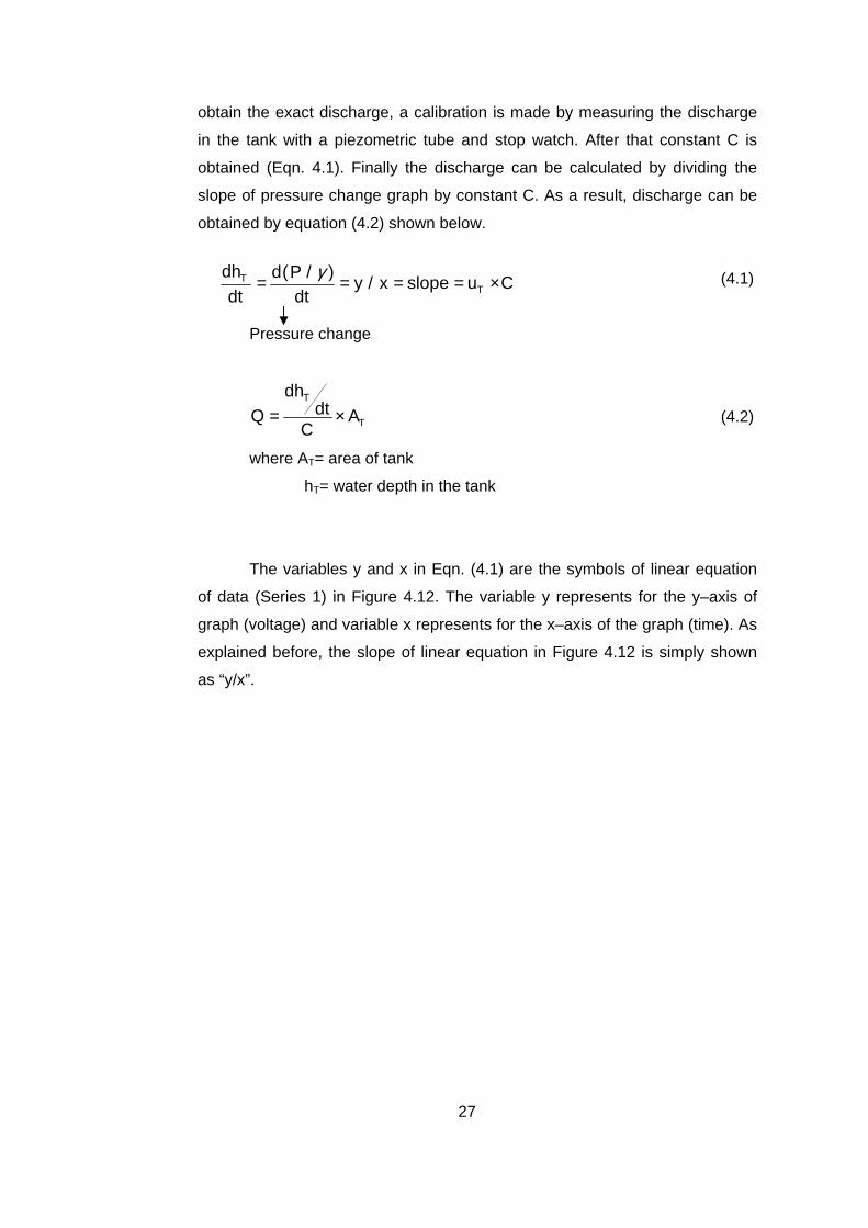
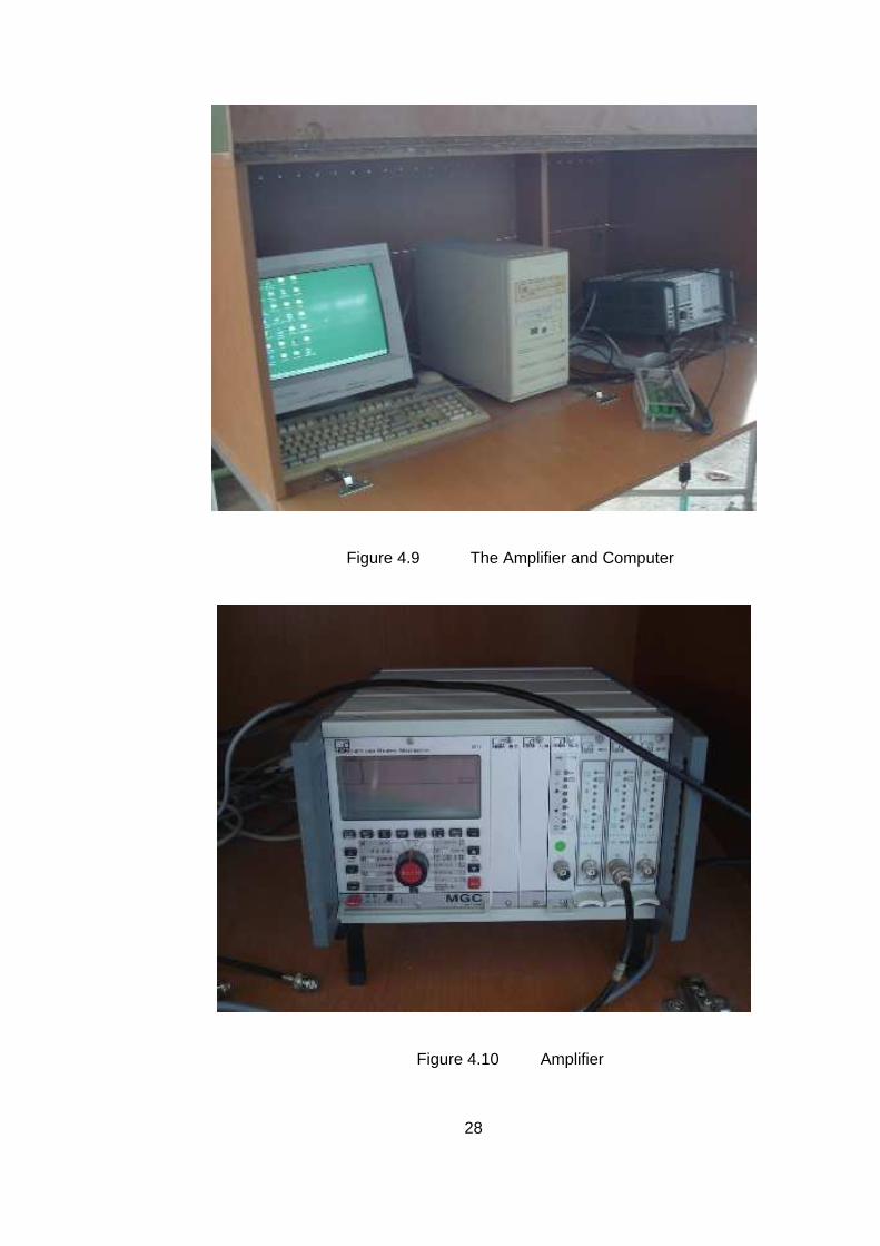
4.2. Pressure Transducer, Amplifier and Calibration
The discharge measurements are made by a pressure transducer
which measures the pressure change in 1x1 m2 tank after the weir (Figures
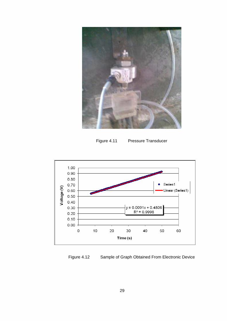
4.9 and 4.10). The pressure transducer (Figure 4.11) transforms the pressure
change data to voltage and then amplifier transmits the voltage change with
respect to time graph to the computer. The graph transferred to the computer
can be seen from Figure 4.12; the x-axis of the graph is duration and y-axis is
voltage. The slope of this graph represents the pressure change with respect
to time which can be accepted as average velocity in the tank (uT). In order to
27
obtain the exact discharge, a calibration is made by measuring the discharge
in the tank with a piezometric tube and stop watch. After that constant C is
obtained (Eqn. 4.1). Finally the discharge can be calculated by dividing the
slope of pressure change graph by constant C. As a result, discharge can be
obtained by equation (4.2) shown below.
(4.1)
Pressure change
T
T
AC
dtdh
Q ×= (4.2)
where AT= area of tank
hT= water depth in the tank
The variables y and x in Eqn. (4.1) are the symbols of linear equation
of data (Series 1) in Figure 4.12. The variable y represents for the y–axis of
graph (voltage) and variable x represents for the x–axis of the graph (time). As
explained before, the slope of linear equation in Figure 4.12 is simply shown
as “y/x”.
Cuslopex/ydt
)/P(ddt
dhT
T ×==== γ
28
Figure 4.9 The Amplifier and Computer
Figure 4.10 Amplifier
29
Figure 4.11 Pressure Transducer
Figure 4.12 Sample of Graph Obtained From Electronic Device
30
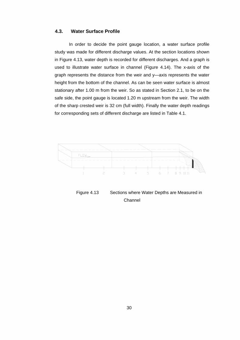
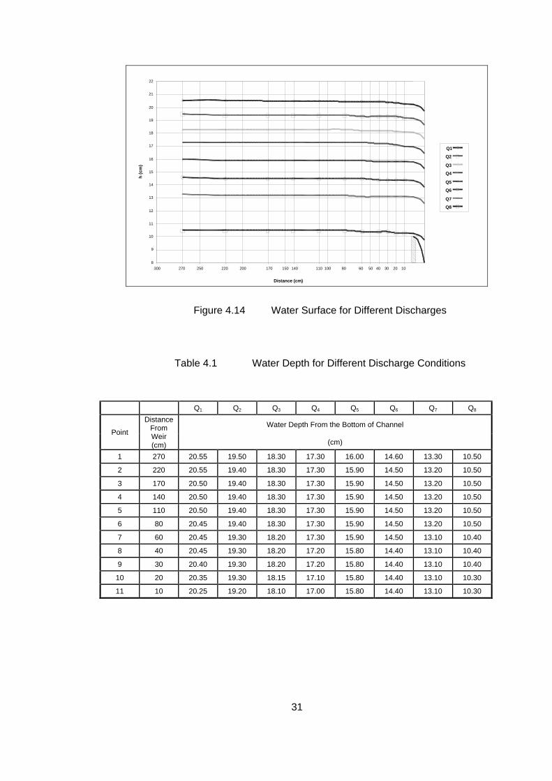
4.3. Water Surface Profile
In order to decide the point gauge location, a water surface profile
study was made for different discharge values. At the section locations shown
in Figure 4.13, water depth is recorded for different discharges. And a graph is
used to illustrate water surface in channel (Figure 4.14). The x-axis of the
graph represents the distance from the weir and y—axis represents the water
height from the bottom of the channel. As can be seen water surface is almost
stationary after 1.00 m from the weir. So as stated in Section 2.1, to be on the
safe side, the point gauge is located 1.20 m upstream from the weir. The width
of the sharp crested weir is 32 cm (full width). Finally the water depth readings
for corresponding sets of different discharge are listed in Table 4.1.
Figure 4.13 Sections where Water Depths are Measured in
Channel
31
1050100150200250300
Distance (cm)
Q1
Q2
Q3
Q4
Q5
Q6
Q7
Q8
2030406080110140170220270
8
9
10
11
12
13
14
15
16
17
18
19
20
21
22
h (c
m)
Figure 4.14 Water Surface for Different Discharges
Table 4.1 Water Depth for Different Discharge Conditions
Q1 Q2 Q3 Q4 Q5 Q6 Q7 Q8
Point
Distance From Weir (cm)
Water Depth From the Bottom of Channel
(cm)
1 270 20.55 19.50 18.30 17.30 16.00 14.60 13.30 10.50
2 220 20.55 19.40 18.30 17.30 15.90 14.50 13.20 10.50
3 170 20.50 19.40 18.30 17.30 15.90 14.50 13.20 10.50
4 140 20.50 19.40 18.30 17.30 15.90 14.50 13.20 10.50
5 110 20.50 19.40 18.30 17.30 15.90 14.50 13.20 10.50
6 80 20.45 19.40 18.30 17.30 15.90 14.50 13.20 10.50
7 60 20.45 19.30 18.20 17.30 15.90 14.50 13.10 10.40
8 40 20.45 19.30 18.20 17.20 15.80 14.40 13.10 10.40
9 30 20.40 19.30 18.20 17.20 15.80 14.40 13.10 10.40
10 20 20.35 19.30 18.15 17.10 15.80 14.40 13.10 10.30
11 10 20.25 19.20 18.10 17.00 15.80 14.40 13.10 10.30
32
5. CHAPTER 5
RESULTS AND DISCUSSION
5.1. Introduction
In this chapter, the results of experiments and comparison of the
results with previous works are discussed in detail.
First of all, in section 5.1.1 experiments for full width sharp crested weir
of different weir height are discussed. The weir height that is free from bottom
boundary effects is chosen to be the constant weir height for the rest of the
study. Then after determining a fixed weir height, experiments are continued
for different weir openings from full width to slit weir. By changing weir width,
the flow characteristics are observed and a discharge equation is tried to be
found. The details of the second part of the experimental work are drawn out
in sections 5.1.2, 5.2 and 5.3.
33
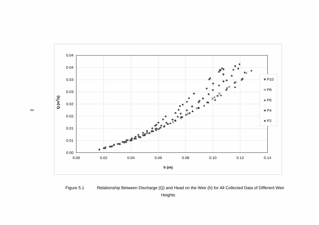
5.1.1. Experimental Works for Different Weir Height s
The selection of constant weir height is accomplished after making
several experimental studies with different weir heights. Experiments are
carried out for 5 different weir heights; 2, 4, 6, 8 and 10 cm for full width
openings. In Figure 5.1; P10, P8, P6, P4 and P2 correspond to weir heights of
10, 8, 6, 4 and 2 cm, respectively. And each symbol represents the different
data group. As can be seen from Figure 5.1, after P = 6 cm, there seems no
change in the variations of Q with h, compared to 8 and 10 cm. However, 2
and 4 cm of weir heights differ from each and all other. Hence, it can be
concluded that for the range of the experiments that were carried out, the
selection of the weir height to be 10 cm will make the effect of bottom
boundary diminish. So, the discharge coefficient, Cd will become independent
of h/P.
3
0.00
0.01
0.01
0.02
0.02
0.03
0.03
0.04
0.04
0.00 0.02 0.04 0.06 0.08 0.10 0.12 0.14
h (m)
Q (
m3 /s
)
P10
P8
P6
P4
P2
Figure 5.1 Relationship Between Discharge (Q) and Head on the Weir (h) for All Collected Data of Different Weir
Heights
35
5.1.2. Experimental Works for Different Weir Openin gs
Experiments are continued after determining a constant weir height of
10 cm. Different weir openings are investigated hydraulically and the results of
this study are explained below.
If two figures (Figure 5.2 and Figure 5.3) are compared regarding the
data points, Figure 5.2 shows that as the discharge increases for a specified
weir width, the water head over the weir obtained are not reliable due to
fluctuation in the channel. For each weir width (b), the outlier data differ from
each other. In other words; each weir width has its own measurable spectrum,
which gives more reliable results. In Figure 5.3 and throughout the whole
calculations the outlier data points are not considered. The data considered
are shown in Figure 5.3 and the range of the experimental data is listed in
Table 5.1.
The weir width ranges were selected in order to cover a spectrum from
slit weir to full width weir. Weir height is constant throughout the whole
experiments, which is 10 cm as can be seen from Table 5.1. Discharge is
changing from 0.00023 m3/s (0.23 lt/s) to 0.05204 m3/s (52.04 lt/s) which
covers a wide spectrum. Water head on the weir is not below 2 cm in order to
get rid of aeration problem and get reliable discharge measurements. In
addition to measured variables, calculated values such as h/b, h/P, b/B are
also shown in Table 5.1.
3
0.000
0.005
0.010
0.015
0.020
0.025
0.030
0.035
0.040
0.045
0.050
0.055
0.060
0.065
0.070
0.00 0.02 0.04 0.06 0.08 0.10 0.12 0.14 0.16 0.18 0.20 0.22 0.24 0.26 0.28 0.30
h (m)
Q (
m3 /s
)b2
b4
b6
b8
b10
b12
b14
b16
b18
b20
b22
b24
b26
b28
b30
b32
Figure 5.2 Relationship Between Discharge (Q) and Head on the Weir (h) for All Collected Data
3
0.000
0.005
0.010
0.015
0.020
0.025
0.030
0.035
0.040
0.045
0.050
0.055
0.060
0.065
0.070
0.00 0.02 0.04 0.06 0.08 0.10 0.12 0.14 0.16 0.18 0.20 0.22 0.24 0.26 0.28 0.30
h (m)
Q(m
3 /s)
b2
b4
b6
b8
b10
b12
b14
b16
b18
b20
b22
b24
b26
b28
b30
b32
Figure 5.3 Relationship Between Discharge (Q) and Head on the Weir (h) for Collected Data Excluding Outliers
3
Table 5.1 Measured and Calculated Ranges of Experimental Process
b (m) P (m) Qmin (m3/s)
Qmax (m3/s)
hmin
(m) hmax
(m) h/bmin h/bmax h/Pmin h/Pmax b/B
0.02 0.10 0.00023 0.00578 0.0317 0.2796 1.59 13.98 0.32 2.80 0.0625 0.04 0.10 0.00025 0.01071 0.0217 0.2732 0.54 6.83 0.22 2.73 0.1250 0.06 0.10 0.00043 0.01624 0.0229 0.2772 0.38 4.62 0.23 2.77 0.1875 0.08 0.10 0.00067 0.02145 0.0262 0.2760 0.33 3.45 0.26 2.76 0.2500 0.10 0.10 0.00071 0.02687 0.0233 0.2757 0.23 2.76 0.23 2.76 0.3125 0.12 0.10 0.00081 0.03130 0.0217 0.2695 0.18 2.25 0.22 2.70 0.3750 0.14 0.10 0.00086 0.03780 0.0208 0.2739 0.15 1.96 0.21 2.74 0.4375 0.16 0.10 0.00134 0.04348 0.0256 0.2730 0.16 1.71 0.26 2.73 0.5000 0.18 0.10 0.00146 0.04418 0.0253 0.2515 0.14 1.40 0.25 2.52 0.5625 0.20 0.10 0.00165 0.04673 0.0256 0.2421 0.13 1.21 0.26 2.42 0.6250 0.22 0.10 0.00140 0.04963 0.0209 0.2323 0.09 1.06 0.21 2.32 0.6875 0.24 0.10 0.00129 0.04871 0.0179 0.2140 0.07 0.89 0.18 2.14 0.7500 0.26 0.10 0.00187 0.05204 0.0224 0.2078 0.09 0.80 0.22 2.08 0.8125 0.28 0.10 0.00153 0.05074 0.0181 0.1897 0.06 0.68 0.18 1.90 0.8750 0.30 0.10 0.00211 0.05069 0.0220 0.1810 0.07 0.60 0.22 1.81 0.9375 0.32 0.10 0.00223 0.05183 0.0214 0.1721 0.07 0.54 0.21 1.72 1.0000
39
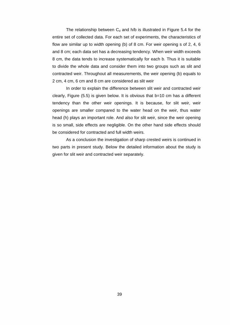
The relationship between Cd and h/b is illustrated in Figure 5.4 for the
entire set of collected data. For each set of experiments, the characteristics of
flow are similar up to width opening (b) of 8 cm. For weir opening s of 2, 4, 6
and 8 cm; each data set has a decreasing tendency. When weir width exceeds
8 cm, the data tends to increase systematically for each b. Thus it is suitable
to divide the whole data and consider them into two groups such as slit and
contracted weir. Throughout all measurements, the weir opening (b) equals to
2 cm, 4 cm, 6 cm and 8 cm are considered as slit weir
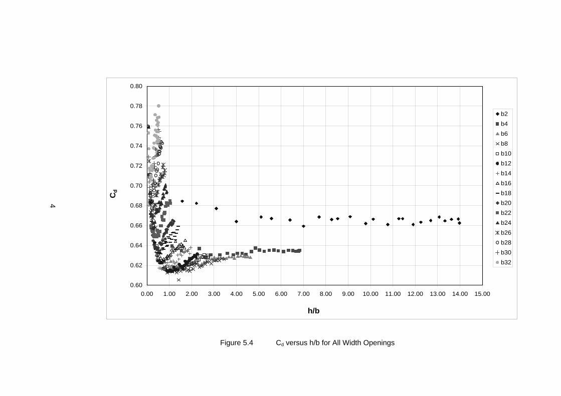
In order to explain the difference between slit weir and contracted weir
clearly, Figure (5.5) is given below. It is obvious that b=10 cm has a different
tendency than the other weir openings. It is because, for slit weir, weir
openings are smaller compared to the water head on the weir, thus water
head (h) plays an important role. And also for slit weir, since the weir opening
is so small, side effects are negligible. On the other hand side effects should
be considered for contracted and full width weirs.
As a conclusion the investigation of sharp crested weirs is continued in
two parts in present study. Below the detailed information about the study is
given for slit weir and contracted weir separately.
4
0.60
0.62
0.64
0.66
0.68
0.70
0.72
0.74
0.76
0.78
0.80
0.00 1.00 2.00 3.00 4.00 5.00 6.00 7.00 8.00 9.00 10.00 11.00 12.00 13.00 14.00 15.00
h/b
Cd
b2
b4
b6
b8
b10
b12
b14
b16
b18
b20
b22
b24
b26
b28
b30
b32
Figure 5.4 Cd versus h/b for All Width Openings
4
0.58
0.59
0.60
0.61
0.62
0.63
0.64
0.65
0.66
0.67
0.68
0.69
0.70
0.71
0.72
0.73
0.74
0.75
0.00 1.00 2.00 3.00 4.00 5.00 6.00 7.00 8.00 9.00 10.00 11.00 12.00 13.00 14.00 15.00
h/b
Cd
b2
b4
b6
b8
b10
Figure 5.5 Difference between Slit and Contracted Weir
42
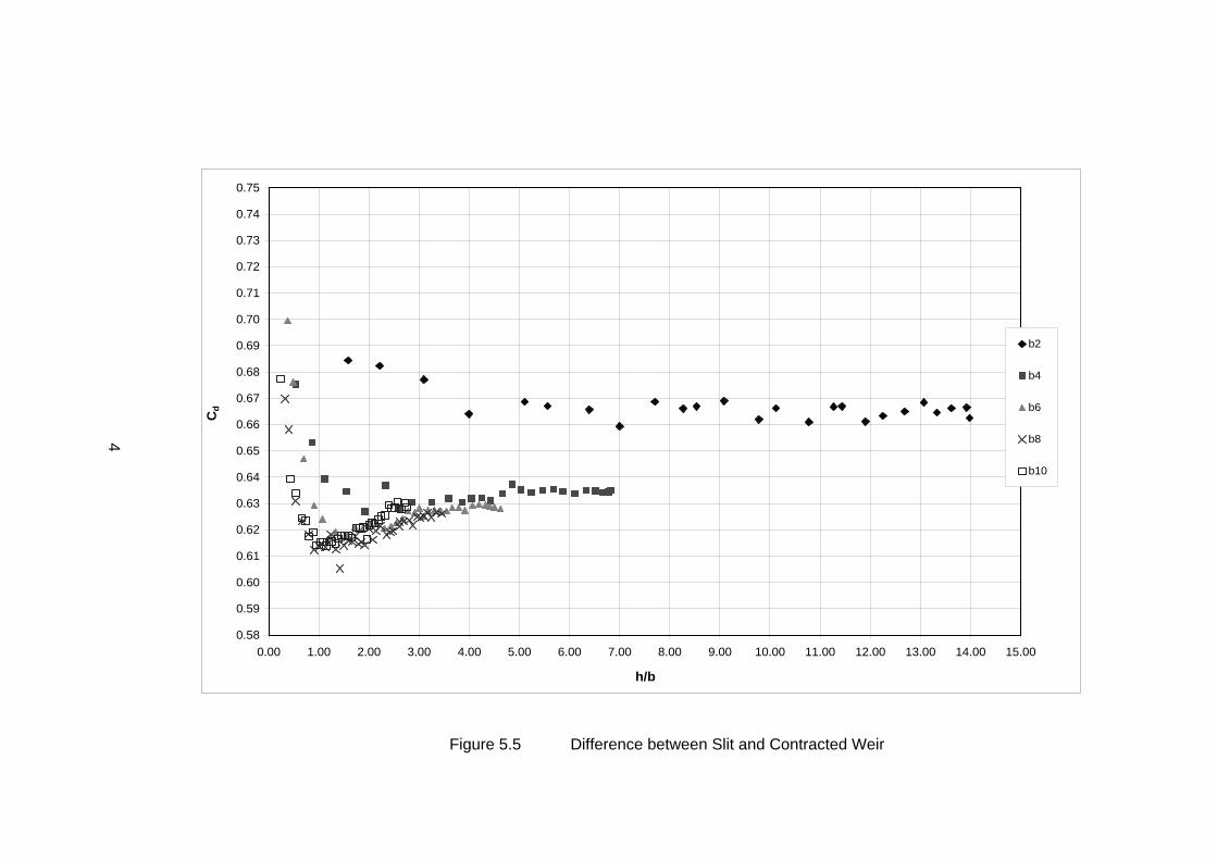
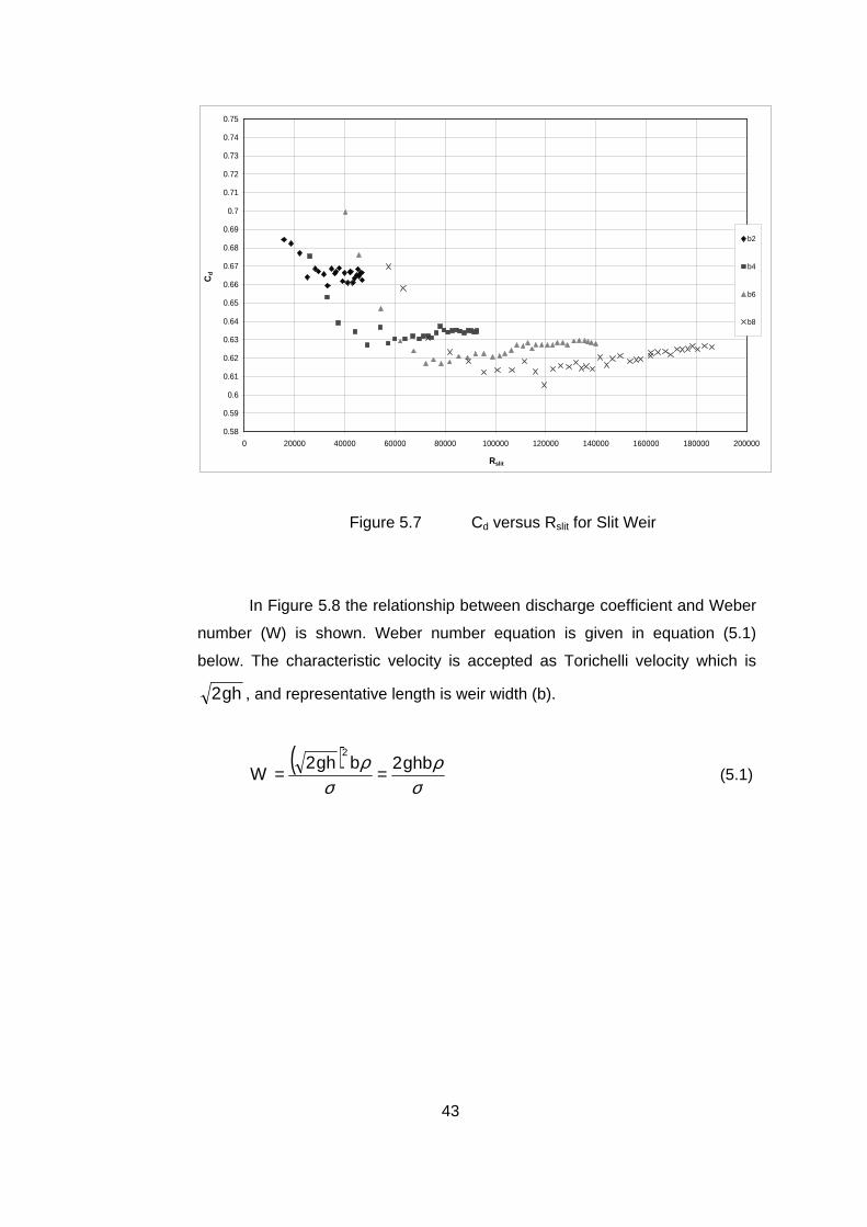
5.2. Slit Weir
A sharp crested weir having a weir width between 2 cm and 8 cm is
considered as a slit weir. It should be mentioned that 8 cm of weir width in a
32 cm wide channel corresponds to 1/4 of the channel width. It can be
concluded that a weir of b ≤ B/4 is considered as slit weir. Below the present
slit weir data is shown in Figure 5.6 and Figure 5.7. Figure 5.6 represents the
relationship between Cd and h/b and Figure 5.7 represents the relationship
between Cd and Rslit.
The Reynolds number considered for slit weir is given in Eqn (3.11).
For slit weirs, the characteristic velocity is accepted as Torichelli velocity which
is gh2 and weir width (b) is used for length parameter.
Rslit= ν
b)gh2( (3.11)
0.58
0.59
0.60
0.61
0.62
0.63
0.64
0.65
0.66
0.67
0.68
0.69
0.70
0.71
0.72
0.73
0.74
0.75
0.00 1.00 2.00 3.00 4.00 5.00 6.00 7.00 8.00 9.00 10.00 11.00 12.00 13.00 14.00 15.00
h/b
Cd
b2
b4
b6
b8
Figure 5.6 Cd versus h/b for Slit Weir
43
0.58
0.59
0.6
0.61
0.62
0.63
0.64
0.65
0.66
0.67
0.68
0.69
0.7
0.71
0.72
0.73
0.74
0.75
0 20000 40000 60000 80000 100000 120000 140000 160000 180000 200000
Rslit
Cd
b2
b4
b6
b8
Figure 5.7 Cd versus Rslit for Slit Weir
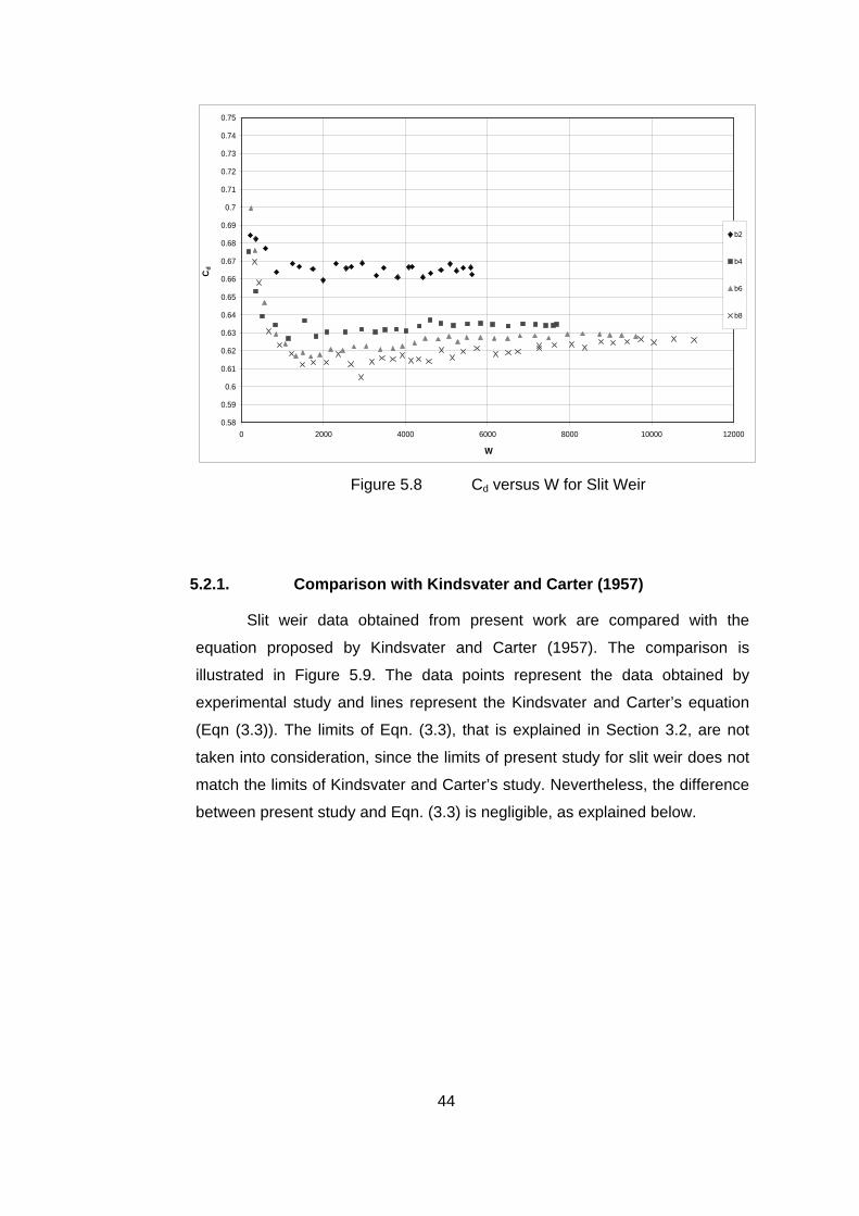
In Figure 5.8 the relationship between discharge coefficient and Weber
number (W) is shown. Weber number equation is given in equation (5.1)
below. The characteristic velocity is accepted as Torichelli velocity which is
gh2 , and representative length is weir width (b).
( )σ
ρσ
ρ ghb2bgh2W
2
== (5.1)
44
0.58
0.59
0.6
0.61
0.62
0.63
0.64
0.65
0.66
0.67
0.68
0.69
0.7
0.71
0.72
0.73
0.74
0.75
0 2000 4000 6000 8000 10000 12000
W
Cd
b2
b4
b6
b8
Figure 5.8 Cd versus W for Slit Weir
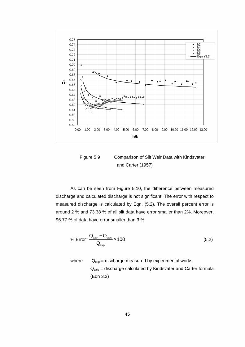
5.2.1. Comparison with Kindsvater and Carter (1957)
Slit weir data obtained from present work are compared with the
equation proposed by Kindsvater and Carter (1957). The comparison is
illustrated in Figure 5.9. The data points represent the data obtained by
experimental study and lines represent the Kindsvater and Carter’s equation
(Eqn (3.3)). The limits of Eqn. (3.3), that is explained in Section 3.2, are not
taken into consideration, since the limits of present study for slit weir does not
match the limits of Kindsvater and Carter’s study. Nevertheless, the difference
between present study and Eqn. (3.3) is negligible, as explained below.
45
0.58
0.59
0.60
0.61
0.62
0.63
0.64
0.65
0.66
0.67
0.68
0.69
0.70
0.71
0.72
0.73
0.74
0.75
0.00 1.00 2.00 3.00 4.00 5.00 6.00 7.00 8.00 9.00 10.00 11.00 12.00 13.00
h/b
Cd
b2b4b6b8Eqn. (3.3)_
Figure 5.9 Comparison of Slit Weir Data with Kindsvater
and Carter (1957)
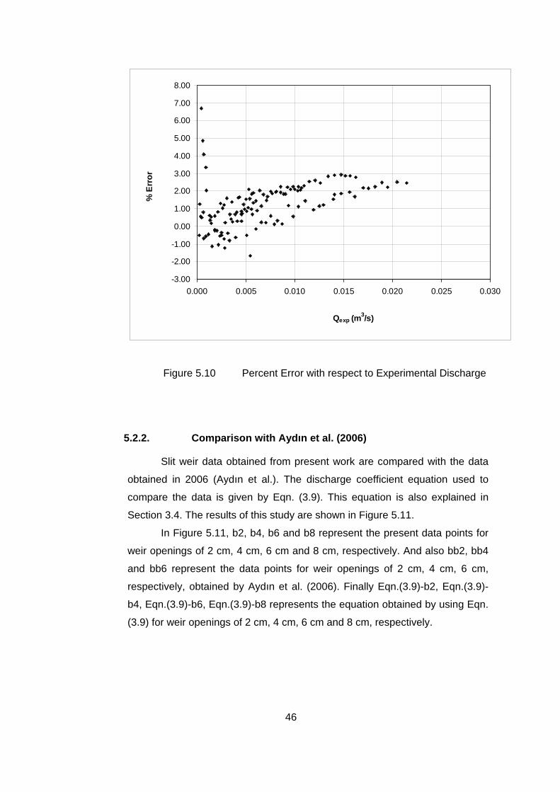
As can be seen from Figure 5.10, the difference between measured
discharge and calculated discharge is not significant. The error with respect to
measured discharge is calculated by Eqn. (5.2). The overall percent error is
around 2 % and 73.38 % of all slit data have error smaller than 2%. Moreover,
96.77 % of data have error smaller than 3 %.
% Error= 100Q
exp
calcexp ×−
(5.2)
where Qexp = discharge measured by experimental works
Qcalc = discharge calculated by Kindsvater and Carter formula
(Eqn 3.3)
46
-3.00
-2.00
-1.00
0.00
1.00
2.00
3.00
4.00
5.00
6.00
7.00
8.00
0.000 0.005 0.010 0.015 0.020 0.025 0.030
Qexp (m3/s)
% E
rror
Figure 5.10 Percent Error with respect to Experimental Discharge
5.2.2. Comparison with Aydın et al. (2006)
Slit weir data obtained from present work are compared with the data
obtained in 2006 (Aydın et al.). The discharge coefficient equation used to
compare the data is given by Eqn. (3.9). This equation is also explained in
Section 3.4. The results of this study are shown in Figure 5.11.
In Figure 5.11, b2, b4, b6 and b8 represent the present data points for
weir openings of 2 cm, 4 cm, 6 cm and 8 cm, respectively. And also bb2, bb4
and bb6 represent the data points for weir openings of 2 cm, 4 cm, 6 cm,
respectively, obtained by Aydın et al. (2006). Finally Eqn.(3.9)-b2, Eqn.(3.9)-
b4, Eqn.(3.9)-b6, Eqn.(3.9)-b8 represents the equation obtained by using Eqn.
(3.9) for weir openings of 2 cm, 4 cm, 6 cm and 8 cm, respectively.
47
0.55
0.6
0.65
0.7
0.75
0.8
0.85
0.9
0 20000 40000 60000 80000 100000 120000 140000 160000 180000 200000
Rslit
Cd
b2b4b6b8bb2bb4bb6Eqn.(3.9)-b2Eqn.(3.9)-b4Eqn.(3.9)-b6Eqn.(3.9)-b8_
Figure 5.11 Comparison of New Experimental Data, Old
Experimental Data (Aydın et al. (2006)) and
Slit Weir Equation (Eqn. (3.9))
Different from previous study made in 2006 by Aydın et al., the study is
enhanced and measured discharge values become greater than the previous
study. Hence, greater Reynolds numbers are obtained in the present study.
Considering the relation between Cd and Reynolds number; the old data for b
is 2 cm, the maximum Reynolds number is approximately 45000; for b is 4 cm,
it is 70000 and for b is 6 cm maximum Reynolds number is around 90000. On
the other hand, for the present study Reynolds number approaches to 140000
for b equals to 6 cm. Thus different behavior of Cd as a function of R is
observed. It is seen that as R gets larger, for different weir widths, the
discharge coefficient approaches to different values asymptotically rather than
one asymptotic value as obtained before by Aydın et al. (2006). So an
improved study is needed for rectangular slit weirs.
48
The percent error is calculated by Eqn. (5.2), Qcalc is the discharge
calculated by Eqn (3.9)and Qexp is the present measured discharge by
experimental works. As can be seen from the Figure 5.12, the error with
respect to measured discharge is acceptable since the maximum error is
around 8 %.
The overall percent error is between 4 % to -3 %, disregarding few data
points. And also 62.25 % of all slit data have error smaller than 2 %, whereas
92.31 % of all slit data have error smaller than 3 %. Besides that, the study
made by Aydın et al. (2006) has relative error within 2 % for 89 % of the total
data.
-8.000
-7.000
-6.000
-5.000
-4.000
-3.000
-2.000
-1.000
0.000
1.000
2.000
3.000
4.000
5.000
0 0.002 0.004 0.006 0.008 0.01 0.012 0.014 0.016 0.018 0.02 0.022 0.024
Qexp (m3/s)
% E
rror
Figure 5.12 Percent Error with respect to Experimental Discharge
and Eqn. (3.6)
49
5.3. Contracted Weir
The sharp crested weirs having widths greater or equal to 10 cm are
considered as contracted weirs as explained in Section 5.1.
For contracted weirs the definition of Reynolds number is revised and a
new form of Reynolds number is used. In the definition of Reynolds number
(R) for contracted weirs, the square root of flow area is accepted as a
characteristic length for contracted weir. Because for this type of weirs, both
weir width and water head are important.
Rcontracted= ν)bh()gh(2
(5.3)
5.3.1. Comparison with Rehbock (1929)
As stated, Rehbock made a study for full width sharp crested weirs.
Therefore the comparison is made only for full width weir data obtained. Below
the present data and Rehbock study is compared (Fig. 5.13 ).
0.60
0.65
0.70
0.75
0.80
0.85
0.90
0 100000 200000 300000 400000 500000 600000
Rcontracted
Cd
exp
Eqn. (3.1)
Figure 5.13 Comparison of Contracted Weir Data with Eqn. (3.1)
50
The percent error given in Figure 5.16 is calculated by Eqn. (5.2), Qcalc
is the discharge calculated by Eqn (3.1)and Qexp is the present measured
discharge by experimental works. As can be seen from the Figure 5.14, the
relative error is between +18 % and – 2 %. In addition to this, 44.12 % of all
contracted data have error smaller than 5%. Moreover, 88.24 % of data have
error smaller than 10 %.
-2.00
0.00
2.00
4.00
6.00
8.00
10.00
12.00
14.00
16.00
18.00
0.00 0.01 0.02 0.03 0.04 0.05 0.06
Qexp (m3/s)
% E
rror
r
Figure 5.14 Percent Error with respect to Experimental Discharge
and Eqn. (3.1)
51
5.3.2. Comparison with Kindsvater and Carter (1957)
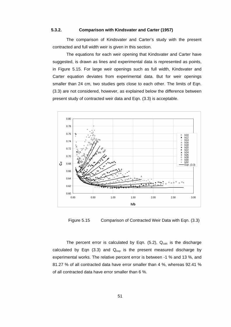
The comparison of Kindsvater and Carter’s study with the present
contracted and full width weir is given in this section.
The equations for each weir opening that Kindsvater and Carter have
suggested, is drawn as lines and experimental data is represented as points,
in Figure 5.15. For large weir openings such as full width, Kindsvater and
Carter equation deviates from experimental data. But for weir openings
smaller than 24 cm, two studies gets close to each other. The limits of Eqn.
(3.3) are not considered, however, as explained below the difference between
present study of contracted weir data and Eqn. (3.3) is acceptable.
0.60
0.62
0.64
0.66
0.68
0.70
0.72
0.74
0.76
0.78
0.80
0.00 0.50 1.00 1.50 2.00 2.50 3.00
h/b
Cd
b10b12b14b16b18b20b22b24b26b28b30b32Eqn. (3.3)_
Figure 5.15 Comparison of Contracted Weir Data with Eqn. (3.3)
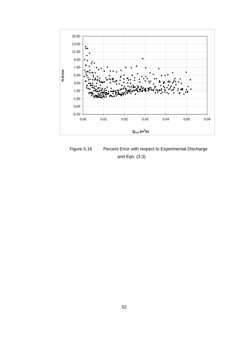
The percent error is calculated by Eqn. (5.2), Qcalc is the discharge
calculated by Eqn (3.3) and Qexp is the present measured discharge by
experimental works. The relative percent error is between -1 % and 13 %, and
81.27 % of all contracted data have error smaller than 4 %, whereas 92.41 %
of all contracted data have error smaller than 6 %.
52
-5.00
-3.00
-1.00
1.00
3.00
5.00
7.00
9.00
11.00
13.00
15.00
0.00 0.01 0.02 0.03 0.04 0.05 0.06
Qexp (m3/s)
% E
rror
Figure 5.16 Percent Error with respect to Experimental Discharge
and Eqn. (3.3)
53
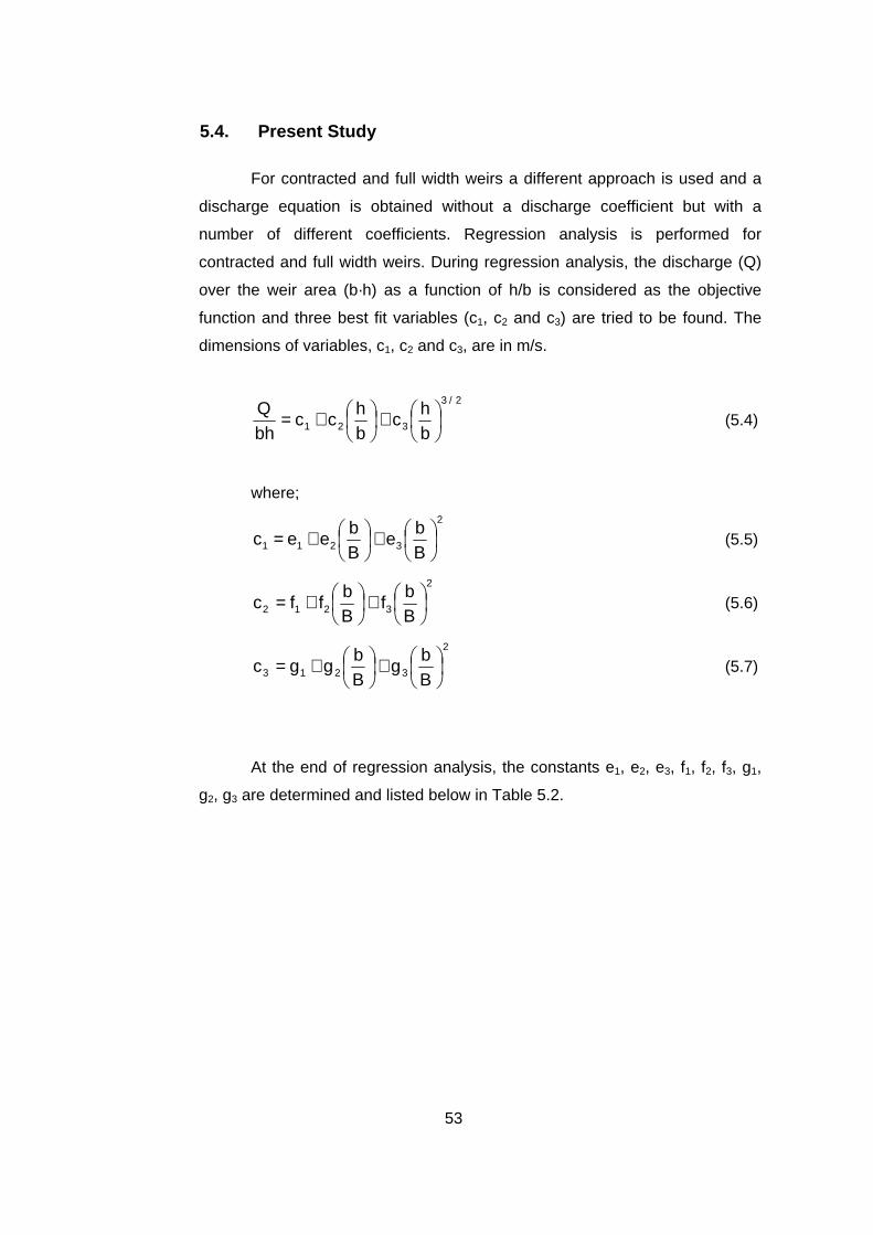
5.4. Present Study
For contracted and full width weirs a different approach is used and a
discharge equation is obtained without a discharge coefficient but with a
number of different coefficients. Regression analysis is performed for
contracted and full width weirs. During regression analysis, the discharge (Q)
over the weir area (b·h) as a function of h/b is considered as the objective
function and three best fit variables (c1, c2 and c3) are tried to be found. The
dimensions of variables, c1, c2 and c3, are in m/s.
23
321
/
bh
cbh
ccbhQ
+
+= (5.4)
where;
2
3211
+
+=Bb
eBb
eec (5.5)
2
3212
+
+=Bb
fBb
ffc (5.6)
2
3213
+
+=Bb
gBb
ggc (5.7)
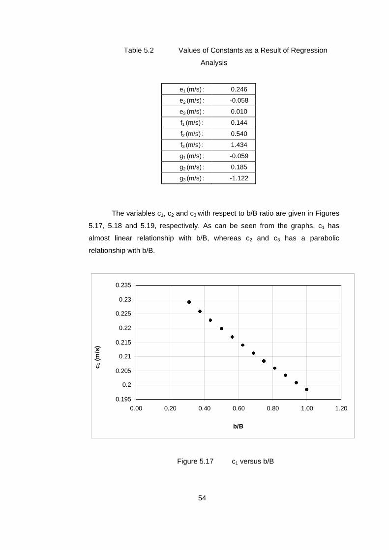
At the end of regression analysis, the constants e1, e2, e3, f1, f2, f3, g1,
g2, g3 are determined and listed below in Table 5.2.
54
Table 5.2 Values of Constants as a Result of Regression
Analysis
e1 (m/s) : 0.246
e2 (m/s) : -0.058
e3 (m/s) : 0.010
f1 (m/s) : 0.144
f2 (m/s) : 0.540
f3 (m/s) : 1.434
g1 (m/s) : -0.059
g2 (m/s) : 0.185
g3 (m/s) : -1.122
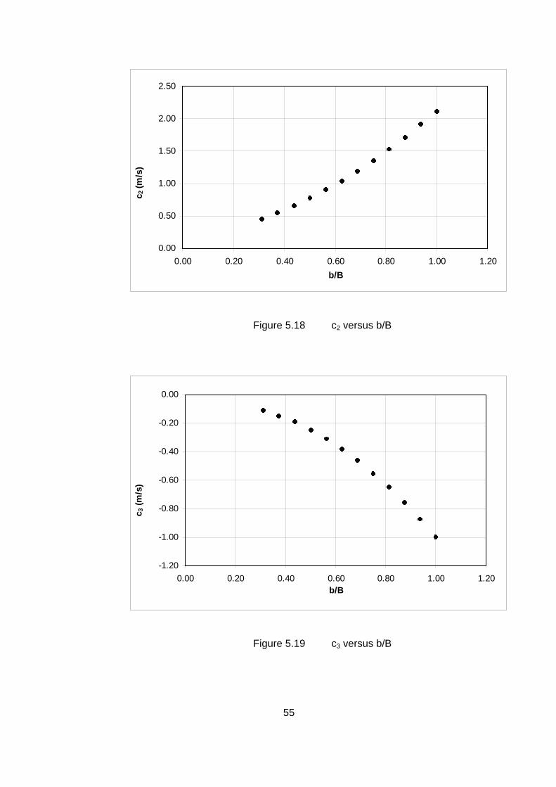
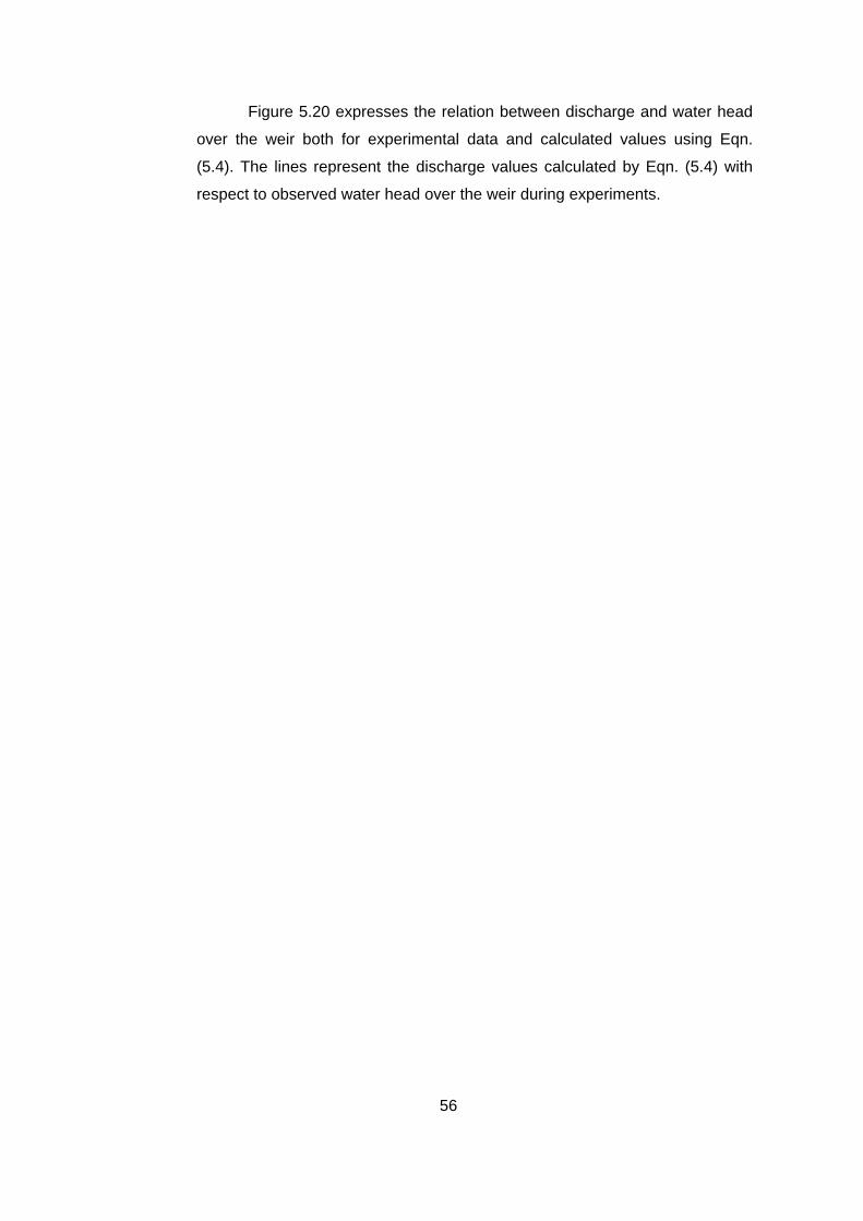
The variables c1, c2 and c3 with respect to b/B ratio are given in Figures
5.17, 5.18 and 5.19, respectively. As can be seen from the graphs, c1 has
almost linear relationship with b/B, whereas c2 and c3 has a parabolic
relationship with b/B.
0.195
0.2
0.205
0.21
0.215
0.22
0.225
0.23
0.235
0.00 0.20 0.40 0.60 0.80 1.00 1.20
b/B
c 1 (
m/s
)
Figure 5.17 c1 versus b/B
55
0.00
0.50
1.00
1.50
2.00
2.50
0.00 0.20 0.40 0.60 0.80 1.00 1.20
b/B
c 2 (m
/s)
Figure 5.18 c2 versus b/B
-1.20
-1.00
-0.80
-0.60
-0.40
-0.20
0.00
0.00 0.20 0.40 0.60 0.80 1.00 1.20b/B
c 3 (
m/s
)
Figure 5.19 c3 versus b/B
56
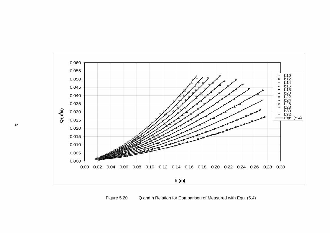
Figure 5.20 expresses the relation between discharge and water head
over the weir both for experimental data and calculated values using Eqn.
(5.4). The lines represent the discharge values calculated by Eqn. (5.4) with
respect to observed water head over the weir during experiments.
5
0.000
0.005
0.010
0.015
0.020
0.025
0.030
0.035
0.040
0.045
0.050
0.055
0.060
0.00 0.02 0.04 0.06 0.08 0.10 0.12 0.14 0.16 0.18 0.20 0.22 0.24 0.26 0.28 0.30
h (m)
Q (m
3 /s)
b10b12b14b16b18b20b22b24b26b28b30b32Eqn. (5.4)12
Figure 5.20 Q and h Relation for Comparison of Measured with Eqn. (5.4)
58
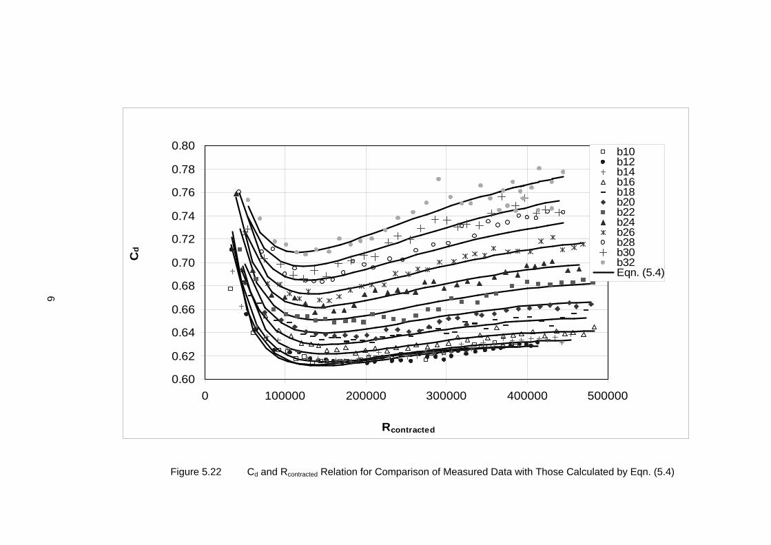
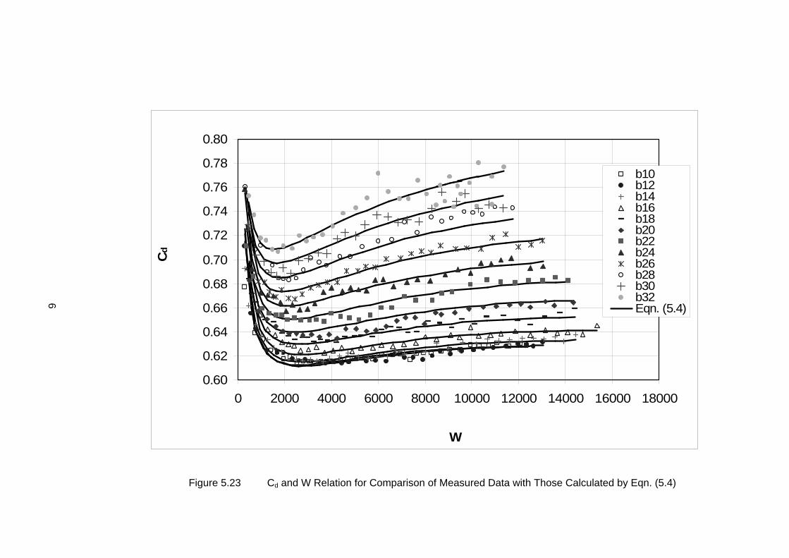
Figure 5.21 gives the comparison of experimental data and calculated
data as Cd versus h/b relation. The relation between Cd and R; Cd and W can
be observed by Figure 5.22 and Figure 5.23, respectively. As can be seen in
Figure 5.22 and 5.23; it is very difficult to fix an equation of discharge
coefficient as a function of Reynolds number and/or Weber number. Weber
number for contracted weir is also calculated by using equation (5.1) like slit
weir.
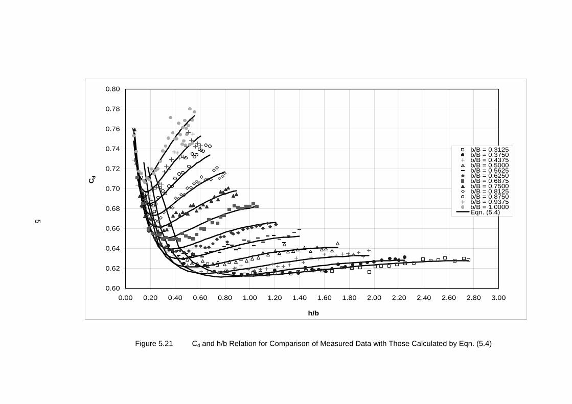
5
0.60
0.62
0.64
0.66
0.68
0.70
0.72
0.74
0.76
0.78
0.80
0.00 0.20 0.40 0.60 0.80 1.00 1.20 1.40 1.60 1.80 2.00 2.20 2.40 2.60 2.80 3.00
h/b
Cd
b/B = 0.3125b/B = 0.3750b/B = 0.4375b/B = 0.5000b/B = 0.5625b/B = 0.6250b/B = 0.6875b/B = 0.7500b/B = 0.8125b/B = 0.8750b/B = 0.9375b/B = 1.0000Eqn. (5.4)_
Figure 5.21 Cd and h/b Relation for Comparison of Measured Data with Those Calculated by Eqn. (5.4)
6
0.60
0.62
0.64
0.66
0.68
0.70
0.72
0.74
0.76
0.78
0.80
0 100000 200000 300000 400000 500000
Rcontracted
Cd
b10b12b14b16b18b20b22b24b26b28b30b32Eqn. (5.4)_
Figure 5.22 Cd and Rcontracted Relation for Comparison of Measured Data with Those Calculated by Eqn. (5.4)
6
0.60
0.62
0.64
0.66
0.68
0.70
0.72
0.74
0.76
0.78
0.80
0 2000 4000 6000 8000 10000 12000 14000 16000 18000
W
Cd
b10b12b14b16b18b20b22b24b26b28b30b32Eqn. (5.4)_
Figure 5.23 Cd and W Relation for Comparison of Measured Data with Those Calculated by Eqn. (5.4)
62
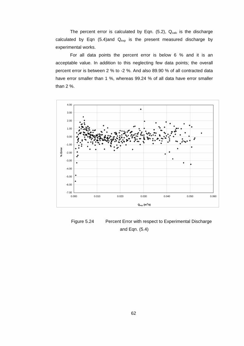
The percent error is calculated by Eqn. (5.2), Qcalc is the discharge
calculated by Eqn (5.4)and Qexp is the present measured discharge by
experimental works.
For all data points the percent error is below 6 % and it is an
acceptable value. In addition to this neglecting few data points; the overall
percent error is between 2 % to -2 %. And also 89.90 % of all contracted data
have error smaller than 1 %, whereas 99.24 % of all data have error smaller
than 2 %.
-7.00
-6.00
-5.00
-4.00
-3.00
-2.00
-1.00
0.00
1.00
2.00
3.00
4.00
0.000 0.010 0.020 0.030 0.040 0.050 0.060
Qexp (m3/s)
% E
rror
Figure 5.24 Percent Error with respect to Experimental Discharge
and Eqn. (5.4)
63
6. CHAPTER 6
CONCLUSION
In the present study, an empirical approach is used for the investigation
of rectangular sharp crested weirs. As indicated in the previous chapters,
experiments are made with a 32 cm width of fiberglass channel and a
rectangular weir for different weir openings from full width weir to slit weir of 2
cm minimum opening.
The conclusions of the analysis of the experimental data are listed
below:
i. For all weir openings below 2 cm of water head over the weir, non-
aerated flow is observed. Thus the minimum water head is 2 cm.
ii. Water surface profile experiments are conducted to determine the
effective measurement location of point gauge, and it is concluded
that the drawdown effect of sharp crested weir is negligible 1.20 m
upstream from the weir location which is greater than 3-4h as given
in literature.
iii. Full width sharp crested rectangular weirs are investigated by
changing the weir height and it is concluded that bottom boundary
effect is negligible for P equals to 6, 8 10 cm. Weir height of 2 and 4
cm is not efficient to investigate the sharp crested rectangular weirs.
As a result weir height of 10 cm is chosen for the rest of the
experiments.
64
iv. Sharp crested rectangular weirs should be considered in two parts
such as; slit weir and contracted weir.
v. Slit weir experimental data results show that the proposed discharge
coefficient equation by Aydın et al. (2006) is reliable. But the equation
(Eqn. 3.9) should be improved for larger values of discharge.
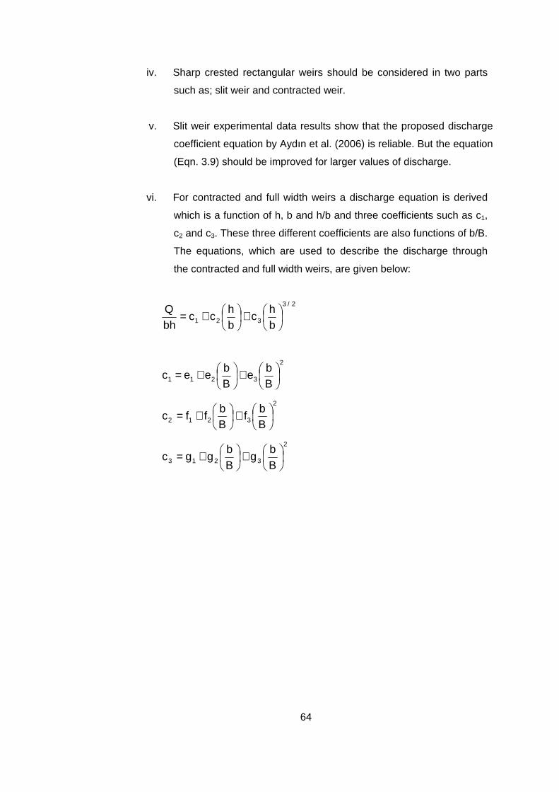
vi. For contracted and full width weirs a discharge equation is derived
which is a function of h, b and h/b and three coefficients such as c1,
c2 and c3. These three different coefficients are also functions of b/B.
The equations, which are used to describe the discharge through
the contracted and full width weirs, are given below:
23
321
/
bh
cbh
ccbhQ
+
+=
2
3211
+
+=Bb
eBb
eec
2
3212
+
+=Bb
fBb
ffc
2
3213
+
+=Bb
gBb
ggc
65
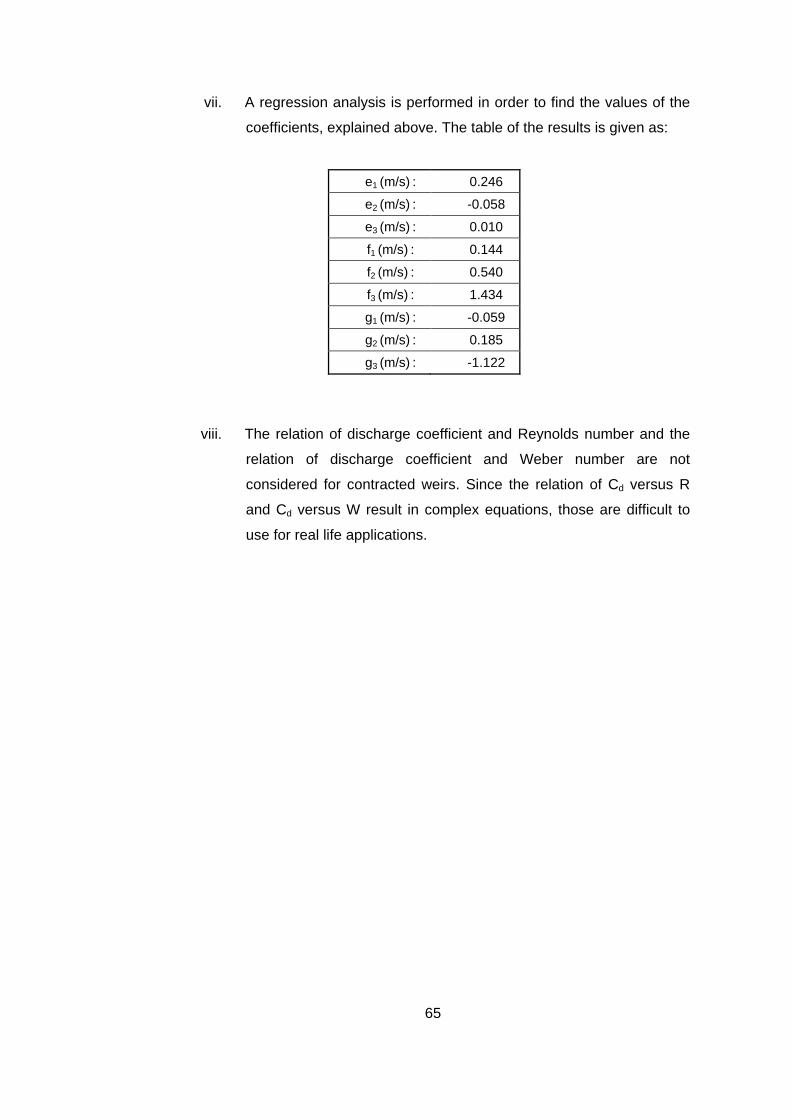
vii. A regression analysis is performed in order to find the values of the
coefficients, explained above. The table of the results is given as:
e1 (m/s) : 0.246
e2 (m/s) : -0.058
e3 (m/s) : 0.010
f1 (m/s) : 0.144
f2 (m/s) : 0.540
f3 (m/s) : 1.434
g1 (m/s) : -0.059
g2 (m/s) : 0.185
g3 (m/s) : -1.122
viii. The relation of discharge coefficient and Reynolds number and the
relation of discharge coefficient and Weber number are not
considered for contracted weirs. Since the relation of Cd versus R
and Cd versus W result in complex equations, those are difficult to
use for real life applications.
66
7. REFERENCES
Aydın, İ., Ger, A. M. and Hınçal, O. (2002). “Measurement of Small
Discharges in Open Channels by Slit Weir.” Journal of Hydraulic Engineering,
Vol. 128, No. 2, 234-237.
Aydın, İ., Altan-Sakarya, A. B. and Ger, A. M. (2006). “Performance of
Slit Weir.” Journal of Hydraulic Engineering, Vol. 132, No. 9, 987-989.
Bos, M. G. (1989). “Discharge Measurement Structures.” International
Institute for Land Reclamation and Improvement, Third Edition, Wageningen,
The Netherlands.
Chow, V. T. (1959). “Open Channel Hydraulics.” McGraw-Hill Book
Company Inc., Newyork.
Coxon, W. F. (1959). “Flow Measurement and Control.” Heywood &
Company Ltd., London.
Franzini, J. B. and Finnemore, E. J. (1997). “Fluid Mechanics with
Engineering Applications.” McGraw-Hill Company Inc.
Henderson, F. M. (1966). “Open Channel Flow.” Prentice-Hall Inc.
Hınçal, O. (2000). “Discharge Coefficient for Slit Weirs.” MSc. Thesis
Department of Civil Engineering, Middle East Technical University, Ankara,
Turkey.
67
Kandaswamy, P. K. and Rouse, H. (1957) “Characteristics of Flow
Over Terminal Weirs and Sills.” Journal of of Hydraulics Division, Vol. 83, No.
4, August, 1-13.
Kinsdvater, C. E. and Cater, R. W. (1957). “Discharge Characteristics
of Rectangular Thin-Plate Weirs.” Journal of Hydraulics Division, Vol. 83, No.
6, December, 1-36.
Munson, B. R., Young, D. F. and Okiishi, T. H. (2002). “Fundamentals
of Fluid Mechanics.” John Wiley & Sons Inc., Newyork, USA.
Subramanya, K. (1986). “Flow in Open Channels.” McGraw-Hill
Publishing Company Limited
Swamee, P. K., (1988). “Generalized Rectangular Weir Equations.”
Journal of Hydraulic Engineering, Vol. 114, No. 8, 945-949.
Ramamurthy, A. S., Tim, U. S. and Rao, M. V. J. (1987). “Flow over
Sharp Crested Plate Weirs.” Journal of Irrigation and Drainage Engineering,
Vol. 113, No. 2, 163-172.
Ramamurthy, A. S., Qu, J., Zhai, C. and Vo, D. (2007). “Multislit Weir
Characteristics.” Journal of Irrigation and Drainage Engineering, Vol. 133, No.
2, 198-200.
Rehbock, T. (1929). “Discussion of ‘Precise Measurements’.” By K. B.
Turner. Trans., ASCE, Vol. 93, 1143-1162.