Experimental Study of Tsunami Generation by Three-Dimensional Rigid Underwater Landslides€¦ · · 2011-05-05Experimental Study of Tsunami Generation by Three-Dimensional Rigid

Experimental Study of Tsunami Generationby Three-Dimensional Rigid Underwater Landslides

François Enet1 and Stéphan T. Grilli, M.ASCE2

Abstract: Large scale, three-dimensional, laboratory experiments are performed to study tsunami generation by rigid underwater land-slides. The main purpose of these experiments is to both gain insight into landslide tsunami generation processes and provide data forsubsequent validation of a three-dimensional numerical model. In each experiment a smooth and streamlined rigid body slides down aplane slope, starting from different initial submergence depths, and generates surface waves. Different conditions of wave nonlinearity anddispersion are generated by varying the model slide initial submergence depth. Surface elevations are measured with capacitance gauges.Runup is measured at the tank axis using a video camera. Landslide acceleration is measured with a microaccelerometer embedded withinthe model slide, and its time of passage is further recorded at three locations down the slope. The repeatability of experiments is verygood. Landslide kinematics is inferred from these measurements and an analytic law of motion is derived, based on which the slide addedmass and drag coefficients are computed. Characteristic distance and time of slide motion, as well as a characteristic tsunami wavelength,are parameters derived from these analyses. Measured wave elevations yield characteristic tsunami amplitudes, which are found to be wellpredicted by empirical equations derived in earlier work, based on two-dimensional numerical computations. The strongly dispersivenature and directionality of tsunamis generated by underwater landslides is confirmed by wave measurements at gauges. Measured coastalrunup is analyzed and found to correlate well with initial slide submergence depth or characteristic tsunami amplitude.

DOI: 10.1061/�ASCE�0733-950X�2007�133:6�442�

CE Database subject headings: Tsunamis; Landslides; Laboratory tests; Wave runup; Surface waves; Experimentation.

Introduction

Except for the large and fortunately less frequent transoceanictsunamis generated by large earthquake, such as the disaster re-cently witnessed in the Indian Ocean �e.g., Titov et al. 2005;Grilli et al. 2007�, underwater landslides represent one of themost dangerous mechanisms for tsunami generation in coastalareas. While tsunamis generated by coseismic displacements aremore often of small amplitude and correlate well with the earth-quake moment magnitude, tsunamis generated by submarinelandslides are only limited by the vertical extent of landslide mo-tion �Murty 1979; Watts 1998�. Moreover, underwater landslidescan be triggered by moderate earthquakes and often occur on thecontinental slope. Hence, these so-called “landslide tsunamis”offer little time for warning local populations. For instance, theconsensus in the scientific community is that the 1998 Papua NewGuinea tsunami, which caused over 2,000 deaths among the localcoastal population, was generated by an underwater slump, itselftriggered by a moderate earthquake of moment magnitudeMs�7.1. �Tappin et al. 2001, 2006; Synolakis et al. 2002�. The

1Engineer, Alkyon Hydraulic Consultancy & Research, P.O. Box 248,8300AE Emmeloord, The Netherlands.

2Professor, Dept. of Ocean Engineering, Univ. of Rhode Island, Nar-ragansett, RI 02882 �corresponding author�. E-mail: [email protected]

Note. Discussion open until April 1, 2008. Separate discussions mustbe submitted for individual papers. To extend the closing date by onemonth, a written request must be filed with the ASCE Managing Editor.The manuscript for this paper was submitted for review and possiblepublication on February 3, 2006; approved on September 30, 2006. Thispaper is part of the Journal of Waterway, Port, Coastal, and OceanEngineering, Vol. 133, No. 6, November 1, 2007. ©ASCE, ISSN 0733-
950X/2007/6-442–454/$25.00.
442 / JOURNAL OF WATERWAY, PORT, COASTAL, AND OCEAN ENGINE

Downloaded 05 May 2011 to 128.175.255.36. Redistrib

large coastal hazard posed by landslide tsunamis justifies the needfor identifying sensitive sites and accurately predicting possiblelandslide tsunami scenarii and amplitudes.

The methods used for predicting landslide tsunami amplitudesare of three main types: �1� laboratory experiments; �2� analyticaldescriptions; and �3� numerical simulations. Whereas laboratoryexperiments can be made quite realistic, they suffer from scaleeffects and are quite costly to implement, which limits the numberof experiments and the relevant parameter space that can be ex-plored. Properly validated numerical models �e.g., Grilli andWatts 1999; Grilli et al. 2002� can advantageously complementexperiments and simulate tsunamis generated by a variety of sub-marine mass failures �SMFs�, of which rigid landslides representone idealized case. Such models have also been used to computetsunami sources for a variety of SMFs and conduct successfulcase studies �Watts et al. 2003, 2005; Days et al. 2005; Ioualalenet al. 2006; Tappin et al. 2006�.

Most of the laboratory experiments and related analytical de-scriptions reported so far have been done for two-dimensional�2D� cases, either represented by solid bodies sliding down aplane slope �e.g., Wiegel 1955; Iwasaki 1982; Heinrich 1992;Watts 1997, 1998, 2000; Watts et al. 2000; Grilli and Watts 2005�,or for landslides made of granular material �e.g., Watts 1997;Fritz 2002; Fritz et al. 2004�. More recently, Grilli et al. �2001�,Synolakis and Raichlen �2003�, Enet et al. �2003, 2005�, and Liuet al. �2005�, presented results of three-dimensional �3D� experi-ments made for rigid landslides.

A detailed discussion of numerical methods used for landslidetsunami simulations can be found in Grilli and Watts �2005�, whopresented results for the simulation of tsunami generation bySMFs, with a two-dimensional �2D� numerical model based on
fully nonlinear potential flow equations �FNPFs� �Grilli and Watts
ERING © ASCE / NOVEMBER/DECEMBER 2007

ution subject to ASCE license or copyright. Visithttp://www.ascelibrary.org

1999�. They specifically studied underwater slides and slumps�which they treated as rotational SMFs�. They validated theirmodel using 2D laboratory experiments for semielliptical rigidslides moving down a plane slope and then used the model toperform a wide parametric study of tsunami amplitudes and run-ups, as a function of 2D SMF geometric parameters. Based onthese numerical simulations, Watts et al. �2005� derived semi-empirical predictive equations for a 2D characteristic tsunamiamplitude �o

2D, which they defined as the maximum surface de-pression above the initial SMF location. Using mass conservationarguments, they further introduced corrections accounting for 3Deffects resulting from the finite width w of the SMFs, and derivedexpressions for the 3D characteristic amplitude �o

3D. In parallelwith these 2D simulations, Grilli and Watts �2001�. Grilli et al.�2002� and Enet and Grilli �2005� applied the 3D-FNPF model ofGrilli et al. �2001� to the direct simulation of 3D landslide tsuna-mis. The present experiments were performed in part to validatesuch 3D computations.

The effects of slide deformation on tsunami features, such ascharacteristic amplitude and wavelength, was numerically inves-tigated by Grilli and Watts �2005�. They concluded that, for bothrigid and deforming 2D slides, initial acceleration is the mainfactor controlling tsunami source features governing far fieldpropagation. For the moderate slide deformation rates occurringat early time, they further showed that these features were quitesimilar for rigid or deforming slides, although the detailed shapeof generated waves differed. In fact, Watts and Grilli �2003� hadearlier performed more realistic numerical computations of ex-panding 2D underwater landslides, represented by a modifiedBingham plastic model. They had found that the center of massmotion of such highly deforming landslides was very close to thatof a rigid landslide of identical initial characteristics, and mostimportant features scaled well with and could thus be predicted,by the slide center of mass motion. Hence, for 2D landslides,more complex and realistic events can be related to a simplifiedrigid body motion, and vice versa. Since deformation effectscould be more important for 3D slides, however, such 2D resultsmay not readily apply to 3D slides, but it can still be assumed thatthe hypothesis of a rigid slide holds at short time.

In this work, we present results of 3D large scale laboratoryexperiments of tsunami generation by an idealized rigid underwa-ter landslide, moving down a plane slope �for which partial resultswere reported on by Enet et al. 2003, 2005�. These experimentswere performed to: �1� gain physical insight into the 3D genera-tion of tsunami and runup by underwater landslides; and �2�provide experimental data for further validating 3D numericalmodels, such as developed by Grilli et al. �2002�. The experi-ments were specifically designed to validate FNPF models, al-though other types of models could be used as well. Therefore,the model slide was built with a very smooth and streamlinedGaussian shape, aimed at eliminating vortices and eddies not de-scribed in FNPF models. This has also led to experiments thatwere very repeatable and hence had small experimental errors.Other types of idealized slide geometry, such as the sliding wedgetested in Watts �1997, 1998� or Liu et al. �2005� do not have theseproperties and hence were not considered.

At various instances in this paper, we will make reference to oruse analytical or computational results, published in earlier work,in order to help better designing the experimental setup, estimat-ing the testable parameter space most relevant to our landslidescale model, and better interpreting the physics of landslide tsu-nami generation illustrated in our experimental results. In the fol-
lowing sections, we first detail the experimental setup, then based
JOURNAL OF WATERWAY, PORT, COASTAL, AND OC


on dimensional analysis we derive and discuss analytical results,and we finally present and discuss experimental results.

Experimental Setup

General Considerations

Experiments were performed in the 3.7 m wide, 1.8 m deep, and30 m long wave tank of the Ocean Engineering Department at theUniversity of Rhode Island �URI�. The experimental setup wasdesigned to be as simple as possible to build, while allowing oneto illustrate and quantify the key physical phenomena occurringduring landslide tsunami generation, thus addressing Goal 1 ofthis work. Limitations in resources also forced us to make somechoices, such as building and using only one steep �i.e., shorter�plane slope and one landslide scale model geometry. We had alimited number �four� of newer precision wave gauges mountedon step motors. Other older gauges were found not accurateenough to measure the small amplitude waves caused by deeplysubmerged slides. To address Goal 2 of this work, as alreadydiscussed, the geometry of the experimental setup �both slope andlandslide model� was idealized in order to optimize comparisonswith FNPF computations �Figs. 1 and 2�.

The experimental setup thus consisted in a plane slope, 15 mlong and 3.7 m wide, made of riveted aluminum plates supportedby a series of very stiff I-beams. The slope was built at midlengthof the wave tank and placed at a �=15�±3� angle �Figs. 1 and 2�.Upon release, the rigid landslide model translated down the slopeunder the action of gravity, while being guided by a narrow rail.The displacement s of the landslide parallel to the slope wasobtained both from acceleration data, measured using a microac-celerometer embedded at the slide center of mass location, andfrom direct measurements of the slide position, based on the timethe model slide cut a piece of electric wire �later referred to as the“electromechanical system”�. Generated surface waves were mea-sured using precision capacitance wave gauges mounted on stepmotors used for calibration. More details on the landslide modeland instrumentation are given in the following subsection.

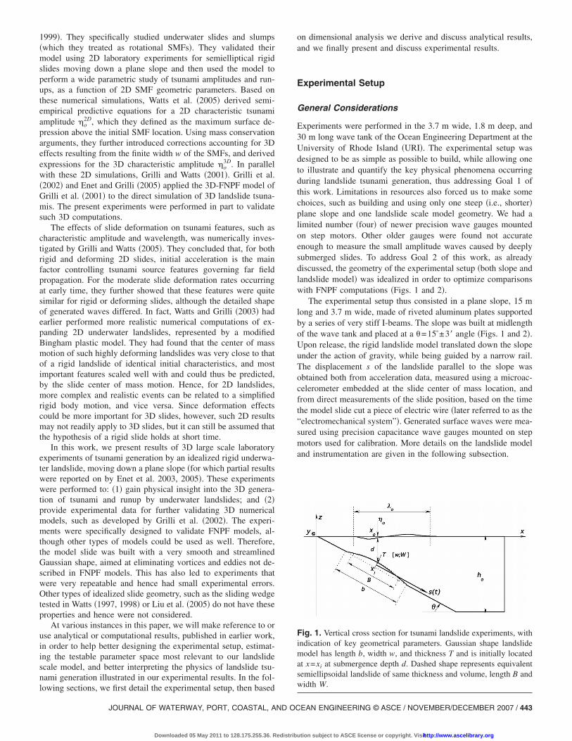
Fig. 1. Vertical cross section for tsunami landslide experiments, withindication of key geometrical parameters. Gaussian shape landslidemodel has length b, width w, and thickness T and is initially locatedat x=xi at submergence depth d. Dashed shape represents equivalentsemiellipsoidal landslide of same thickness and volume, length B andwidth W.

EAN ENGINEERING © ASCE / NOVEMBER/DECEMBER 2007 / 443


Landslide Model

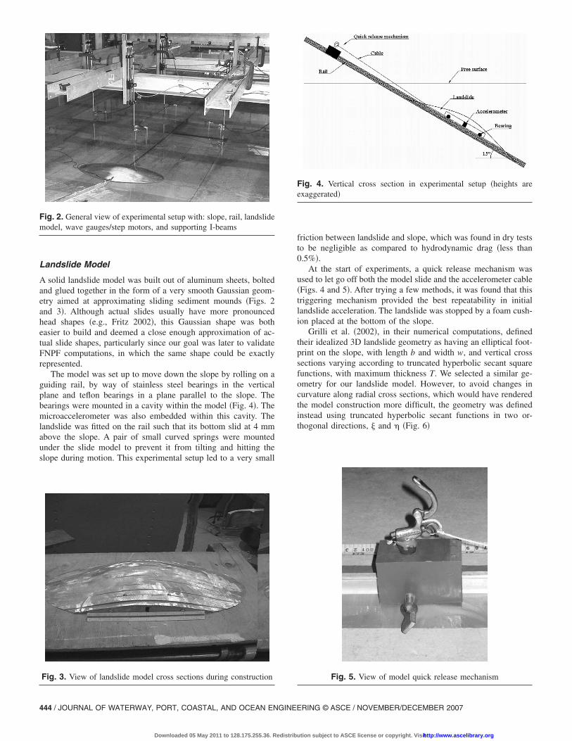
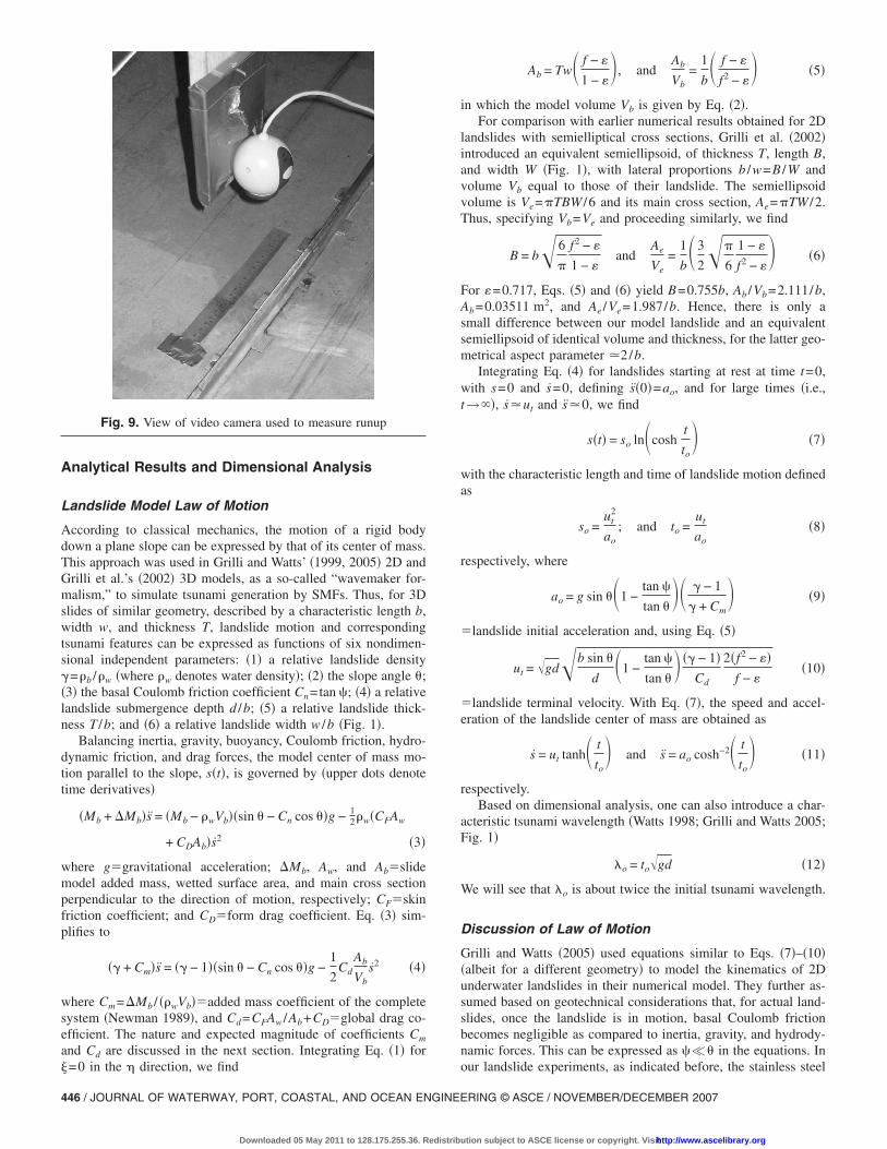
A solid landslide model was built out of aluminum sheets, boltedand glued together in the form of a very smooth Gaussian geom-etry aimed at approximating sliding sediment mounds �Figs. 2and 3�. Although actual slides usually have more pronouncedhead shapes �e.g., Fritz 2002�, this Gaussian shape was botheasier to build and deemed a close enough approximation of ac-tual slide shapes, particularly since our goal was later to validateFNPF computations, in which the same shape could be exactlyrepresented.

The model was set up to move down the slope by rolling on aguiding rail, by way of stainless steel bearings in the verticalplane and teflon bearings in a plane parallel to the slope. Thebearings were mounted in a cavity within the model �Fig. 4�. Themicroaccelerometer was also embedded within this cavity. Thelandslide was fitted on the rail such that its bottom slid at 4 mmabove the slope. A pair of small curved springs were mountedunder the slide model to prevent it from tilting and hitting theslope during motion. This experimental setup led to a very small

Fig. 2. General view of experimental setup with: slope, rail, landslidemodel, wave gauges/step motors, and supporting I-beams

Fig. 3. View of landslide model cross sections during construction



friction between landslide and slope, which was found in dry teststo be negligible as compared to hydrodynamic drag �less than0.5%�.

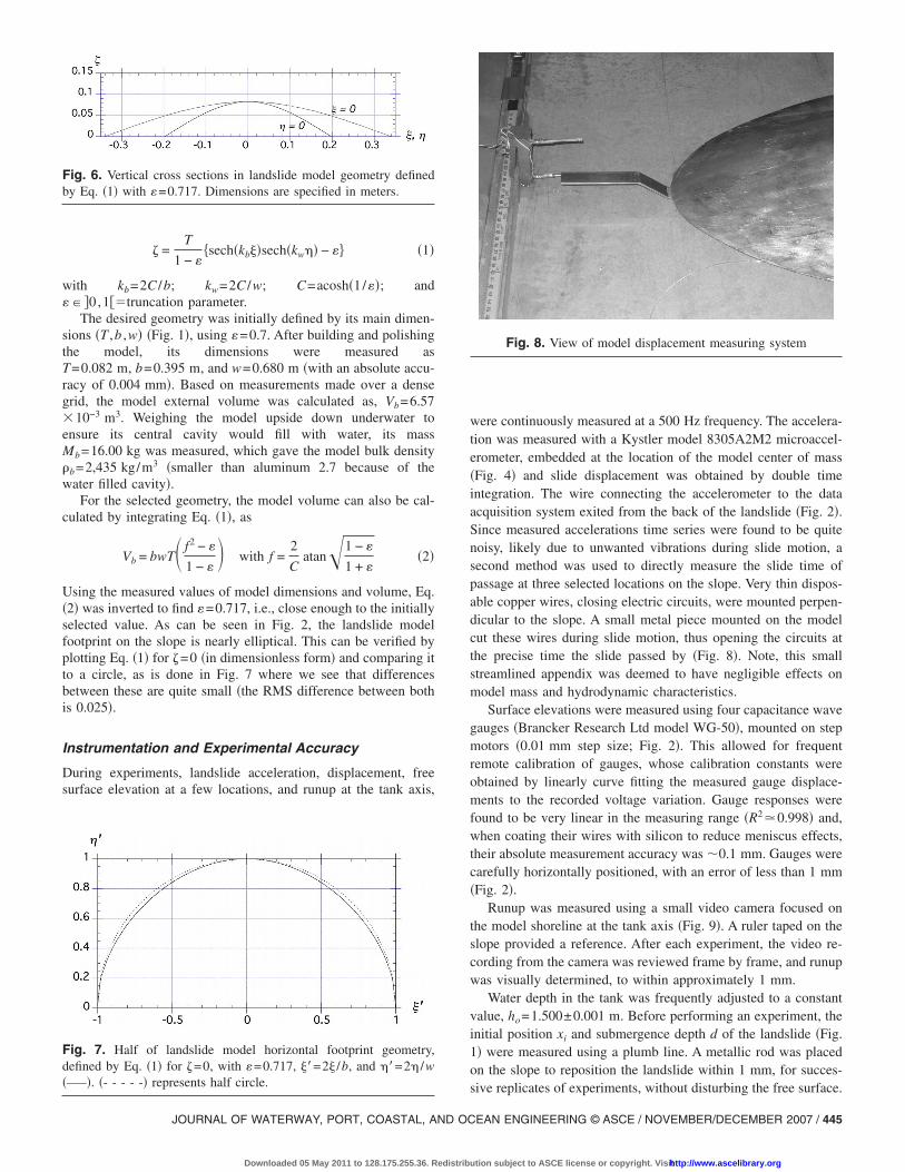
At the start of experiments, a quick release mechanism wasused to let go off both the model slide and the accelerometer cable�Figs. 4 and 5�. After trying a few methods, it was found that thistriggering mechanism provided the best repeatability in initiallandslide acceleration. The landslide was stopped by a foam cush-ion placed at the bottom of the slope.

Grilli et al. �2002�, in their numerical computations, definedtheir idealized 3D landslide geometry as having an elliptical foot-print on the slope, with length b and width w, and vertical crosssections varying according to truncated hyperbolic secant squarefunctions, with maximum thickness T. We selected a similar ge-ometry for our landslide model. However, to avoid changes incurvature along radial cross sections, which would have renderedthe model construction more difficult, the geometry was definedinstead using truncated hyperbolic secant functions in two or-thogonal directions, � and � �Fig. 6�

Fig. 4. Vertical cross section in experimental setup �heights areexaggerated�

Fig. 5. View of model quick release mechanism



� =T

1 − ��sech�kb��sech�kw�� − �� 1�

with kb=2C /b; kw=2C /w; C=acosh�1/��; and�� 0,1��truncation parameter.

The desired geometry was initially defined by its main dimen-sions �T ,b ,w� �Fig. 1�, using �=0.7. After building and polishingthe model, its dimensions were measured asT=0.082 m, b=0.395 m, and w=0.680 m �with an absolute accu-racy of 0.004 mm�. Based on measurements made over a densegrid, the model external volume was calculated as, Vb=6.57�10−3 m3. Weighing the model upside down underwater toensure its central cavity would fill with water, its massMb=16.00 kg was measured, which gave the model bulk density�b=2,435 kg/m3 �smaller than aluminum 2.7 because of thewater filled cavity�.

For the selected geometry, the model volume can also be cal-culated by integrating Eq. �1�, as

Vb = bwT� f2 − �

1 − � with f =

2

Catan1 − �

1 + ��2�

Using the measured values of model dimensions and volume, Eq.�2� was inverted to find �=0.717, i.e., close enough to the initiallyselected value. As can be seen in Fig. 2, the landslide modelfootprint on the slope is nearly elliptical. This can be verified byplotting Eq. �1� for �=0 �in dimensionless form� and comparing itto a circle, as is done in Fig. 7 where we see that differencesbetween these are quite small �the RMS difference between bothis 0.025�.

Instrumentation and Experimental Accuracy

During experiments, landslide acceleration, displacement, freesurface elevation at a few locations, and runup at the tank axis,

Fig. 6. Vertical cross sections in landslide model geometry definedby Eq. �1� with �=0.717. Dimensions are specified in meters.

Fig. 7. Half of landslide model horizontal footprint geometry,defined by Eq. �1� for �=0, with �=0.717, ��=2� /b, and ��=2� /w�—–�. �- - - - -� represents half circle.



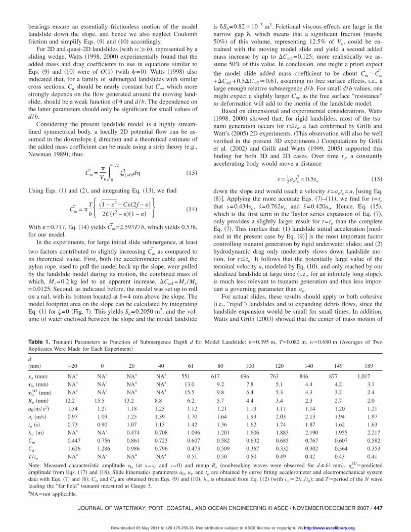
were continuously measured at a 500 Hz frequency. The accelera-tion was measured with a Kystler model 8305A2M2 microaccel-erometer, embedded at the location of the model center of mass�Fig. 4� and slide displacement was obtained by double timeintegration. The wire connecting the accelerometer to the dataacquisition system exited from the back of the landslide �Fig. 2�.Since measured accelerations time series were found to be quitenoisy, likely due to unwanted vibrations during slide motion, asecond method was used to directly measure the slide time ofpassage at three selected locations on the slope. Very thin dispos-able copper wires, closing electric circuits, were mounted perpen-dicular to the slope. A small metal piece mounted on the modelcut these wires during slide motion, thus opening the circuits atthe precise time the slide passed by �Fig. 8�. Note, this smallstreamlined appendix was deemed to have negligible effects onmodel mass and hydrodynamic characteristics.

Surface elevations were measured using four capacitance wavegauges �Brancker Research Ltd model WG-50�, mounted on stepmotors �0.01 mm step size; Fig. 2�. This allowed for frequentremote calibration of gauges, whose calibration constants wereobtained by linearly curve fitting the measured gauge displace-ments to the recorded voltage variation. Gauge responses werefound to be very linear in the measuring range �R2�0.998� and,when coating their wires with silicon to reduce meniscus effects,their absolute measurement accuracy was �0.1 mm. Gauges werecarefully horizontally positioned, with an error of less than 1 mm�Fig. 2�.

Runup was measured using a small video camera focused onthe model shoreline at the tank axis �Fig. 9�. A ruler taped on theslope provided a reference. After each experiment, the video re-cording from the camera was reviewed frame by frame, and runupwas visually determined, to within approximately 1 mm.

Water depth in the tank was frequently adjusted to a constantvalue, ho=1.500±0.001 m. Before performing an experiment, theinitial position xi and submergence depth d of the landslide �Fig.1� were measured using a plumb line. A metallic rod was placedon the slope to reposition the landslide within 1 mm, for succes-

Fig. 8. View of model displacement measuring system

sive replicates of experiments, without disturbing the free surface.



Analytical Results and Dimensional Analysis

Landslide Model Law of Motion

According to classical mechanics, the motion of a rigid bodydown a plane slope can be expressed by that of its center of mass.This approach was used in Grilli and Watts’ �1999, 2005� 2D andGrilli et al.’s �2002� 3D models, as a so-called “wavemaker for-malism,” to simulate tsunami generation by SMFs. Thus, for 3Dslides of similar geometry, described by a characteristic length b,width w, and thickness T, landslide motion and correspondingtsunami features can be expressed as functions of six nondimen-sional independent parameters: �1� a relative landslide density=�b /�w �where �w denotes water density�; �2� the slope angle �;�3� the basal Coulomb friction coefficient Cn=tan ; �4� a relativelandslide submergence depth d /b; �5� a relative landslide thick-ness T /b; and �6� a relative landslide width w /b �Fig. 1�.

Balancing inertia, gravity, buoyancy, Coulomb friction, hydro-dynamic friction, and drag forces, the model center of mass mo-tion parallel to the slope, s�t�, is governed by �upper dots denotetime derivatives�

�Mb + �Mb�s = �Mb − �wVb��sin � − Cn cos ��g − 12�w�CFAw

+ CDAb�s2 �3�

where g�gravitational acceleration; �Mb, Aw, and Ab�slidemodel added mass, wetted surface area, and main cross sectionperpendicular to the direction of motion, respectively; CF�skinfriction coefficient; and CD�form drag coefficient. Eq. �3� sim-plifies to

� + Cm�s = � − 1��sin � − Cn cos ��g −1

2Cd

Ab

Vbs2 �4�

where Cm=�Mb / ��wVb��added mass coefficient of the completesystem �Newman 1989�, and Cd=CFAw /Ab+CD�global drag co-efficient. The nature and expected magnitude of coefficients Cm

and Cd are discussed in the next section. Integrating Eq. �1� for

Fig. 9. View of video camera used to measure runup

�=0 in the � direction, we find



Ab = Tw� f − �

1 − �, and

Ab

Vb=

1

b� f − �

f2 − � �5�

in which the model volume Vb is given by Eq. �2�.For comparison with earlier numerical results obtained for 2D

landslides with semielliptical cross sections, Grilli et al. �2002�introduced an equivalent semiellipsoid, of thickness T, length B,and width W �Fig. 1�, with lateral proportions b /w=B /W andvolume Vb equal to those of their landslide. The semiellipsoidvolume is Ve=�TBW /6 and its main cross section, Ae=�TW /2.Thus, specifying Vb=Ve and proceeding similarly, we find

B = b 6

�

f2 − �

1 − �and

Ae

Ve=

1

b�3

2�

6

1 − �

f2 − � �6�

For �=0.717, Eqs. �5� and �6� yield B=0.755b, Ab /Vb=2.111/b,Ab=0.03511 m2, and Ae /Ve=1.987/b. Hence, there is only asmall difference between our model landslide and an equivalentsemiellipsoid of identical volume and thickness, for the latter geo-metrical aspect parameter �2/b.

Integrating Eq. �4� for landslides starting at rest at time t=0,with s=0 and s=0, defining s�0�=ao, and for large times �i.e.,t→ �, s�ut and s�0, we find

s�t� = so ln�cosht

to �7�

with the characteristic length and time of landslide motion definedas

so =ut

2

ao; and to =

ut

ao�8�

respectively, where

ao = g sin ��1 −tan

tan �� − 1

+ Cm �9�

�landslide initial acceleration and, using Eq. �5�

ut = gdb sin �

d�1 −

tan

tan � � − 1�

Cd

2�f2 − ��f − �

�10�

�landslide terminal velocity. With Eq. �7�, the speed and accel-eration of the landslide center of mass are obtained as

s = ut tanh� t

to and s = ao cosh−2� t

to �11�

respectively.Based on dimensional analysis, one can also introduce a char-

acteristic tsunami wavelength �Watts 1998; Grilli and Watts 2005;Fig. 1�

�o = togd �12�

We will see that �o is about twice the initial tsunami wavelength.

Discussion of Law of Motion

Grilli and Watts �2005� used equations similar to Eqs. �7�–�10��albeit for a different geometry� to model the kinematics of 2Dunderwater landslides in their numerical model. They further as-sumed based on geotechnical considerations that, for actual land-slides, once the landslide is in motion, basal Coulomb frictionbecomes negligible as compared to inertia, gravity, and hydrody-namic forces. This can be expressed as �� in the equations. In
our landslide experiments, as indicated before, the stainless steel


bearings ensure an essentially frictionless motion of the modellandslide down the slope, and hence we also neglect Coulombfriction and simplify Eqs. �9� and �10� accordingly.

For 2D and quasi-2D landslides �with w�b�, represented by asliding wedge, Watts �1998, 2000� experimentally found that theadded mass and drag coefficients to use in equations similar toEqs. �9� and �10� were of O�1� �with =0�. Watts �1998� alsoindicated that, for a family of submerged landslides with similarcross sections, Cd should be nearly constant but Cm, which morestrongly depends on the flow generated around the moving land-slide, should be a weak function of � and d /b. The dependence onthe latter parameters should only be significant for small values ofd /b.

Considering the present landslide model is a highly stream-lined symmetrical body, a locally 2D potential flow can be as-sumed in the downslope � direction and a theoretical estimate ofthe added mass coefficient can be made using a strip theory �e.g.,Newman 1989�; thus

Cm =�

Vb�

0

w/2

��=0�2 d� �13�

Using Eqs. �1� and �2�, and integrating Eq. �13�, we find

Cm = �T

b 1 − �2 − C��2f − ��

2C�f2 − ��1 − �� 14�

With �=0.717, Eq. �14� yields Cm=2.593T /b, which yields 0.538,for our model.

In the experiments, for large initial slide submergence, at least

two factors contributed to slightly increasing Cm as compared toits theoretical value. First, both the accelerometer cable and thenylon rope, used to pull the model back up the slope, were pulledby the landslide model during its motion, the combined mass ofwhich, Mr=0.2 kg led to an apparent increase, �Cm1=Mr /Mb

=0.0125. Second, as indicated before, the model was set up to rollon a rail, with its bottom located at �=4 mm above the slope. Themodel footprint area on the slope can be calculated by integratingEq. �1� for �=0 �Fig. 7�. This yields Sb=0.2050 m2, and the vol-ume of water enclosed between the slope and the model landslide

Table 1. Tsunami Parameters as Function of Submergence Depth d foReplicates Were Made for Each Experiment�

d�mm� −20 0 20 40 61

xo �mm� NAa NAa NAa NAa 551

�o �mm� NAa NAa NAa NAa 13.0

�o3D �mm� NAa NAa NAa NAa 15.5

Ru �mm� 12.2 15.5 13.2 8.8 6.2

a0�m/s2� 1.34 1.21 1.18 1.23 1.12

ut �m/s� 0.97 1.09 1.25 1.39 1.70

to �s� 0.73 0.90 1.07 1.13 1.42

�o �m� NAa NAa 0.474 0.708 1.096

Cm 0.447 0.756 0.861 0.723 0.607

Cd 1.626 1.286 0.986 0.796 0.473

T / to NAa NAa NAa NAa 0.51

Note: Measured characteristic amplitude �o �at x=xo and y=0� and ruamplitude from Eqs. �17� and �18�. Slide kinematics parameters a0, ut, adata with Eqs. �7� and �8�; Cm and Cd are obtained from Eqs. �9� and �10leading the “far field” tsunami measured at Gauge 3.a
NA�not applicable.


is �Sb=0.82�10−3 m3. Frictional viscous effects are large in thenarrow gap �, which means that a significant fraction �maybe50%� of this volume, representing 12.5% of Vb, could be en-trained with the moving model slide and yield a second addedmass increase by up to �Cm2=0.125; more realistically we as-sume 50% of this value. In conclusion, one might a priori expect

the model slide added mass coefficient to be about Cm�Cm

+�Cm1+0.5�Cm2�0.61, assuming no free surface effects, i.e., alarge enough relative submergence d /b. For small d /b values, onemight expect a slightly larger Cm, as the free surface “resistance”to deformation will add to the inertia of the landslide model.

Based on dimensional and experimental considerations, Watts�1998, 2000� showed that, for rigid landslides, most of the tsu-nami generation occurs for t� to, a fact confirmed by Grilli andWatt’s �2005� 2D experiments. �This observation will also be wellverified in the present 3D experiments.� Computations by Grilliet al. �2002� and Grilli and Watts �1999, 2005� supported thisfinding for both 3D and 2D cases. Over time to, a constantlyaccelerating body would move a distance

s = 12aoto

2 = 0.5so �15�

down the slope and would reach a velocity s=aoto=ut �using Eq.�8��. Applying the more accurate Eqs. �7�–�11�, we find for t= to

that s=0.434so, s=0.762ut, and s=0.420ao. Hence, Eq. �15�,which is the first term in the Taylor series expansion of Eq. �7�,only provides a slightly larger result for t= to than the completeEq. �7�. This implies that: �1� landslide initial acceleration �mod-eled in the present case by Eq. �9�� is the most important factorcontrolling tsunami generation by rigid underwater slides; and �2�hydrodynamic drag only moderately slows down landslide mo-tion, for t� to. It follows that the potentially large value of theterminal velocity ut modeled by Eq. �10�, and only reached by ouridealized landslide at large time �i.e., for an infinitely long slope�,is much less relevant to tsunami generation and thus less impor-tant a governing parameter than ao.

For actual slides, these results should apply to both cohesive�i.e., “rigid”� landslides and to expanding debris flows, since thelandslide expansion would be small for small times. In addition,Watts and Grilli �2003� showed that the center of mass motion of

el Landslide: b=0.395 m, T=0.082 m, w=0.680 m �Averages of Two

80 100 120 140 149 189

17 696 763 846 877 1,017

9.2 7.8 5.1 4.4 4.2 3.1

9.8 6.4 5.3 4.3 3.2 2.4

5.7 4.4 3.4 2.3 2.7 2.0

1.21 1.19 1.17 1.14 1.20 1.21

1.64 1.93 2.03 2.13 1.94 1.97

1.36 1.62 1.74 1.87 1.62 1.63

1.201 1.606 1.883 2.190 1.955 2.217

0.582 0.632 0.685 0.767 0.607 0.582

0.509 0.367 0.332 0.302 0.364 0.353

0.50 0.50 0.49 0.42 0.43 0.41

u �nonbreaking waves were observed for d�61 mm�. �o3D�predicted

re obtained by curve fitting accelerometer and electromechanical systemobtained from Eq. �12� �with co�2�o / to�; and T�period of the N wave

r Mod

6

nup Rnd to a�; �o is



expanding landslides described by a modified Bingham plasticmodel is still well represented by an equation of the type Eq. �7�.Finally, the plane slope approximation should also hold for morecomplex bottom topographies, when assuming small times andthus small slide displacements.

The expected magnitude of the global drag coefficient Cd alsodeserves some attention. For small T /b values, the skin frictioncoefficient can be estimated to be that of a flat plate in a turbulentflow �Newman 1989�

CF =0.0986

�log R − 1.22�2 �16�

with R=Ub /��flow Reynolds number; U�reference flow veloc-ity; and ��kinematic viscosity, about 10−6 m2/s for water. Forsmall T /b values, U near the landslide model should be close atall times to the model center of mass velocity, given by Eq. �11�,reaching a maximum of ut for large time. Assuming, for simplic-ity, that the water velocity near the landslide model surface isaround ut /2 on average, and noting that we will find ut�2 m/sin these experiments �Table 1�, we estimate R�4�105, andCF�0.00514. Now, the model wetted surface area Aw is slightlymore than 2Sb=0.41 m2. Hence, CFAw /Ab�0.06. Finally, for thisslender body in a turbulent flow �large R�O�105� value�, theform drag coefficient can be expected to be about CD=0.3 �theaverage value for ellipses of aspect ratio 2:1 to 4:1�. Therefore,we find an expected minimum value of the global drag coeffi-cient, Cd�0.36.

Dispersive and Nonlinear Effects in GeneratedTsunamis

In designing these laboratory experiments, we found it desirableto a priori estimate the magnitude of dispersive and nonlineareffects in the generated tsunamis, and verify that the tested pa-rameter space would make it possible for these effects to show upin experimental results.

Making the usual nondimensional arguments for gravitywaves, one can express dispersive effects in SMF tsunamis by arelative depth parameter, �=d /�o. Assuming linear periodicwaves in constant depth, a value of � greater than �0.5 indicatesfully dispersive deep water waves, whereas a value of � less than�0.05 indicates nondispersive long waves �e.g., Dean and Dal-rymple 1991�. Nonlinear effects in periodic gravity waves can besimilarly expressed by a steepness parameter �=a /�o, where adenotes wave amplitude. In general, the smaller the value of �, themore applicable linear wave theory. Specifically, Le Mehauté�1976� proposed a limit for the applicability of linear wave theoryin deep water: ��0.0031, with a gradual reduction of this valuein intermediate water depth, as depth decreases, down to��0.00017 for the shallow water depth limit. At the other end ofthe range of variation of �, we find an upper bound, i.e., a maxi-mum wave nonlinearity, corresponding to the breaking limit. Fordeep water waves, Miche’s criterion yields ��0.07, a value thatis also usually assumed to decrease as a function of depth, accord-ing to a variety of empirical criteria, the simplest of which being,for very mild slopes, 2a /d�0.78 or ��0.39�, which corre-sponds to the maximum stable solitary wave �see, e.g., Dean andDalrymple 1991�.

Watts et al. �2005� gave an estimate of the characteristic am-plitude �o of tsunamis caused by 3D rigid landslides, defined asthe maximum depression above the landslide initial location ofminimum submergence depth d �Fig. 1�. This estimate applied to
landslides with equivalent semiellipsoid dimensions �B ,T ,W� and


was based on semiempirical equations derived from many resultsof 2D fully nonlinear potential flow computations �Grilli andWatts 1999, 2005�, with an ad hoc 3D correction. The character-istic amplitude scaled with so and was expressed as a function offive nondimensional parameters, as

�o3D = soF��G��T

B�B sin �

d1.25� 1

1 + �o/w �17�

with the empirical functions

F = 0.0486 − 0.0302 sin � and G = 1.18�1 − e−2.2�−1��

�18�

and ��30°, T /B�0.2, 1.46��2.93, and d /B�0.06. In Eq.�17�, 3D amplitudes �o

3D were simply obtained from the calcu-lated 2D amplitudes �o

2D by invoking mass conservation, whichled to the last term, the function of �o /w.

Following the same procedure that led to Eqs. �4�–�12�, dis-persion and nonlinearity parameters �� ,�� can therefore be esti-mated for 3D landslide tsunamis as �with =0�

� =d

�o=d sin �

B � + Cm� �

2Cd� − 1��−1

�19�

and

� =�o

3D

�o= �T

B�B sin �

d1.75� 1

1 + �o/w F��G�� − 1�

2Cd�

�20�

in which Ab /Vb=4/ ��B� was used, based on the quasi-2D semiel-liptical landslides computations from which Eq. �17� was derived.

Eqs. �19� and �20� yield: �� d /B�0.5 and �� d /B�−1.75 for ourexperiments, which were performed over a single plane slope��=15° �, with a single landslide density �=2.44�, and for asingle relative landslide width �w /b=W /B=1.72� and thickness�T /b=0.21, T /B=0.27�. This implies that, with a single landslidemodel, one can only simultaneously but not independently vary �and � by varying the initial submergence depth d in experiments.To vary both dispersion and nonlinearity parameters indepen-dently, one would have to use at least two landslide models withdifferent T /B values, assuming the same density is used. Morespecifically, for our model, Eq. �6� yields the equivalent ellipsoiddimensions: T=0.082 m, B=0.298 m, and W=0.513 m. Based onthe above discussion, assuming Cm�0.61 and Cd�0.36 for lackof more accurate values at this stage, Eqs. �18� yields F=0.0408and G=1.130, and Eq. �19�, �=0.0958�d /B�0.5.

Assuming w��o to start with, i.e., quasi-2D results, Eq. �20�yields �=2.27�10−3�d /B�−1.75. In this result, T /B is slightly toolarge for Eq. �17� to strictly apply, and w /b=1.72 is quite smalland hence one should expect—and we will actually observe—significant 3D tsunami generation effects in our experiments. Eq.�12� gives an estimate of �o, proportional to to, itself given byEqs. �8�–�10�. For the approximate values of Cm and Cd, we thusfind ao=1.20 m/s2, ut=1.95 m/s, to=1.63 s, and �o=5.09d.

For the submergence depths d=61–189 mm that will prima-rily be tested in our experiments �Table 1�, we find an average 3Damplitude correction in Eqs. �17� and �20�: �o

3D /�o2D=1/ �1

+�o /w��0.286, which reduces the nonlinearity parameter to,�=6.49�10−4 �d /B�−1.75 and finally yields: �=1.77 10−7 �−3.5.This equation is plotted in Fig. 10, in the �� ,�� nonlinearity-dispersion space, together with the limit for linear wave theory
and the breaking criterion discussed above.


Watts �1998, 2000� used parameter b sin � /d to express non-linear effects in generated SMF tsunamis. Based on Eq. �20�, thisparameter reads ��1+�o /w� /0.0312�1/1.75 for our model. Assum-ing the maximum nonlinearity value �=0.39d /�o from the break-ing criterion, we find a maximum for b sin � /d=4.23�d�1/�o

+1/w��0.571. For our model slide geometry and using Eq. �12�,this leads to a submergence depth d=65 mm, below which wavebreaking should occur in the experiments. We have �=0.044 forthis depth, indicating initially shallow water tsunami waves �Fig.10�, and b sin � /d=1.57, implying a strongly nonlinear tsunami�Watts 2000�. In the experiments we found by successive trialsthat, for d�61 mm, tsunami waves started breaking above thesubmerged body, which is quite close to the above predicteddepth threshold. We thus selected d=61 mm as the minimum sub-mergence depth tested for nonbreaking waves.

Finally, for linear wave theory to apply, the selected criterionyields �Fig. 10�, ��0.0066�−0.00016, and we find b sin � /d�0.321, or d�318 mm �for which �=0.098�. Therefore, withour model slide, to fully explore nonlinear effects for nonbreakinglandslide tsunami generation, we should test submergence depthsfrom d�61 to 318 mm. Within this depth range, generated waveswould be mostly dispersive intermediate water depth waves.

Experimental Results

As discussed above, in these experiments, we only tested thedependence of tsunami features on submergence depth d /b, for asingle model slide and one slope angle. Seven submergencedepths were tested in between d=61 mm, representing theobserved breaking limit, and d=189 mm, the selected deepestsubmergence �for which tsunami characteristic amplitude wasonly about 3 mm; Table 1�. For larger submergence depths, gen-erated waves were too small for making accurate and repeatablemeasurements. An additional four experiments were performedfor depths in between d=−20 mm �i.e., for the slide being partlyemerged� and d=61 mm. Tested submergence depths were spacedevenly in this interval, every 20 mm or so, except ford=149 mm, due to difficulties in positioning wave gauges�Table 1�.

Each experiment was repeated once. As we will see, becauseof the very small differences between replicates, these were aver-aged to reduce experimental errors. Data processing is discussed

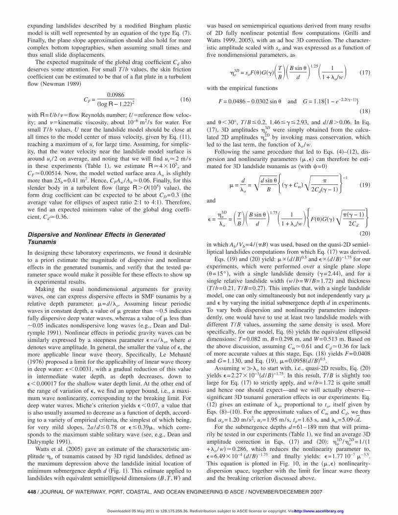
Fig. 10. Estimated testable parameters in tsunami landslideexperiments: �� actual values tested in experiments �with �o

estimated with Eq. �12��: �BC� breaking criterion; �LWT� linear wavetheory; �SW� shallow water waves; �IW� intermediate water depthwaves

below. For d�61 mm, gauge 1 was always located above the



landslide point of minimum submergence, at x=xo=d / tan �+T / sin � and y=0 �see Table 1�, to measure ��xo , t� �Fig. 1�, fromwhich the characteristic tsunami amplitude is obtained as�o=MAX ��xo , t��. For d�61 mm, there was not enough spaceto locate a gauge at xo. In all tests, the other three gauges werekept at fixed locations �x ,y��Gauge 2 �1,469, 350�; Gauge 3�1,929, 0�; Gauge 4 �1,929,500� mm. �Note, Gauges 2 and 3 wereinitially located symmetrically about the tank axis and, after veri-fying that all generated waves were symmetrical, these gaugeswere relocated at their final location listed above. Also note thatGauges 3 and 4 are located at the same x value and almost thesame radial distance, 1,929 and 1,992 mm, from the origin ofaxes.� Runup Ru �i.e., maximum vertical water elevation frommean water level on the slope� was measured at the tank axis�y=0� for each tested depth.

Experimental results are summarized in Table 1, and analyzedand discussed in the following subsection.

Landslide Kinematics

In each experiment, the microaccelerometer recorded the land-slide center of mass acceleration parallel to the slope as a functionof time s�t�, and the electromechanical system measured the timeof passage of the slide t�sgk� �k=1,2 ,3�, at three gate locations

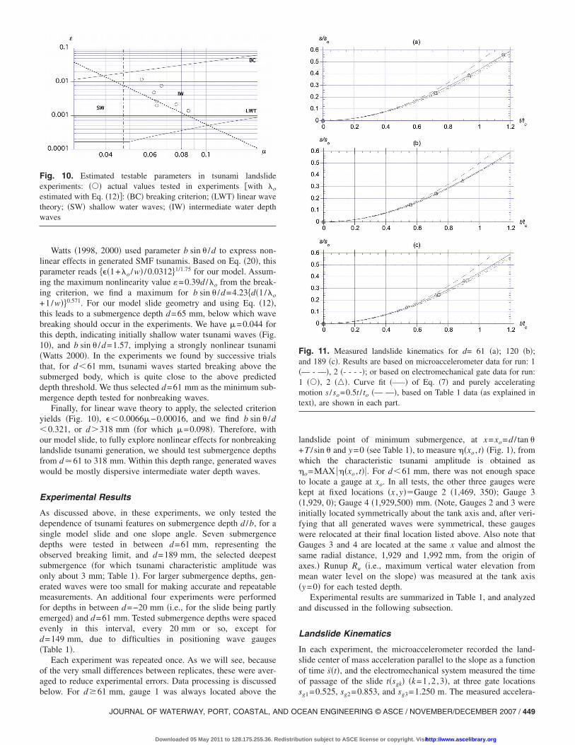
Fig. 11. Measured landslide kinematics for d= 61 �a�; 120 �b�;and 189 �c�. Results are based on microaccelerometer data for run: 1�— - —�, 2 �- - - -�; or based on electromechanical gate data for run:1 ��, 2 ��. Curve fit �—–� of Eq. �7� and purely acceleratingmotion s /so=0.5t / to �— —�, based on Table 1 data �as explained intext�, are shown in each part.

sg1=0.525, sg2=0.853, and sg3=1.250 m. The measured accelera-



tion was twice time integrated to provide slide center of massmotion. Fig. 11 shows examples of slide center of mass motionobtained from both acceleration and gate data, for two replicatesof experiments performed for d=61, 120, and 189 mm. Theseresults first show that experiments are well repeatable and, sec-ond, that slide motions independently obtained from the gates andthe microaccelerometer data are in good agreement with eachother.

Slide motions s�t� derived from either the gate or accelerationdata were used to curve fit the theoretical law of motion given byEqs. �7� and �8�, for each experiment; this yielded the slide initialacceleration ao and terminal velocity ut for each case. When com-paring these curve fitted parameters to the raw data, it was foundthat the measured initial acceleration �obtained from a linearcurve fit of data over a very small time, �0.1 s� was a morerepeatable value between replicates than parameter ao derivedfrom the curve fitted slide motions �whether from the gate oracceleration data�. Measured accelerations, however, becamequite noisy for larger times �on the order of t�0.5to�, likely dueto shocks and vibrations occurring during slide motion, yieldingincreased uncertainty for integrated slide motions and ut derivedfrom these through curve fitting. On the other hand, the time ofpassage at gates provided a more repeatable estimate of ut �alsothrough curve fitting of Eqs. �7� and �8��. Hence, for each experi-ment, we combined the gate and acceleration data �averaged overtwo replicates�, by using the ao value derived from small timeacceleration data and calculating the ut value as the only param-eter derived from gate data, by curve fitting Eqs. �7� and �8�.Results of this combined method are given in Table 1 for all thetests. Curve fitted slide motions for the three depths mentionedabove are shown in Fig. 11, on which we clearly see that thecurve fits closely match the data derived from accelerations atsmall times but fit the gate data better at larger times.

With these results for ao and ut, we calculate values of to inTable 1 using Eq. �8�, and of �o using Eq. �12�. We see that to

gradually increases from d=−20 to 140 mm and fits a linear equa-tion, to�0.900+7.07d quite well �R2=0.974, d in meters�. Thetwo deepest submergence depths, however, do not follow thistrend as ut tends to level up maybe because of the influence ofshocks that occur in deeper water at the joint between two alumi-num plates in the model slope. The estimated characteristic tsu-nami wavelength follows the same trend as to, increasing fromd=−20 to 140 mm and then stabilizing. Using this estimate andthe measured values of �o, one can calculate the locations ofnonbreaking experimental tests �d�61 mm� in the �� ,�� space.These are plotted in Fig. 10 where we see that experiments dis-tribute about the theoretical relationship derived earlier and allcorrespond to dispersive intermediate water depth waves.

Eqs. �9� and �10� finally yield the Cm and Cd values for theexperimental data in Table 1 �with f =0.8952 for our model�. Theadded mass coefficients Cm, expectedly, increase when d variesfrom partial slide emergence to shallow submergence, and thendecrease to reach an average value of 0.637 for d�61 mm, whichis in good agreement with our theoretical estimate of 0.61. Valuesof Cd decrease from emergence to shallow submergence, to reachan average of 0.386 for d�61, which is also in good agreementwith our theoretical estimate of 0.36.

Finally, as also noted in earlier work �e.g., Watts 1998, 2000;Grilli and Watts 2005�, Fig. 11 shows that, for t�0.5to, slidekinematics can essentially be modeled by s=aot2 /2 or s /so

=0.5t / to, i.e., as a purely accelerating body that viscous drag
forces have not yet significantly slowed down. Hence, the small


shocks observed in experiments for later times, which affect thevalue of ut, do not greatly affect slide kinematics at early times.

Free Surface Elevations

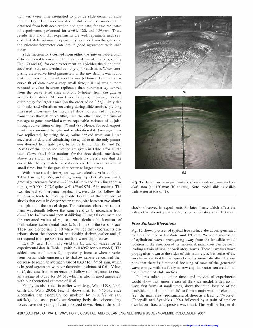
Fig. 12 shows pictures of typical free surface elevations generatedby the slide motion for d=61 and 120 mm. We see a successionof cylindrical waves propagating away from the landslide initiallocation in the direction of its motion. A main crest can be seen,leading a train of smaller oscillatory waves. There is weaker wavepropagation towards the sides of this main crest, but some of thesmaller waves that follow spread slightly more laterally. This im-plies that there is directional focusing of most of the generatedwave energy, within a fairly narrow angular sector centered aboutthe direction of slide motion.

Pictures taken at earlier times and movies of experimentswould show that, upon release of the slide model, a depressionwave first forms at small times, above the initial location of thelandslide, and then “rebounds” to form a main wave of elevation�i.e., the main crest� propagating offshore as a leading “N-wave”�Tadepalli and Synolakis 1994� followed by a train of smaller

Fig. 12. Examples of experimental surface elevations generated ford=61 mm �a�; 120 mm; �b� at t� to. Note, model slide is visibleunderwater at top of �b�.

oscillations �i.e., a dispersive wave tail�. This will be further il-



lustrated below based on measured surface elevations at gauges.The “rebound” wave also propagates shoreward and reflects onthe slope, causing runup and some of the smaller waves seen, forinstance, at the bottom of Fig. 12�b�.

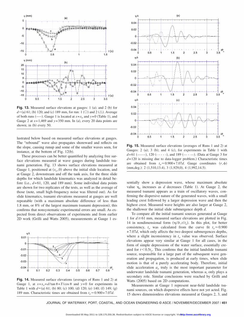
These processes can be better quantified by analyzing free sur-face elevations measured at wave gauges during landslide tsu-nami generation. Fig. 13 shows surface elevations measured atGauge 1, positioned at �xo ,0� above the initial slide location, andat Gauge 2, downstream and off the tank axis, for the three slidedepths for which landslide kinematics was analyzed in detail be-fore �i.e., d=61, 120, and 189 mm�. Some individual data pointsare shown for two replicates of the tests, as well as the average ofthose �note, small high-frequency noise was filtered out�. As forslide kinematics, tsunami elevations measured at gauges are wellrepeatable �with a maximum absolute difference of less than1.8 mm, or 8% of the largest maximum tsunami depression�; thisconfirms that nonsystematic experimental errors are small. As ex-pected from direct observations of experiments and from earlier2D work �Grilli and Watts 2005�, measurements at Gauge 1 es-

Fig. 13. Measured surface elevations at gauges: 1 �a�; and 2 �b� ford��a� 61; �b� 120; and �c� 189 mm, for run: 1 �� and 2 ��. Averageof both runs �—–�. Gauge 1 is located at x=xo and y=0 �Table 1�, andGauge 2 at x=1,469 and y=350 mm. In �a�, every 20 data points areshown; in �b� every 50.

Fig. 14. Measured surface elevations �averages of Runs 1 and 2� atGauge 1, at x=xo=d / tan �+T / cos � and y=0 for experiments inTable 1 with d��a� 61; �b� 80; �c� 100; �d� 120; �e� 140; �f� 149; �g�189 mm. Characteristic times are obtained from to�0.900+7.07d.



sentially show a depression wave, whose maximum absolutevalue �o increases as d decreases �Table 1�. At Gauge 2, themeasured tsunami appears as a train of oscillatory waves, con-firming the dispersive nature of the generated waves, with a smallleading crest followed by a larger depression wave and then thehighest crest. Measured wave heights are also larger at Gauge 2,the shallower the initial slide submergence depth d.

To compare all the initial tsunami sources generated at Gauge1 for d�61 mm, measured surface elevations are plotted in Fig.14 in nondimensional form �� /b , t / to�. In this plot, for betterconsistency, to was calculated from the curve fit to�0.900+7.07d, which only affects the two deepest submergences depths,where a slight inconsistency in to value was observed. Surfaceelevations appear very similar at Gauge 1 for all cases, in theform of simple depressions of the water surface, essentially cre-ated for t�0.5to. This confirms that the initial landslide tsunamisource, responsible for a large part of the subsequent wave gen-eration and propagation, is produced at early times, when slidemotion is that of a purely accelerating body. Therefore, initialslide acceleration ao truly is the most important parameter forunderwater landslide tsunami generation, whereas ut only plays asecondary role. Similar conclusions were reached by Grilli andWatts �2005� based on 2D computations.

Measurements at Gauge 1 represent near-field landslide tsu-nami sources, on which dispersive effects have not yet acted. Fig.

Fig. 15. Measured surface elevations �averages of Runs 1 and 2� atGauges: 2 �a�; 3 �b�; and 4 �c�, for experiments in Table 1 withd=61 �——-�, 120 �- - - - -�, and 189 �— - —�. �Data at Gauge 3 ford=120 is missing due to data-logger problem.� Characteristic timesare obtained from to�0.900+7.07d. Gauge coordinates �r ,��mm,deg.�: 2 �1,510,13.4�, 3 �1,929,0�, 4 �1,992,14.5�.

15 shows dimensionless elevations measured at Gauges 2, 3, and



¯

4 for d=61, 120, and 189 mm, which are examples of far fieldlandslide tsunamis. In each case, the tsunami appears as a welldeveloped train of oscillatory waves, indicative of strong disper-sive effects; a large depression wave is preceded by a small lead-ing elevation wave �about four times smaller�, and followed bythe largest elevation wave in the train �slightly larger than thedepression wave�. Thus, the salient feature of these tsunamis is aso-called leading N wave. As noted before, the tsunami amplitudeis larger, the shallower the initial slide submergence. Gauges 2, 3,and 4 are located at radial distances r=1,510, 1,929, and1,992 mm, respectively, from the origin of the coordinate system.Gauges 2 and 4 have an azimuth of �=13.4 and 14.5°, respec-tively, with respect to the tank axis. Measurements at Gauge 3,which is on the tank axis, show the largest tsunamis, despite thegauge being almost the farthest from the origin. Waves are muchsmaller at the nearer Gauge 2, and at Gauge 4, which is at aboutthe same radial distance as 3 but off the axis. This is consistentwith our observations of a directional tsunami �Fig. 12�.

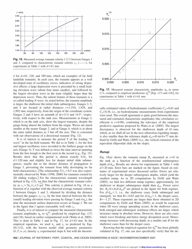
It is of interest to measure the period T of the leading “Nwave” in the far-field tsunami. We did so in Table 1, for the firstand largest oscillatory wave recorded at the farthest gauge on theaxis �Gauge 3�; T was defined as twice the time interval spanningfrom the first trough to the first crest in the record �e.g., Fig. 15�.Results show that this period is almost exactly 0.5to ford�120 mm and slightly less for deeper initial slide submer-gences, maybe due to the shorter distance of propagation toGauge 3, preventing the tsunami from fully developing its farfield characteristics. �The relationship T / to�0.5 was also experi-mentally observed by Watts �1998, 2000� for tsunamis created by2D sliding wedges.� For the characteristic tsunami wavelengthdefined in Eq. �12�, we thus find the characteristic tsunami celer-ity as co�2�o / to=2gd. This celerity is plotted in Fig. 16 as afunction of d, together with the observed average tsunami celerityc between Gauges 1 and 3, obtained by dividing the distancebetween the gauges, x3−xo, by the time interval between the first�small� leading elevation wave passing by Gauge 3 and t��o�, thetime the maximum surface depression occurs at Gauge 1. We seein the figure that c agrees reasonably well with co.

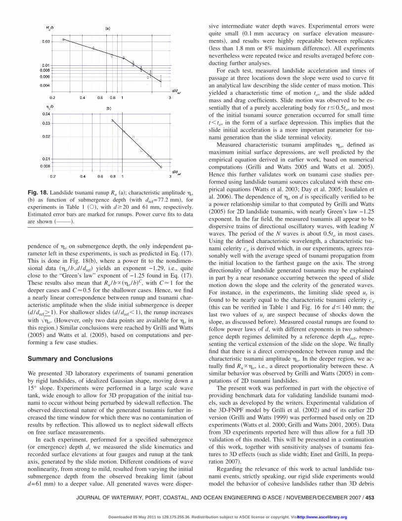
Finally, it is of interest to compare the measured characteristictsunami amplitudes �o to �o

3D, predicted by empirical Eqs. �17�and �18�, based on earlier computational work �Watts et al. 2005�.This is done in Table 1 and in Fig. 17, for d�61 mm. In theempirical equations, we used �o and so as predicted by Eqs.�8�–�12�, with the known model slide geometry parameters

Fig. 16. Measured average tsunami celerity c �� between Gauges 1and 3, compared to characteristic tsunami celerity co �——–�, forexperiments in Table 1 with d�61 mm

�b ,T ,w ,��, density , experimental slope �, but with the theoreti-



cally estimated values of hydrodynamic coefficients Cm=0.61 andCd=0.36, i.e., no hydrodynamic measurements from experimentswere used. The overall agreement is quite good between the mea-sured and estimated characteristic amplitudes �the correlation co-efficient is r=0.98�, confirming the relevance of the empiricalpredictive equations proposed by Watts et al. �2005�. The largestdiscrepancy is observed for the shallowest depth of 61 mm,which, as we shall all see in the next subsection regarding runups,is also smaller than the reference depth dref=B sin �=77 mm de-fined by Grilli and Watts �2005� �i.e., the vertical extension of theequivalent ellipsoidal slide on the slope�.

Runup

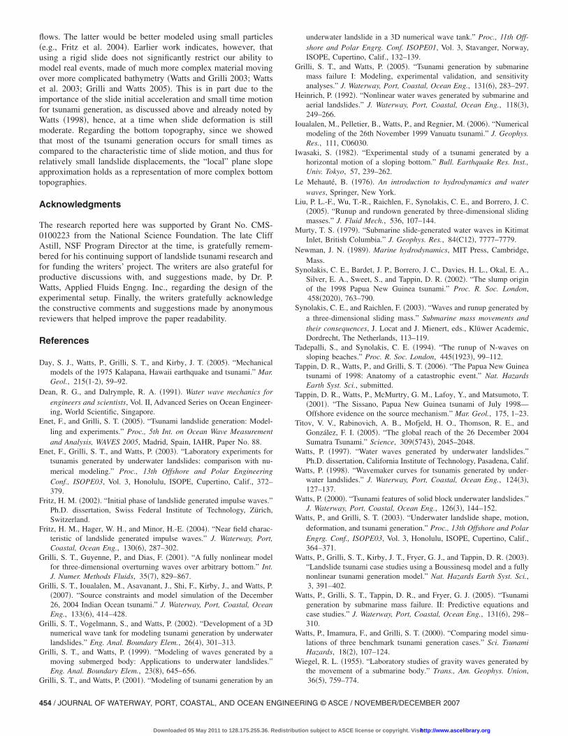
Fig. 18�a� shows the tsunami runup Ru measured at y=0 inthe tank as a function of the nondimensional submergencedepth d /dref. Results are shown for experiments in Table 1 withd�20 mm. Error bars are marked on the figure, based on esti-mates of experimental errors discussed earlier. Errors are rela-tively larger for the deeper submergence depths, which yield thesmallest runup. As in 2D computations by Grilli and Watts�2005�, we find two different runup regimes, approximately, forshallower or deeper submergence depth than dref. Power curvefits: Ru /b=A�d /dref�B are plotted in the figure for both regimes.For d /dref�1, i.e., the shallower cases �both submerged andemerged�, we find B=−0.63 and for d /dref�1, the deeper cases,B=−1.27. These exponents are larger than those obtained in 2Dcomputations by Grilli and Watts �2005�, as would be expectedwhen 3D wave energy spreading occurs. In the shallower cases,both emerged and submerged, nonlinear effects are larger, whichincreases runup in absolute terms. However, these are also caseswhere wave breaking and hence energy dissipation occur. Hence,runup increases with decreasing depth, at a smaller rate B for theshallower cases than for the deeper cases.

Knowing that the empirical equation for �o3D has been globally

Fig. 17. Measured tsunami characteristic amplitudes �o in meter��, compared to empirical predictions �o

3D �Eqs. �17� and �18��, forexperiments in Table 1 with d�61 mm

validated in Fig. 17, one can also specifically verify that the de-



pendence of �o on submergence depth, the only independent pa-rameter left in these experiments, is such as predicted in Eq. �17�.This is done in Fig. 18�b�, where a power fit to the nondimen-sional data ��o /b ,d /dref� yields an exponent −1.29, i.e., quiteclose to the “Green’s law” exponent of −1.25 found in Eq. �17�.These results also mean that Ru /b� ��o /b�C, with C�1 for thedeeper cases and C�0.5 for the shallower cases. Hence, we finda nearly linear correspondence between runup and tsunami char-acteristic amplitude when the slide initial submergence is deeper�d /dref�1�. For shallower slides �d /dref�1�, the runup increaseswith �o. �However, only two data points are available for �o inthis region.� Similar conclusions were reached by Grilli and Watts�2005� and Watts et al. �2005�, based on computations and per-forming a few case studies.

Summary and Conclusions

We presented 3D laboratory experiments of tsunami generationby rigid landslides, of idealized Gaussian shape, moving down a15° slope. Experiments were performed in a large scale wavetank, wide enough to allow for 3D propagation of the initial tsu-nami to occur without being perturbed by sidewall reflection. Theobserved directional nature of the generated tsunamis further in-creased the time window for which there was no contamination ofresults by reflection. This allowed us to neglect sidewall effectson free surface measurements.

In each experiment, performed for a specified submergence�or emergence� depth d, we measured the slide kinematics andrecorded surface elevations at four gauges and runup at the tankaxis, generated by the slide motion. Different conditions of wavenonlinearity, from strong to mild, resulted from varying the initialsubmergence depth from the observed breaking limit �about

Fig. 18. Landslide tsunami runup Ru �a�; characteristic amplitude �o

�b� as function of submergence depth �with dref=77.2 mm�, forexperiments in Table 1 ��, with d�20 and 61 mm, respectively.Estimated error bars are marked for runups. Power curve fits to dataare shown �——–�.

d=61 mm� to a deeper value. All generated waves were disper-



sive intermediate water depth waves. Experimental errors werequite small �0.1 mm accuracy on surface elevation measure-ments�, and results were highly repeatable between replicates�less than 1.8 mm or 8% maximum difference�. All experimentsnevertheless were repeated twice and results averaged before con-ducting further analyses.

For each test, measured landslide acceleration and times ofpassage at three locations down the slope were used to curve fitan analytical law describing the slide center of mass motion. Thisyielded a characteristic time of motion to, and the slide addedmass and drag coefficients. Slide motion was observed to be es-sentially that of a purely accelerating body for t�0.5to, and mostof the initial tsunami source generation occurred for small timet� to, in the form of a surface depression. This implies that theslide initial acceleration is a more important parameter for tsu-nami generation than the slide terminal velocity.

Measured characteristic tsunami amplitudes �o, defined asmaximum initial surface depressions, are well predicted by theempirical equation derived in earlier work, based on numericalcomputations �Grilli and Watts 2005 and Watts et al. 2005�.Hence this further validates work on tsunami case studies per-formed using landslide tsunami sources calculated with these em-pirical equations �Watts et al. 2003; Day et al. 2005; Ioualalen etal. 2006�. The dependence of �o on d is specifically verified to bea power relationship similar to that computed by Grilli and Watts�2005� for 2D landslide tsunamis, with nearly Green’s law −1.25exponent. In the far field, the measured tsunamis all appear to bedispersive trains of directional oscillatory waves, with leading Nwaves. The period of the N waves is about 0.5to in most cases.Using the defined characteristic wavelength, a characteristic tsu-nami celerity co is derived which, in our experiments, agrees rea-sonably well with the average speed of tsunami propagation fromthe initial location to the farthest gauge on the axis. The strongdirectionality of landslide generated tsunamis may be explainedin part by a near resonance occurring between the speed of slidemotion down the slope and the celerity of the generated waves.For instance, in the experiments, the limiting slide speed ut isfound to be nearly equal to the characteristic tsunami celerity co

�this can be verified in Table 1 and Fig. 16 for d�140 mm; thelast two values of ut are suspect because of shocks down theslope, as discussed before�. Measured coastal runups are found tofollow power laws of d, with different exponents in two submer-gence depth regimes delimited by a reference depth dref, repre-senting the vertical extension of the slide on the slope. We finallyfind that there is a direct correspondence between runup and thecharacteristic tsunami amplitude �o. In the deeper region, we ac-tually find Ru��o, i.e., a direct proportionality between these. Asimilar behavior was observed by Grilli and Watts �2005� in com-putations of 2D tsunami landslides.

The present work was performed in part with the objective ofproviding benchmark data for validating landslide tsunami mod-els, such as developed by the writers. Experimental validation ofthe 3D-FNPF model by Grilli et al. �2002� and of its earlier 2Dversion �Grilli and Watts 1999� was performed based only on 2Dexperiments �Watts et al. 2000; Grilli and Watts 2001, 2005�. Datafrom 3D experiments reported here will thus allow for a full 3Dvalidation of this model. This will be presented in a continuationof this work, together with sensitivity analyses of tsunami fea-tures to 3D effects �such as slide width; Enet and Grilli, In prepa-ration 2007�.

Regarding the relevance of this work to actual landslide tsu-nami events, strictly speaking, our rigid slide experiments would
model the behavior of cohesive landslides rather than 3D debris


flows. The latter would be better modeled using small particles�e.g., Fritz et al. 2004�. Earlier work indicates, however, thatusing a rigid slide does not significantly restrict our ability tomodel real events, made of much more complex material movingover more complicated bathymetry �Watts and Grilli 2003; Wattset al. 2003; Grilli and Watts 2005�. This is in part due to theimportance of the slide initial acceleration and small time motionfor tsunami generation, as discussed above and already noted byWatts �1998�, hence, at a time when slide deformation is stillmoderate. Regarding the bottom topography, since we showedthat most of the tsunami generation occurs for small times ascompared to the characteristic time of slide motion, and thus forrelatively small landslide displacements, the “local” plane slopeapproximation holds as a representation of more complex bottomtopographies.

Acknowledgments

The research reported here was supported by Grant No. CMS-0100223 from the National Science Foundation. The late CliffAstill, NSF Program Director at the time, is gratefully remem-bered for his continuing support of landslide tsunami research andfor funding the writers’ project. The writers are also grateful forproductive discussions with, and suggestions made, by Dr. P.Watts, Applied Fluids Engng. Inc., regarding the design of theexperimental setup. Finally, the writers gratefully acknowledgethe constructive comments and suggestions made by anonymousreviewers that helped improve the paper readability.

References

Day, S. J., Watts, P., Grilli, S. T., and Kirby, J. T. �2005�. “Mechanicalmodels of the 1975 Kalapana, Hawaii earthquake and tsunami.” Mar.Geol., 215�1-2�, 59–92.

Dean, R. G., and Dalrymple, R. A. �1991�. Water wave mechanics forengineers and scientists, Vol. II, Advanced Series on Ocean Engineer-ing, World Scientific, Singapore.

Enet, F., and Grilli, S. T. �2005�. “Tsunami landslide generation: Model-ling and experiments.” Proc., 5th Int. on Ocean Wave Measurementand Analysis, WAVES 2005, Madrid, Spain, IAHR, Paper No. 88.

Enet, F., Grilli, S. T., and Watts, P. �2003�. “Laboratory experiments fortsunamis generated by underwater landslides: comparison with nu-merical modeling.” Proc., 13th Offshore and Polar EngineeringConf., ISOPE03, Vol. 3, Honolulu, ISOPE, Cupertino, Calif., 372–379.

Fritz, H. M. �2002�. “Initial phase of landslide generated impulse waves.”Ph.D. dissertation, Swiss Federal Institute of Technology, Zürich,Switzerland.

Fritz, H. M., Hager, W. H., and Minor, H.-E. �2004�. “Near field charac-teristic of landslide generated impulse waves.” J. Waterway, Port,Coastal, Ocean Eng., 130�6�, 287–302.

Grilli, S. T., Guyenne, P., and Dias, F. �2001�. “A fully nonlinear modelfor three-dimensional overturning waves over arbitrary bottom.” Int.J. Numer. Methods Fluids, 35�7�, 829–867.

Grilli, S. T., Ioualalen, M., Asavanant, J., Shi, F., Kirby, J., and Watts, P.�2007�. “Source constraints and model simulation of the December26, 2004 Indian Ocean tsunami.” J. Waterway, Port, Coastal, OceanEng., 133�6�, 414–428.

Grilli, S. T., Vogelmann, S., and Watts, P. �2002�. “Development of a 3Dnumerical wave tank for modeling tsunami generation by underwaterlandslides.” Eng. Anal. Boundary Elem., 26�4�, 301–313.

Grilli, S. T., and Watts, P. �1999�. “Modeling of waves generated by amoving submerged body: Applications to underwater landslides.”Eng. Anal. Boundary Elem., 23�8�, 645–656.

Grilli, S. T., and Watts, P. �2001�. “Modeling of tsunami generation by an



underwater landslide in a 3D numerical wave tank.” Proc., 11th Off-shore and Polar Engrg. Conf. ISOPE01, Vol. 3, Stavanger, Norway,ISOPE, Cupertino, Calif., 132–139.

Grilli, S. T., and Watts, P. �2005�. “Tsunami generation by submarinemass failure I: Modeling, experimental validation, and sensitivityanalyses.” J. Waterway, Port, Coastal, Ocean Eng., 131�6�, 283–297.

Heinrich, P. �1992�. “Nonlinear water waves generated by submarine andaerial landslides.” J. Waterway, Port, Coastal, Ocean Eng., 118�3�,249–266.

Ioualalen, M., Pelletier, B., Watts, P., and Regnier, M. �2006�. “Numericalmodeling of the 26th November 1999 Vanuatu tsunami.” J. Geophys.Res., 111, C06030.

Iwasaki, S. �1982�. “Experimental study of a tsunami generated by ahorizontal motion of a sloping bottom.” Bull. Earthquake Res. Inst.,Univ. Tokyo, 57, 239–262.

Le Mehauté, B. �1976�. An introduction to hydrodynamics and waterwaves, Springer, New York.

Liu, P. L.-F., Wu, T.-R., Raichlen, F., Synolakis, C. E., and Borrero, J. C.�2005�. “Runup and rundown generated by three-dimensional slidingmasses.” J. Fluid Mech., 536, 107–144.

Murty, T. S. �1979�. “Submarine slide-generated water waves in KitimatInlet, British Columbia.” J. Geophys. Res., 84�C12�, 7777–7779.

Newman, J. N. �1989�. Marine hydrodynamics, MIT Press, Cambridge,Mass.

Synolakis, C. E., Bardet, J. P., Borrero, J. C., Davies, H. L., Okal, E. A.,Silver, E. A., Sweet, S., and Tappin, D. R. �2002�. “The slump originof the 1998 Papua New Guinea tsunami.” Proc. R. Soc. London,458�2020�, 763–790.

Synolakis, C. E., and Raichlen, F. �2003�. “Waves and runup generated bya three-dimensional sliding mass.” Submarine mass movements andtheir consequences, J. Locat and J. Mienert, eds., Klüwer Academic,Dordrecht, The Netherlands, 113–119.

Tadepalli, S., and Synolakis, C. E. �1994�. “The runup of N-waves onsloping beaches.” Proc. R. Soc. London, 445�1923�, 99–112.

Tappin, D. R., Watts, P., and Grilli, S. T. �2006�. “The Papua New Guineatsunami of 1998: Anatomy of a catastrophic event.” Nat. HazardsEarth Syst. Sci., submitted.

Tappin, D. R., Watts, P., McMurtry, G. M., Lafoy, Y., and Matsumoto, T.�2001�. “The Sissano, Papua New Guinea tsunami of July 1998—Offshore evidence on the source mechanism.” Mar. Geol., 175, 1–23.

Titov, V. V., Rabinovich, A. B., Mofjeld, H. O., Thomson, R. E., andGonzález, F. I. �2005�. “The global reach of the 26 December 2004Sumatra Tsunami.” Science, 309�5743�, 2045–2048.

Watts, P. �1997�. “Water waves generated by underwater landslides.”Ph.D. dissertation, California Institute of Technology, Pasadena, Calif.

Watts, P. �1998�. “Wavemaker curves for tsunamis generated by under-water landslides.” J. Waterway, Port, Coastal, Ocean Eng., 124�3�,127–137.

Watts, P. �2000�. “Tsunami features of solid block underwater landslides.”J. Waterway, Port, Coastal, Ocean Eng., 126�3�, 144–152.

Watts, P., and Grilli, S. T. �2003�. “Underwater landslide shape, motion,deformation, and tsunami generation.” Proc., 13th Offshore and PolarEngrg. Conf., ISOPE03, Vol. 3, Honolulu, ISOPE, Cupertino, Calif.,364–371.

Watts, P., Grilli, S. T., Kirby, J. T., Fryer, G. J., and Tappin, D. R. �2003�.“Landslide tsunami case studies using a Boussinesq model and a fullynonlinear tsunami generation model.” Nat. Hazards Earth Syst. Sci.,3, 391–402.

Watts, P., Grilli, S. T., Tappin, D. R., and Fryer, G. J. �2005�. “Tsunamigeneration by submarine mass failure. II: Predictive equations andcase studies.” J. Waterway, Port, Coastal, Ocean Eng., 131�6�, 298–310.

Watts, P., Imamura, F., and Grilli, S. T. �2000�. “Comparing model simu-lations of three benchmark tsunami generation cases.” Sci. TsunamiHazards, 18�2�, 107–124.

Wiegel, R. L. �1955�. “Laboratory studies of gravity waves generated bythe movement of a submarine body.” Trans., Am. Geophys. Union,36�5�, 759–774.



Documents

Experimental Study of Tsunami Generation by Three-Dimensional Rigid Underwater Landslides€¦ · · 2011-05-05Experimental Study of Tsunami Generation by Three-Dimensional Rigid