Factor Productivity and Global Trade - CEIBS

Factor Productivity and Global Trade

(Preliminary Draft, May 2005)

Bin Xu* China Europe International Business School

Wei Li

Darden School, University of Virginia

Abstract The Heckscher-Ohlin-Vanek (HOV) model performs poorly in explaining the factor content of global trade. Previous studies that introduce Hicks-neutral productivity differences in the HOV model produce mixed results on the model’s improvement in fit. We adopt an approach that uses factor earnings to measure effective factor quantities, which intends to capture both neutral and non-neutral factor productivity differences between countries. Applying this approach to a data set of 78 countries or country groups, we find that the model’s fit to data improves significantly. Despite the improved fit, the model still shows large deviations in its predictions. We detect some systematic patterns in the deviations and explain them with a model of multiple diversification cones. Results from splitting the sample into income groups support our explanation. __________________________________ * Bin Xu, China Europe International Business School (CEIBS), 699 Hongfeng Road, Pudong, Shanghai 201206, P.R. China. Phone: 86-21-28905602. Fax: 86-21-28905620. E-mail: [email protected].

1

1. Introduction

Explaining global trade is a central task for trade economists. What explains the observed

structure of global trade? Two widely used models are the Ricardian model and the

Heckscher-Ohlin (HO) model. The former explains trade patterns with cross-country

differences in productivity of a single production factor (labor), while the latter explains

trade patterns with cross-country differences in factor endowments assuming that all

countries have identical factor productivity.

A leading trade textbook, Krugman and Obstfeld (2003), tells students that

empirical evidence broadly supports the Ricardian model’s prediction that countries will

export goods in which their labor is especially productive, but this single-factor model is

too limited to serve as an analytical tool of many trade issues; by contrast, there is strong

evidence against the HO model’s prediction on trade patterns, but the model has long

been used to analyze various important trade issues (p. 85).

Naturally one wonders if the empirically successful element of the Ricardian

model can be introduced to the HO model to make it more successful empirically. The

Ricardian model is empirically successful by considering differences in productivity of a

single factor; one wonders if the multi-factor HO model can gain its empirical success by

considering differences in productivity as well. The combination of factor productivity

and factor endowment leads to a measure of effective factor endowment. The question

becomes: how much an improvement will the Ricardian element bring to the explanatory

power of the HO model? Clearly we no longer have the pure HO model; it is now an HO

model with effective factor endowments. If this modified HO model gains significantly

2

higher explanatory power, then trade students would feel a lot more comfortable to use

the HO framework as the main analytical tool of trade issues.

The empirical trade literature offers different answers to this question. Trefler

(1993) is one of the first to introduce factor productivity differences in empirical

investigations of the HO theory.1 Using the Heckscher-Ohlin-Vanek (HOV) model, a

version of the HO model based on the idea that trade in goods implies trade in factor

content embodied in the goods, Trefler (1993) examines the HOV theorem which claims

that relative factor abundance of a country explains its net trade in factor content.

Calculating international factor-augmenting productivity differences that make the HOV

theorem perfectly fit the data on trade and endowments, Trefler (1993) finds that these

international productivity differences are highly correlated with observed international

factor price differences. This leads him to conclude that factor productivity adjustment

alone makes the HOV theorem explain much of the factor content of trade.

Trefler (1995) goes further to test the modified HOV theorem (with factor

productivity adjustment) against the standard HOV theorem which assumes identical

factor productivity for all countries. The standard HOV theorem is at odds with the data,

which Trefler (1995) summarizes as two puzzles. The first is an “Endowment Paradox”:

poor countries are revealed to be abundant in most production factors, while rich

countries are revealed to be scarce in most production factors. In Trefer’s (1995) sample

of 33 countries and 9 factors in year 1983, the number of abundant factors is negatively

correlated with GDP per capita at –0.89. The second is a “Missing Trade Mystery”: the

1 Trefler (1993) credits this to Leontief (1953), who finds the famous “Leontief Paradox” that the capital-abundant U.S. exported labor content and imported capital content. Leontief (1953) conjectured that factor productivity differences may be the main reason for this paradox. See Leamer (1980) for a theoretical examination of the Leontief test.

3

measured factor content of trade of many countries is found to be very small, much

smaller than what their endowments would predict according to the standard HOV model.

In Trefer’s (1995) sample, the variance of measured factor content of trade is found to be

only 0.032 that of the variance of HOV-predicted factor content of trade.

Trefler (1995) first performs Hicks-neutral factor-augmenting productivity

adjustment, which assumes scalar factor productivity differences that are identical across

factors. He finds that this adjustment improves the model quite significantly: although the

number of abundant factors remains negatively correlated with GDP per capita, the

correlation falls from –0.89 to –0.17. The variance ratio increases from 0.032 to 0.486.

Trefler (1995) then divides the sample into a group of poor countries and a group of rich

countries, allowing non-neutral productivity differences between these two groups. The

results are essentially the same: the correlation is –0.22 and the variance ratio is 0.506

(for more results see Table 1 of Trefler, 1995).

The message from Trefler’s (1993, 1995) studies is that factor productivity

adjustment improves significantly the explanatory power of the HOV model. A recent

study by Davis and Weinstein (2001), however, conveys a different message. Using a

sample of 10 countries plus a “Rest of the World” of 20 other countries in year 1985,

focusing on capital and labor as the two primary factors, they find that the variance ratio

is 0.0005 for the standard HOV model but is only 0.008 for the modified HOV model

with Hicks-neutral productivity adjustment. This leads them to conclude that the

adjustment for factor productivity differences “has done next to nothing to resolve the

failures in the trade model.” (p. 1441) Trefler and Zhu (2000), after reviewing the

4

representative studies in the literature, conclude that “international differences in choice

of techniques cannot by themselves salvage the HOV theorem.” (p. 147)

The debate on the role of factor productivity has important implications. If the

adjustment of factor productivity makes the HOV model largely fit the data, then the

failure of the standard HOV model becomes only a measurement issue; we just need to

measure production factors in effective units and keep using the HO model as a main

analytical framework of global trade issues. However, if the adjustment of factor

productivity does little in improving the model’s fit to data, then the failure becomes a

more serious issue of model misspecification.

In this paper we investigate empirically the significance of factor productivity

adjustment in improving the explanatory power of the HOV model. We use a new

approach and a new data set. Previous studies only adjust factor endowments by Hicks-

neutral productivity differences that are identical across factors, or non-neutral

productivity differences limited to two income groups (e.g. Trefler, 1995). These studies

may have underestimated the significance of factor productivity adjustment in improving

the explanatory power of the HOV model. In this paper, we aim to adjust factor

productivity differences by country and factor. The difficulty of obtaining accurate

productivity measures is well-known. We argue, however, that effective factor quantities

can be measured by factor earnings. Under the hypothesis of conditional factor price

equalization (FPE conditional on productivity differences), if a factor in industry X of

country A earns twice as much as the same factor in industry X of country B, then the

factor in country A is twice as productive as the factor in country B. Thus, by choosing

units effective factor quantities are simply measured by factor earnings. The advantage of

5

this approach is that it does not require observing productivity. In fact, Trefler (1993, p.

981) suggested this approach in the concluding remarks of his paper: “An alternative

method is to work in the opposite direction from factor prices to the HOV theorem…The

modification of the HOV theorem under consideration would have been to replace factor

endowments with factor endowment earnings.” To our knowledge, we are the first to

implement this approach.

The data set we use comes from the Global Trade Analysis Project (GTAP 5.4).

The sample contains 66 countries and 12 country groups (211 countries in total) in 1997.

Table A1 in the appendix shows the names of the 78 countries/country groups. For each

country or country group there are an input-output table of 57 commodities (Table A2),

input values of five primary factors (capital, land, natural resources, skilled labor, and

unskilled labor), and data on bilateral trade volumes and barriers. The global coverage is

one virtue of this data set compared to other data sets used in factor content studies. In the

appendix we provide some information on the data.

We organize the paper as follows. In section 2 we lay out a modified HOV model

that adjusts factor quantities by factor productivity, and provide a theoretical justification

for using factor earnings as measures of effective factor quantities. In section 3 we apply

various HOV tests to our sample and compare our results with those in the literature. In

section 4 we use a model of factor price equalization clubs to interpret some of our results.

In section 5 we summarize the main findings of the paper and conclude.

6

2. Theory

In this section we lay out the theoretical framework for our empirical investigation. Let c,

i, and f index country, industry, and primary production factor, respectively. The world

has C countries, N industries, and M primary factors. Each industry uses primary factors

and intermediate goods from other industries to produce a final good. In country c, the

production of one unit of good i requires bcif units of factor f and aij units of intermediate

good j. Denote the MxN matrix B~ c as the direct factor requirement matrix of country c,

whose element is bcif. Denote the NxN matrix Ac as the input-output matrix of country c,

whose element is aij. Adding the direct factor input and the indirect factor input in

intermediate goods yields total factor input. The total factor requirement matrix is given

by Bc = B~ c*(I – Ac)–1, where I is an identity matrix. In the literature Bc is usually called

technology matrix, although a more precise name is technique matrix since its elements

reflect the choice of production techniques that are based on both production technology

and factor prices.2

The standard HOV model assumes that all countries have identical, constant

returns to scale production technology and identical, homothetic preferences; all markets

are perfectly competitive; zero trade barriers and transportation costs; all goods are

produced in every country; the number of tradable goods is no less than the number of

primary factors. Under these assumptions, the world is characterized by factor price

equalization (FPE) and all countries share the same technology matrix B. As discussed in

the introduction, this standard HOV model performs poorly against data.

2 See Davis and Weinstein (2003) for a recent survey of the factor content literature and a detailed discussion of the HOV model.

7

We deviate from the standard HOV model by allowing for cross-country

differences in factor-augmenting factor productivity. Let Vc be the vector of factor

endowments in country c, with Vcf denoting the amount of factor f in country c. Let the

production function of industry i in country c be Yci=Gi(πc1Vci1, πc2Vci2, …, πcMVciM),

where πcf’s are factor-augmenting productivity parameters that are specific to country and

factor. In effective units, industry i in country c employs πcfVcif units of factor f, and

country c has endowment of factor f equal to πcfVcf, where Vcf = ∑Vcif. Our null hypothesis

is that FPE holds conditional on factors being measured in effective units. Following the

literature we call it “Conditional FPE”. Let wcf be the price of factor f in country c.

Conditional FPE implies that wcf / πcf is the same in all countries.

Consider country c = 0. Choosing factor units so that all factors in this country

are priced at one dollar, w0f = 1 for all f. If we measure factor-augmenting productivity

differences using country 0 as the benchmark country, then π0f = 1 for all f. It follows that

w0f / π0f = 1. Thus, in the world of conditional FPE, wcf / πcf = 1. We can then use factor

earnings to measure factor quantities in effective units; industry i in country c employs

wcfVcif units of factor f, and country c has endowment of factor f equal to wcfVcf.

Expressed in effective units, the technology matrix is given by B c for country c.

Let V c be the vector of effective factor endowments in country c. Full employment

implies B cYc=V c, where Yc is net output of country c. With identical and homothetic

preferences, we have Dc=scYw, where Dc is demand for final goods and sc is country c’s

share in world spending. Under conditional FPE, B c= B for all countries. Thus

B Yw= V w for the world. Multiplying both sides by sc, we have B Dc= sc V w. It follows

that B Tc= V c – sc V w, where Tc= Yc – Dc is the net trade vector.

8

Theoretically, B c = B should hold under conditional FPE. As Davis and

Weinstein (2001) show, however, due to aggregating goods of heterogeneous factor

content within industry categories, observed B c may be different across countries even if

conditional FPE is approximately correct. Because of this consideration, empirically we

use country-specific technology matrix B c to calculate factor content of trade.

Specifically, factor content of net exports of country c is calculated from Fc = B c X c –

∑j B j Mcj, where Fc is the Mx1 vector of measured factor content of trade of country c,

B c is the MxN technology matrix of country c, X c is the Nx1 vector of exports of

country c, B j is the MxN technology matrix of country j from whom country c imports,

and Mcj is the Nx1 vector of imports from country j of country c.

With factors measured in effective units, we state the modified HOV theorem as

Fc = V c – sc V w. (1)

The left side of equation (1) is the measured factor content of trade. The right side of

equation (1) is the factor content of trade predicted by the modified HOV model. The

modified HOV theorem predicts that if country c is abundant in factor f in effective units

(i.e. cfV / wfV > sc), then it will be a net exporter of factor content of f (i.e. Fcf > 0).

9

3. Testing the Modified HOV Model

In this section we test the modified HOV theorem using a sample of 78 countries or

country groups, five primary factors, and 57 industries. The appendix provides

information about the data used in constructing the sample.

The modified HOV theorem claims that measured factor content of trade in

effective factor units, Fc, should equal predicted factor content of trade in effective factor

units, V c – sc V w. We first perform three simple tests.3

(1) Correlation Test

This is simply looking at the correlation between Fc and V c – sc V w. The theoretical

value of the correlation is unity.

(2) Sign Test

This test asks if sign (Fc) = sign ( V c – sc V w). It compares the sign pattern of Fc and the

sign pattern of V c – sc V w. An unweighted sign test gives the percentage that the two

have the same sign. A weighted sign test attaches more weight to observations with large

net factor contents of trade. The theoretical value of the sign test is unity. A completely

random pattern of signs would generate correct signs 50% of the time in a large sample.

(3) Rank Test

This test involves a pairwise comparison of all factors for each country. If the computed

factor contents of one factor exceed that of a second factor (e.g. Fcf > Fck), then we check

if the relative abundance of the first factor also exceeds that of the second factor (Vcf –

scVwf > Vck – scVwk). The theoretical value of the rank test is unity. A completely random

large sample would yield 50%.

3 Bowen, Leamer, and Sveikauskas (1987) developed these tests.

10

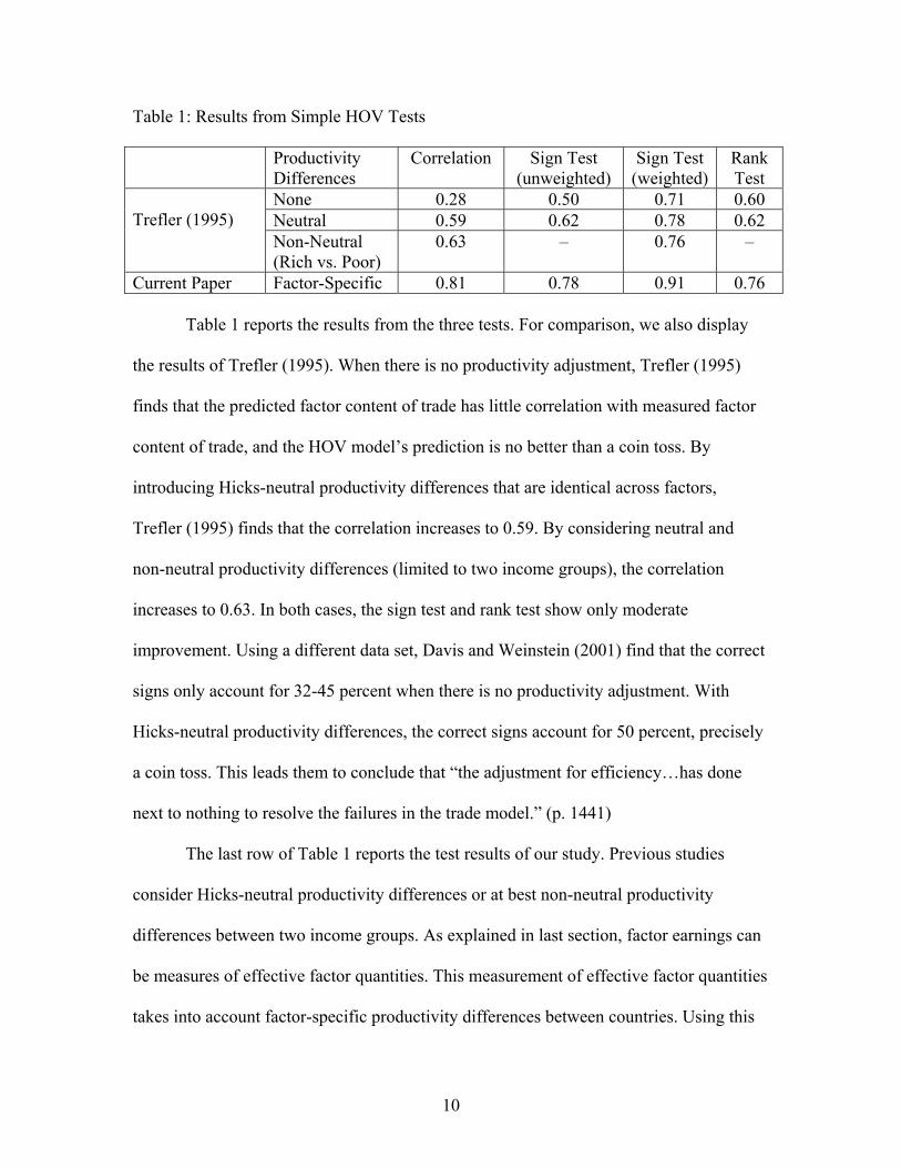
Table 1: Results from Simple HOV Tests

Productivity Differences

Correlation Sign Test (unweighted)

Sign Test (weighted)

Rank Test

None 0.28 0.50 0.71 0.60 Neutral 0.59 0.62 0.78 0.62

Trefler (1995)

Non-Neutral (Rich vs. Poor)

0.63 – 0.76 –

Current Paper Factor-Specific 0.81 0.78 0.91 0.76

Table 1 reports the results from the three tests. For comparison, we also display

the results of Trefler (1995). When there is no productivity adjustment, Trefler (1995)

finds that the predicted factor content of trade has little correlation with measured factor

content of trade, and the HOV model’s prediction is no better than a coin toss. By

introducing Hicks-neutral productivity differences that are identical across factors,

Trefler (1995) finds that the correlation increases to 0.59. By considering neutral and

non-neutral productivity differences (limited to two income groups), the correlation

increases to 0.63. In both cases, the sign test and rank test show only moderate

improvement. Using a different data set, Davis and Weinstein (2001) find that the correct

signs only account for 32-45 percent when there is no productivity adjustment. With

Hicks-neutral productivity differences, the correct signs account for 50 percent, precisely

a coin toss. This leads them to conclude that “the adjustment for efficiency…has done

next to nothing to resolve the failures in the trade model.” (p. 1441)

The last row of Table 1 reports the test results of our study. Previous studies

consider Hicks-neutral productivity differences or at best non-neutral productivity

differences between two income groups. As explained in last section, factor earnings can

be measures of effective factor quantities. This measurement of effective factor quantities

takes into account factor-specific productivity differences between countries. Using this

11

approach, we find the correlation between measured factor content of trade and predicted

factor content of trade to be 0.81. The unweighted sign test indicates that 78 percent of

the signs are correct. When more weights are attached to observations with large net

factor contents of trade, the sign test result is 0.91. The rank test result is 0.76. Taken

together, these results show that our consideration of factor-specific productivity

differences improves significantly the model’s fit to data. They provide support for our

using factor earnings as a proxy for effective factor quantities.

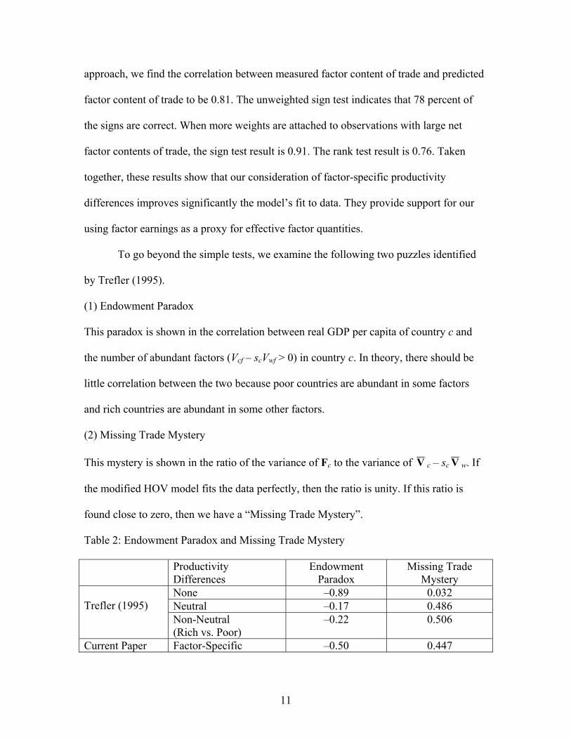
To go beyond the simple tests, we examine the following two puzzles identified

by Trefler (1995).

(1) Endowment Paradox

This paradox is shown in the correlation between real GDP per capita of country c and

the number of abundant factors (Vcf – scVwf > 0) in country c. In theory, there should be

little correlation between the two because poor countries are abundant in some factors

and rich countries are abundant in some other factors.

(2) Missing Trade Mystery

This mystery is shown in the ratio of the variance of Fc to the variance of V c – sc V w. If

the modified HOV model fits the data perfectly, then the ratio is unity. If this ratio is

found close to zero, then we have a “Missing Trade Mystery”.

Table 2: Endowment Paradox and Missing Trade Mystery Productivity

Differences Endowment

Paradox Missing Trade

Mystery None –0.89 0.032 Neutral –0.17 0.486

Trefler (1995)

Non-Neutral (Rich vs. Poor)

–0.22 0.506

Current Paper Factor-Specific –0.50 0.447

12

Table 2 reports the results. Regarding “Endowment Paradox”, Trefler (1995) finds

that the correlation between the number of abundant factors and per capital GDP is a high

–0.89, but it decreases to about –0.20 after adjusting for neutral productivity differences

and non-neutral productivity differences between two income groups. Regarding

“Missing Trade Mystery”, Trefler (1995) finds that the variance ratio is only 0.032; there

is simply no variation in the measured factor content of trade. With neutral and non-

neutral productivity adjustments the variance ratio increases to about 0.5, which is a

significant improvement.

The last row of Table 2 reports results from our sample. The correlation is –0.50,

indicating that the endowment paradox still exists. The variance ratio is 0.447, lower than

the 0.5 obtained by Trefler (1995). Why are our results poorer than that of Trefler (1995)

considering that we take into account more productivity differences? How do we

reconcile the less successful results in Table 2 with the more successful results in Table 1?

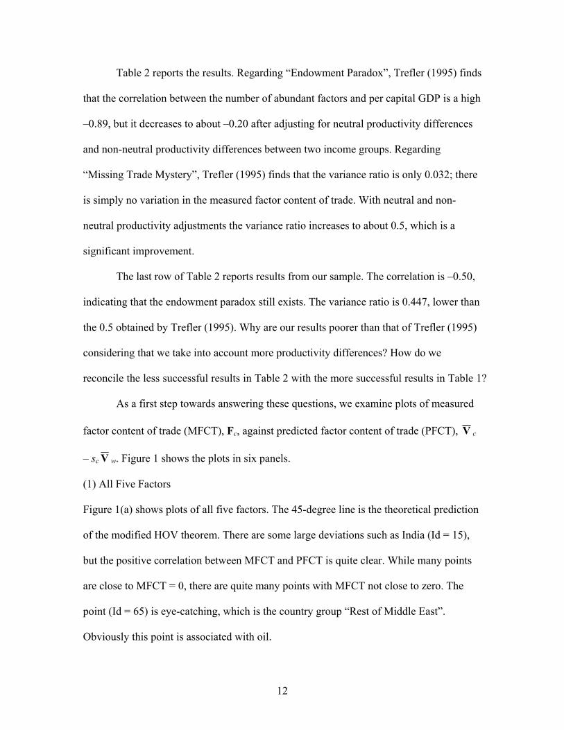
As a first step towards answering these questions, we examine plots of measured

factor content of trade (MFCT), Fc, against predicted factor content of trade (PFCT), V c

– sc V w. Figure 1 shows the plots in six panels.

(1) All Five Factors

Figure 1(a) shows plots of all five factors. The 45-degree line is the theoretical prediction

of the modified HOV theorem. There are some large deviations such as India (Id = 15),

but the positive correlation between MFCT and PFCT is quite clear. While many points

are close to MFCT = 0, there are quite many points with MFCT not close to zero. The

point (Id = 65) is eye-catching, which is the country group “Rest of Middle East”.

Obviously this point is associated with oil.

13

111

11 222223 333

34444

45

5

5

5 56 6

6

6 67 77

7788

8

889

9

9

99

10 10101010

11

11

11

1111

121212

1212 131313

131314 141414 14 15 15

1515 1516 1616161617 17

171717

1818

18

18 181919

19

191920

20

20

2020 2121

212121 2222

222222 2323232323

2424

24

2424 252525

2525 26262626 26 2727

2727 27 2828282828 29292929293030303030313131 3131

32

3232

323233 3333 3333343434

34343535

35

3535 3636

36

3636

373737 3737

3838

38383839 39393939

40

40

40

4040 41 4141414142 4242

424243 43434343 4444

44444445 4545

454546 4646464647 47

47

4747484848484849 4949

494950 5050505051515151515252525252535353535354 54545454 5555

555555565656565657 5757575758 58585858595959595960 60606060

6161

61

61 6162 62

6262626363636363 646464

6464

65

65

65

6565666666666667 67

67

67 6768

6868

6868696969

69 697070707070717171717172727272727373737373747474747475

75

75

7575767676767677 77

77

77 7778 787878 78

-20

020

4060

80M

easu

red

Fact

or C

onte

nt o

f Tra

de/

-20 0 20 40 60 80Predicted Factor Content of Trade

All Five Factors

Figure 1 (a)

1

23

4

5 6

7

89

10

11

12

131415

1617

18

19

20

21

2223

24

2526

2728293031

32

3334

3536

373839

40

414243

444546

47

4849

5051525354555657585960

61

6263

64

65

66

67

68 697071727374

75

76

77

78

-20

020

4060

80M

easu

red

Fact

or C

onte

nt o

f Tra

de/


Natural Resources

Figure 1 (b)

14

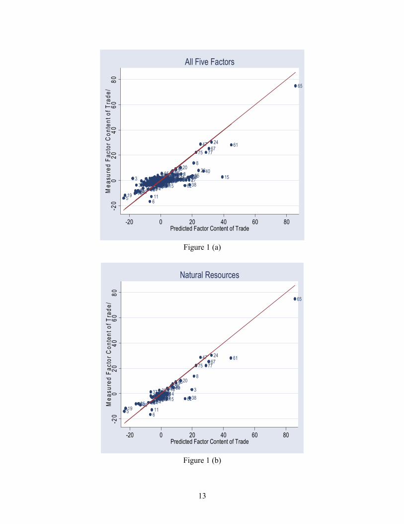
(2) Natural Resources

In our data, natural resources refer to cost value of non-producible natural source inputs

used in sectors of coal, oil, natural gas, minerals, fisheries and forestry. Figure 1(b) shows

that the modified HOV model explains the natural resource content of trade very well.

Our interpretation is that most of these natural resource items are traded in the world

market and hence have similar prices across countries. Because of this, factor earnings of

natural resources are good proxies for quantities of natural resources.

123

45 6789 1011

121314

1516 1718192021222324

25 262728293031

323334

353637

383940 4142 434445 4647 4849

50515253 54 555657585960 6162636465 66

676869 707172737475 7677 78

-10

010

2030

40M

easu

red

Fact

or C

onte

nt o

f Tra

de/


Land

Figure 1 (c)

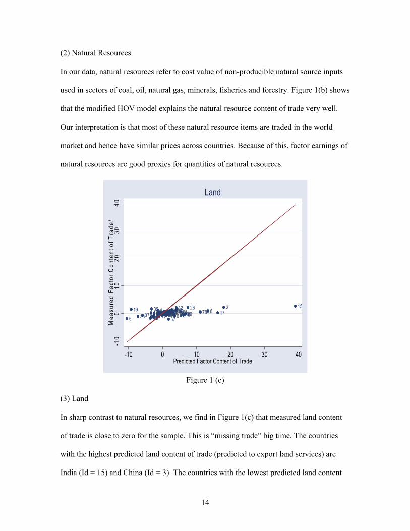
(3) Land

In sharp contrast to natural resources, we find in Figure 1(c) that measured land content

of trade is close to zero for the sample. This is “missing trade” big time. The countries

with the highest predicted land content of trade (predicted to export land services) are

India (Id = 15) and China (Id = 3). The countries with the lowest predicted land content

15

of trade (predicted to import land services) are the U.S. (Id = 19) and Japan (Id = 5). This

finding is at odds with the fact that China is scarce in land and the U.S. is abundant in

land. It suggests that the effective amount of land is greatly overestimated for India and

China, and greatly underestimated for the U.S. We will discuss this later.

123

4

5

67

89

10

11

12

1314

1516 17

1819

20

21

22 23

24

25 26 27282930

31

32

3334

3536

37 3839

40

4142434445 4647 4849

50515253

54555657585960

61

6263

64

65

6667

6869

70717273

74

75

7677 78

-20

-10

010

2030

Mea

sure

d Fa

ctor

Con

tent

of T

rade

/

-20 -10 0 10 20 30Predicted Factor Content of Trade

Capital

Figure 1 (d)

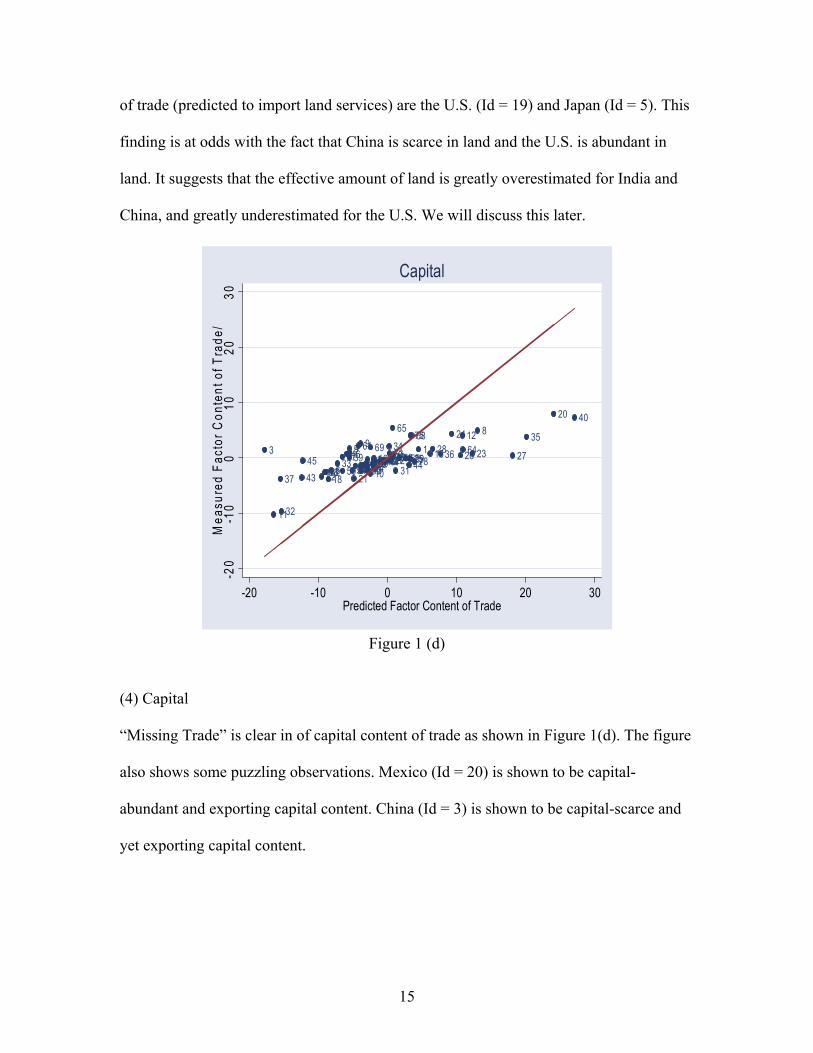
(4) Capital

“Missing Trade” is clear in of capital content of trade as shown in Figure 1(d). The figure

also shows some puzzling observations. Mexico (Id = 20) is shown to be capital-

abundant and exporting capital content. China (Id = 3) is shown to be capital-scarce and

yet exporting capital content.

16

123

4

5

67

8 9101112131415 1617

18

19

20 212223242526 2728 293031 32

33343536

37383940 4142 4344

4546

474849505152 535455 56 5758596061 62 63

6465

6667 6869707172737475767778

-10

010

20M

easu

red

Fact

or C

onte

nt o

f Tra

de/

-10 0 10 20Predicted Factor Content of Trade

Skilled Labor

Figure 1 (e)

12

3

4

5

6

7

8

9

10

11

1213

1415 1617 1819

20 21

2223 2425 262728 293031

32

333435

36

37383940 41

424344

454647

4849505152 5354

555657585960

616263

6465

66 6768

69707172737475 767778

-10

010

20M

easu

red

Fact

or C

onte

nt o

f Tra

de/


Unskilled Labor

Figure 1 (f)

17

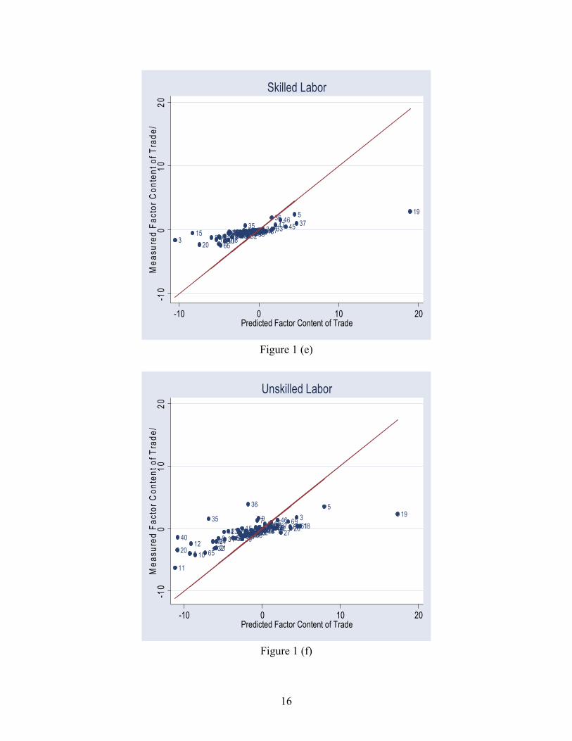
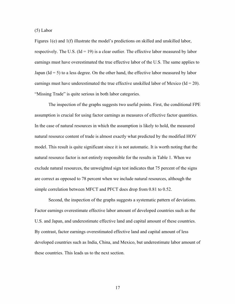
(5) Labor

Figures 1(e) and 1(f) illustrate the model’s predictions on skilled and unskilled labor,

respectively. The U.S. (Id = 19) is a clear outlier. The effective labor measured by labor

earnings must have overestimated the true effective labor of the U.S. The same applies to

Japan (Id = 5) to a less degree. On the other hand, the effective labor measured by labor

earnings must have underestimated the true effective unskilled labor of Mexico (Id = 20).

“Missing Trade” is quite serious in both labor categories.

The inspection of the graphs suggests two useful points. First, the conditional FPE

assumption is crucial for using factor earnings as measures of effective factor quantities.

In the case of natural resources in which the assumption is likely to hold, the measured

natural resource content of trade is almost exactly what predicted by the modified HOV

model. This result is quite significant since it is not automatic. It is worth noting that the

natural resource factor is not entirely responsible for the results in Table 1. When we

exclude natural resources, the unweighted sign test indicates that 75 percent of the signs

are correct as opposed to 78 percent when we include natural resources, although the

simple correlation between MFCT and PFCT does drop from 0.81 to 0.52.

Second, the inspection of the graphs suggests a systematic pattern of deviations.

Factor earnings overestimate effective labor amount of developed countries such as the

U.S. and Japan, and underestimate effective land and capital amount of these countries.

By contrast, factor earnings overestimated effective land and capital amount of less

developed countries such as India, China, and Mexico, but underestimate labor amount of

these countries. This leads us to the next section.

18

4. Factor Price Equalization Clubs

In this section we examine further the systematic deviations in our data. We argue that a

model of factor price equalization clubs may explain much of the deviations.

One crucial assumption of the modified HOV model is conditional FPE. Suppose

this assumption does not hold; instead, assume that countries are located in multiple

diversification cones which we call “Conditional FPE Clubs” or “FPE Clubs” for

simplicity. How does this affect our results? To see the logic, we use a simple example.

Under conditional FPE, we have wL and rK measuring effective labor and capital of

China, w*L* and r*K* measuring effective labor and capital of the U.S. Here

w/a=w*/a*= w =1 and r/b=r*/b*= r =1, where w and r are the factor prices in the

reference country normalized to be one, and a, a*, b, b* are productivity parameters.

Now consider the case with no conditional FPE. Labor is so abundant in China and

capital is so abundant in the U.S. that w/a<w*/a* and r/b>r*/b* in equilibrium. With the

reference country having the world average factor abundance, we have w<a, w*>a*, r>b,

and r*<b*. Therefore, wage earning (wL) underestimates China’s effective labor (aL)

while capital earning (rK) overestimates China’s effective capital (bK). For the same

logic, wage earning (w*L*) overestimates U.S.’s effective labor (a*L*) while capital

earning (r*K*) underestimates U.S.’s effective capital (b*K*).

It is difficult to identify FPE clubs from the data. What we do is to divide the

sample into groups according to real GDP per capita and examine results from the

subsamples to gain some insight. As a first step, we divide the sample into three groups.

The high-income group contains 24 countries with real GDP per capita (Penn World

Table 6.1) in 1997 exceeding $15,000. The middle-income group contains 30 countries

19

with real GDP per capita between $5,000 and $15,000. The low-income group contains

24 countries with real GDP per capita below $5,000.

Table 3: Results from Three Income Groups Endowment Paradox Missing Trade Mystery Full Sample (78) –0.50 0.447 High-Income Sample (24) 0.08 0.499 Middle-Income Sample (30) –0.12 0.552 Low-Income Sample (24) 0.001 0.600 Note: The number in parentheses is the number of countries in the sample.

Table 3 reports the results. Once we divide the sample into three income groups,

we find that the endowment paradox is largely resolved. Recall that the endowment

paradox refers to a strong negative correlation between the number of abundant factors

and GDP per capita—poor countries are found to be abundant in almost all factors and

rich countries are found to be scarce in almost all factors. Table 3 shows that there is little

correlation between the number of abundant factors and GDP per capita in all three

income groups. Notice also that the variance ratio, which is a measure of “Missing

Trade”, sees an improvement in all three groups.

The result on the endowment paradox can be explained as follows. As we

discussed above, in a multi-cone world, our measures of effective factor quantity

overestimate or underestimate factor abundance. For two countries in different FPE clubs,

the measurement biases apply to different factors. For countries in the same FPE club,

however, the measurement biases apply to the same factors. Thus the measurement biases

can affect significantly the correlation between the number of abundant factors and GDP

per capita in a sample of countries that belong to different income groups, but it would

have little effect on this correlation in a sample of countries that belong to a FPE club.

The evidence reported in Table 3 is consistent with this reasoning.

20

Table 3 shows the variance ratio of 0.5-0.6, which is quite remarkable considering

that the missing trade mystery has a lot to do with the preference side, which has not been

considered so far. As a robustness check of the results in Table 3, we report in Table 4 the

results when the sample is divided equally into four income groups.

Table 4: Results from Four Income Groups Endowment Paradox Missing Trade Mystery High-Income Sample (19) –0.098 0.548 High Middle-Income Sample (20) 0.122 0.380 Low Middle-Income Sample (19) –0.020 0.451 Low-Income Sample (20) –0.058 0.675 Note: The number in parentheses is the number of countries in the sample. The income thresholds are $20500, $8000, and $4000.

1

24

5

7

11

18

19

31

32

33

34

3536

3739

40

41

4244

4546

47

63

-20

-10

010

2030

Mea

sure

d Fa

ctor

Con

tent

of T

rade

/

-10 0 10 20 30Predicted Factor Content of Trade

High-Income Countries: Natural Resources

Figure 2 (a)

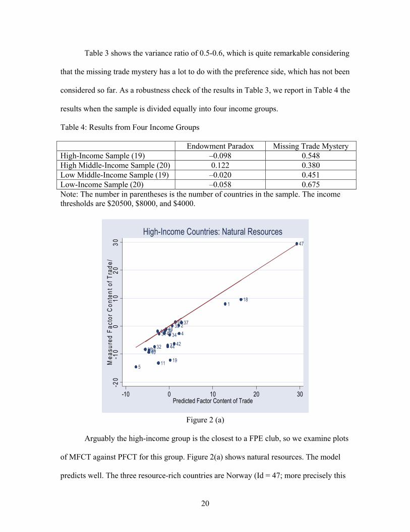
Arguably the high-income group is the closest to a FPE club, so we examine plots

of MFCT against PFCT for this group. Figure 2(a) shows natural resources. The model

predicts well. The three resource-rich countries are Norway (Id = 47; more precisely this

21

is a country group named “Rest of EFTA” that also includes Iceland and Liechtenstein),

Canada (Id = 18) and Australia (Id = 1). Measured natural resource contents of trade of

these three countries are close to what the model predicts. Not surprisingly, the majority

of high-income counties are net importers of natural resource content.

1

2

4

5

711

18

19

31

32

33

34

35

36

37

39

40

41

42

4445 464763

-20

-10

010

2030

Mea

sure

d Fa

ctor

Con

tent

of T

rade

/


High-Income Countries: Land

Figure 2 (b)

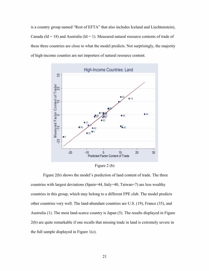
Figure 2(b) shows the model’s prediction of land content of trade. The three

countries with largest deviations (Spain=44, Italy=40, Taiwan=7) are less wealthy

countries in this group, which may belong to a different FPE club. The model predicts

other countries very well. The land-abundant countries are U.S. (19), France (35), and

Australia (1). The most land-scarce country is Japan (5). The results displayed in Figure

2(b) are quite remarkable if one recalls that missing trade in land is extremely severe in

the full sample displayed in Figure 1(c).

22

124

5

7

11

18

3132

333435

36

37

3940 414244

45

46

47

63

-20

-10

010

20M

easu

red

Fact

or C

onte

nt o

f Tra

de/

-20 -10 0 10 20Predicted Factor Content of Trade

High-Income Countries: Skilled Labor

Figure 2 (c)

12

4

5

7

11

18

3132

333435

36

37

3940 4142

444546

4763

-20

-10

010

20M

easu

red

Fact

or C

onte

nt o

f Tra

de/


High-Income Countries: Unskilled Labor

Figure 2 (d)

23

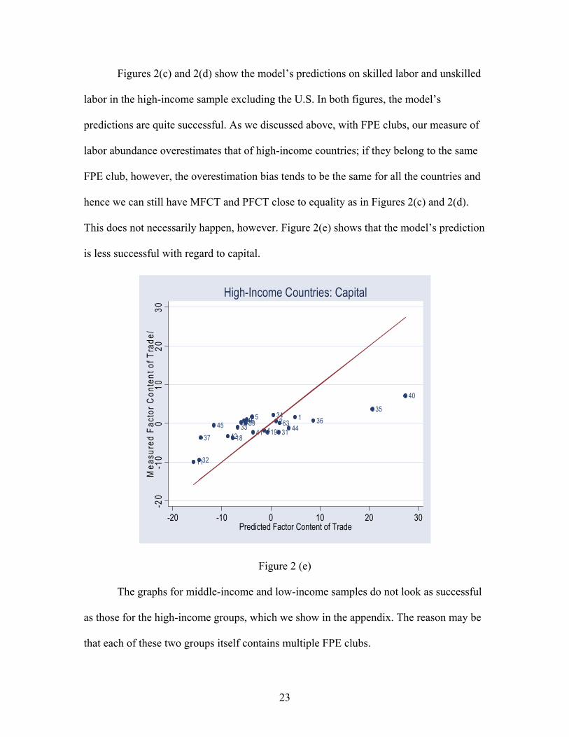
Figures 2(c) and 2(d) show the model’s predictions on skilled labor and unskilled

labor in the high-income sample excluding the U.S. In both figures, the model’s

predictions are quite successful. As we discussed above, with FPE clubs, our measure of

labor abundance overestimates that of high-income countries; if they belong to the same

FPE club, however, the overestimation bias tends to be the same for all the countries and

hence we can still have MFCT and PFCT close to equality as in Figures 2(c) and 2(d).

This does not necessarily happen, however. Figure 2(e) shows that the model’s prediction

is less successful with regard to capital.

124

57

11

1819 31

32

3334

3536

37

39

40

41424445 4647 63

-20

-10

010

2030

Mea

sure

d Fa

ctor

Con

tent

of T

rade

/


High-Income Countries: Capital

Figure 2 (e)

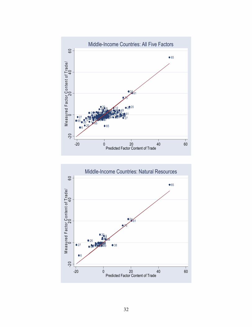
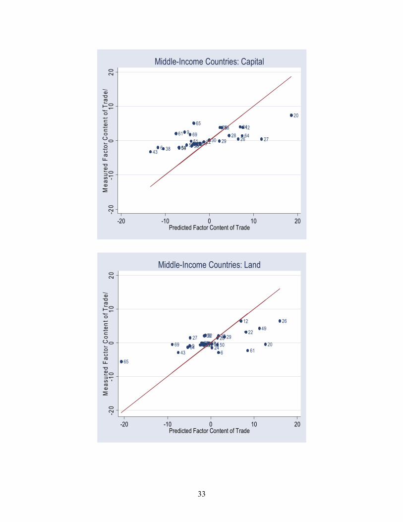
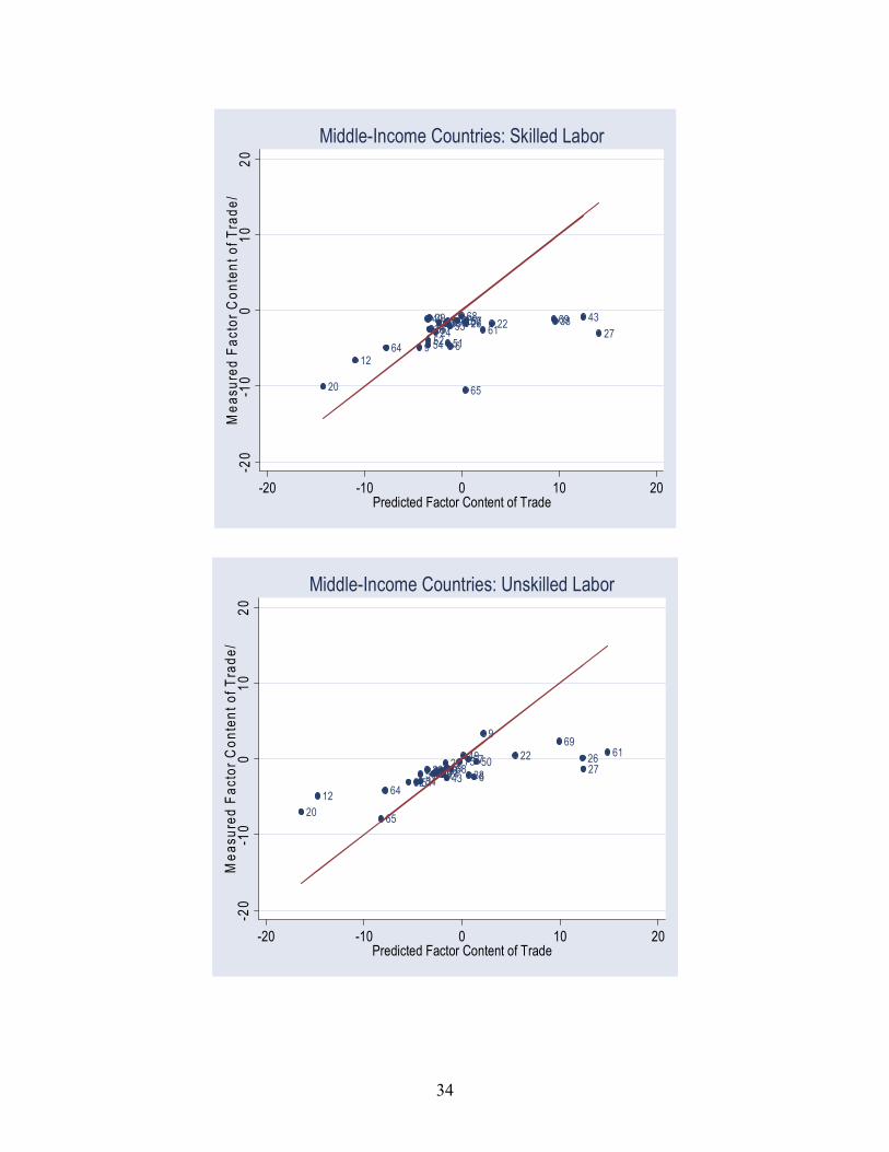
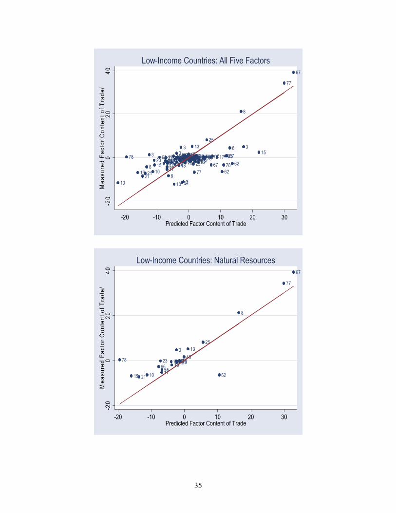
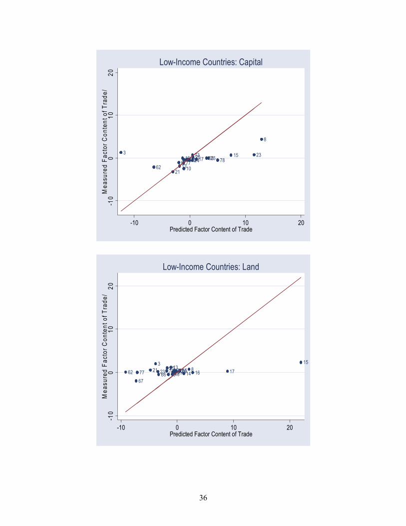
The graphs for middle-income and low-income samples do not look as successful

as those for the high-income groups, which we show in the appendix. The reason may be

that each of these two groups itself contains multiple FPE clubs.

24

5. Summary and Conclusion

This paper examines the role of factor productivity differences in explaining global trade.

Trade economists have used the Heckscher-Ohlin model as a main analytical framework

for trade issues, but data does not support the model’s empirical predictions on factor

content of trade. One explanation for its failure is that it does not consider cross-country

differences in factor productivity. Empirical evidence for this explanation is mixed. There

is evidence that factor productivity adjustment improves significantly the model’s fit to

data (e.g. Trefler, 1993, 1995), and there is evidence that it helps little of the model’s fit

(e.g. Davis and Weinstein, 2001).

One limitation of the existing studies is that productivity adjustment is limited to

Hicks-neutral productivity differences which are identical across factors, or at most

productivity differences that are non-neutral only between two country groups. This

limitation may have resulted in inaccurate measurement of effective factor quantities of a

country, partially responsible for the empirical failure of the model.

In this paper we aim to capture a wider range of factor productivity differences.

We adopt an approach that uses factor earnings to measure effective factor quantities.

The theoretical basis of this approach is that, under conditional FPE (factor price

equalization conditional on factor productivity differences), the relative productivity of a

factor in two countries equals the relative price of the factor in the two countries, so the

effective factor prices of the two countries are the same. This approach has an empirical

advantage: it does not require data on factor productivities or factor prices; all is needed

is the information on payments to factors.

25

The Global Trade Analysis Project (GTAP 5.4) provides such data. We use the

GTAP data to perform some standard tests on the HOV model modified with factor

productivity differences. Our results show that the correlation between measured factor

content of trade and predicted factor content of trade is 0.81. The sign of measure factor

content of trade matches the sign of predicted factor content of trade 78 percent of the

time when unweighted or 91 percent of the time when weighted by the size of factor

content of trade, a significant improvement over previous estimates based on Hicks-

neutral or two-group productivity adjustments. These results seem to suggest that

adjustment of factor-specific productivity differences can lead to a significant

improvement in the HOV model’s fit to data.

A further examination of the data identifies important deviations of the empirical

estimates from the model. The “Endowment Paradox” and “Missing Trade Mystery”, two

puzzles identified by Trefler (1995), still exist in our data with productivity adjustment.

The number of abundant factors of a country is smaller the higher the country’s GDP per

capita; the correlation between the two is –0.5. The variance of measured factor content

of trade is only 44.7 percent of the variance of the predicted factor content of trade, while

much higher than the “missing trade” value of 3.2 percent in Trefler’s data with no

productivity adjustment, fares no better than the 48.6 percent in Trefler’s data with

Hicks-neutral productivity adjustment.

Inspection of the deviations of the estimated factor content of trade allows us to

identify some patterns. Our measures of productivity-adjusted factor endowments tend to

overestimate the labor endowments of high-income countries but underestimate their land

and capital endowments. Our measures of productivity-adjusted factor endowments tend

26

to underestimate the labor endowments of low-income countries but overestimate their

land and capital endowments. In addition, for the production factor of natural resources,

we find that the model’s prediction fits the data extremely well.

We explain the regularities and anomalies in our results with a multi-cone model

in which countries belong to different “conditional FPE clubs”. Because many natural

resource items are traded, the assumption of conditional FPE holds for this factor and

hence we see a success of the HOV model with regard to this production factor. Because

in a multi-cone world labor scarcity of the high-income countries drives wage rates way

above those of the low-income countries, wage earnings in the high-income countries

overestimate productivity-adjusted labor quantities, while the opposite is true for land and

capital, our measures of effective factor quantities are biased, which explains why they

do not fare well with the “Endowment Paradox” test and “Missing Trade” test which are

based largely on between-country factor quantity comparisons. On the other hand, the

correlations and sign matches are more successful because they are affected less by

between-country factor quantity comparisons.

We find further evidence to support our explanation. When we split the sample

into three or four income groups, we find that the endowment paradox disappears. This is

because our factor measures are biased in a systematic way; the bias is the same for the

countries in the same FPE club and hence the measurement of factor abundance between

them does not exhibit a correlation between factor abundance and GDP per capita. We

also find some improvement in resolving the missing trade mystery; the variance ratios

increase to 0.5-0.6 when we apply the variance test to income-group samples.

27

Arguably the group of high-income countries is the closest among all country

groups to a conditional FPE club. Our results support this view. We find that the

modified HOV model gives much better predictions for the high-income sample than the

full sample or the middle-income or low-income samples.

We draw two conclusions: (1) Productivity adjustment needs to be adequately

done to judge the validity of the HOV model. Previous studies may have underestimated

the significance of factor productivity adjustment in improving the fit of the HOV model.

(2) There are patterns in the deviations of the estimates from the HOV model with

conditional FPE, which may be explained by considering “conditional FPE clubs”.

28

References

Bowen, Harry P., Edward E. Leamer, and Leo Sveikauskas (1987), “Multicountry, Multifactor Tests of the Factor Abundance Theory,” American Economic Review, 77 (5), 791-809. Davis, Donald R. and David E. Weinstein (2003), “The Factor Content of Trade,” in E. Kwan Choi and james Harrigan, eds., Handbook of International Trade, Blackwell Publishing, 119-145. Davis, Donald R. and David E. Weinstein (2001), “An Account of Global Factor Trade,” American Economic Review, 91 (5), 1423-1453. Krugman, Paul R. and Maurice Obstfeld (2003), International Economics: Theory and Policy, 6th Edition, Addison-Wesley. Leamer, Edward E. (1980), “The Leontief Paradox, Reconsidered,” Journal of Political Economy, 88, 495-503. Leontief, Wassily (1953), “Domestic Production and Foreign Trade: The American Capital Position Re-Examined,” Proceedings of the American Philosophical Society, 97, 332-349. Trefler, Daniel (1995), “The Case of Missing Trade and Other Mysteries,” American Economic Review, 85 (5), 1029-1046. Trefler, Daniel (1993), “International Factor Price Differences: Leontief Was Right!” Journal of Political Economy, 101, 961-987. Trefler, Daniel and Susan Chun Zhu (2000), “Beyond the Algebra of Explanation: HOV for the Technology Age,” American Economic Review, 90, 145-149.

29

Appendix

1. Data Summary

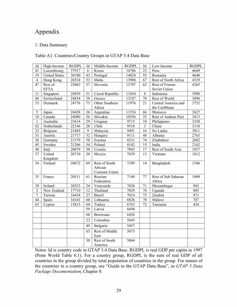
Table A1: Countries/Country Groups in GTAP 5.4 Data Base

Id High-Income RGDPL Id Middle-Income RGDPL Id Low-Income RGDPL 41 Luxembourg 37917 6 Korea 14786 23 Peru 4649 19 United States 30190 43 Portugal 14024 55 Romania 4640 4 Hong Kong 26524 53 Malta 13908 67 Rest of North Africa 4319

47 Rest of EFTA

25862 57 Slovenia 13787 62 Rest of Former Soviet Union

4265

11 Singapore 24939 51 Czech Republic 13454 8 Indonesia 3990 46 Switzerland 24834 38 Greece 13187 78 Rest of World 3896 33 Denmark 24776 75 Other Southern

Africa 11976 21 Central America and

the Caribbean 3752

5 Japan 24428 26 Argentina 11354 66 Morocco 3627 18 Canada 24080 56 Slovakia 10556 25 Rest of Andean Pact 3413 1 Australia 23614 29 Uruguay 9715 10 Philippines 3358

42 Netherlands 22146 28 Chile 9518 3 China 3110 32 Belgium 21845 9 Malaysia 9491 16 Sri Lanka 3011 31 Austria 21717 52 Hungary 9111 48 Albania 2763 36 Germany 21379 58 Estonia 8231 74 Zimbabwe 2682 45 Sweden 21266 54 Poland 8142 15 India 2162 40 Italy 20879 50 Croatia 7843 17 Rest of South Asia 1837 37 United

Kingdom 20710 20 Mexico 7639 13 Vietnam 1812

34 Finland 20672 69 Rest of South African Customs Union

7189 14 Bangladesh 1546

35 France 20511 61 Russian Federation

7149 77 Rest of Sub Saharan Africa

1009

39 Ireland 20323 24 Venezuela 7038 71 Mozambique 943 2 New Zealand 17710 12 Thailand 7029 76 Uganda 885 7 Taiwan 16434 27 Brazil 7014 73 Zambia 871

44 Spain 16141 60 Lithuania 6826 70 Malawi 787 63 Cyprus 15813 64 Turkey 6763 72 Tanzania 424

59 Latvia 6698 68 Botswana 6428 22 Colombia 5645 49 Bulgaria 5457 65 Rest of Middle

East 5073

30 Rest of South America

5064

Notes: Id is country code in GTAP 5.4 Data Base. RGDPL is real GDP per capita in 1997 (Penn World Table 6.1). For a country group, RGDPL is the sum of real GDP of all countries in the group divided by total population of countries in the group. For names of the countries in a country group, see “Guide to the GTAP Data Base”, in GTAP 5 Data Package Documentation, Chapter 8.

30

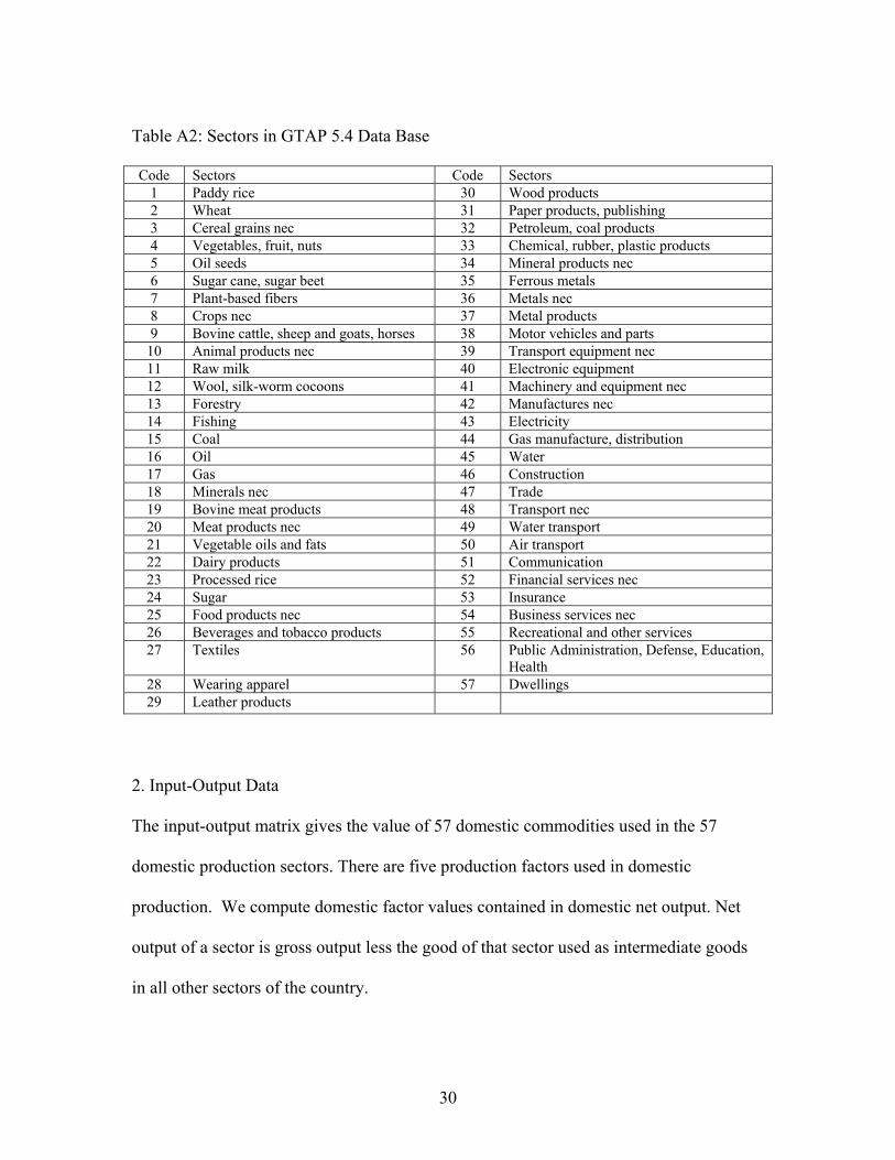
Table A2: Sectors in GTAP 5.4 Data Base Code Sectors Code Sectors

1 Paddy rice 30 Wood products 2 Wheat 31 Paper products, publishing 3 Cereal grains nec 32 Petroleum, coal products 4 Vegetables, fruit, nuts 33 Chemical, rubber, plastic products 5 Oil seeds 34 Mineral products nec 6 Sugar cane, sugar beet 35 Ferrous metals 7 Plant-based fibers 36 Metals nec 8 Crops nec 37 Metal products 9 Bovine cattle, sheep and goats, horses 38 Motor vehicles and parts

10 Animal products nec 39 Transport equipment nec 11 Raw milk 40 Electronic equipment 12 Wool, silk-worm cocoons 41 Machinery and equipment nec 13 Forestry 42 Manufactures nec 14 Fishing 43 Electricity 15 Coal 44 Gas manufacture, distribution 16 Oil 45 Water 17 Gas 46 Construction 18 Minerals nec 47 Trade 19 Bovine meat products 48 Transport nec 20 Meat products nec 49 Water transport 21 Vegetable oils and fats 50 Air transport 22 Dairy products 51 Communication 23 Processed rice 52 Financial services nec 24 Sugar 53 Insurance 25 Food products nec 54 Business services nec 26 Beverages and tobacco products 55 Recreational and other services 27 Textiles 56 Public Administration, Defense, Education,

Health 28 Wearing apparel 57 Dwellings 29 Leather products

2. Input-Output Data

The input-output matrix gives the value of 57 domestic commodities used in the 57

domestic production sectors. There are five production factors used in domestic

production. We compute domestic factor values contained in domestic net output. Net

output of a sector is gross output less the good of that sector used as intermediate goods

in all other sectors of the country.

31

3. Trade Data

For each country, there are data of exports of 57 domestic sectors to 77 other countries,

measured in world prices. We use the data to compute factor content of a country’s

exports to all other countries. From this we obtain factor content of imports of a given

country.

4. Factor Units

For factors to be expressed in comparable units (to satisfy the statistical hypothesis of

homoscedasticity), we follow Trefler (1995) to scale the data by σfsc1/2, where σf is the

standard error of εcf = Fcf – (Vcf – scVwf).

5. Primary Factors

The split between skilled and unskilled labor is on the basis of occupational

classifications of the International Labor Organization (ILO). For details, see “Skilled

and Unskilled Labor Data”, in GTAP 5 Data Package Documentation, Chapter 18.D. For

natural resources, see “Primary Factor Shares”, Chapter 18.C. For capital stock data, see

“Capital Stock and Depreciation”, Chapter 18.B.

6. Additional Results

The following are graphs for the Middle-Income Sample and Low-Income Sample.

32

6 6

6

66

99

9

9

9 1212

121212

20

20

20

2020

222222

2222

24

24

24

242426

2626

26 26272727 2727

2828282828 2929292929303030303038

3838 383843 4343 434349

49

4949 4950 5050 5050515151

515152

52525252

535353535354 545454545656

56565657 5757 575758 58585858595959595960 60606060

6161

61

616164

6464 6464

65

65

65

6565

6868

686868

6969

69696975

75

75

7575

-20

020

4060

Mea

sure

d Fa

ctor

Con

tent

of T

rade

/


Middle-Income Countries: All Five Factors

6

9

12

2022

24

2627

282930 3843 49505152 53545657 585960

61

64

65

6869

75

-20

020

4060

Mea

sure

d Fa

ctor

Con

tent

of T

rade

/


Middle-Income Countries: Natural Resources

33

6

912

20

22

24

26 2728

29303843

4950

51525354

5657585960

61 64

6568

6975

-20

-10

010

20M

easu

red

Fact

or C

onte

nt o

f Tra

de/


Middle-Income Countries: Capital

69

12

20

22

24

26

27 28 293038

43

49

505152

53 545657 5859606164

65

6869 75

-20

-10

010

20M

easu

red

Fact

or C

onte

nt o

f Tra

de/


Middle-Income Countries: Land

34

6912

20

2224

262728

2930 38 4349 50

515253

5456

57585960 6164

65

68 6975

-20

-10

010

20M

easu

red

Fact

or C

onte

nt o

f Tra

de/


Middle-Income Countries: Skilled Labor

6

9

1220

2224

262728 29

30 3843

49 50

515253

545657

585960

61

64

65

68

69

75

-20

-10

010

20M

easu

red

Fact

or C

onte

nt o

f Tra

de/


Middle-Income Countries: Unskilled Labor

35

3 33

3

388

8

8

810

10

10

1010

1313

13

1313141414 14 14 15

15

1515

15 16 1616 161617 17

171717

2121

21

2121

2323232323 2525

25

2525 4848484848 5555

55 55556262

6262626666

66 66666767

67

67

67707070 70 7071717171 7172727272 72737373 7373747474 747476767676 767777

77

77

7778787878

78

-20

020

40M

easu

red

Fact

or C

onte

nt o

f Tra

de/


Low-Income Countries: All Five Factors

3

8

10

13

14

15

1617

21

23

25

48

5562

66

67

707172737476

77

78

-20

020

40M

easu

red

Fact

or C

onte

nt o

f Tra

de/


Low-Income Countries: Natural Resources

36

3

8

101314

1516 17

21

232548 55

626667

70717273

747677 78

-10

010

20M

easu

red

Fact

or C

onte

nt o

f Tra

de/


Low-Income Countries: Capital

38

1013

14

15

16 1721 2325

485562 66

67

7071727374 7677 78

-10

010

20M

easu

red

Fact

or C

onte

nt o

f Tra

de/


Low-Income Countries: Land

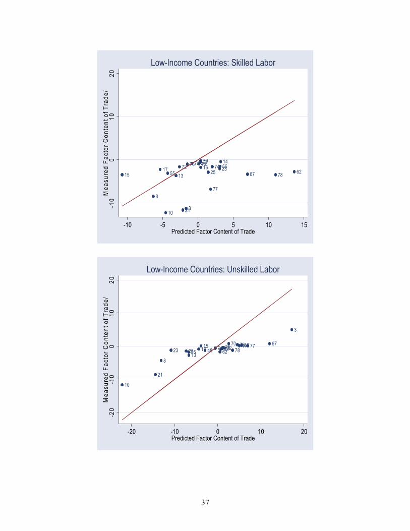
37

3

8

10

13

14

151617

21

232548

55 6266

67

707172

737476

77

78

-10

010

20M

easu

red

Fact

or C

onte

nt o

f Tra

de/


Low-Income Countries: Skilled Labor

3

8

10

13

1415 1617

21

23 25 4855 6266 6770

7172737476 77

78

-20

-10

010

20M

easu

red

Fact

or C

onte

nt o

f Tra

de/


Low-Income Countries: Unskilled Labor

Documents

Factor Productivity and Global Trade - CEIBS