Factors Affecting an Individual’s Future Labour Market … · Factors Affecting an Individual’s Future ... FACTORS AFFECTING AN INDIVIDUAL’S FUTURE LABOUR MARKET STATUS

11BULLETIN | D E C E M B E R Q UA R T E R 2016

Factors Affecting an Individual’s Future Labour Market StatusMichelle van der Merwe*

This article examines the ways in which someone’s characteristics and circumstances in one year affect their probability of being in a particular labour market state in the next year. People are more likely to be employed next year if they are currently employed and have tertiary qualifications. In contrast, they are more likely to be unemployed or outside the labour force if they have a long-term health condition, have not completed high school or are a migrant from a non-English-speaking background. Additionally, the article considers the changing importance of determinants over time, noting the role that changes in individual and household preferences as well as broader macroeconomic conditions are likely to have played.

IntroductionUnderlying the changes in aggregate labour market outcomes there are much larger flows of individuals into and out of employment, unemployment and the labour force. Understanding the determinants of these flows can help to shed light on aggregate developments and refine an assessment of the degree of spare capacity in the labour market. For example, aggregate developments could reflect changes in the structure of the population or changes in the propensity of certain groups to participate in the labour market. An assessment could be made that the potential labour supply (as measured by the number of unemployed persons) may be smaller if the unemployed consists of individuals who are less likely to be matched to a job than others, given their characteristics. In contrast, if individuals outside the labour force, such as the marginally attached, display similar behaviour to those who are unemployed, then the potential supply of labour could be larger than otherwise (Gray, Heath and Hunter 2002).1

1 Marginal attachment refers to the individuals who are not currently actively looking for work, but want to work and are available to take up employment.

The purpose of this article is to understand how someone’s characteristics and circumstances affect the probability of being in a particular labour market state in the next year. Previous Australian studies have typically focused on the experience of particular groups of individuals or particular types of labour market flows rather than the aggregate labour market flows from year to year. For example, in addition to Gray et al (2002), who focused on the behaviour of individuals that are marginally attached to the labour market, Haynes, Western and Spallek (2005) examine the characteristics that influence the employment status of Australian women, while Carrol and Poehl (2007) investigate whether certain groups of individuals are more likely to separate voluntarily or involuntarily from their employer.

The remainder of this article describes the features of the data, with a particular emphasis on the nature of the labour market changes observed, before moving to a more formal modelling approach that allows the relative importance of factors associated with an individual’s future labour market status to be determined.

* The author is from Economic Analysis Department and is solely responsible for any errors. Thanks to Denzil Fiebig, Adam Gorajek and Gianni La Cava for their helpful comments and suggestions, including on earlier versions of this article.

EC Bulletin.indb 11 13/12/2016 10:29 am

12 RESERVE BANK OF AUSTRALIA

FACTORS AFFECTING AN INDIVIDUAL’S FUTURE LABOUR MARKET STATUS

The DataThe Household, Income and Labour Dynamics in Australia (HILDA) Survey is a longitudinal household study that collects information from Australian individuals and households about economic and subjective wellbeing, labour market dynamics and family dynamics. The survey is conducted on an annual basis and is designed to be representative of the Australian resident population. It follows individuals and households over time.

The HILDA Survey provides a suitable dataset to answer the broader objectives of this article because it provides a detailed breakdown of an individual’s labour market status each year as well as their individual characteristics. For the purpose of this article, four mutually exclusive labour market states are considered: employed; unemployed; marginally attached to the labour force; and not in the labour force (NILF) for reasons other than marginal attachment. Individuals who report their labour market status as self-employed or as participating in full-time study are excluded; the propensity for these individuals to transition between labour market states may reflect changes in very particular circumstances, such as business failure or the end of formal studies, both of which are outside the scope of this article. Further, individuals not present across two consecutive years of the survey are also excluded given the interest in labour market dynamics of this analysis.

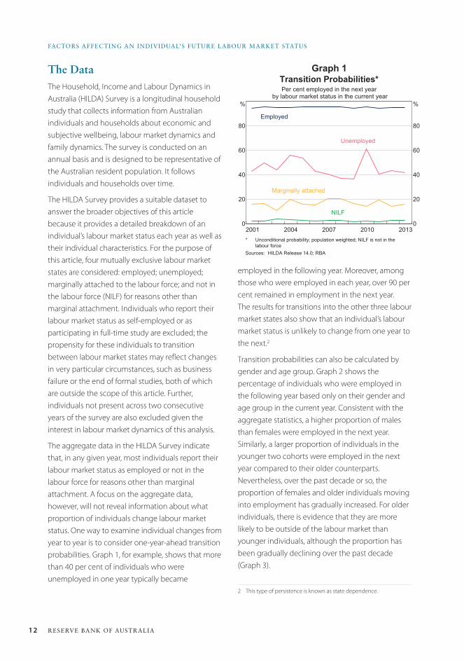
The aggregate data in the HILDA Survey indicate that, in any given year, most individuals report their labour market status as employed or not in the labour force for reasons other than marginal attachment. A focus on the aggregate data, however, will not reveal information about what proportion of individuals change labour market status. One way to examine individual changes from year to year is to consider one-year-ahead transition probabilities. Graph 1, for example, shows that more than 40 per cent of individuals who were unemployed in one year typically became

employed in the following year. Moreover, among those who were employed in each year, over 90 per cent remained in employment in the next year. The results for transitions into the other three labour market states also show that an individual’s labour market status is unlikely to change from one year to the next.2

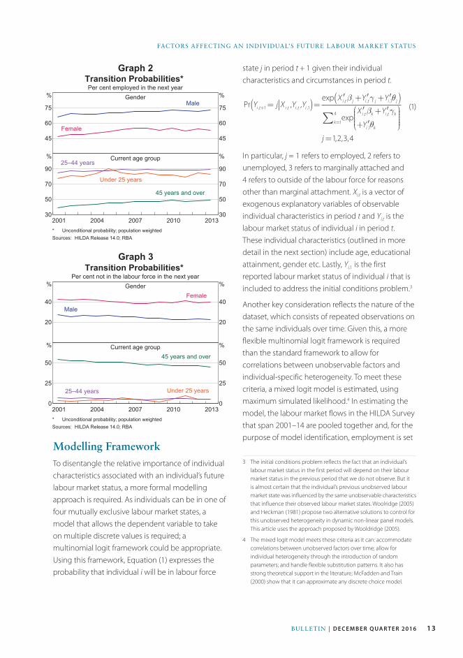
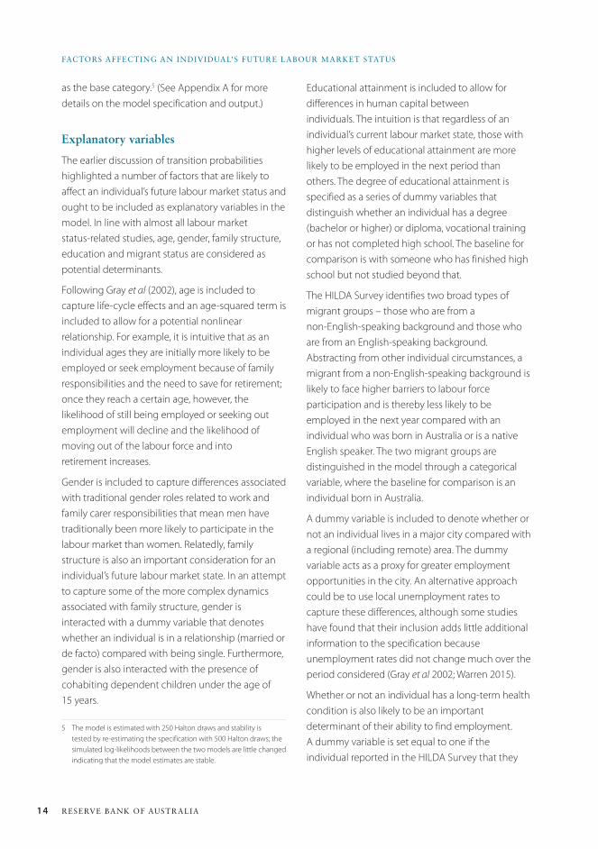
Transition probabilities can also be calculated by gender and age group. Graph 2 shows the percentage of individuals who were employed in the following year based only on their gender and age group in the current year. Consistent with the aggregate statistics, a higher proportion of males than females were employed in the next year. Similarly, a larger proportion of individuals in the younger two cohorts were employed in the next year compared to their older counterparts. Nevertheless, over the past decade or so, the proportion of females and older individuals moving into employment has gradually increased. For older individuals, there is evidence that they are more likely to be outside of the labour market than younger individuals, although the proportion has been gradually declining over the past decade (Graph 3).

2 This type of persistence is known as state dependence.

Graph 1

2010200720042001 20130

20

40

60

80

%

0

20

40

60

80

%

Transition Probabilities*Per cent employed in the next year

by labour market status in the current year

Employed

Unemployed

Marginally attached

NILF

* Unconditional probability; population weighted; NILF is not in thelabour force

Sources: HILDA Release 14.0; RBA




state j in period t + 1 given their individual characteristics and circumstances in period t.

(1)

In particular, j = 1 refers to employed, 2 refers to unemployed, 3 refers to marginally attached and 4 refers to outside of the labour force for reasons other than marginal attachment. Xi,t is a vector of exogenous explanatory variables of observable individual characteristics in period t and Yi,t is the labour market status of individual i in period t. These individual characteristics (outlined in more detail in the next section) include age, educational attainment, gender etc. Lastly, Yi,1 is the first reported labour market status of individual i that is included to address the initial conditions problem.3

Another key consideration reflects the nature of the dataset, which consists of repeated observations on the same individuals over time. Given this, a more flexible multinomial logit framework is required than the standard framework to allow for correlations between unobservable factors and individual-specific heterogeneity. To meet these criteria, a mixed logit model is estimated, using maximum simulated likelihood.4 In estimating the model, the labour market flows in the HILDA Survey that span 2001–14 are pooled together and, for the purpose of model identification, employment is set

3 The initial conditions problem reflects the fact that an individual’s labour market status in the first period will depend on their labour market status in the previous period that we do not observe. But it is almost certain that the individual’s previous unobserved labour market state was influenced by the same unobservable characteristics that influence their observed labour market states. Woolridge (2005) and Heckman (1981) propose two alternative solutions to control for this unobserved heterogeneity in dynamic non-linear panel models. This article uses the approach proposed by Wooldridge (2005).

4 The mixed logit model meets these criteria as it can: accommodate correlations between unobserved factors over time; allow for individual heterogeneity through the introduction of random parameters; and handle flexible substitution patterns. It also has strong theoretical support in the literature; McFadden and Train (2000) show that it can approximate any discrete choice model.

Pr Yi ,t+1= j X i ,t ,Yi ,t ,Yi ,1( )=exp ′Xi ,tβ j+ ′Yi ,tγ j+ ′Yi ,1θ j( )

exp′Xi ,tβk+ ′Yi ,tγk+ ′Yi ,1θk

⎛

⎝⎜⎜⎜⎜

⎞

⎠

⎟⎟⎟⎟⎟k=1

4∑j=1,2,3,4

Graph 3Transition Probabilities*

Per cent not in the labour force in the next yearGender

20

40

%

20

40

%

Female

Male

Current age group

2010200720042001 20130

25

50

%

0

25

50

%

Under 25 years25–44 years

45 years and over

* Unconditional probability; population weightedSources: HILDA Release 14.0; RBA

Graph 2Transition Probabilities*Per cent employed in the next year

Gender

45

60

75

%

45

60

75

%Male

Female

Current age group

2010200720042001 201330

50

70

90

%

30

50

70

90

%

45 years and over

Under 25 years

25–44 years

* Unconditional probability; population weightedSources: HILDA Release 14.0; RBA

Modelling FrameworkTo disentangle the relative importance of individual characteristics associated with an individual’s future labour market status, a more formal modelling approach is required. As individuals can be in one of four mutually exclusive labour market states, a model that allows the dependent variable to take on multiple discrete values is required; a multinomial logit framework could be appropriate. Using this framework, Equation (1) expresses the probability that individual i will be in labour force




Educational attainment is included to allow for differences in human capital between individuals. The intuition is that regardless of an individual’s current labour market state, those with higher levels of educational attainment are more likely to be employed in the next period than others. The degree of educational attainment is specified as a series of dummy variables that distinguish whether an individual has a degree (bachelor or higher) or diploma, vocational training or has not completed high school. The baseline for comparison is with someone who has finished high school but not studied beyond that.

The HILDA Survey identifies two broad types of migrant groups – those who are from a non-English-speaking background and those who are from an English-speaking background. Abstracting from other individual circumstances, a migrant from a non-English-speaking background is likely to face higher barriers to labour force participation and is thereby less likely to be employed in the next year compared with an individual who was born in Australia or is a native English speaker. The two migrant groups are distinguished in the model through a categorical variable, where the baseline for comparison is an individual born in Australia.

A dummy variable is included to denote whether or not an individual lives in a major city compared with a regional (including remote) area. The dummy variable acts as a proxy for greater employment opportunities in the city. An alternative approach could be to use local unemployment rates to capture these differences, although some studies have found that their inclusion adds little additional information to the specification because unemployment rates did not change much over the period considered (Gray et al 2002; Warren 2015).

Whether or not an individual has a long-term health condition is also likely to be an important determinant of their ability to find employment. A dummy variable is set equal to one if the individual reported in the HILDA Survey that they

as the base category.5 (See Appendix A for more details on the model specification and output.)

Explanatory variables

The earlier discussion of transition probabilities highlighted a number of factors that are likely to affect an individual’s future labour market status and ought to be included as explanatory variables in the model. In line with almost all labour market status-related studies, age, gender, family structure, education and migrant status are considered as potential determinants.

Following Gray et al (2002), age is included to capture life-cycle effects and an age-squared term is included to allow for a potential nonlinear relationship. For example, it is intuitive that as an individual ages they are initially more likely to be employed or seek employment because of family responsibilities and the need to save for retirement; once they reach a certain age, however, the likelihood of still being employed or seeking out employment will decline and the likelihood of moving out of the labour force and into retirement increases.

Gender is included to capture differences associated with traditional gender roles related to work and family carer responsibilities that mean men have traditionally been more likely to participate in the labour market than women. Relatedly, family structure is also an important consideration for an individual’s future labour market state. In an attempt to capture some of the more complex dynamics associated with family structure, gender is interacted with a dummy variable that denotes whether an individual is in a relationship (married or de facto) compared with being single. Furthermore, gender is also interacted with the presence of cohabiting dependent children under the age of 15 years.

5 The model is estimated with 250 Halton draws and stability is tested by re-estimating the specification with 500 Halton draws; the simulated log-likelihoods between the two models are little changed indicating that the model estimates are stable.




had a long-term health condition, disability or impairment that restricted their everyday activities and could not be corrected by medication or medical aids.

Lastly, considerable attention in the literature has been devoted to the role of the current labour market state in explaining subsequent labour market outcomes (e.g. Prowse 2010). This so-called ’state dependence’ is closely related to the scarring hypothesis of unemployment whereby there is a causal link between past and current unemployment. As Arulampalam, Booth and Taylor (2000, p 25) explain, state dependence is such that ‘an individual who does not experience unemployment now will behave differently in the future to an otherwise identical individual currently experiencing unemployment’. Similarly, an individual who is currently employed is likely to be building up their stock of human capital, which in turn is likely to increase the probability of being employed in the future. To examine whether state dependence is a determinant of an individual’s future labour force status, for which the preliminary analysis also found strong supporting evidence, a categorical dummy variable indicating their labour market status in the current period is included in the model.6

Results As the coefficient estimates from the mixed logit model are not straightforward to interpret, average marginal effects are presented instead.7 These effects describe the change in the predicted probability of a particular outcome when an explanatory variable changes by one unit or, in the case of a binary variable, the variable changes from zero to one,

6 True state dependence is distinguished here from spurious dependence that stems from an individual’s unobservable attributes; both are separately controlled for in the mixed logit modelling framework so that the coefficients and average marginal effects associated with the current labour market status can be interpreted as the effect of true state dependence.

7 The sign and statistical significance of the coefficient estimates from the mixed logit regression are meaningful to interpret but not the magnitude of the coefficients themselves.

holding all other variables constant. As an individual can only be in one labour market state, the average marginal effects for each variable must sum to zero.

For the dummy variables in the model specification, the average marginal effect is calculated as the mean difference in the predicted probabilities of being in a given labour market state next year when the value of the variable is set to zero for all individuals in the sample, and when the variable is set to one for all individuals in the sample (holding all other explanatory variables constant). For the continuous variables, the average marginal effect is the mean change in the predicted probability when the value of the variable is increased by one unit and all other explanatory variables are held constant. The predicted probabilities under the different scenarios for the dummy and continuous variables are calculated through a series of simulation exercises that use the estimated mixed logit model; one consequence of this approach is that we are unable to comment on the statistical significance of the average marginal effects.8

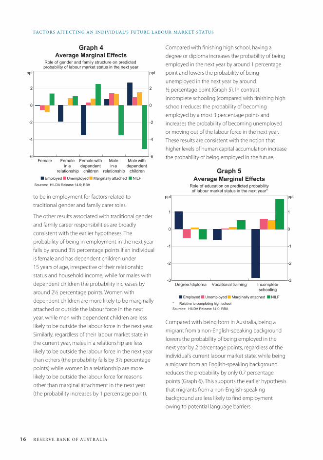
All other things being equal, being female increases the probability of being outside the labour force in the next year by around 1.4 percentage points. The result is in line with the aggregate data that consistently show that a higher proportion of women are outside the labour force than men in any given year; for example, because of earlier retirement or family carer responsibilities (Graph 4).9 In contrast, the probability of being employed in the next year is little different for females and males (that is the average marginal effect for females is close to zero), which is somewhat surprising given that men have historically had a higher propensity

8 To comment on whether the average marginal effect is statistically significant requires us to consider whether the corresponding regression coefficient in the mixed logit regression is statistically significant (refer to Appendix A).

9 In interpreting the average marginal effects associated with gender roles and family structure, the baseline comparison for females is males; the baseline comparison for females who are in a relationship is males and females who are not in a relationship; the baseline comparison for females with dependent children is males and females without dependent children; and so on.




to be in employment for factors related to traditional gender and family carer roles.

The other results associated with traditional gender and family career responsibilities are broadly consistent with the earlier hypotheses. The probability of being in employment in the next year falls by around 31/2 percentage points if an individual is female and has dependent children under 15 years of age, irrespective of their relationship status and household income; while for males with dependent children the probability increases by around 21/2 percentage points. Women with dependent children are more likely to be marginally attached or outside the labour force in the next year, while men with dependent children are less likely to be outside the labour force in the next year. Similarly, regardless of their labour market state in the current year, males in a relationship are less likely to be outside the labour force in the next year than others (the probability falls by 31/2 percentage points) while women in a relationship are more likely to be outside the labour force for reasons other than marginal attachment in the next year (the probability increases by 1 percentage point).

Compared with finishing high school, having a degree or diploma increases the probability of being employed in the next year by around 1 percentage point and lowers the probability of being unemployed in the next year by around 1/2 percentage point (Graph 5). In contrast, incomplete schooling (compared with finishing high school) reduces the probability of becoming employed by almost 3 percentage points and increases the probability of becoming unemployed or moving out of the labour force in the next year. These results are consistent with the notion that higher levels of human capital accumulation increase the probability of being employed in the future.

Graph 4

Graph 5

Average Marginal EffectsRole of gender and family structure on predictedprobability of labour market status in the next year

Female Femalein a

relationship

Female withdependent

children

Malein a

relationship

Male withdependent

children

-6

-4

-2

0

2

ppt

-6

-4

-2

0

2

ppt

Employed Unemployed Marginally attached NILFSources: HILDA Release 14.0; RBA

Average Marginal EffectsRole of education on predicted probabilityof labour market status in the next year*

Degree / diploma Vocational training Incompleteschooling

-3

-2

-1

0

1

ppt

-3

-2

-1

0

1

ppt

Employed Unemployed Marginally attached NILF* Relative to completing high schoolSources: HILDA Release 14.0; RBA

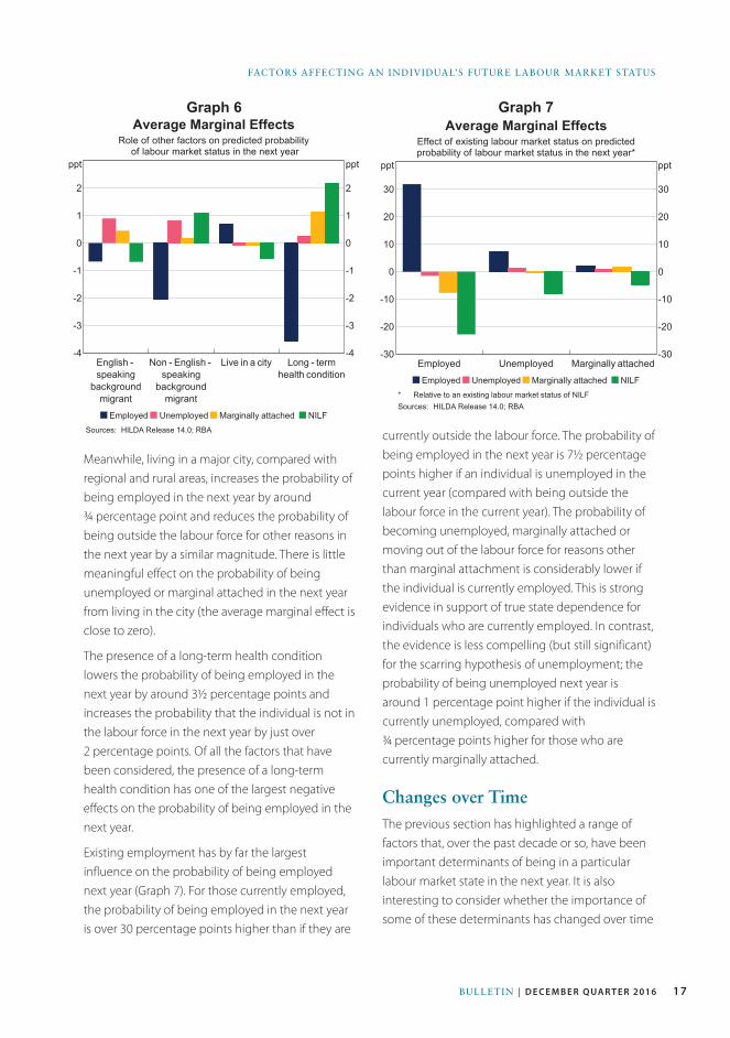
Compared with being born in Australia, being a migrant from a non-English-speaking background lowers the probability of being employed in the next year by 2 percentage points, regardless of the individual’s current labour market state, while being a migrant from an English-speaking background reduces the probability by only 0.7 percentage points (Graph 6). This supports the earlier hypothesis that migrants from a non-English-speaking background are less likely to find employment owing to potential language barriers.




currently outside the labour force. The probability of being employed in the next year is 71/2 percentage points higher if an individual is unemployed in the current year (compared with being outside the labour force in the current year). The probability of becoming unemployed, marginally attached or moving out of the labour force for reasons other than marginal attachment is considerably lower if the individual is currently employed. This is strong evidence in support of true state dependence for individuals who are currently employed. In contrast, the evidence is less compelling (but still significant) for the scarring hypothesis of unemployment; the probability of being unemployed next year is around 1 percentage point higher if the individual is currently unemployed, compared with ¾ percentage points higher for those who are currently marginally attached.

Changes over TimeThe previous section has highlighted a range of factors that, over the past decade or so, have been important determinants of being in a particular labour market state in the next year. It is also interesting to consider whether the importance of some of these determinants has changed over time

Graph 6Average Marginal Effects

Role of other factors on predicted probabilityof labour market status in the next year

English -speaking

backgroundmigrant

Non - English -speaking

backgroundmigrant

Live in a city Long - termhealth condition

-4

-3

-2

-1

0

1

2

ppt

-4

-3

-2

-1

0

1

2

ppt

Employed Unemployed Marginally attached NILFSources: HILDA Release 14.0; RBA

Graph 7Average Marginal Effects

Effect of existing labour market status on predictedprobability of labour market status in the next year*

Employed Unemployed Marginally attached-30

-20

-10

0

10

20

30

ppt

-30

-20

-10

0

10

20

30

ppt

Employed Unemployed Marginally attached NILF* Relative to an existing labour market status of NILFSources: HILDA Release 14.0; RBA

Meanwhile, living in a major city, compared with regional and rural areas, increases the probability of being employed in the next year by around ¾ percentage point and reduces the probability of being outside the labour force for other reasons in the next year by a similar magnitude. There is little meaningful effect on the probability of being unemployed or marginal attached in the next year from living in the city (the average marginal effect is close to zero).

The presence of a long-term health condition lowers the probability of being employed in the next year by around 31/2 percentage points and increases the probability that the individual is not in the labour force in the next year by just over 2 percentage points. Of all the factors that have been considered, the presence of a long-term health condition has one of the largest negative effects on the probability of being employed in the next year.

Existing employment has by far the largest influence on the probability of being employed next year (Graph 7). For those currently employed, the probability of being employed in the next year is over 30 percentage points higher than if they are




Graph 8Average Marginal Effects – Female*

Effect on predicted probability of labour marketstatus in the next period

-1.4

-0.7

0.0

0.7

1.4

ppt

Employed Unemployed Marginallyattached

-1.4

-0.7

0.0

0.7

1.4

ppt

NILF

2001–06 2007–10 2011–14 Full sample* Relative to being maleSources: HILDA Release 14.0; RBA

given the observed changes in the features of the labour market (such as the increased participation by females and older cohorts of Australians).

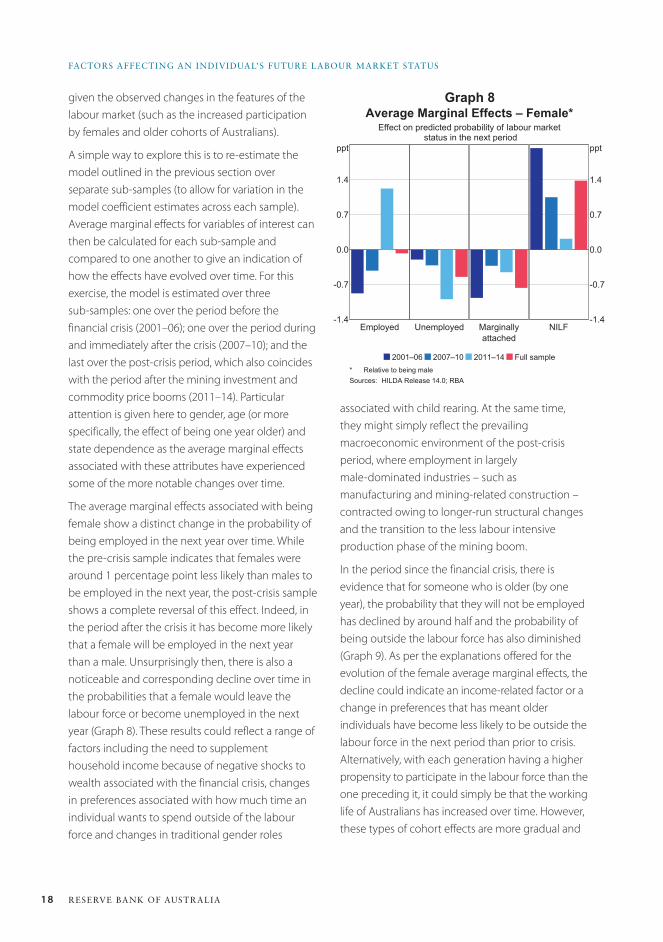
A simple way to explore this is to re-estimate the model outlined in the previous section over separate sub-samples (to allow for variation in the model coefficient estimates across each sample). Average marginal effects for variables of interest can then be calculated for each sub-sample and compared to one another to give an indication of how the effects have evolved over time. For this exercise, the model is estimated over three sub-samples: one over the period before the financial crisis (2001–06); one over the period during and immediately after the crisis (2007–10); and the last over the post-crisis period, which also coincides with the period after the mining investment and commodity price booms (2011–14). Particular attention is given here to gender, age (or more specifically, the effect of being one year older) and state dependence as the average marginal effects associated with these attributes have experienced some of the more notable changes over time.

The average marginal effects associated with being female show a distinct change in the probability of being employed in the next year over time. While the pre-crisis sample indicates that females were around 1 percentage point less likely than males to be employed in the next year, the post-crisis sample shows a complete reversal of this effect. Indeed, in the period after the crisis it has become more likely that a female will be employed in the next year than a male. Unsurprisingly then, there is also a noticeable and corresponding decline over time in the probabilities that a female would leave the labour force or become unemployed in the next year (Graph 8). These results could reflect a range of factors including the need to supplement household income because of negative shocks to wealth associated with the financial crisis, changes in preferences associated with how much time an individual wants to spend outside of the labour force and changes in traditional gender roles

associated with child rearing. At the same time, they might simply reflect the prevailing macroeconomic environment of the post-crisis period, where employment in largely male-dominated industries – such as manufacturing and mining-related construction – contracted owing to longer-run structural changes and the transition to the less labour intensive production phase of the mining boom.

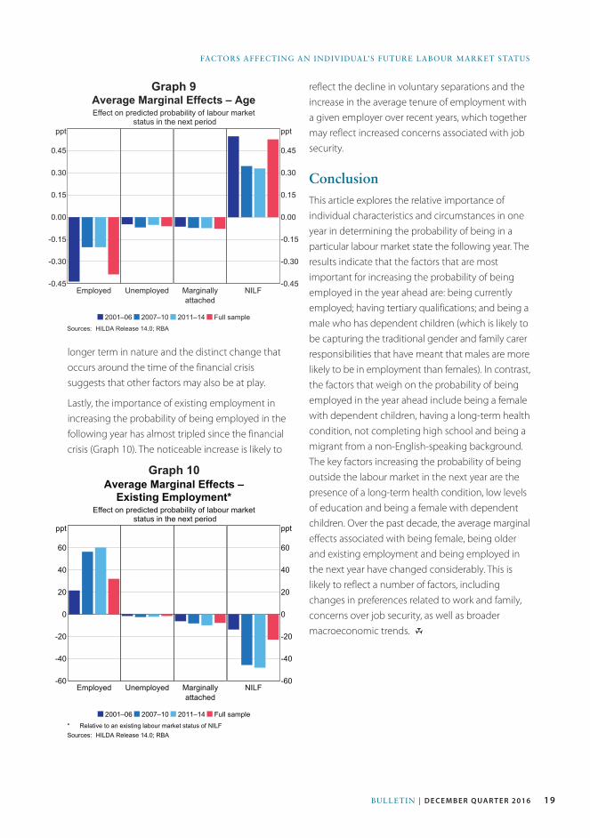
In the period since the financial crisis, there is evidence that for someone who is older (by one year), the probability that they will not be employed has declined by around half and the probability of being outside the labour force has also diminished (Graph 9). As per the explanations offered for the evolution of the female average marginal effects, the decline could indicate an income-related factor or a change in preferences that has meant older individuals have become less likely to be outside the labour force in the next period than prior to crisis. Alternatively, with each generation having a higher propensity to participate in the labour force than the one preceding it, it could simply be that the working life of Australians has increased over time. However, these types of cohort effects are more gradual and




Average Marginal Effects – AgeEffect on predicted probability of labour market

status in the next period

-0.45

-0.30

-0.15

0.00

0.15

0.30

0.45

ppt


-0.45

-0.30

-0.15

0.00

0.15

0.30

0.45

ppt

NILF

2001–06 2007–10 2011–14 Full sampleSources: HILDA Release 14.0; RBA

Graph 9

Graph 10Average Marginal Effects –

Existing Employment*Effect on predicted probability of labour market

status in the next period

-60

-40

-20

0

20

40

60

ppt


-60

-40

-20

0

20

40

60

ppt

NILF

2001–06 2007–10 2011–14 Full sample* Relative to an existing labour market status of NILFSources: HILDA Release 14.0; RBA

reflect the decline in voluntary separations and the increase in the average tenure of employment with a given employer over recent years, which together may reflect increased concerns associated with job security.

ConclusionThis article explores the relative importance of individual characteristics and circumstances in one year in determining the probability of being in a particular labour market state the following year. The results indicate that the factors that are most important for increasing the probability of being employed in the year ahead are: being currently employed; having tertiary qualifications; and being a male who has dependent children (which is likely to be capturing the traditional gender and family carer responsibilities that have meant that males are more likely to be in employment than females). In contrast, the factors that weigh on the probability of being employed in the year ahead include being a female with dependent children, having a long-term health condition, not completing high school and being a migrant from a non-English-speaking background. The key factors increasing the probability of being outside the labour market in the next year are the presence of a long-term health condition, low levels of education and being a female with dependent children. Over the past decade, the average marginal effects associated with being female, being older and existing employment and being employed in the next year have changed considerably. This is likely to reflect a number of factors, including changes in preferences related to work and family, concerns over job security, as well as broader macroeconomic trends. R

longer term in nature and the distinct change that occurs around the time of the financial crisis suggests that other factors may also be at play.

Lastly, the importance of existing employment in increasing the probability of being employed in the following year has almost tripled since the financial crisis (Graph 10). The noticeable increase is likely to




Appendix A: The Mixed Logit ModelThe mixed logit model has economic foundations in random utility theory, where there is an unobservable latent variable (here denoted by Yi ,t+1

∗ ) that represents the propensity that the observed outcome variable (here denoted by Yi ,t+1) will be equal to one for a given labour market state in the next period.

Recall, Equation (1) describes the probability that individual i will be in labour force state j in period t + 1 given their individual characteristics and circumstances in period t.

(1)

Where j = 1 refers to employed, 2 refers to unemployed, 3 refers to marginally attached and 4 refers to outside of the labour force for reasons other than marginal attachment. Xi,t is a vector of exogenous explanatory variables of observable individual characteristics in period t and Yi,t is the labour market status of individual i in period t.

The mixed logit model estimates the latent propensity that individual i will be in labour force state j in period t + 1 given their individual characteristics and circumstances in period t (Equation A1).

(A1)

Pr Yi ,t+1= j X i ,t ,Yi ,t ,Yi ,1( )=exp ′Xi ,tβ j+ ′Yi ,tγ j+ ′Yi ,1θ j( )

exp′Xi ,tβk+ ′Yi ,tγk+ ′Yi ,1θk

⎛

⎝⎜⎜⎜⎜

⎞

⎠

⎟⎟⎟⎟⎟k=1

4∑j=1,2,3,4

Yi ,t+1∗ =αi ,2d2+αi ,3d3+αi ,4d4+β j X i ,t+γ jYi ,t+θ jYi ,1+εi , j ,t+1

In addition to the variables outlined in the body of the article, dj are the alternative-specific constants (capturing the four alternative labour market states in period t + 1) which have random coefficients αi , j =α j+µi, where:

(A2)

For identification purposes αi , j =α j+µi,1d1 is normalised to zero, making employed in period t + 1 the base case. By allowing the alternative-specific coefficients to be random, potential correlation in the composite error terms is enabled as well as heteroskedasticity across the outcomes. The error term

Yi ,t+1∗ =αi ,2d2+αi ,3d3+αi ,4d4+β j X i ,t+γ jYi ,t+θ jYi ,1+εi , j ,t+1 is an

unobserved random term that is independent and identically distributed and is distributed according to the extreme value distribution.

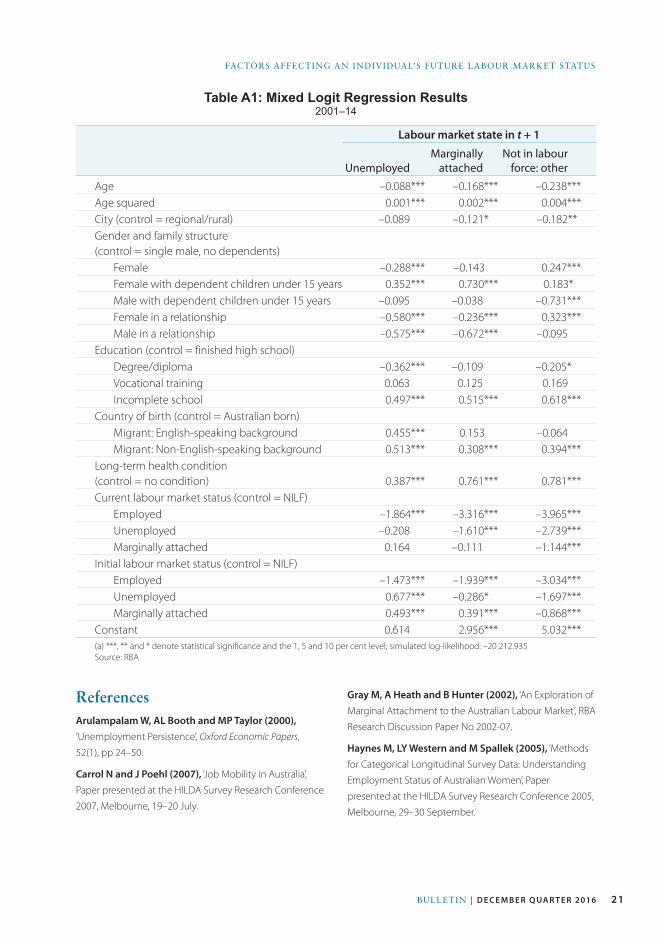
Table A1 shows the estimated coefficients from the mixed logit estimation with 250 Halton draws. The table only shows three sets of coefficient estimates because one labour market state had to be normalised to zero for identification purposes. The sign and statistical significance of the coefficients therefore need to be interpreted relative to the base case. For example, taking the coefficients associated with being female, compared with being employed in the next period, a female is less likely to be unemployed, but more likely to not be in the labour force in the next period, with both coefficients statistically significant at the 1 per cent level.

αi , j =α j+µi




Table A1: Mixed Logit Regression Results2001–14

Labour market state in t + 1

UnemployedMarginally

attachedNot in labour

force: other

Age –0.088*** –0.168*** –0.238***Age squared 0.001*** 0.002*** 0.004***City (control = regional/rural) –0.089 –0.121* –0.182**Gender and family structure (control = single male, no dependents)

Female –0.288*** –0.143 0.247***Female with dependent children under 15 years 0.352*** 0.730*** 0.183*Male with dependent children under 15 years –0.095 –0.038 –0.731***Female in a relationship –0.580*** –0.236*** 0.323***Male in a relationship –0.575*** –0.672*** –0.095

Education (control = finished high school) Degree/diploma –0.362*** –0.109 –0.205*Vocational training 0.063 0.125 0.169Incomplete school 0.497*** 0.515*** 0.618***

Country of birth (control = Australian born) Migrant: English-speaking background 0.455*** 0.153 –0.064Migrant: Non-English-speaking background 0.513*** 0.308*** 0.394***

Long-term health condition (control = no condition) 0.387*** 0.761*** 0.781***Current labour market status (control = NILF)

Employed –1.864*** –3.316*** –3.965***Unemployed –0.208 –1.610*** –2.739***Marginally attached 0.164 –0.111 –1.144***

Initial labour market status (control = NILF) Employed –1.473*** –1.939*** –3.034***Unemployed 0.677*** –0.286* –1.697***Marginally attached 0.493*** 0.391*** –0.868***

Constant 0.614 2.956*** 5.032***(a) ***, ** and * denote statistical significance and the 1, 5 and 10 per cent level; simulated log-likelihood: –20 212.935Source: RBA

ReferencesArulampalam W, AL Booth and MP Taylor (2000), ‘Unemployment Persistence’, Oxford Economic Papers,

52(1), pp 24–50.

Carrol N and J Poehl (2007), ‘Job Mobility in Australia’,

Paper presented at the HILDA Survey Research Conference

2007, Melbourne, 19–20 July.

Gray M, A Heath and B Hunter (2002), ‘An Exploration of

Marginal Attachment to the Australian Labour Market’, RBA

Research Discussion Paper No 2002-07.

Haynes M, LY Western and M Spallek (2005), ‘Methods

for Categorical Longitudinal Survey Data: Understanding

Employment Status of Australian Women’, Paper

presented at the HILDA Survey Research Conference 2005,

Melbourne, 29–30 September.




Heckman J (1981), ‘The Incidental Parameters Problem

and the Problem of Initial Conditions in Estimating

a Discrete Time-Discrete Data Stochastic Process’, in

CF Manski and D McFadden (eds), Structural Analysis of

Discrete Data with Econometric Applications, MIT Press,

Cambridge, pp 179–195.

McFadden D and K Train (2000), ‘Mixed MNL Models

for Discrete Response’, Journal of Applied Econometrics, 15,

pp 447–470.

Prowse V (2010), ‘Modeling Employment Dynamics with

State Dependence and Unobserved Heterogeneity’, IZA

Discussion Paper No 4889.

Warren D (2015), ‘Pathways to Retirement: Evidence

from the HILDA Survey’, Work, Aging and Retirement, 1(2),

pp 1–22.

Woolridge J (2005), ‘Simple Solutions to the Initial

Conditions Problem in Dynamic, Nonlinear Panel Data

Models with Unobserved Heterogeneity’, Journal of Applied

Econometrics, 20, pp 39–54.


Documents

Factors Affecting an Individual’s Future Labour Market … · Factors Affecting an Individual’s Future ... FACTORS AFFECTING AN INDIVIDUAL’S FUTURE LABOUR MARKET STATUS