Fast Marching Trees - Stanford Universityweb.stanford.edu/~pavone/papers/Janson.Pavone.ISRR13.pdf · Fast Marching Trees: a Fast Marching Sampling-Based Method for Optimal Motion

Fast Marching Trees: a Fast MarchingSampling-Based Method for Optimal MotionPlanning in Many Dimensions

Lucas Janson and Marco Pavone

Abstract In this paper we present a novel probabilistic sampling-based motionplanning algorithm called the Fast Marching Tree algorithm (FMT∗ ). The algo-rithm is specifically aimed at solving complex motion planning problems in high-dimensional configuration spaces. This algorithm is proven to be asymptotically op-timal and is shown to converge to an optimal solution faster than its state-of-the-artcounterparts, chiefly PRM* and RRT*. An additional advantage of FMT∗ is that itbuilds and maintains paths in a tree-like structure (especially useful for planning un-der differential constraints). The FMT∗ algorithm essentially performs a “lazy” dy-namic programming recursion on a set of probabilistically-drawn samples to grow atree of paths, which moves steadily outward in cost-to-come space. As such, thisalgorithm combines features of both single-query algorithms (chiefly RRT) andmultiple-query algorithms (chiefly PRM), and is conceptually related to the FastMarching Method for the solution of eikonal equations. As a departure from pre-vious analysis approaches that are based on the notion of almost sure convergence,the FMT∗ algorithm is analyzed under the notion of convergence in probability: theextra mathematical flexibility of this approach allows for significant algorithmicadvantages and provides convergence rate bounds – a first in the field of optimalsampling-based motion planning. Numerical experiments over a range of dimen-sions and obstacle configurations confirm our theoretical and heuristic argumentsby showing that FMT∗ , for a given execution time, returns substantially better so-lutions than either PRM* or RRT*, especially in high-dimensional configurationspaces.

Lucas JansonDepartment of Statistics, Stanford University, Stanford, CA 94305, e-mail: [email protected]

Marco PavoneDepartment of Aeronautics and Astronautics, Stanford University, Stanford, CA 94305, e-mail:[email protected]

A preliminary version of this work has been orally presented at the workshop on “Robotic Ex-ploration, Monitoring, and Information Collection: Nonparametric Modeling, Information-basedControl, and Planning under Uncertainty” at the Robotics: Science and Systems 2013 conference.This work has neither appeared elsewhere for publication, nor is under review for another refereedpublication.

1

2 Lucas Janson and Marco Pavone

1 IntroductionProbabilistic sampling-based algorithms represent a particularly successful ap-

proach to robotic motion planning problems in high-dimensional configurationspaces, which naturally arise, e.g., when controlling the motion of high degree-of-freedom robots or planning under uncertainty [19, 13]. Accordingly, the design ofrapidly converging sampling-based algorithms with sound performance guaranteeshas emerged as a central topic in robotic motion planning, and represents the mainthrust of this paper.

Specifically, the key idea behind probabilistic sampling-based algorithms is toavoid the explicit construction of the configuration space (which is prohibitivein the high-dimensional case), and instead conduct a search that probabilisticallyprobes the configuration space with a sampling scheme. This probing is enabledby a collision detection module, which the motion planning algorithm considersas a “black box” [13]. Probabilistic sampling-based algorithms can be divided be-tween multiple-query and single-query. Multiple-query algorithms construct a topo-logical graph called a roadmap, which allows a user to efficiently solve multipleinitial-state/goal-state queries. This family of algorithms includes the probabilisticroadmap algorithm (PRM) [10] and its variants, e.g., Lazy-PRM [3], dynamic PRM[7], and PRM* [9]. On the contrary, in single-query algorithms, a single initial-state/goal-state pair is given, and the algorithm must search until it finds a solution(or it may report early failure). This family of algorithms includes the rapidly explor-ing random trees algorithm (RRT) [14], the rapidly exploring dense trees algorithm(RDT) [13], and their variants, e.g., RRT* [9]. Other notable sampling-based plan-ners include expansive space trees (EST) [5, 16], sampling-based roadmap of trees(SRT) [17], rapidly-exploring roadmap (RRM) [1], and the “cross-entropy” plannerin [11]. Analysis in terms of convergence to feasible or even optimal solutions formultiple-query and single-query algorithms is provided in [5, 12, 2, 6, 9]. A centralresult is that these algorithms provide probabilistic completeness guarantees in thesense that the probability that the planner fails to return a solution, if one exists,decays to zero as the number of samples approaches infinity [2]. Recently, it hasbeen proven that both RRT* and PRM* are asymptotically optimal, i.e. the cost ofthe returned solution converges almost surely to the optimum [9]. Building upon theresults in [9], the work in [15] presents an algorithm with provable “sub-optimality”guarantees, which trades “optimality” with faster computation.

Statement of Contributions: The objective of this paper is to propose and an-alyze a novel probabilistic motion planning algorithm that is asymptotically opti-mal and improves upon state-of-the-art asymptotically-optimal algorithms (namelyRRT* and PRM*) in terms of the convergence rate to the optimal solution (con-vergence rate is interpreted with respect to execution time). The algorithm, namedFast Marching Tree algorithm (FMT∗), is designed to be particularly efficient inhigh-dimensional environments cluttered with obstacles. FMT∗ essentially com-bines some of the features of multiple-query algorithms with those of single-queryalgorithms, by performing a “lazy” dynamic programming recursion on a set ofprobabilistically-drawn samples in the configuration space. As such, this algorithmcombines features of PRM and SRT (similar to RRM), and grows a tree of trajec-tories like RRT. Additionally, FMT∗ is conceptually similar to the Fast MarchingMethod, one of the main methods for the solution of stationary eikonal equations[18]. As in the Fast Marching Method, the main idea is to exploit a heapsort tech-

Fast Marching Trees for Optimal Sampling-Based Motion Planning 3

nique to systematically locate the proper sample point to update and to incrementallybuild the solution in an “outward” direction, so that one needs never backtrack overpreviously evaluated sample points. Such a Dijkstra-like one-pass property is whatmakes both the Fast Marching Method and FMT∗ particularly efficient.

The end product of the FMT∗ algorithm is a tree, which, together with the con-nection to the Fast Marching Method, gives the algorithm its name. An advantage ofFMT∗with respect to PRM* (in addition to a faster convergence rate) is the fact thatFMT∗ builds and maintains paths in a tree-like structure, which is especially usefulwhen planning under differential or integral constraints. Our simulations across 2,5, 7, and 10 dimensions, both without obstacles and with 50% obstacle coverage,show that FMT∗ substantially outperforms PRM* and RRT*.

It is important to note that in this paper we use a notion of asymptotic optimality(AO) different from the one used in [9]. In [9], AO is defined through the notion ofconvergence almost everywhere (a.e.). Explicitly, in [9], an algorithm is consideredAO if the cost of the solution it returns converges a.e. to the optimal cost as the num-ber of samples n approaches infinity. This definition is completely justified when thealgorithm is sequential in n, such as RRT∗ [9], in the sense that it requires that withprobability 1, the sequence of solutions converges to an optimal one, with the solu-tion at n+1 heavily related to that at n. However, for non-sequential algorithms suchas PRM∗ and FMT∗ , there is no connection between the solutions at n and n+ 1.Since these algorithms process all the nodes at once, the solution at n+1 is based onn+1 new nodes, sampled independently of those used in the solution at n. This mo-tivates the definition of AO used in this paper, which is that the cost of the solutionreturned by an algorithm must converge in probability to the optimal cost. Althoughmathematically convergence in probability is a weaker notion than convergence a.e.(the latter implies the former), in practice there is no distinction when an algorithmis only run on a predetermined, fixed number of nodes. In this case, all that mattersis that the probability that the cost of the solution returned by the algorithm is lessthan an ε fraction greater than the optimal cost goes to 1 as n→ ∞, for any ε > 0,which is exactly the statement of convergence in probability. Since this is a mathe-matically weaker, but practically identical condition, we sought to capitalize on theextra mathematical flexibility, and indeed find that our proof of AO for FMT∗ allowsfor an improved implementation of PRM∗ in [9], providing a speed-up linear in thenumber of dimensions. Our proof of AO also gives a convergence rate bound bothfor FMT∗ and PRM* – a first in the field of optimal sampling-based motion plan-ning. Hence, an additional important contribution of this paper is the analysis of AOunder the notion of convergence in probability, which is of independent interest andcould enable the design and analysis of other AO sampling-based algorithms.

Organization: This paper is structured as follows. In Section 2 we formally de-fine the optimal path planning problem. In Section 3 we present FMT∗, and weprove some basic properties, e.g., termination. In Section 4 we prove the asymptoticoptimality of FMT∗ . In Section 5 we first conceptually discuss the advantages ofFMT∗ and then we present results from numerical experiments supporting our state-ments. Finally, in Section 6, we draw some conclusions and we discuss directionsfor future work.

Notation: Consider the Euclidean space in d dimensions, i.e., Rd . Given a pointx∈R, a ball of radius r > 0 centered at x∈Rd is defined as B(x; r) := {x∈Rd |‖x−x‖ < r}. Given a subset X of Rd , its boundary is denoted by ∂X . Given two


points x and z in Rd , the line connecting them is denoted by xz. Let ζd denote thevolume of the unit ball in the d-dimensional Euclidean space. The cardinality ofa set S is written cardS. Given a set X ⊆ Rd , µ(X ) denotes its d-dimensionalLebesgue measure. In this paper, we will interchangeably refer to points in X asnodes, samples, or vertices.

2 Problem setupThe problem formulation follows closely the problem formulation in [9]. Let

X = [0, 1]d be the configuration space, where d ∈N, d≥ 2. Let Xobs be the obstacleregion, such that X \Xobs is an open set (we consider ∂X ⊂Xobs), and denote theobstacle-free space as Xfree = cl(X \Xobs), where cl(·) denotes the closure of a set.The initial condition xinit is an element of Xfree, and the goal region Xgoal is an opensubset of Xfree. A path planning problem is denoted by a triplet (Xfree,xinit,Xgoal).A function of bounded variation σ : [0,1]→ Rd is called a path if it is continuous.A path is said to be collision-free if σ(τ) ∈Xfree for all τ ∈ [0, 1]. A path is said tobe a feasible path for the planning problem (Xfree,xinit,Xgoal) if it is collision-free,σ(0) = xinit, and σ(1) ∈ cl(Xgoal).

A goal region Xgoal is said to be regular if there exists ξ > 0 such that ∀y ∈∂Xgoal, there exists z∈Xgoal with B(z;ξ )⊆Xgoal and y∈ ∂B(z;ξ ). In other words,a regular goal region is a “well-behaved” set where the boundary has bounded cur-vature. We will say Xgoal is ξ -regular if Xgoal is regular for the parameter ξ . Let Σ

be the set of all paths. A cost function for the planning problem (Xfree,xinit,Xgoal)is a function c : Σ → R≥0 from the set of paths to the nonnegative real numbers; inthis paper we will consider as cost functions c(σ) the arc length of σ with respectto the Euclidean metric in X (recall that σ is, by definition, rectifiable). Extensionto more general cost functions (possibly not satisfying the triangle inequality) arepossible and are deferred to future work. The optimal path planning problem is thendefined as follows:

Optimal path planning problem: Given a path planning problem(Xfree,xinit,Xgoal) with a regular goal region and an arc length functionc : Σ → R≥0, find a feasible path σ∗ such that c(σ∗) = min{c(σ) :σ is feasible}. If no such path exists, report failure.

Finally, we introduce some definitions concerning the clearance of a path, i.e.,its “distance” from Xobs [9]. For a given δ > 0, the δ -interior of Xfree is definedas the set of all states that are at least a distance δ away from any point in Xobs. Acollision-free path σ is said to have strong δ -clearance if it lies entirely inside theδ -interior of Xfree. A collision-free path σ is said to have weak δ -clearance if thereexists a path σ ′ that has strong δ -clearance and there exists a homotopy ψ , withψ(0) = σ , ψ(1) = σ ′, and for all α ∈ (0,1] there exists δα > 0 such that ψ(α) hasstrong δα -clearance.

3 The Fast Marching Tree algorithm (FMT∗ )In this section we present the Fast Marching Tree algorithm, FMT∗, described in

pseudocode in Algorithm 1. We first introduce the algorithm, then discuss its ter-mination properties, and finally discuss implementation details and computationalcomplexity. The proof of its (asymptotic) optimality will be presented in Section 4.


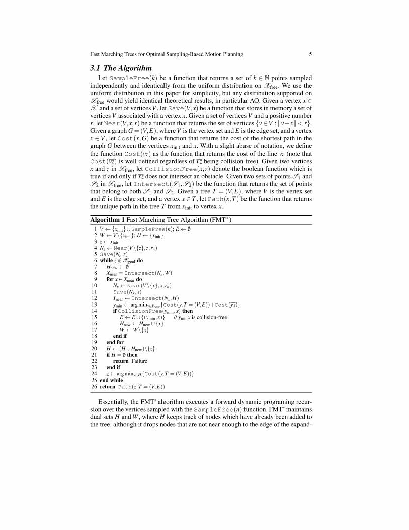
3.1 The AlgorithmLet SampleFree(k) be a function that returns a set of k ∈ N points sampled

independently and identically from the uniform distribution on Xfree. We use theuniform distribution in this paper for simplicity, but any distribution supported onXfree would yield identical theoretical results, in particular AO. Given a vertex x ∈X and a set of vertices V , let Save(V,x) be a function that stores in memory a set ofvertices V associated with a vertex x. Given a set of vertices V and a positive numberr, let Near(V,x,r) be a function that returns the set of vertices {v∈V : ‖v−x‖< r}.Given a graph G=(V,E), where V is the vertex set and E is the edge set, and a vertexx ∈ V , let Cost(x,G) be a function that returns the cost of the shortest path in thegraph G between the vertices xinit and x. With a slight abuse of notation, we definethe function Cost(vz) as the function that returns the cost of the line vz (note thatCost(vz) is well defined regardless of vz being collision free). Given two verticesx and z in Xfree, let CollisionFree(x,z) denote the boolean function which istrue if and only if xz does not intersect an obstacle. Given two sets of points S1 andS2 in Xfree, let Intersect(S1,S2) be the function that returns the set of pointsthat belong to both S1 and S2. Given a tree T = (V,E), where V is the vertex setand E is the edge set, and a vertex x ∈ T , let Path(x,T ) be the function that returnsthe unique path in the tree T from xinit to vertex x.

Algorithm 1 Fast Marching Tree Algorithm (FMT∗ )1 V ←{xinit}∪SampleFree(n); E← /02 W ←V\{xinit}; H←{xinit}3 z← xinit4 Nz← Near(V\{z},z,rn)5 Save(Nz,z)6 while z /∈Xgoal do7 Hnew← /08 Xnear = Intersect(Nz,W )9 for x ∈ Xnear do

10 Nx← Near(V\{x},x,rn)11 Save(Nx,x)12 Ynear← Intersect(Nx,H)13 ymin← argminy∈Ynear{Cost(y,T = (V,E))+Cost(yx)}14 if CollisionFree(ymin,x) then15 E← E ∪{(ymin,x)} // yminx is collision-free16 Hnew← Hnew∪{x}17 W ←W\{x}18 end if19 end for20 H← (H ∪Hnew)\{z}21 if H = /0 then22 return Failure23 end if24 z← argminy∈H{Cost(y,T = (V,E))}25 end while26 return Path(z,T = (V,E))

Essentially, the FMT∗ algorithm executes a forward dynamic programing recur-sion over the vertices sampled with the SampleFree(n) function. FMT∗maintainsdual sets H and W , where H keeps track of nodes which have already been added tothe tree, although it drops nodes that are not near enough to the edge of the expand-


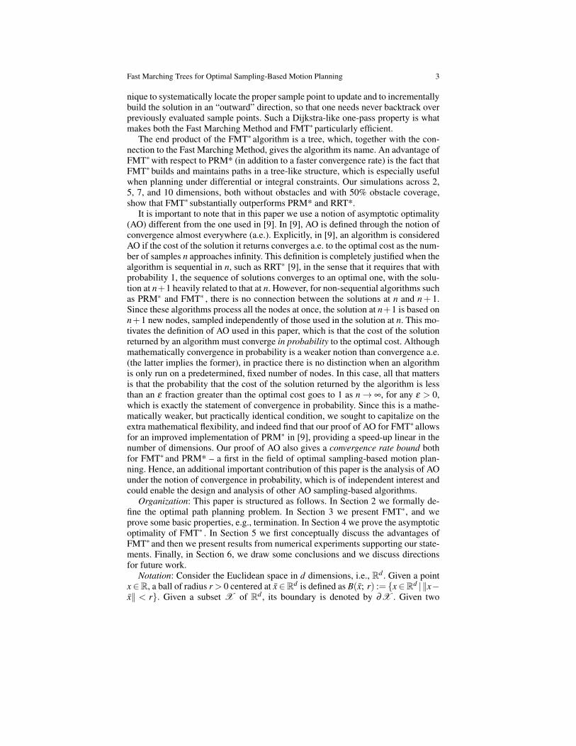
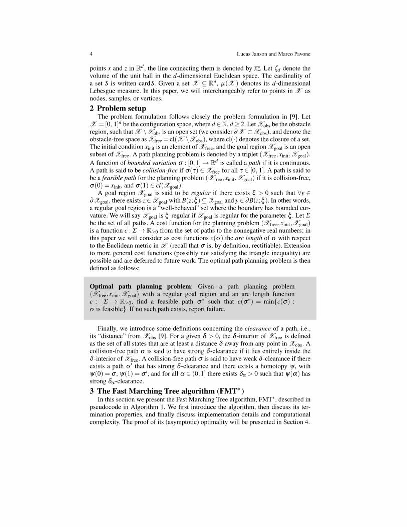
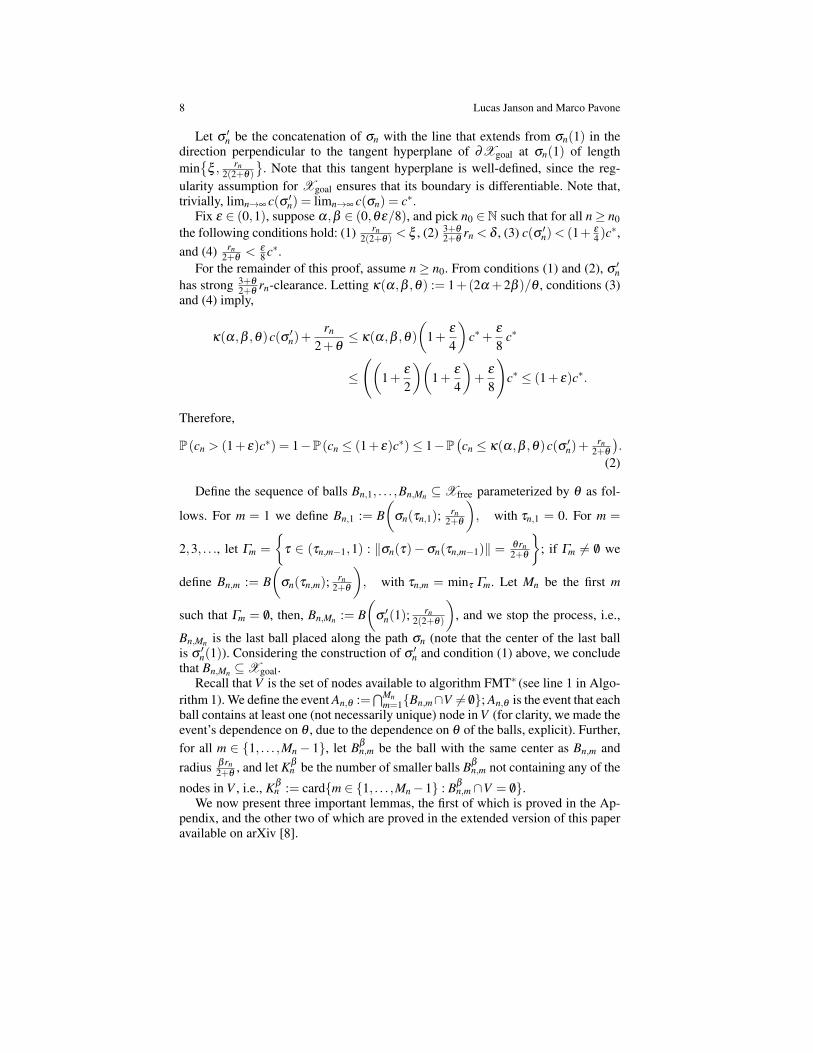
ing tree to actually have any new connections made. The set W maintains the nodeswhich have not been added to the tree. The algorithm generates a tree by movingsteadily outward in cost-to-come space (see Figure 1). To give some intuition, whenthere are no obstacles and the cost is Euclidean distance, FMT∗ reports the exactsame solution (or failure) as PRM∗. This is because, without obstacles, FMT∗ is in-deed using dynamic programming to build the minimum-cost spanning tree, withxinit as the root, of the set of nodes in the PRM∗ graph which are connected to xinit.The only difference is that by not starting with the entire PRM∗ graph itself, FMT∗ isable to find the solution much faster (see Section 5). In the presence of obstacles,FMT∗ and PRM∗ no longer return the same solution in general, and this is due tohow FMT∗ deals with obstructing obstacles. In particular, when FMT∗ searches fora connection for a node v, it will leave v unconnected (and let it remain in W to bechecked again in later iterations) if the node x ∈ H whose connection (if obstacle-free) would produce the smallest cost-to-come for v is blocked from connecting tov by an obstacle. Assuming x0 is the optimal parent of v with respect to the PRM∗graph, v will never be connected to x0 in FMT∗ only if when x0 is the minimum-costnode in H, there is another node x1 ∈ H such that (a) x1 has (necessarily, by thestructure of H) greater cost-to-come than x0, (b) x1 is within a radius rn of v, (c)x1 is blocked from connecting to v by an obstacle, and (d) obstacle-free connectionof v to x1 would have lower cost-to-come than connection to x0. If any of theseconditions fail, then on some iteration (possibly not the first), v will be connectedoptimally with respect to PRM∗. Note that the combination of conditions (a), (b),(c), and (d) ought to make such suboptimal connections quite rare.

Fig. 1 The FMT∗ algorithm generates a tree by moving steadily outward in cost-to-come space.This figure portrays the growth of the tree in a 2D environment with 1,000 nodes (not shown).

3.2 TerminationOne might wonder if, in the first place, the FMT∗ algorithm always terminates,

i.e., it does not cycle indefinitely through the sets H and W . The following theoremshows that indeed FMT∗ always terminates.

Theorem 1 (Termination). Consider a path planning problem (Xfree,xinit,Xgoal)and any n ∈N. The FMT∗ algorithm always terminates in at most n iterations of thewhile loop.

Proof. To prove that FMT∗ always terminates, note two key facts: (i) FMT∗ terminatesand reports failure if H is ever empty, and (ii) the minimum-cost node in H is re-moved from H at each while loop iteration. Therefore, to prove the theorem it suf-fices to prove the invariant that any node that has ever been added to H can neverbe added again (this, in fact, would imply that the while loop goes through at mostn iterations). To establish the invariant, observe that at a given iteration only nodes


in Xnear are added to H. However, Xnear ⊆W , so only nodes in W can be added toH, and each time a node is added, it is removed from W . Finally, since W never hasnodes added to it, a node can only be added to H once. This proves the invariant,and, in turn, the claim. ut

3.3 Implementation DetailsThe set H should be implemented as a binary min heap, ordered by cost-to-

come, with a parallel set of nodes H ′ which exactly tracks the nodes in H (but in noparticular order) for use when the intersection operation in line 12 of the algorithmis executed. For many of the nodes x ∈ V , FMT∗ saves the associated set Nx of rn-neighbors for that node. Instead of just saving a reference for each node y ∈ Nx,Nx can also have memory allocated for the real value Cost(yx) and the booleanvalue CollisionFree(y,x). Saving both of these values whenever they are firstcomputed guarantees that FMT∗will never compute them more than once for a givenpair of nodes. Finally, the first Cost function (the one that takes in a vertex andgraph) should not be a computation; the costs should just be saved for every nodethat is added to the tree. Since the cost is only queried for nodes that are already inthe tree, and that cost never changes, it would suffice to just add a step which savesthe cost-to-come of x.

Previous work has often characterized the computational complexity of an al-gorithm by how long it takes to run the algorithm on n nodes. However the com-putational complexity that ultimately matters is how long it takes for an algorithmto return a solution of a certain quality. We focus on this concept of computationalcomplexity and rely on simulations as a guide, although we note here that FMT∗ isO(n log(n)), with the proof omitted due to space limitations. In order to computethis more relevant computational complexity, we would need a characterization ofhow fast the solution improves with the number of nodes – more on this in Remark2 at the end of the next section.

4 Asymptotic Optimality of FMT∗The following theorem presents the main result of this paper.

Theorem 2 (Asymptotic optimality of FMT∗ ). Let (Xfree,xinit,Xgoal) be a pathplanning problem in d dimensions, with Xgoal ξ -regular, such that there exists anoptimal path σ∗ with weak δ -clearance for some δ > 0. Let c∗ denote the arc lengthof σ∗, and let cn denote the cost of the path returned by FMT∗ (or ∞ if FMT∗ returnsfailure) with n vertices using the following radius,

rn = (1+η) ·2(

1d

) 1d(

µ(Xfree)

ζd

) 1d(

log(n)n

) 1d, (1)

for some η > 0. Then limn→∞ P(cn > (1+ ε)c∗) = 0 for all ε > 0.

Proof. Note that c∗ = 0 implies xinit ∈ cl(Xgoal), and the result is trivial, there-fore assume c∗ > 0. Fix θ ∈ (0,1/4) and define the sequence of paths σn such thatlimn→∞ c(σn) = c∗, σn(1) ∈ ∂Xgoal, σn(τ) /∈Xgoal for all τ ∈ (0,1), σn(0) = xinit,and σn has strong δn-clearance, where δn = min

{δ , 3+θ

2+θrn}

. A proof that such asequence of paths exists can be found in [9] as Lemma 50. It requires a slew of extranotation and metric space results, and so the proof is omitted here.


Let σ ′n be the concatenation of σn with the line that extends from σn(1) in thedirection perpendicular to the tangent hyperplane of ∂Xgoal at σn(1) of lengthmin{

ξ , rn2(2+θ)

}. Note that this tangent hyperplane is well-defined, since the reg-

ularity assumption for Xgoal ensures that its boundary is differentiable. Note that,trivially, limn→∞ c(σ ′n) = limn→∞ c(σn) = c∗.

Fix ε ∈ (0,1), suppose α,β ∈ (0,θε/8), and pick n0 ∈N such that for all n≥ n0the following conditions hold: (1) rn

2(2+θ) < ξ , (2) 3+θ

2+θrn < δ , (3) c(σ ′n)< (1+ ε

4 )c∗,

and (4) rn2+θ

< ε

8 c∗.For the remainder of this proof, assume n≥ n0. From conditions (1) and (2), σ ′n

has strong 3+θ

2+θrn-clearance. Letting κ(α,β ,θ) := 1+(2α +2β )/θ , conditions (3)

and (4) imply,

κ(α,β ,θ)c(σ ′n)+rn

2+θ≤ κ(α,β ,θ)

(1+

ε

4

)c∗+

ε

8c∗

≤

((1+

ε

2

)(1+

ε

4

)+

ε

8

)c∗ ≤ (1+ ε)c∗.

Therefore,

P(cn > (1+ ε)c∗) = 1−P(cn ≤ (1+ ε)c∗)≤ 1−P(cn ≤ κ(α,β ,θ)c(σ ′n)+

rn2+θ

).

(2)

Define the sequence of balls Bn,1, . . . ,Bn,Mn ⊆Xfree parameterized by θ as fol-

lows. For m = 1 we define Bn,1 := B(

σn(τn,1); rn2+θ

), with τn,1 = 0. For m =

2,3, . . ., let Γm =

{τ ∈ (τn,m−1,1) : ‖σn(τ)−σn(τn,m−1)‖ = θrn

2+θ

}; if Γm 6= /0 we

define Bn,m := B(

σn(τn,m); rn2+θ

), with τn,m = minτ Γm. Let Mn be the first m

such that Γm = /0, then, Bn,Mn := B(

σ ′n(1);rn

2(2+θ)

), and we stop the process, i.e.,

Bn,Mn is the last ball placed along the path σn (note that the center of the last ballis σ ′n(1)). Considering the construction of σ ′n and condition (1) above, we concludethat Bn,Mn ⊆Xgoal.

Recall that V is the set of nodes available to algorithm FMT∗ (see line 1 in Algo-rithm 1). We define the event An,θ :=

⋂Mnm=1{Bn,m∩V 6= /0}; An,θ is the event that each

ball contains at least one (not necessarily unique) node in V (for clarity, we made theevent’s dependence on θ , due to the dependence on θ of the balls, explicit). Further,for all m ∈ {1, . . . ,Mn− 1}, let Bβ

n,m be the ball with the same center as Bn,m andradius β rn

2+θ, and let Kβ

n be the number of smaller balls Bβn,m not containing any of the

nodes in V , i.e., Kβn := card{m ∈ {1, . . . ,Mn−1} : Bβ

n,m∩V = /0}.We now present three important lemmas, the first of which is proved in the Ap-

pendix, and the other two of which are proved in the extended version of this paperavailable on arXiv [8].


Lemma 1. Under the assumptions of Theorem 2 and assuming n≥ n0, the followinginequality holds:

P(cn ≤ κ(α,β ,θ)c(σ ′n)+

rn2+θ

)≥ 1 − P(Kβ

n ≥ α(Mn−1))−P(Acn,θ ).

Lemma 2. Under the assumptions of Theorem 2, for all α ∈ (0,1) and β ∈ (0,θ/2),it holds that: limn→∞P(Kβ

n ≥ α(Mn−1)) = 0.

Lemma 3. Under the assumptions of Theorem 2, assume that rn = γ (logn/n)1/d ,where γ = (1 + η) · 2(1/d)

1d (µ(Xfree)/ζd)

1/d and η > 0. Then for all θ < 2η ,limn→∞P(Ac

n,θ ) = 0.

Essentially, Lemma 1 provides a lower bound for the cost of the solution deliv-ered by FMT∗ in terms of the probabilities that the “big” balls and “small” balls donot contain vertices in V . Lemma 2 states that the probability that the fraction ofsmall balls not containing vertices in V is larger than an α fraction of the total num-ber of balls is asymptotically zero. Finally, Lemma 3 states that the probability thatat least one “big” ball does not contain any of the vertices in V is asymptoticallyzero.

The asymptotic optimality claim of the theorem then follows easily. Let ε ∈ (0,1)and pick θ ∈ (0,min{2η ,1/4}) and α,β ∈ (0,θε/8)⊂ (0,θ/2). From equation (2)and Lemma 1, one can write

limn→∞

P(cn > (1+ ε)c∗)≤ limn→∞

P(

Kβn ≥ α(Mn−1)

)+ lim

n→∞P(

Acn,θ

).

The right hand-side of this equation equals zero by Lemmas 2 and 3, and the claimis proven. The case with general ε follows by monotonicity in ε of the above prob-ability. utRemark 1. Since the solution returned by FMT∗ is never better than the one returnedby PRM∗, the exact same result holds for PRM∗. Note that this proof uses a γ whichis a factor of (d + 1)1/d smaller (and thus a rn which is (d + 1)1/d smaller) thanthat in [9]. Since the number of cost computations and checks to collision-free scaleapproximately as rd

n , this factor should reduce run time substantially for a givennumber of nodes, especially in high dimensions. This is due to the difference indefinitions of AO mentioned earlier which, again, makes no practical difference forPRM∗ or FMT∗ . Furthermore, the result holds for PRM∗ under the more generalcost definition used in [9] under the new definition of AO by replacing Lemma 52in [9] with Lemma 3 from this paper.Remark 2. We now note a very intriguing and promising side-effect of the new def-inition of AO. In proving that P(cn > (1+ ε)c∗)→ 0 for all ε > 0, we actuallyhad to characterize this probability. Although the details of the functional form arescattered throughout the proof of Theorem 2 (much of which is presented in theextended version of this paper in [8]), a convergence rate bound for FMT∗ , and thusalso PRM*, can be obtained as a function of n. As far as the authors are aware,this would be the first such convergence rate result for an optimal sampling-basedmotion-planning algorithm, and would be an important step towards understandingthe behavior of this class of algorithms. An experimental verification of the tightnessof this bound is left for future work.


5 Numerical Experiments and DiscussionIn this section we discuss the advantages of FMT∗ over previous sampling-based

motion planning algorithms. To the best of our knowledge, the only other asymptot-ically optimal algorithms are PRM∗, RRG, and RRT∗ [9], so it is with these state-of-the-art methods that we draw comparison. We first present a conceptual comparisonbetween FMT∗ and such algorithms, and then we present results from numericalexperiments.

5.1 Conceptual Comparison with Existing AO AlgorithmsAs compared to RRT∗, we expect FMT∗ to show some improvement in solu-

tion quality per number of nodes placed. This is because for a given set of nodes,FMT∗ creates connections nearly optimally (exactly optimally when there are noobstacles) within the radius constraints, while RRT*, even with its rewiring step, isultimately a greedy algorithm. It is however hard to conceptually compare how longthe algorithms might take to run on a given set of nodes, given how differently theygenerate paths.

One advantage of FMT∗ over the graph-based methods such as PRM∗ and RRGis that FMT∗ builds paths in a tree-like structure at all times. This is important whendifferential or integral constraints are added to the paths. If, for example, a smooth-ness constraint is placed on paths, then since FMT∗ builds its paths outwards, eachnew branch solves the differentially constrained system with initial conditions start-ing from its parent node/state, whose optimal path has already been determined.In graph-based methods, many edges are added at once with no well-defined par-ent, so that it is not clear what the initial conditions are that need to be satisfiedfor each edge. Even in RRT∗, the rewiring process reroutes an already differentiallyconstrained path in the middle of the path, a more challenging problem than justconcatenating to the end.

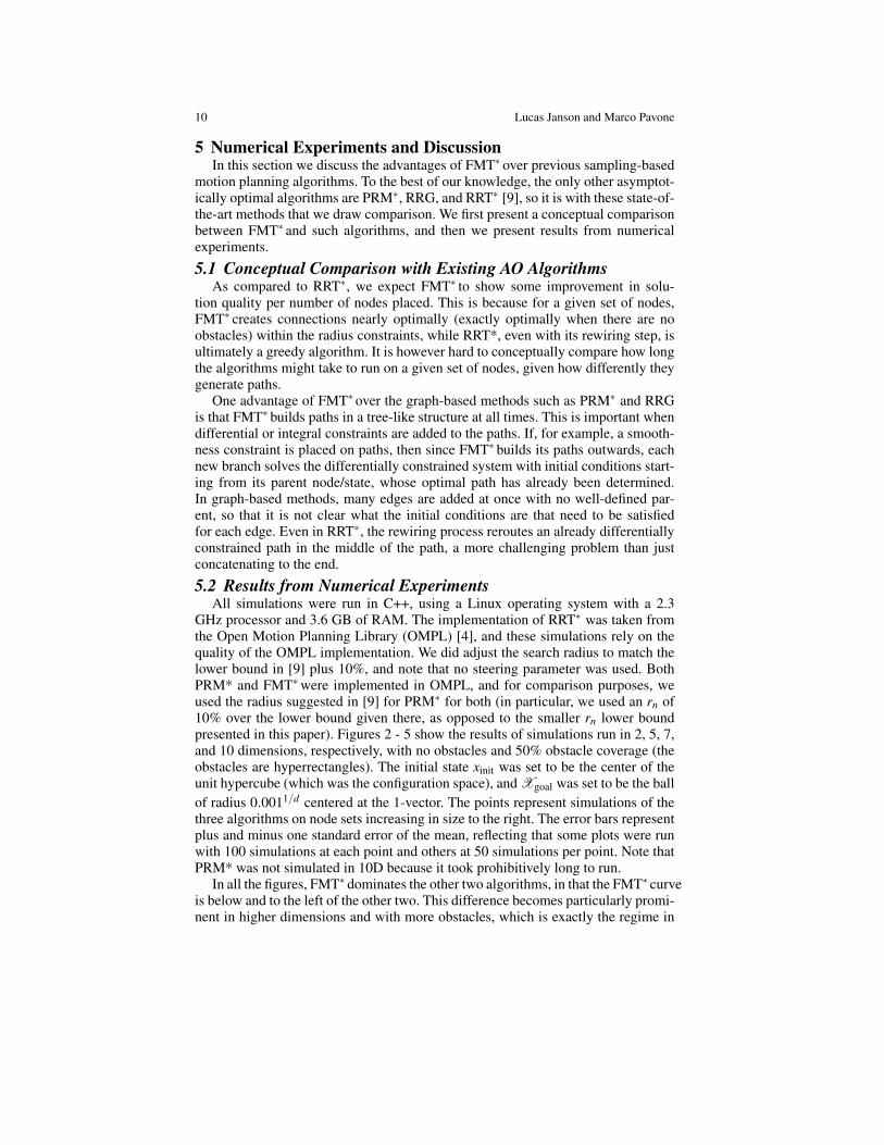
5.2 Results from Numerical ExperimentsAll simulations were run in C++, using a Linux operating system with a 2.3

GHz processor and 3.6 GB of RAM. The implementation of RRT∗ was taken fromthe Open Motion Planning Library (OMPL) [4], and these simulations rely on thequality of the OMPL implementation. We did adjust the search radius to match thelower bound in [9] plus 10%, and note that no steering parameter was used. BothPRM* and FMT∗were implemented in OMPL, and for comparison purposes, weused the radius suggested in [9] for PRM∗ for both (in particular, we used an rn of10% over the lower bound given there, as opposed to the smaller rn lower boundpresented in this paper). Figures 2 - 5 show the results of simulations run in 2, 5, 7,and 10 dimensions, respectively, with no obstacles and 50% obstacle coverage (theobstacles are hyperrectangles). The initial state xinit was set to be the center of theunit hypercube (which was the configuration space), and Xgoal was set to be the ballof radius 0.0011/d centered at the 1-vector. The points represent simulations of thethree algorithms on node sets increasing in size to the right. The error bars representplus and minus one standard error of the mean, reflecting that some plots were runwith 100 simulations at each point and others at 50 simulations per point. Note thatPRM* was not simulated in 10D because it took prohibitively long to run.

In all the figures, FMT∗ dominates the other two algorithms, in that the FMT∗ curveis below and to the left of the other two. This difference becomes particularly promi-nent in higher dimensions and with more obstacles, which is exactly the regime in


0 0.2 0.4 0.6 0.8 11

1.005

1.01

1.015

Average Execution Time [s]

Av

era

ge

Co

st,

No

rma

lize

d

2D with 0% Obstacle Coverage

FMT*

RRT*

PRM*

0 0.5 1 1.5 20.75

0.8

0.85

0.9

0.95


Av

era

ge

Co

st


FMT*

RRT*

PRM*

Fig. 2 Simulation results in 2 dimensions with and without obstacles. Left figure: (normalized)cost versus time with 0% obstacle coverage. Right figure: cost versus time with 50% obstaclecoverage.

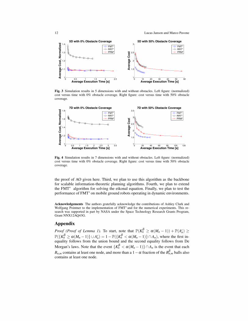
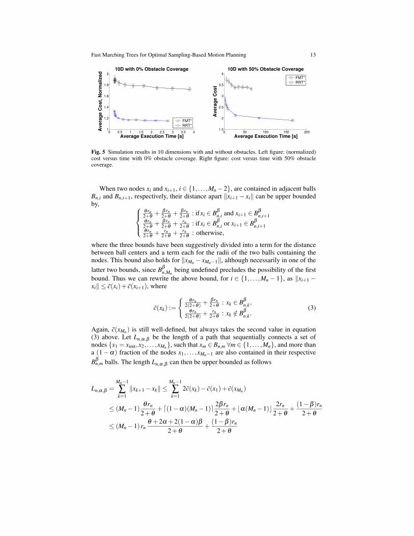
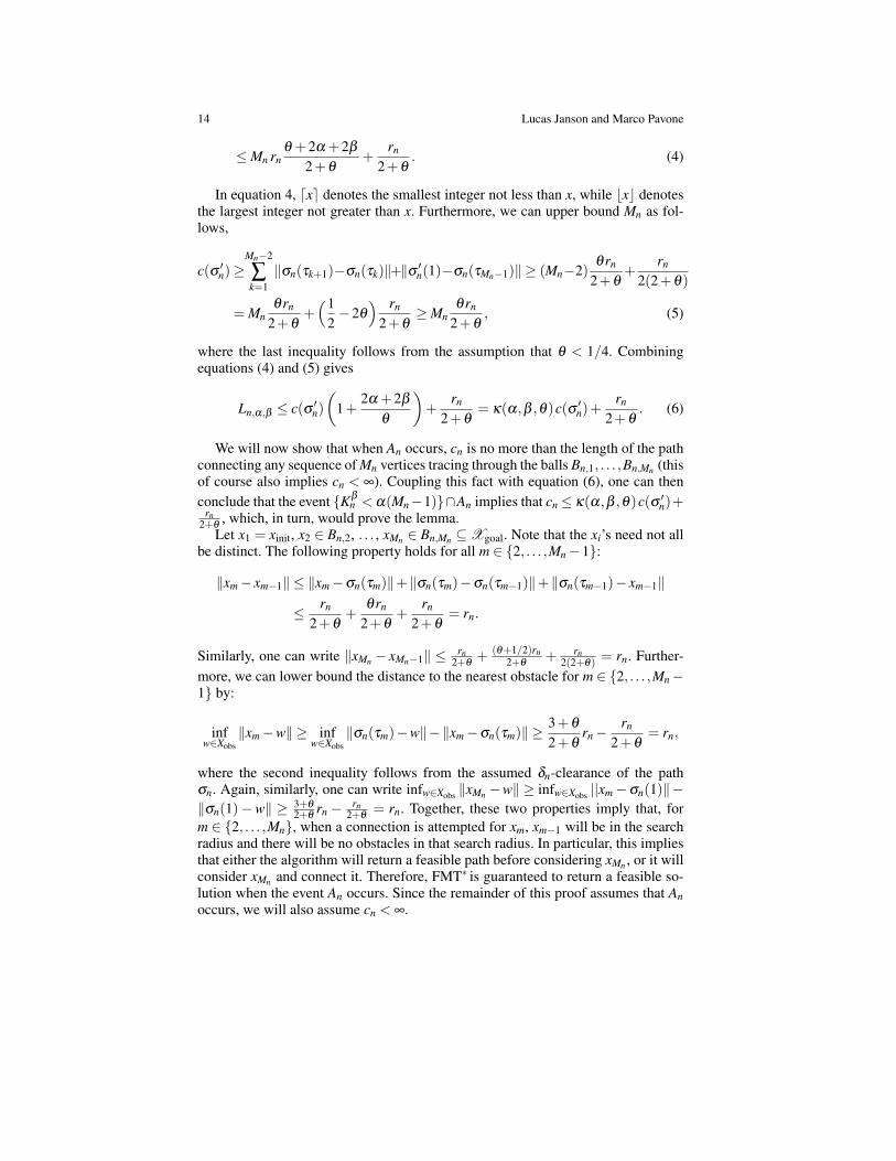
which sampling-based motion planning algorithms are particularly useful. Specifi-cally, note that in Figures 4 and 5, the solution of RRT* never even dips below thesolution of FMT∗ on the smallest node set, making it hard to estimate the speedup,but it is clearly multiple orders of magnitude. As compared to PRM*, FMT∗ still pro-vides substantial speedups in the plots with 50% obstacle coverage, and even in the0% obstacles plots for 5D and 7D, while both curves seem to plateau, FMT∗ reachesthat plateau in about half the time of PRM*.

We also note that, although it is not exactly clear from these plots because thepoints are not labeled with the number of nodes, when all three algorithms are runon the same number of nodes, the curve for PRM* looks very much like that forFMT∗ but shifted to the right (same solution quality, but slower), while that of RRT*looks very much like that of FMT∗ but shifted up (lower solution quality in the sameamount of time). This agrees with our heuristic analysis. It is of some interest tonote that in 10D with 50% obstacle coverage, RRT* only returned a solution about90% of the time across the number of nodes simulated, while FMT∗ had a 100%success rate for all but the smallest two node sets (200 nodes = 94%, 300 nodes =96%). Finally, although the error bars depend on the number of simulations, eachgraph used the same number of simulations for each point, and thus it is noteworthythat RRT*’s error bars are uniformly larger than those of FMT∗ . This means thatthe solutions returned by FMT∗ are both higher quality and more consistent.

6 ConclusionsIn this paper we have introduced and analyzed a novel probabilistic sampling-

based motion planning algorithm called Fast Marching Tree algorithm (FMT∗). Thisalgorithm is asymptotically optimal and appears to converge significantly faster thenits state-of-the-art counterparts. We used the weaker notion of convergence in prob-ability, as opposed to convergence almost surely, and showed that the extra mathe-matical flexibility provides substantial theoretical and algorithmic benefits, includ-ing convergence rate bounds.

This paper leaves numerous important extensions open for further research. First,it is of interest to extend the FMT∗ algorithm to address problems with differen-tial motion constraints and in non-metric spaces (relevant, e.g., for information-planning). Second, we plan to explore the convergence rate bounds provided by


0 0.5 1 1.5 2 2.51

1.1

1.2

1.3

1.4


Av

era

ge

Co

st,

No

rma

lize

d


FMT*

RRT*

PRM*

0 10 20 30 40 50 601

1.5

2

2.5

3


Av

era

ge

Co

st


FMT*

RRT*

PRM*


0 0.5 1 1.5 2 2.5 3 3.51

1.2

1.4

1.6

1.8


Av

era

ge

Co

st,

No

rma

lize

d


FMT*

RRT*

PRM*

0 20 40 60 80 100 1201

1.5

2

2.5

3

3.5


Av

era

ge

Co

st


FMT*

RRT*

PRM*


the proof of AO given here. Third, we plan to use this algorithm as the backbonefor scalable information-theoretic planning algorithms. Fourth, we plan to extendthe FMT∗ algorithm for solving the eikonal equation. Finally, we plan to test theperformance of FMT∗ on mobile ground robots operating in dynamic environments.

Acknowledgements The authors gratefully acknowledge the contributions of Ashley Clark andWolfgang Pointner to the implementation of FMT∗ and for the numerical experiments. This re-search was supported in part by NASA under the Space Technology Research Grants Program,Grant NNX12AQ43G.

AppendixProof (Proof of Lemma 1). To start, note that P(Kβ

n ≥ α(Mn − 1)) + P(Acn) ≥

P({Kβn ≥ α(Mn− 1)}∪Ac

n) = 1−P({Kβn < α(Mn− 1)}∩An), where the first in-

equality follows from the union bound and the second equality follows from DeMorgan’s laws. Note that the event {Kβ

n < α(Mn− 1)}∩An is the event that eachBn,m contains at least one node, and more than a 1−α fraction of the Bβ

n,m balls alsocontains at least one node.


0 0.5 1 1.5 2 2.5 3 3.5 41

1.2

1.4

1.6

1.8

2


Av

era

ge

Co

st,

No

rma

lize

d


FMT*

RRT*

0 50 100 150 2001.5

2

2.5

3

3.5

4


Av

era

ge

Co

st


FMT*

RRT*


When two nodes xi and xi+1, i ∈ {1, . . . ,Mn−2}, are contained in adjacent ballsBn,i and Bn,i+1, respectively, their distance apart ‖xi+1− xi‖ can be upper boundedby,

θrn2+θ

+ β rn2+θ

+ β rn2+θ

: ifxi ∈ Bβ

n,i and xi+1 ∈ Bβ

n,i+1θrn2+θ

+ β rn2+θ

+ rn2+θ

: ifxi ∈ Bβ

n,i or xi+1 ∈ Bβ

n,i+1θrn2+θ

+ rn2+θ

+ rn2+θ

: otherwise,

where the three bounds have been suggestively divided into a term for the distancebetween ball centers and a term each for the radii of the two balls containing thenodes. This bound also holds for ‖xMn − xMn−1‖, although necessarily in one of thelatter two bounds, since Bβ

n,Mnbeing undefined precludes the possibility of the first

bound. Thus we can rewrite the above bound, for i ∈ {1, . . . ,Mn− 1}, as ‖xi+1−xi‖ ≤ c(xi)+ c(xi+1), where

c(xk) :=

{θrn

2(2+θ) +β rn2+θ

: xk ∈ Bβ

n,k,θrn

2(2+θ) +rn

2+θ: xk /∈ Bβ

n,k.(3)

Again, c(xMn) is still well-defined, but always takes the second value in equation(3) above. Let Ln,α,β be the length of a path that sequentially connects a set ofnodes {x1 = xinit,x2, . . . ,xMn}, such that xm ∈ Bn,m ∀m ∈ {1, . . . ,Mn}, and more thana (1−α) fraction of the nodes x1, . . . ,xMn−1 are also contained in their respectiveBβ

n,m balls. The length Ln,α,β can then be upper bounded as follows

Ln,α,β =Mn−1

∑k=1‖xk+1− xk‖ ≤

Mn−1

∑k=1

2c(xk)− c(x1)+ c(xMn)

≤ (Mn−1)θrn

2+θ+ d(1−α)(Mn−1)e 2β rn

2+θ+ bα(Mn−1)c 2rn

2+θ+

(1−β )rn

2+θ

≤ (Mn−1)rnθ +2α +2(1−α)β

2+θ+

(1−β )rn

2+θ


≤Mn rnθ +2α +2β

2+θ+

rn

2+θ. (4)

In equation 4, dxe denotes the smallest integer not less than x, while bxc denotesthe largest integer not greater than x. Furthermore, we can upper bound Mn as fol-lows,

c(σ ′n)≥Mn−2

∑k=1‖σn(τk+1)−σn(τk)‖+‖σ ′n(1)−σn(τMn−1)‖ ≥ (Mn−2)

θrn

2+θ+

rn

2(2+θ)

= Mnθrn

2+θ+(1

2−2θ

) rn

2+θ≥Mn

θrn

2+θ, (5)

where the last inequality follows from the assumption that θ < 1/4. Combiningequations (4) and (5) gives

Ln,α,β ≤ c(σ ′n)(

1+2α +2β

θ

)+

rn

2+θ= κ(α,β ,θ)c(σ ′n)+

rn

2+θ. (6)

We will now show that when An occurs, cn is no more than the length of the pathconnecting any sequence of Mn vertices tracing through the balls Bn,1, . . . ,Bn,Mn (thisof course also implies cn < ∞). Coupling this fact with equation (6), one can thenconclude that the event {Kβ

n <α(Mn−1)}∩An implies that cn≤ κ(α,β ,θ)c(σ ′n)+rn

2+θ, which, in turn, would prove the lemma.

Let x1 = xinit, x2 ∈ Bn,2, . . . , xMn ∈ Bn,Mn ⊆Xgoal. Note that the xi’s need not allbe distinct. The following property holds for all m ∈ {2, . . . ,Mn−1}:

‖xm− xm−1‖ ≤ ‖xm−σn(τm)‖+‖σn(τm)−σn(τm−1)‖+‖σn(τm−1)− xm−1‖

≤ rn

2+θ+

θrn

2+θ+

rn

2+θ= rn.

Similarly, one can write ‖xMn − xMn−1‖ ≤ rn2+θ

+ (θ+1/2)rn2+θ

+ rn2(2+θ) = rn. Further-

more, we can lower bound the distance to the nearest obstacle for m ∈ {2, . . . ,Mn−1} by:

infw∈Xobs

‖xm−w‖ ≥ infw∈Xobs

‖σn(τm)−w‖−‖xm−σn(τm)‖ ≥3+θ

2+θrn−

rn

2+θ= rn,

where the second inequality follows from the assumed δn-clearance of the pathσn. Again, similarly, one can write infw∈Xobs ‖xMn −w‖ ≥ infw∈Xobs ||xm−σn(1)‖−‖σn(1)−w‖ ≥ 3+θ

2+θrn − rn

2+θ= rn. Together, these two properties imply that, for

m ∈ {2, . . . ,Mn}, when a connection is attempted for xm, xm−1 will be in the searchradius and there will be no obstacles in that search radius. In particular, this impliesthat either the algorithm will return a feasible path before considering xMn , or it willconsider xMn and connect it. Therefore, FMT∗ is guaranteed to return a feasible so-lution when the event An occurs. Since the remainder of this proof assumes that Anoccurs, we will also assume cn < ∞.


Finally, assuming xm is contained in an edge, let c(xm) denote the (unique) cost-to-come of xm in the graph generated by FMT∗ at the end of the algorithm, justbefore the path is returned. If xm is not contained in an edge, we set c(xm) = ∞.Note that c(·) is well-defined, since if xm is contained in any edge, it must be con-nected through a unique path to xinit. We claim that for all m ∈ {2, . . . ,Mn}, eithercn ≤ ∑

m−1k=1 ‖xk+1− xk‖, or c(xm)≤ ∑

m−1k=1 ‖xk+1− xk‖. In particular, taking m = Mn,

this would imply that cn ≤ min{c(xMn),∑Mn−1k=1 ‖xk+1− xk‖} ≤ ∑

Mn−1k=1 ‖xk+1− xk‖,

which, as argued before, would imply the claim.The claim is proved by induction on m. The case of m = 1 is trivial, since the

first step in the FMT∗ algorithm is to make every collision-free connection betweenxinit = x1 and the nodes contained in B(xinit;rn), which will include x2 and, thus,c(x2) = ‖x2− x1‖. Now suppose the claim is true for m−1. There are four cases toconsider:

1. cn ≤ ∑m−2k=1 ‖xk+1− xk‖,

2. c(xm−1)≤ ∑m−2k=1 ‖xk+1− xk‖ and FMT∗ ends before considering xm,

3. c(xm−1)≤ ∑m−2k=1 ‖xk+1− xk‖ and xm−1 ∈ H when xm is first considered,

4. c(xm−1)≤ ∑m−2k=1 ‖xk+1− xk‖ and xm−1 /∈ H when xm is first considered.

Case 1: cn ≤ ∑m−2k=1 ‖xk+1− xk‖ ≤ ∑

m−1k=1 ‖xk+1− xk‖, thus the claim is true for m.

Case 2: c(xm−1) < ∞ implies that xm−1 enters H at some point during FMT∗ .However, if xm−1 were ever the minimum-cost element of H, xm would have beenconsidered, and thus FMT∗must have returned a feasible solution before xm−1 wasever the minimum-cost element of H. Since the end-node of the solution returnedmust have been the minimum-cost element of H, cn ≤ c(xm−1) ≤ ∑

m−2k=1 ‖xk+1 −

xk‖ ≤ ∑m−1k=1 ‖xk+1− xk‖, thus the claim is true for m.

Case 3: xm−1 ∈H when xm is first considered, ‖xm−xm−1‖ ≤ rn, and there are noobstacles in B(xm;rn). Therefore, xm must be connected to some parent when it isfirst considered, and c(xm) ≤ c(xm−1)+‖xm− xm−1‖ ≤ ∑

m−1k=1 ‖xk+1− xk‖, thus the

claim is true for m.Case 4: When xm is first considered, there must exist z ∈ B(xm;rn) such that z is

the minimum-cost element of H, while xm−1 has not even entered H yet. Note thatagain, since B(xm;rn) intersects no obstacles and contains at least one node in H, xmmust be connected to some parent when it is first considered. Since c(xm−1) < ∞,there is a well-defined path P = {v1, . . . ,vq} from xinit = v1 to xm−1 = vq for someq ∈ N. Let w = v j, where j = maxi∈{1,...,q}{i : vi ∈ H when xm is first considered}.Then there are two subcases, either w ∈ B(xm;rn) or w /∈ B(xm;rn). If w ∈ B(xm;rn),then,

c(xm)≤ c(w)+‖xm−w‖ ≤ c(w)+‖xm−1−w‖+‖xm− xm−1‖

≤ c(xm−1)+‖xm− xm−1‖ ≤m−1

∑k=1‖xk+1− xk‖,

thus the claim is true for m (the second and third inequalities follow from the triangleinequality). If w /∈ B(xm;rn), then,


c(xm)≤ c(z)+‖xm− z‖ ≤ c(w)+ rn ≤ c(xm−1)+‖xm− xm−1‖ ≤m−1

∑k=1‖xk+1− xk‖,

where the third inequality follows from the fact that w /∈ B(xm,rn), which means thatany path through w to xm, in particular the path P ∪ xm, must traverse a distance ofat least rn between w and xm. Thus, in the final subcase of the final case, the claimis true for m.

Hence, we can conclude that cn ≤∑Mn−1k=1 ‖xk+1−xk‖. As argued before, coupling

this fact with equation (6), one can conclude that the event {Kβn < α(Mn−1)}∩An

implies that cn ≤ κ(α,β ,θ)c(σ ′n)+rn

2+θ, and the claim follows. ut

References[1] R. Alterovitz, S. Patil, and A. Derbakova. Rapidly-exploring roadmaps: Weighing explo-

ration vs. refinement in optimal motion planning. In Proc. IEEE Conf. on Robotics andAutomation, pages 3706–3712, 2011.

[2] J. Barraquand, L. Kavraki, R. Motwani, J.-C. Latombe, Tsai-Y. Li, and P. Raghavan. Arandom sampling scheme for path planning. In International Journal of Robotics Research,pages 249–264. Springer, 2000.

[3] R. Bohlin and L. E. Kavraki. Path planning using lazy PRM. In Proc. IEEE Conf. on Roboticsand Automation, volume 1, pages 521–528, 2000.

[4] I. A. Sucan, M. Moll, and L. E. Kavraki. The Open Motion Planning Library. IEEE Robotics& Automation Magazine, 19(4):72–82, December 2012. http://ompl.kavrakilab.org.

[5] D. Hsu, J. C. Latombe, and R. Motwani R. Path planning in expansive configuration spaces.International Journal of Computational Geometry & Applications, 9:495–512, 1999.

[6] D. Hsu, J.-C. Latombe, and H. Kurniawati. On the probabilistic foundations of probabilisticroadmap planning. International Journal of Robotics Research, 25(7):627–643, 2006.

[7] L. Jaillet and T. Simeon. A PRM-based motion planner for dynamically changing environ-ments. In Proc. IEEE Conf. on Robotics and Automation, volume 2, pages 1606–1611, 2004.

[8] L. Janson and M. Pavone. Fast Marching Trees: a fast marching sampling-based methodfor optimal motion planning in many dimensions – extended version. 2013. Available at:http://arxiv.org/abs/1306.3532.

[9] S. Karaman and E. Frazzoli. Sampling-based algorithms for optimal motion planning. Inter-national Journal of Robotics Research, 30(7):846–894, 2011.

[10] L.E. Kavraki, P. Svestka, J.-C. Latombe, and M.H. Overmars. Probabilistic roadmaps forpath planning in high-dimensional configuration spaces. IEEE Transactions on Robotics andAutomation, 12(4):566 –580, 1996.

[11] M. Kobilarov. Cross-entropy motion planning. International Journal of Robotics Research,31(7):855–871, 2012.

[12] A. M. Ladd and L. E. Kavraki. Measure theoretic analysis of probabilistic path planning.IEEE Transactions on Robotics and Automation, 20(2):229–242, 2004.

[13] S. Lavalle. Planning Algorithms. Cambridge University Press, 2006.[14] S. M. LaValle and J. J. Kuffner. Randomized kinodynamic planning. International Journal

of Robotics Research, 20(5):378–400, 2001.[15] J. D. Marble and K. E. Bekris. Towards small asymptotically near-optimal roadmaps. In

Proc. IEEE Conf. on Robotics and Automation, 2012.[16] J. M Phillips, N. Bedrossian, and L. E. Kavraki. Guided expansive spaces trees: A search

strategy for motion- and cost-constrained state spaces. In Proc. IEEE Conf. on Robotics andAutomation, volume 4, pages 3968–3973, 2004.

[17] E. Plaku, K. E. Bekris, B. Y. Chen, A. M. Ladd, and L. E. Kavraki. Sampling-based roadmapof trees for parallel motion planning. IEEE Transactions on Robotics, 21(4):597–608, 2005.

[18] J. A. Sethian. A fast marching level set method for monotonically advancing fronts. Pro-ceedings of the National Academy of Sciences, 93(4):1591–1595, 1996.

[19] S. Thrun, W. Burgard, and D. Fox. Probabilistic Robotics. The MIT Press, 2005.

Documents

Fast Marching Trees - Stanford Universityweb.stanford.edu/~pavone/papers/Janson.Pavone.ISRR13.pdf · Fast Marching Trees: a Fast Marching Sampling-Based Method for Optimal Motion