Embed Size (px)
Citation preview
FAULT DETECTION OF BRUSHLESS PERMANENT
MAGNET MACHINE DRIVES
Bing Liu
M.Phil Thesis
Department of Electronic and Electrical Engineering
February 2014
A thesis submitted in partial fulfilment of the requirement for the degree
of Master of Philosophy in Electronic and Electrical Engineering at The
University of Sheffield
Abstract
-I-
Abstract
In the last two decades, permanent magnet synchronous machines (PMSMs)
have attracted much interest and have been largely investigated for modern
industries and special applications. Although the use of the permanent magnet
for the magnetic field creation brings a number of merits, the low fault
tolerance capability is an inherent weak point for the PMSMs. A few short-
circuit turns lead to significant increase in the faulting winding current and
excessive heat generation. This may further propagate and eventually cause a
catastrophic failure. Based on the above reason, fault detection in PMSMs has
become crucially important and necessary, especially for applications
demanding high security and reliability. This forms the basic motivation of this
research work.
In this thesis, the modelling of PMSM with inter-turn short-circuit faults is
presented first. The developed PMSM model can represent the motor operation
under normal and short-circuit fault conditions. A winding fault detection
technique is addressed by applying the sequence component theory. To
eliminate the influence of disturbances on fault detection, a fuzzy logic based
approach is considered in this work. The simulation results have shown that the
proposed fault detection approach is capable of diagnosing the faulting phase
accurately and quickly under both load and speed fluctuations.
Acknowledgement
-II-
Acknowledgement
I would like to express my deepest gratitude to my supervisor Prof. Jiabin
Wang, for his expert guidance and continuous support throughout my study at
the University of Sheffield. I would like to thank my external examiner Dr.
Zhigang Sun and internal examiner Dr. Luke Seed for their advices to the
corrections to this thesis.
Thanks also to Electrical Machines and Drives Group for providing a fantastic
research environment to work in. In particular, I would like to thank Dr. Xibo
Yuan and Mr. Bhaskar Sen for their brilliant advice and invaluable help. My
thanks also go to Mr. Liang Chen, Mr. Shoan Mbabazi, Mr Xiao Chen, Mr.
Panagiotis Lazari and Mrs. Hawa Agita for interesting discussion.
A very special thanks to Dr Philip Allsworth-Jones for his invaluable
friendship.
Most of all,, I would like to thank my family, my beloved parents and my
brother, who have always been enriching and inspiring my life. Lastly, I would
like to thank my husband Dr Chao Ji for always being my side, loving ,
supporting and believing in me.
List of Contents
-III-
List of Contents
Abstract ................................................................................................................ I
Acknowledgement ............................................................................................. II
List of Contents................................................................................................. III
List of Figures .................................................................................................. VII
List of Tables ................................................................................................... XII
List of Abbreviations ..................................................................................... XIII
CHAPTER 1 ....................................................................................................... 1
1.1 Electrical Machines .................................................................................. 1
1.2 Permanent Magnet Synchronous Machines.............................................. 2
1.3 Fault Detection and Diagnosis .................................................................. 3
1.3.1 Introduction........................................................................................ 3
1.3.2 Faults in Electric Motors ................................................................... 5
1.3.3 FDD Techniques in Electrical Motors ............................................... 6
1.4 Project Objectives ..................................................................................... 8
1.5 Thesis Outline ........................................................................................... 8
List of Contents
-IV-
CHAPTER 2 ..................................................................................................... 10
2.1 Introduction............................................................................................. 10
2.2 PMSM Healthy Condition ...................................................................... 12
2.2.1 Brushless AC Motors in Stator ABC system ................................... 12
2.2.2 Park’s Transformation ..................................................................... 14
2.3 PMSM under Fault Condition ................................................................ 15
2.4 Modelling PMSM under Inter-Turn Fault .............................................. 18
2.4.1 Motor Model .................................................................................... 19
2.4.2 PWM Generation ............................................................................. 20
2.4.3 Voltage Source Inverter Model ....................................................... 20
2.4.4 Speed and Current Controllers......................................................... 21
2.5 Simulation Results .................................................................................. 23
2.5.1 Speed Change .................................................................................. 23
2.5.2 Load Change .................................................................................... 29
2.6 Summary ................................................................................................. 33
CHAPTER 3 ..................................................................................................... 34
3.1 Introduction............................................................................................. 34
3.2 Fault Detection Techniques .................................................................... 35
3.2.1 Fault Detection for Induction Motors .............................................. 35
3.2.2 Fault Detection Technique for PMSMs ........................................... 36
3.3 Symmetrical Components ....................................................................... 37
List of Contents
-V-
3.4 Three-phase Sequence Analyser ............................................................. 39
3.4.1 General Structure ............................................................................. 39
3.4.2 Simulation Results ........................................................................... 40
3.5 Negative Sequence Calculation based on SOGI ..................................... 42
3.5.1 General Structure ............................................................................. 42
3.5.2 Equation Derivation ......................................................................... 43
3.5.3 Principle of SOGI ............................................................................ 44
3.5.4 Simulation Results ........................................................................... 46
3.6 PMSM under Asymmetrical Components .............................................. 47
3.6.1 Speed Fluctuation ............................................................................ 48
3.6.2 Load fluctuation ............................................................................... 51
3.6.3 Discussion ........................................................................................ 54
3.7 Summary ................................................................................................. 55
CHAPTER 4 ..................................................................................................... 56
4.1 Introduction............................................................................................. 56
4.2 Fuzzy Logic Foundation ......................................................................... 57
4.2.1 Classical Sets ................................................................................... 57
4.2.1.1 Classical Sets Operations .............................................................. 58
4.2.2 Fuzzy Sets ........................................................................................ 60
4.2.2.1 Fuzzy Sets Operations .................................................................. 62
4.2.3 Fuzzy (Rule-Based) System ............................................................ 63
List of Contents
-VI-
4.3 Fault Detection based on Fuzzy Logic ................................................... 65
4.3.1 Membership Function ...................................................................... 66
4.3.2 Rule based Inference........................................................................ 68
4.4 Simulation Results .................................................................................. 72
4.4.1 Speed Disturbance (2 Turns) ........................................................... 72
4.4.2 Load Disturbance (2 Turns) ............................................................. 74
4.4.3 Load Disturbance (10 Turns) ........................................................... 76
4.5 Summary ................................................................................................. 78
CHAPTER 5 ..................................................................................................... 79
5.1 Conclusions ............................................................................................ 79
5.2 Future Work ............................................................................................ 81
Appendix A ....................................................................................................... 82
A.1 Simulink Models .................................................................................... 82
Reference .......................................................................................................... 86
List of Figures
-VII-
List of Figures
Figure 1.1 Block diagram of common FDD system. .......................................... 4
Figure 1.2 General structure of expert system for FDD [8]. .............................. 5
Figure 2.1 DQ rotating reference frame. .......................................................... 14
Figure 2.2 Equivalent circuit if three-phase windings with an inter-turn short-
circuit fault. ....................................................................................................... 16
Figure 2.3 Developed simulation model for PMSM. ....................................... 19
Figure 2.4 Implemented PMSM motor model. ................................................. 20
Figure 2.5 PWM generation. ............................................................................ 20
Figure 2.6 Voltage source inverter. .................................................................. 21
Figure 2.7 PMSM control strategy. .................................................................. 21
Figure 2.8 Decoupled dq current control loop. ................................................. 22
Figure 2.9 Speed control loop. .......................................................................... 23
Figure 2.10 PMSM speed response under healthy conditions. ......................... 24
Figure 2.11 PMSM motor torque under healthy conditions. ............................ 24
Figure 2.12 Waveform of three-phase current of PMSM under normal
conditions. ......................................................................................................... 25
List of Figures
-VIII-
Figure 2.13 Current waveforms in phase A winding under normal conditions.
.......................................................................................................................... 25
Figure 2.14 Speed response under normal and faulty conditions. .................... 26
Figure 2.15 Torque response under normal and fault conditions. .................... 27
Figure 2.16 Waveform of three-phase currents under faulty conditions. ......... 27
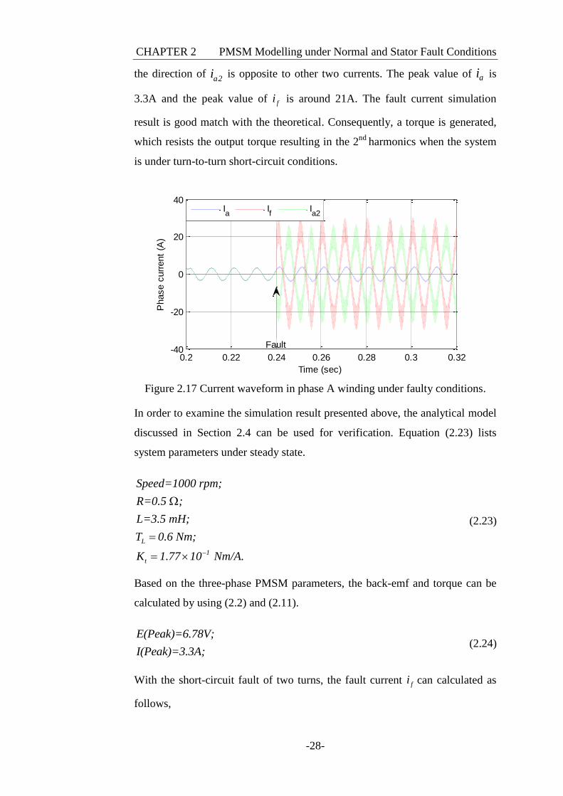
Figure 2.17 Current waveform in phase A winding under faulty conditions. .. 28
Figure 2.18 Torque response under healthy condition (with step change in load).
.......................................................................................................................... 29
Figure 2.19 Speed response under healthy conditions...................................... 30
Figure 2.20 Current response under healthy conditions. .................................. 30
Figure 2.21 Current waveform in phase A winding under healthy conditions. 31
Figure 2.22 Torque response under normal and fault conditions. .................... 31
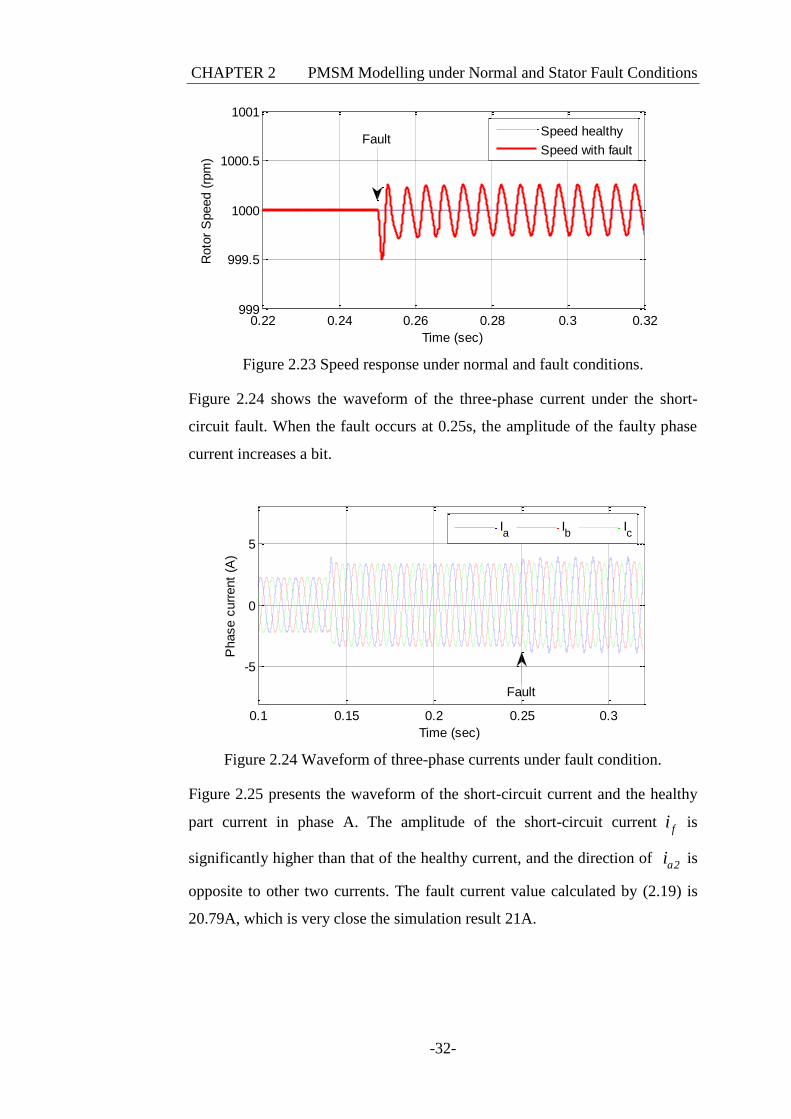
Figure 2.23 Speed response under normal and fault conditions. ...................... 32
Figure 2.24 Waveform of three-phase currents under fault condition.............. 32
Figure 2.25 Current waveform in phase A winding under faulty conditions. .. 33
Figure 3.1 Symmetrical components of unbalanced three-phase system. ........ 37
Figure 3.2 Block diagram of three-phase sequence analyser for negative
sequence components calculation. .................................................................... 39
Figure 3.3 Three-phase current response under balanced system. ................... 40
Figure 3.4 Symmetrical components response under balanced system. ........... 40
Figure 3.5 Three-phase current response under unbalanced system. ............... 41
Figure 3.6 Symmetrical components response under unbalanced system. ....... 42
List of Figures
-IX-
Figure 3.7 Block diagram of the proposed negative sequence calculation
system. .............................................................................................................. 43
Figure 3.8 General structure of SOGI............................................................... 44
Figure 3.9 Bode plots of the SOGI system. ...................................................... 45
Figure 3.10 Three-phase current response under balanced system. ................. 46
Figure 3.11 Comparison of positive sequence components. ............................ 47
Figure 3.12 PMSM speed response under speed fluctuation test. .................... 48
Figure 3.13 Negative sequence current under speed fluctuation and fault
conditions. ......................................................................................................... 49
Figure 3.14 Negative sequence impedance under speed fluctuation and fault
conditions. ......................................................................................................... 49
Figure 3.15 Negative sequence current with moving average filter under speed
fluctuation and fault condition. ......................................................................... 50
Figure 3.16 Block diagram of moving average filter. ...................................... 50
Figure 3.17 Negative sequence impedance with moving average filter under
speed fluctuation and fault condition. ............................................................... 51
Figure 3.18 PMSM torque response under torque fluctuation test. .................. 52
Figure 3.19 Negative-sequence current under load fluctuation and fault
conditions. ......................................................................................................... 52
Figure 3.20 Negative sequence impedance under load fluctuation and fault
conditions. ......................................................................................................... 53
Figure 3.21 Negative sequence current with moving average filter under load
fluctuation and fault condition. ......................................................................... 53
Figure 3.22 Negative sequence impedance with moving average filter under
load fluctuations and fault condition. ............................................................... 54
List of Figures
-X-
Figure 4.1 Example of classical set theory. ...................................................... 57
Figure 4.2 Set V and W in the universe set U. ................................................. 58
Figure 4.3 Union of set V and set W in the universe set U. ............................. 59
Figure 4.4 Intersection of set V and set W in the universe set U. .................... 59
Figure 4.5 Difference of set V and set W in the universe set U. ...................... 60
Figure 4.6 Complement of set V in the universe set U. .................................... 60
Figure 4.7 Fuzzy set of negative sequence impedance. .................................... 61
Figure 4.8 The Mamdani fuzzy inference system. ........................................... 64
Figure 4.9 Centroid of Gravity (COG) method [69]......................................... 65
Figure 4.10 Membership functions for the first input (Negative Sequence
Current). ............................................................................................................ 66
Figure 4.11 Membership functions for the second input “Negative Sequence
Impedance”. ...................................................................................................... 67
Figure 4.12 Membership function for the output “Health and Fault Indicator”.
.......................................................................................................................... 68
Figure 4.13 Fuzzy inference diagram for a healthy PMSM. ............................ 69
Figure 4.14 Fuzzy inference diagram for a faulted PMSM. ............................. 70
Figure 4.15 Fuzzy inference diagram for a PMSM under speed and load
fluctuations. ...................................................................................................... 70
Figure 4.16 Surface plot of the detector response. ........................................... 71
Figure 4.17 PMSM speed response with fault condition. ................................. 72
Figure 4.18 Filtered negative sequence current under speed disturbance. ....... 73
Figure 4.19 Filtered negative sequence impedance under speed disturbance. . 73
List of Figures
-XI-
Figure 4.20 Fault indicator under speed disturbance and fault condition......... 74
Figure 4.21 PMSM torque response under fault condition............................... 74
Figure 4.22 Filtered negative sequence current under load disturbance and 2
turns fault. ......................................................................................................... 75
Figure 4.23 Filtered negative sequence impedance under load disturbance and
2 turns fault. ...................................................................................................... 75
Figure 4.24 Fault indicator under load disturbance and 2 turns fault. .............. 76
Figure 4.25 Torque response under fault condition. ......................................... 76
Figure 4.26 Filtered negative sequence current under load disturbance 10 turns
fault. .................................................................................................................. 77
Figure 4.27 Filtered negative sequence impedance under load disturbance and
10 turns fault. .................................................................................................... 77
Figure 4.28 Fault indicator under load disturbance and 10 turns fault. ............ 78
Figure A.1 Simulink model of vector controlled PMSM. ................................ 82
Figure A.2 Subsystem of the PMSM. ............................................................... 83
Figure A.3 Subsystem of the electrical model. ................................................. 83
Figure A.4 Subsystem of back-emf model. ...................................................... 84
Figure A.5 Simulink model of FDD. ................................................................ 84
Figure A.6 Subsystem of negative sequence components model. .................... 85
List of Tables
-XII-
List of Tables
Table 2.1 Three-phase PMSM parameters ....................................................... 19
Table 3.1 Relationship between the sequence components under load change,
speed change and fault condition. ..................................................................... 55
Table 4.1 Notations and definitions of the set example shown in Figure 4.1... 58
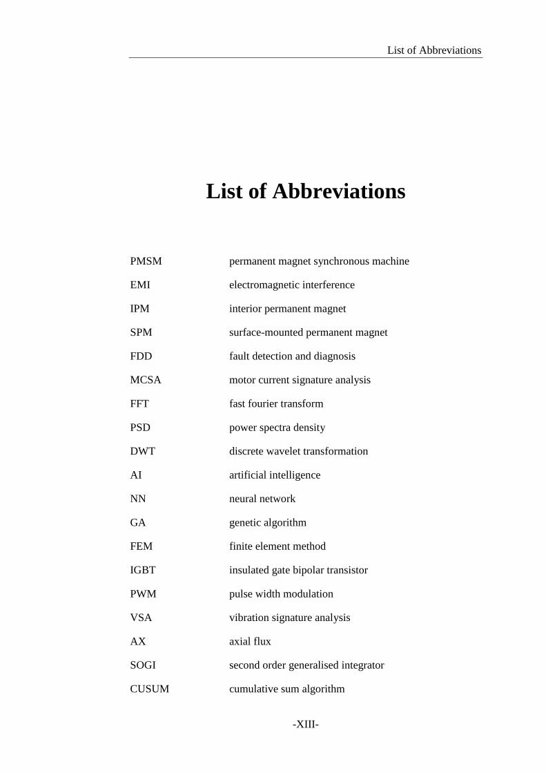
List of Abbreviations
-XIII-
List of Abbreviations
PMSM permanent magnet synchronous machine
EMI electromagnetic interference
IPM interior permanent magnet
SPM surface-mounted permanent magnet
FDD fault detection and diagnosis
MCSA motor current signature analysis
FFT fast fourier transform
PSD power spectra density
DWT discrete wavelet transformation
AI artificial intelligence
NN neural network
GA genetic algorithm
FEM finite element method
IGBT insulated gate bipolar transistor
PWM pulse width modulation
VSA vibration signature analysis
AX axial flux
SOGI second order generalised integrator
CUSUM cumulative sum algorithm

List of Abbreviations
-XIV-
CCVSI current-controlled voltage source inverter
PLL phase locked loop
CHAPTER 1 Introduction
-1-
CHAPTER 1
INTRODUCTION
1.1 Electrical Machines
Built on the foundation of electromagnetic phenomena, electrical machines
were first invented early in the 19th
century. By the classic definition, electrical
machine is the universal name of both electrical motors and generators, which
are both electromechanical energy converters (i.e. converting energy between
electrical and mechanical forms). Nowadays, most of the electricity consumed
by humans is generated by electrical generators, and more than 60% of the
electricity is consumed by different types of electrical motors. Hence, the
electrical machine is ubiquitous and important in modern social and industrial
applications.
There are many different ways to classify electrical machines (motors or
generators), such as electrical power input (DC or AC), operating condition
(AC induction or AC synchronous), and rotor structure (switching reluctance
machines) etc. Permanent magnet synchronous machines (PMSMs) were not
widespread until the middle of last century. Especially in the 1980s, industrial
CHAPTER 1 Introduction
-2-
manufacturers made progress in the improvement of the magnet characteristics,
which enabled the fast development of the PMSMs [1, 2]. Compared to the
traditional induction motors, the PMSMs utilise a permanent magnet to create
magnetic field instead of using winding coils. This important feature brings the
PMSMs with many advantages, such as higher power density, lower
electromagnetic interference (EMI), higher achievable motor speed etc.
Therefore, the PMSMs have been extensively used in modern industrial
applications, such as hybrid automobile, aerospace drives.
1.2 Permanent Magnet Synchronous Machines
For PMSMs, the stator generally has the same form as traditional induction
motors, i.e. classical three-phase stator windings. Instead of excitation
windings, the rotor of the PMSM’s rotor has the permanent magnet installed
which is responsible for the creation of the magnetic field. According to the
position of the magnet, the PMSM can be roughly divided into two categories,
which are the interior permanent magnet (IPM) motor type and the surface
mounted permanent magnet (SPM) motor type [3].
For the SPM motors, the permanent magnet is installed directly on the surface
of the cylindrical rotor, which implies that the magnetic flux path seen by the
stator windings is independent of rotor position. In contrast, the permanent
magnet of the IPM motors is buried inside the rotor, which leads to magnetic
reluctance variation with rotor position. Consequently, the synchronous
inductance, Ld, in the direction of the rotor magnetic axis is the same as Lq, the
inductance in the quadrature direction in SPM machine, but is different in
IPMs.
Each type PMSM has its own advantages and drawbacks. In general, the SPM
motor is relatively easy to construct and has low torque ripple and good
linearity; due to the buried magnet structure, the IPM motor is difficult to build
and thus the cost is slightly higher. However, the constant power capability of
the IPM is better than the SPM motors [3].
CHAPTER 1 Introduction
-3-
Although the use of the permanent magnet brings many merits, the PMSM is
very sensitive to machine or control system faults, since the magnetic field
generated by the PM cannot be turned off at will. For instance, a few short-
circuit turns of the stator winding will lead to an increment in the faulted
winding current, and thus to excessive heat generation. This may further
propagate and eventually cause a catastrophic failure.
If the control and protection system can detect abnormal events at early stage,
the catastrophic failures can be avoided and the machine can be protected.
Particularly for applications demanding high security and reliability (e.g.
aerospace and automotive sectors), fault detection of the PMSMs has become
crucially important and attracted much interest.
1.3 Fault Detection and Diagnosis
1.3.1 Introduction
Fault detection and diagnosis (FDD) plays a very important role for the PMSM
operation in many industrial applications. In the real word, the engineering
system is inherently complex, and faults are difficult to avoid. A simple fault
may result in the whole engineering system shut-down, and potential
equipment damage, etc. Due to the above reasons, FDD is of great practical
significance.
Figure 1.1 illustrates the block diagram of a general FDD system. The
electrical machine system is regulated by a controller and using feedback
signals from the measurement sensors. A FDD system is applied to monitor
both the control output and sensor measurements, in order to analyse the data
and thus judge the machine operating condition. As long as any abnormal
signal is observed, the FDD sends high priority control commands to protect
the machine from possible faults. It should be pointed out that, the machine
system and measurement device are subject to faults, disturbance and
environmental noise; the disturbances and sensor noise can result in a
misjudgement of the machine operating condition. It is, therefore, essential that
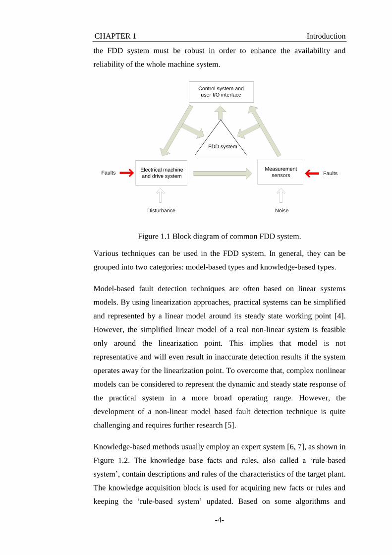
CHAPTER 1 Introduction
-4-
the FDD system must be robust in order to enhance the availability and
reliability of the whole machine system.
Electrical machine
and drive system
Measurement
sensors
Control system and
user I/O interface
FDD system
Disturbance Noise
FaultsFaults
Figure 1.1 Block diagram of common FDD system.
Various techniques can be used in the FDD system. In general, they can be
grouped into two categories: model-based types and knowledge-based types.
Model-based fault detection techniques are often based on linear systems
models. By using linearization approaches, practical systems can be simplified
and represented by a linear model around its steady state working point [4].
However, the simplified linear model of a real non-linear system is feasible
only around the linearization point. This implies that model is not
representative and will even result in inaccurate detection results if the system
operates away for the linearization point. To overcome that, complex nonlinear
models can be considered to represent the dynamic and steady state response of
the practical system in a more broad operating range. However, the
development of a non-linear model based fault detection technique is quite
challenging and requires further research [5].
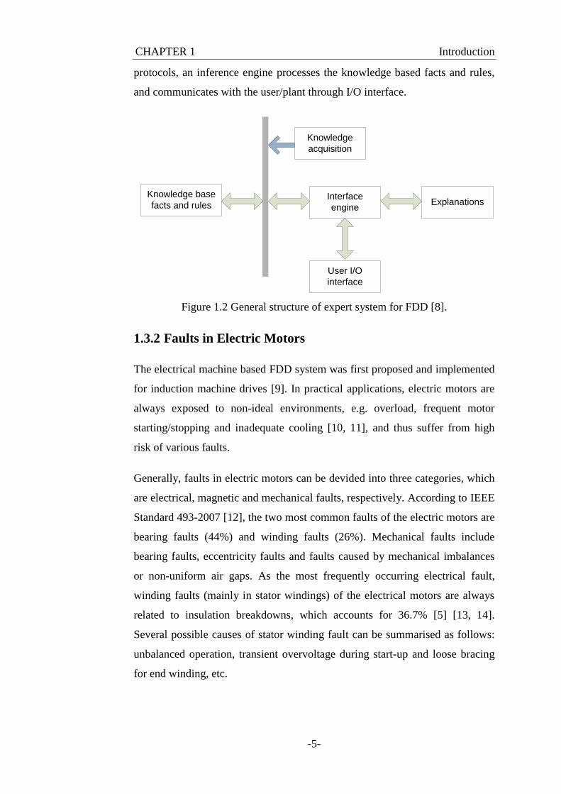
Knowledge-based methods usually employ an expert system [6, 7], as shown in
Figure 1.2. The knowledge base facts and rules, also called a ‘rule-based
system’, contain descriptions and rules of the characteristics of the target plant.
The knowledge acquisition block is used for acquiring new facts or rules and
keeping the ‘rule-based system’ updated. Based on some algorithms and
CHAPTER 1 Introduction
-5-
protocols, an inference engine processes the knowledge based facts and rules,
and communicates with the user/plant through I/O interface.
Knowledge base
facts and rules
Knowledge
acquisition
Interface
engine
User I/O
interface
Explanations
Figure 1.2 General structure of expert system for FDD [8].
1.3.2 Faults in Electric Motors
The electrical machine based FDD system was first proposed and implemented
for induction machine drives [9]. In practical applications, electric motors are
always exposed to non-ideal environments, e.g. overload, frequent motor
starting/stopping and inadequate cooling [10, 11], and thus suffer from high
risk of various faults.
Generally, faults in electric motors can be devided into three categories, which
are electrical, magnetic and mechanical faults, respectively. According to IEEE
Standard 493-2007 [12], the two most common faults of the electric motors are
bearing faults (44%) and winding faults (26%). Mechanical faults include
bearing faults, eccentricity faults and faults caused by mechanical imbalances
or non-uniform air gaps. As the most frequently occurring electrical fault,
winding faults (mainly in stator windings) of the electrical motors are always
related to insulation breakdowns, which accounts for 36.7% [5] [13, 14].
Several possible causes of stator winding fault can be summarised as follows:
unbalanced operation, transient overvoltage during start-up and loose bracing
for end winding, etc.
CHAPTER 1 Introduction
-6-
Starting with an insignificant insulation failure between winding turns, this
kind of fault may not have much noticeable effect at initial. However, it can
quickly develop into phase loss and propagates quickly to other serious faults,
and even lead to a catastrophic failure of the entire machine system [15, 16].
1.3.3 FDD Techniques in Electrical Motors
In the literature, various FDD techniques have been presented and
demonstrated for electrical machine systems, and each fault detection
technique has its own merits and limitations. Several classical approaches are
studied and reviewed as follows.
Motor current signature analysis (MCSA) is a common solution that had been
used for both induction motors and PMSMs [17]. In [18], the fast Fourier
Transform (FFT) of the rotor current was monitored to diagnose faults of
induction machines. However, this method does not perform well when the
machine is subject to fluctuations (e.g. speed or load changes). This is because
these fluctuations imply variations on the motor slips and thus the FFT signals.
Therefore, this approach is not always reliable and the fault detection result
should be treated cautiously to avoid false alarms.
With the aim of overcoming this limitation, a method based on the sequence
components of the machine current variables was developed in [19] for fault
diagnosis of induction machines. The inherent asymmetries of the system were
removed by using pre-recorded information of sequence components under
system normal conditions to isolate the fault signal and improve the reliability
of the detection result.
The wavelet transform is also a suitable approach to assess motor faults under
limited speed and load variation. For example in [20], the wavelet analysis of
the winding current is combined with power spectral density (PSD) estimation,
in order to detect inter-turn short-circuit faults of inductor motors. The wavelet
analysis based PMSM fault detection approach was discussed in [21]. The
stator current harmonics have noticeable relevance with inter-turn short-circuit
of the PMSM, compared with normal conditions.
CHAPTER 1 Introduction
-7-
The discrete wavelet transformation (DWT) has been used in [22-25], as an
alternative tool for fault feature extraction to detect different electrical faults
under non-stationary conditions, inter-turn fault, bearing damage, etc. Barendse
et al [22] have applied the DWT to analyse the current variables on the rotating
frame. Bearing damage of the PMSMs was detected by using DWT over a
wide speed range [23].
Recently, sequence component theory has been considered by many
researchers as an promising solution for an electrical machine FDD system.
Cheng et al. have demonstrated that using the sequence component approach
can detect stator winding faults in induction motors [26]. The value of
negative-positive-sequence impedance is dependent on the asymmetric
behaviour of the machine, which is sensitive to stator short-circuit fault (even if
there is a one-turn stator fault). However, the main limitation of this method is
that. It demands independent current measurement [26]. In [27], the zero
sequence component of the stator voltage variables was proposed for assessing
winding faults when the motor speed changes. However, in the above
mentioned papers, the developed methodologies have only considered the
diagnosis procedure under load fluctuations, i.e. the influence of speed change,
or frequency change, is not addressed.
In the last decade, artificial Intelligence (AI) techniques have attracted much
interest and have been employed successfully in the fault detection area. The
solicitation of expert systems, fuzzy logic theory, genetic algorithm (GA) and
artificial intelligent neural networks (NN) has been considered for fault
diagnosis of electric motor drive systems [28, 29]. A fuzzy logic based MCSA
approach was discussed in [28], to detect inter-turn short-circuit faults in
induction motors. In [30], the authors focused on the open-loop systems and
applied a feed-forward NN to detect inter-turn faults. However, for all the AI
techniques, a new set of training data is required when applying the technique
to a new machine.
CHAPTER 1 Introduction
-8-
1.4 Project Objectives
Based on the above discussion an effective and reliable FDD scheme is vital
for PMSM applications that demand high reliability and high security. The
objective of this research work is to develop a novel fault detection and
diagnosis system, which is capable of assessing, quickly and reliably, inter-turn
short-circuit faults in PMSMs. The developed fault detection scheme integrates
the negative sequence component analysis with fuzzy logic classifier, to
improve sensitivity and robustness detection.
The main topics covered in the thesis are:
Development of a parametric model to simulate the operation of a
PMSM drive under both normal and fault conditions.
Development of a detection technique to diagnose inter-turn short-
circuit faults in PMSMs, based on negative sequence component
analysis of stator current and voltage signals.
Application of fuzzy logic classifier to improve the robustness of the
sequence component analysis techniques and thereby enhance the
reliability of the FDD system.
1.5 .Thesis Outline
The thesis is sectioned into five chapters as follows:
Chapter 2 develops a simulation model of a three-phase PMSM drive system
with inter-turn short-circuit faults and performs simulation study of fault
behaviour.
Chapter 3 presents a detailed literature review of fault detection techniques for
both induction motors and PMSMs. The concept of symmetrical components is
introduced and reviewed. Following this, two methods for the real-time
evaluation of sequence components of the PMSM are compared and discussed.
The utility of the sequence component analysis for detecting inter-turn faults is
CHAPTER 1 Introduction
-9-
studied, and the influences of load and speed fluctuations on the negative
sequence components are highlighted and analysed.
Chapter 4 applies the fuzzy logic approach for the FDD of an inter-turn short-
circuit fault in PMSM drives under load or speed change. The fundamental
theory of classical set and fuzzy set is introduced as the basis of the fuzzy logic
theory. Then, the membership function and the rule based inference of the
fuzzy logic are discussed to provide a clear understanding of the concepts.
Finally, the simulation shows that the proposed approach is capable of
diagnosing faults accurately and quickly under both load and speed fluctuations.
Chapter 5 summarises the contribution of this research and discusses possible
future work.
CHAPTER 2 PMSM Modelling under Normal and Stator Fault Conditions
-10-
CHAPTER 2
PMSM MODELLING UNDER
NORMAL AND STATOR
FAULT CONDITIONS
2.1 Introduction
In the last two decades, permanent magnet synchronous machines (PMSM)
have been widely investigated and applied in modern industrial areas, such as
hybrid vehicles, electric trains, airplanes and military power drive applications
[13, 21], due to their higher torque, higher efficiency and better dynamic
performance in comparison to traditional machines with electromagnetic
excitation. However, the presence of the spinning rotor magnets is a significant
weak point for the PMSMs, and any fault may create special challenges. With
the aim of ensuring high system reliability and extending motor life, fault
detection of the PMSMs plays an important role and attracts more and more
interest.
Generally, there are three kinds of faults in the PMSMs: electrical faults,
magnetic faults and mechanical faults. Since magnetic faults and mechanical
CHAPTER 2 PMSM Modelling under Normal and Stator Fault Conditions
-11-
faults are not related to this research work, only electrical faults will be
considered. An electrical fault is typically caused by the failure of winding
insulation, and can be further divided into three categories which are turn to
turn, phase to phase and phase to ground faults. As the most common fault in
the electrical machines, the turn-to-turn fault is particularly difficult to detect.
This is because, when an inter-turn short-circuit fault takes place, the current
under feedback control may not have much noticeable change. However, the
current in the short-circuit turns can be many times greater than the permissible
level [31]. In contrast, if a terminal short-circuit occurs, the current is limited
by the phase inductance. This feature implies the machine would withstand a
phase terminal short-circuit indefinitely if the phase inductance is per unit and
continued operation on the healthy phases. Since the fault current has a phase
shift of 90 degrees with the back-emf, neglecting fault resistance, the resultant
average torque output is small [32]. Nevertheless, the induced heat may lead to
phase to phase and phase to ground faults.
Therefore, the effective modelling of the PMSM inter-turn short-circuit faults
is becoming crucially important in the development of fault diagnosis. It would
appear that a model with high precision would be the better for this purpose.
However, in reality, a compromise needs to be made between the accuracy and
the complexity of the model. A promising model of the PMSM inter-turn fault
should be able to describe the behaviour of one turn fault functionally and to
account for the effects of the fault correctly [33].
A finite element method (FEM) approach was presented in [34, 35] to analyse
the stator winding faults and inter-turns short-circuit faults. Obviously, the
FEM modelling does give quite accurate results since it includes most of the
physical phenomena. However, it demands a detailed machine specification
and a long computational time. For this reason, the FEM models are often
applied only in the fault study cases rather than in detection schemes [36]. To
overcome the limitations of the FEM model, a classical dynamic model based
on the three-phase circuit coordinates has been used in this work.
CHAPTER 2 PMSM Modelling under Normal and Stator Fault Conditions
-12-
2.2 PMSM Healthy Condition
In this section, the transformation of the PMSM equation from the three-phase
axis (ABC) to the rotating frame (DQ) is presented.
2.2.1 Brushless AC Motors in Stator ABC system
Considering a star-connected three-phase brushless AC motor with high
resistivity magnet and retaining sleeves, the current components induced by the
rotor can be ignored [37]. Therefore, the circuit equations of the three
perfectly-balanced windings, i.e. no physical discrepancy between the
windings, can be described in (2.1),
a
b
c
a a a ac a aab
b b ab b bc b b
c c ac c c cbc
v R 0 0 i L M M i ed
v 0 R 0 i M L M i edt
v 0 0 R i M M L i e
(2.1)
where av , bv and cv represent the three-phase voltages; ai , bi and ci are the
phase currents of the three windings; aR , bR and cR are the resistance of the
windings; aL , bL and cL represent the self-inductance of each phase, while abM ,
acM and bcM are the mutual inductance between them; ae , be and ce represent
the back-emf of each phase.
Equation (2.2) presents two sources of the back-emf T
a b ce e e , i.e. one
from the flux linkage m and another from the electrical angular speed .
mm
a
m mb
c
m m
2π
3
2π 2π π
3 3 2
2π 2π π
3 3 2
(cos t )sin t
e
e = (sin t ) (cos t )
e(sin t ) (cos t + )
(2.2)
The electrical angular speed is determined by the pole pairs P times and the
mechanical angular speed m , as given in (2.3).
CHAPTER 2 PMSM Modelling under Normal and Stator Fault Conditions
-13-
mP (2.3)
Assuming that the rotor reluctance stays constant, the self-inductance and
mutual inductance of the three windings can be considered identical to each
other [38], which yields,
a cb
a cb
acab bc
R R R R
L L L L
M M M M
(2.4)
The sum of the three-phase currents for a star-connected balanced machine
equals out zero.
a cbi i i 0 (2.5)
Based on the above definitions, (2.1) can be re-written as in (2.6).
a a a a
b b b b
c c c c
v R 0 0 i L M M i ed
v 0 R 0 i M L M i edt
v 0 0 R i M M L i e
(2.6)
The electromagnetic torque eT can be derived as in (2.7), where LT , J and B
represent the load torque, moment of inertia and viscous friction coefficient of
the motor, respectively.
a a c cb be
m
mmL
e i e i e iT
d =T B J
dt
(2.7)
Therefore, the mechanical angular speed can be obtained as in (2.8).
e mLm
T T B( )dt
J
(2.8)
CHAPTER 2 PMSM Modelling under Normal and Stator Fault Conditions
-14-
2.2.2 Park’s Transformation
The Park’s Transformation (also known as DQ transformation) has been first
proposed by Robert H. Park [39] in 1929. As a mathematical transformation, it
rotates the reference frame of three-phase systems in an effort to simplify the
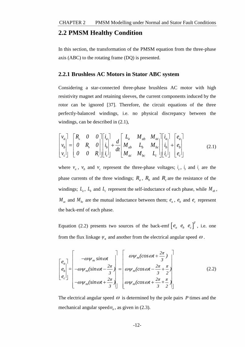
analysis of three-phase circuits. Figure 2.1 presents the physical interpretation
of this transformation, where θ defines the angle between the d-axis and a
stationary reference frame – usually the a-axis for simplicity.
a
c
b
dq
θ
Figure 2.1 DQ rotating reference frame.
The Park’s transformation can be represented by (2.9), where the variable x can
be current, voltage or back-emf.
ad
dq abc bq
c
dq abc
2π 2π
3 3
2π 2π
3 3
xx
C x ;x
x
cos cos( - ) cos( )2
C3
-sin - sin( - ) - sin( )
(2.9)
Combining it with (2.6), the three-phase PMSM model can be rewritten as in
(2.10), where e mK =P is the back-emf constant, and d qL L L-M .
CHAPTER 2 PMSM Modelling under Normal and Stator Fault Conditions
-15-
qd d dd
q q qq e md
v i i- L L 0R 0d
dtv i i0 L KL R
(2.10)
The torque equation in the DQ frame can be derived as in (2.11), where
t m
3
2K = P is the torque constant.
e q qd dm
m q q qd d
m q
t q
3T ( v i v i )
2
3P = i ( L -L )i i
23P
= i2
=K i
(2.11)
2.3 PMSM under Fault Condition
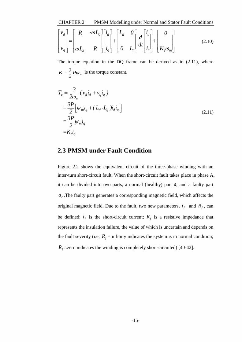
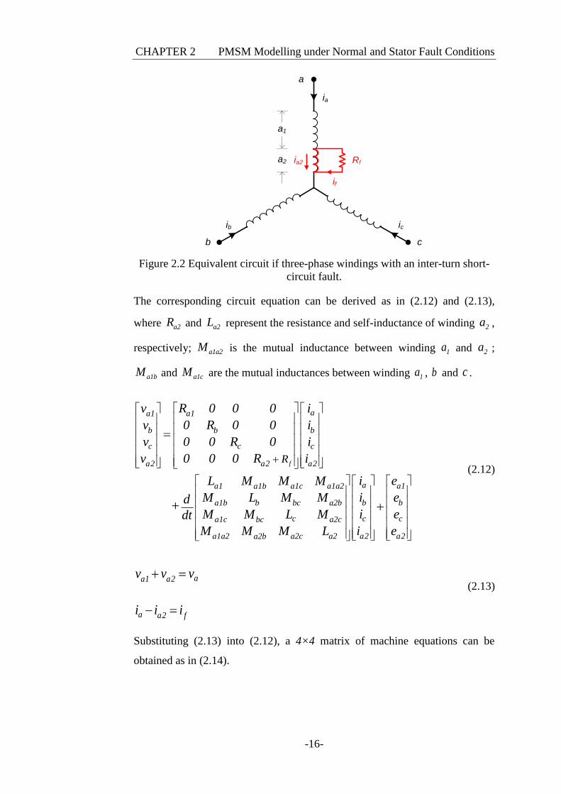
Figure 2.2 shows the equivalent circuit of the three-phase winding with an
inter-turn short-circuit fault. When the short-circuit fault takes place in phase A,
it can be divided into two parts, a normal (healthy) part 1a and a faulty part
2a .The faulty part generates a corresponding magnetic field, which affects the
original magnetic field. Due to the fault, two new parameters, fi and fR , can
be defined: fi is the short-circuit current; fR is a resistive impedance that
represents the insulation failure, the value of which is uncertain and depends on
the fault severity (i.e. fR = infinity indicates the system is in normal condition;
fR ≈zero indicates the winding is completely short-circuited) [40-42].
CHAPTER 2 PMSM Modelling under Normal and Stator Fault Conditions
-16-
a
b
ia
ib ic
c
a1
a2 Rf
if
ia2
Figure 2.2 Equivalent circuit if three-phase windings with an inter-turn short-
circuit fault.
The corresponding circuit equation can be derived as in (2.12) and (2.13),
where a2R and a2L represent the resistance and self-inductance of winding 2a ,
respectively; a1a2M is the mutual inductance between winding 1a and 2a ;
a1bM and a1cM are the mutual inductances between winding 1a , b and c .
f
aa1a1
bb b
cc c
a2a2 a2
a a1a1 a1c a1a2a1b
ba1b b bc a2b
cca1c a2cbc
a2a1a2 a2c a2a2b
R
R 0 0 0v i
0 R 0 0v i
0 0 R 0v i
0 0 0 Rv i
i eL M M M
iM L M Md
iM M L Mdt
iM M M L
+
b
c
a2
e
e
e
(2.12)
aa1 a2
a a2 f
v v v
i i i
(2.13)
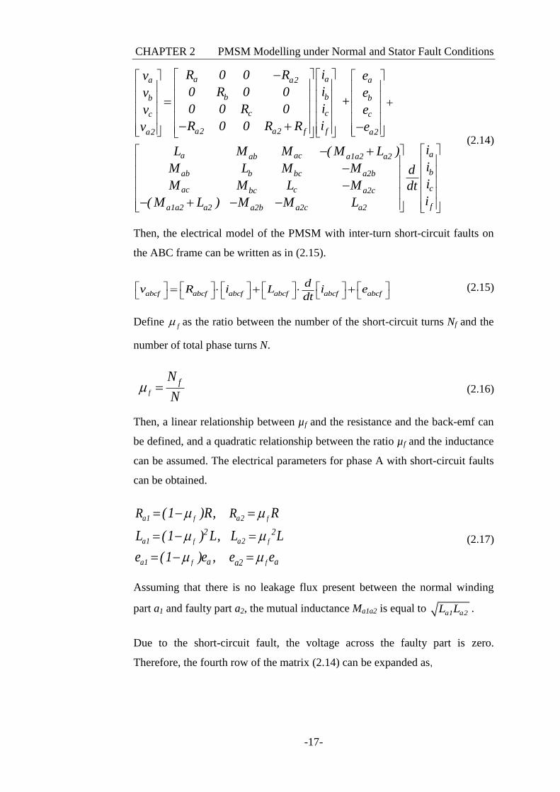
Substituting (2.13) into (2.12), a 4×4 matrix of machine equations can be
obtained as in (2.14).
CHAPTER 2 PMSM Modelling under Normal and Stator Fault Conditions
-17-
aaa aa2
bbb b
ccc c
fa2 a2 fa2 a2
a ac a1a2 a2ab
ab b bc a2b
ac c a2cbc
a1a2 a2 a2c a2a2b
iR 0 0 Rv e
i0 R 0 0v e +
i0 0 R 0v e
iR 0 0 R Rv e
L M M ( M L )
M L M M
M M L M
( M L ) M M L
a
b
c
f
i
ididt
i
(2.14)
Then, the electrical model of the PMSM with inter-turn short-circuit faults on
the ABC frame can be written as in (2.15).
abcf abcf abcf abcf abcf abcf
dv R i L i e
dt
(2.15)
Define f as the ratio between the number of the short-circuit turns Nf and the
number of total phase turns N.
f
fN
N (2.16)
Then, a linear relationship between µf and the resistance and the back-emf can
be defined, and a quadratic relationship between the ratio µf and the inductance
can be assumed. The electrical parameters for phase A with short-circuit faults
can be obtained.
f f
f f
f f
a1 a2
a1 a2
a1
2 2
a aa2
R R(1 )R, R
L (1 ) L, L L
e (1 )e , e e
(2.17)
Assuming that there is no leakage flux present between the normal winding
part a1 and faulty part a2, the mutual inductance Ma1a2 is equal to a1 a2L L .
Due to the short-circuit fault, the voltage across the faulty part is zero.
Therefore, the fourth row of the matrix (2.14) can be expanded as,
CHAPTER 2 PMSM Modelling under Normal and Stator Fault Conditions
-18-
a2
f
a2 a2 f
a b caa2 a2 a1a2 a2c a2a2b
v 0
diL R i
dt
didi diR i ( L M ) M M e
dt dt dt
(2.18)
Assuming the resistive impedance Rf that models the insulation failure is zero,
based on the definitions in (2.17), the short-circuit current if in steady state can
be derived as in (2.19).
f
a b ca.rated a a a ab ac a
a.rated
fa a2
di di div R i L M M e
dt dt dt
vi
R j L
(2.19)
The electromagnetic torque (2.7) can be re-written as follows, where
c ca1 a1 a2 a2b be
m
a a c c a2b b f
m
e i e i e i e iT
e i e i e i e i
(2.20)
2.4 Modelling PMSM under Inter-Turn Fault
The previous section has presented the mathematical equation of the PMSM
with inter-turn short-circuit faults. In this section, a simulation model is
established by using the Matlab/Simulink platform, according to the PMSM
machine specification.
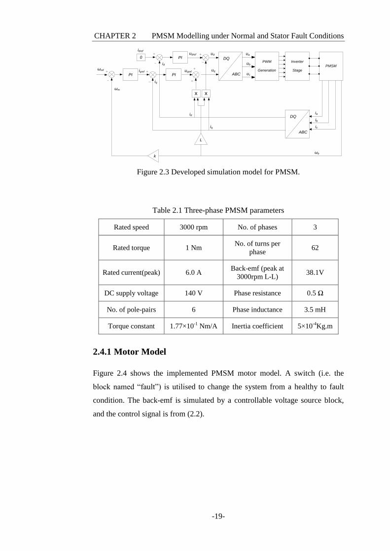
Figure 2.3 shows the developed simulation model, while Table 2.1 summarises
the nominal parameters of the PMSM. The model consists of the control block,
the PMSM motor block (electrical model, mechanical model and back-emf
model), the inverter stage and the d-q reference frame transformation block,
which will be discussed in detail as follows.
CHAPTER 2 PMSM Modelling under Normal and Stator Fault Conditions
-19-
ωref
ωm
PIiqref
iq
PIuqref uq
PIudref
id
0
idrefud ua
ub
uc
ia
ib
ic
DQ
ABC
PWM
Generation
Inverter
Stage
PMSM
DQ
ABC
x x
ωek
L
id
iq
Figure 2.3 Developed simulation model for PMSM.
Table 2.1 Three-phase PMSM parameters
Rated speed 3000 rpm No. of phases 3
Rated torque 1 Nm No. of turns per
phase 62
Rated current(peak) 6.0 A Back-emf (peak at
3000rpm L-L) 38.1V
DC supply voltage 140 V Phase resistance 0.5 Ω
No. of pole-pairs 6 Phase inductance 3.5 mH
Torque constant 1.77×10⁻¹
Nm/A Inertia coefficient 5×10⁻⁴
Kg.m
2.4.1 Motor Model
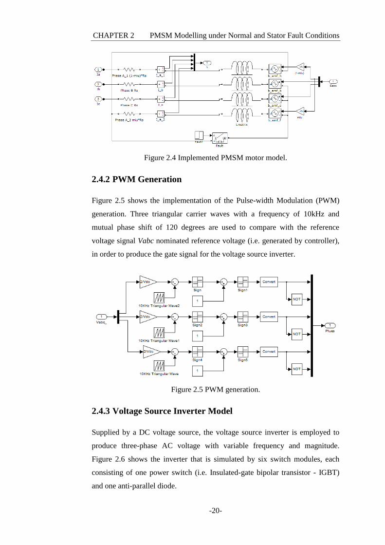
Figure 2.4 shows the implemented PMSM motor model. A switch (i.e. the
block named “fault”) is utilised to change the system from a healthy to fault
condition. The back-emf is simulated by a controllable voltage source block,
and the control signal is from (2.2).
CHAPTER 2 PMSM Modelling under Normal and Stator Fault Conditions
-20-
Figure 2.4 Implemented PMSM motor model.
2.4.2 PWM Generation
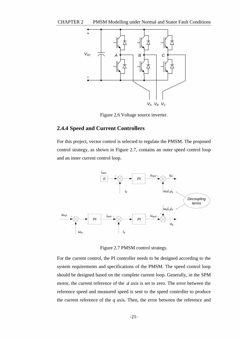
Figure 2.5 shows the implementation of the Pulse-width Modulation (PWM)
generation. Three triangular carrier waves with a frequency of 10kHz and
mutual phase shift of 120 degrees are used to compare with the reference
voltage signal Vabc nominated reference voltage (i.e. generated by controller),
in order to produce the gate signal for the voltage source inverter.
Figure 2.5 PWM generation.
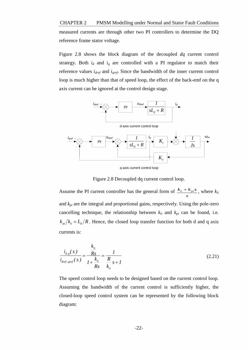
2.4.3 Voltage Source Inverter Model
Supplied by a DC voltage source, the voltage source inverter is employed to
produce three-phase AC voltage with variable frequency and magnitude.
Figure 2.6 shows the inverter that is simulated by six switch modules, each
consisting of one power switch (i.e. Insulated-gate bipolar transistor - IGBT)
and one anti-parallel diode.
CHAPTER 2 PMSM Modelling under Normal and Stator Fault Conditions
-21-
VDC A B C
VA VB VC
Figure 2.6 Voltage source inverter.
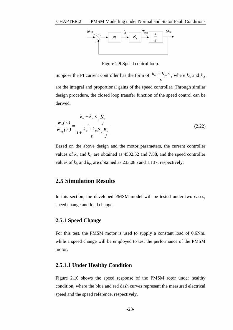
2.4.4 Speed and Current Controllers
For this project, vector control is selected to regulate the PMSM. The proposed
control strategy, as shown in Figure 2.7, contains an outer speed control loop
and an inner current control loop.
ωref
ωm
PIiqref
iq
PIuqref
uq
PIudref
id
0
idrefud
ωeLqiq
ωeLdid
Decoupling
terms
Figure 2.7 PMSM control strategy.
For the current control, the PI controller needs to be designed according to the
system requirements and specifications of the PMSM. The speed control loop
should be designed based on the complete current loop. Generally, in the SPM
motor, the current reference of the d axis is set to zero. The error between the
reference speed and measured speed is sent to the speed controller to produce
the current reference of the q axis. Then, the error between the reference and
CHAPTER 2 PMSM Modelling under Normal and Stator Fault Conditions
-22-
measured currents are through other two PI controllers to determine the DQ
reference frame stator voltage.
Figure 2.8 shows the block diagram of the decoupled dq current control
strategy. Both id and iq are controlled with a PI regulator to match their
reference values idref and iqref. Since the bandwidth of the inner current control
loop is much higher than that of speed loop, the effect of the back-emf on the q
axis current can be ignored at the control design stage.
PIudref
d
1
sL R
PI
uqref
d
1
sL RtK
1
Js
eK
ididref
iqrefiq ωm
d-axis current control loop
q-axis current control loop
Figure 2.8 Decoupled dq current control loop.
Assume the PI current controller has the general form of ii pik k s
s
, where kii
and kpi are the integral and proportional gains, respectively. Using the pole-zero
cancelling technique, the relationship between kii and kpi can be found, i.e.
pi ii dk k L R . Hence, the closed loop transfer function for both d and q axis
currents is:
ii
d ,q
iidref ,qref
ii
ki ( s ) 1Rs
k Ri ( s )s 11
kRs
(2.21)
The speed control loop needs to be designed based on the current control loop.
Assuming the bandwidth of the current control is sufficiently higher, the
closed-loop speed control system can be represented by the following block
diagram:
CHAPTER 2 PMSM Modelling under Normal and Stator Fault Conditions
-23-
PI tK1
J
iq ωmωref Tem
Figure 2.9 Speed control loop.
Suppose the PI current controller has the form of is psk k s
s
, where kis and kps
are the integral and proportional gains of the speed controller. Through similar
design procedure, the closed loop transfer function of the speed control can be
derived.
is ps t
m
is ps tref
k k s K
w ( s ) s Jk k s Kw ( s )
1s J
(2.22)
Based on the above design and the motor parameters, the current controller
values of kii and kpi are obtained as 4502.52 and 7.58, and the speed controller
values of kis and kps are obtained as 233.085 and 1.137, respectively.
2.5 Simulation Results
In this section, the developed PMSM model will be tested under two cases,
speed change and load change.
2.5.1 Speed Change
For this test, the PMSM motor is used to supply a constant load of 0.6Nm,
while a speed change will be employed to test the performance of the PMSM
motor.
2.5.1.1 Under Healthy Condition
Figure 2.10 shows the speed response of the PMSM rotor under healthy
condition, where the blue and red dash curves represent the measured electrical
speed and the speed reference, respectively.
CHAPTER 2 PMSM Modelling under Normal and Stator Fault Conditions
-24-
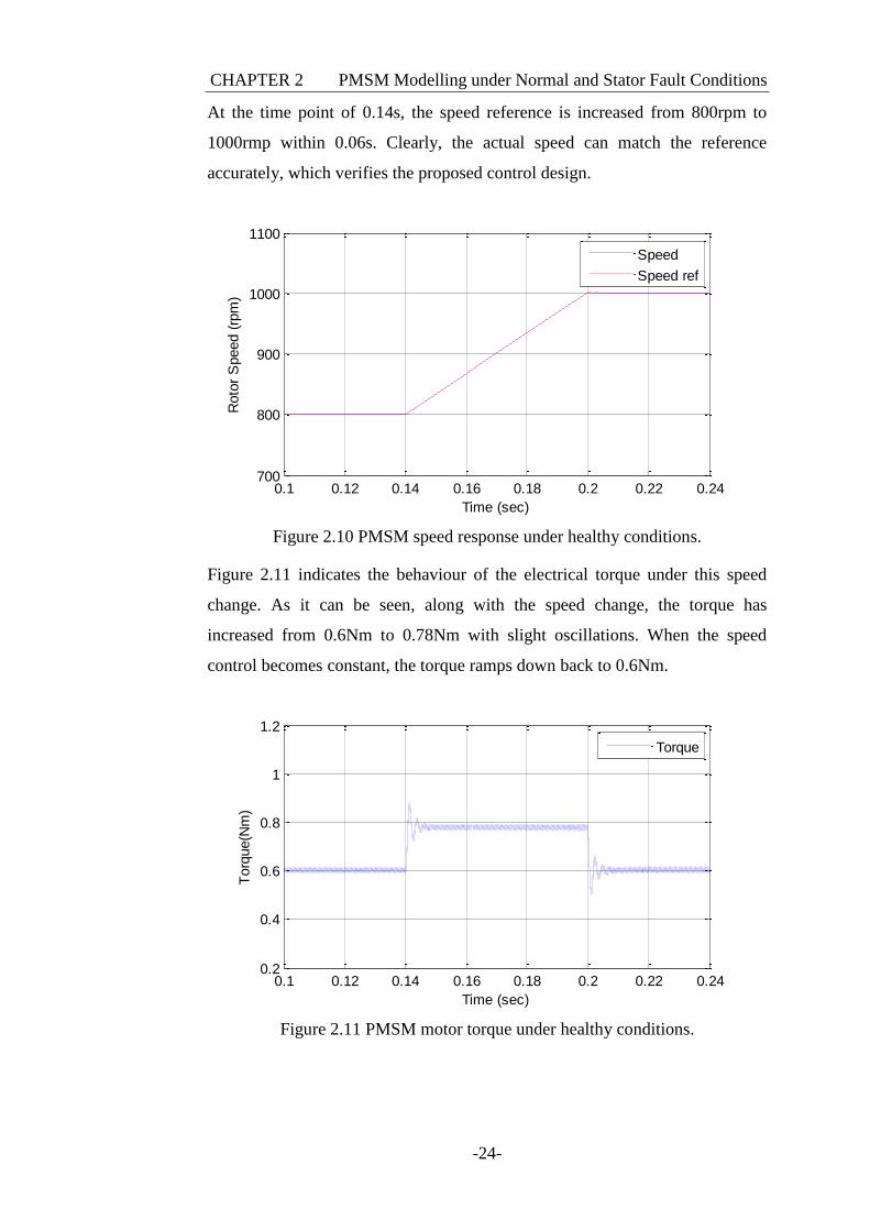
At the time point of 0.14s, the speed reference is increased from 800rpm to
1000rmp within 0.06s. Clearly, the actual speed can match the reference
accurately, which verifies the proposed control design.
Figure 2.10 PMSM speed response under healthy conditions.
Figure 2.11 indicates the behaviour of the electrical torque under this speed
change. As it can be seen, along with the speed change, the torque has
increased from 0.6Nm to 0.78Nm with slight oscillations. When the speed
control becomes constant, the torque ramps down back to 0.6Nm.
Figure 2.11 PMSM motor torque under healthy conditions.
0.1 0.12 0.14 0.16 0.18 0.2 0.22 0.24700
800
900
1000
1100
Time (sec)
Roto
r S
peed (
rpm
)
Speed
Speed ref
0.1 0.12 0.14 0.16 0.18 0.2 0.22 0.240.2
0.4
0.6
0.8
1
1.2
Time (sec)
Torq
ue(N
m)
Torque
CHAPTER 2 PMSM Modelling under Normal and Stator Fault Conditions
-25-
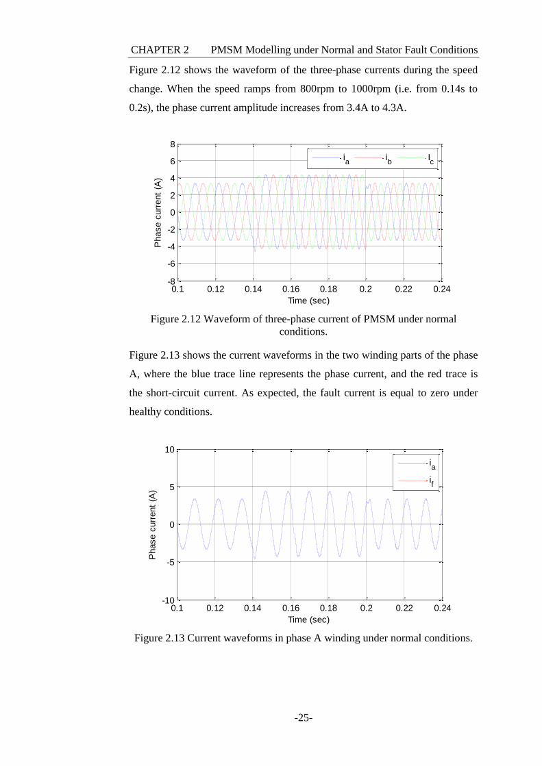
Figure 2.12 shows the waveform of the three-phase currents during the speed
change. When the speed ramps from 800rpm to 1000rpm (i.e. from 0.14s to
0.2s), the phase current amplitude increases from 3.4A to 4.3A.
Figure 2.12 Waveform of three-phase current of PMSM under normal
conditions.
Figure 2.13 shows the current waveforms in the two winding parts of the phase
A, where the blue trace line represents the phase current, and the red trace is
the short-circuit current. As expected, the fault current is equal to zero under
healthy conditions.
Figure 2.13 Current waveforms in phase A winding under normal conditions.
0.1 0.12 0.14 0.16 0.18 0.2 0.22 0.24-8
-6
-4
-2
0
2
4
6
8
Time (sec)
Phase c
urr
ent
(A)
ia
ib
Ic
0.1 0.12 0.14 0.16 0.18 0.2 0.22 0.24-10
-5
0
5
10
Time (sec)
Phase c
urr
ent
(A)
ia
if
CHAPTER 2 PMSM Modelling under Normal and Stator Fault Conditions
-26-
2.5.1.2 Under Fault Condition
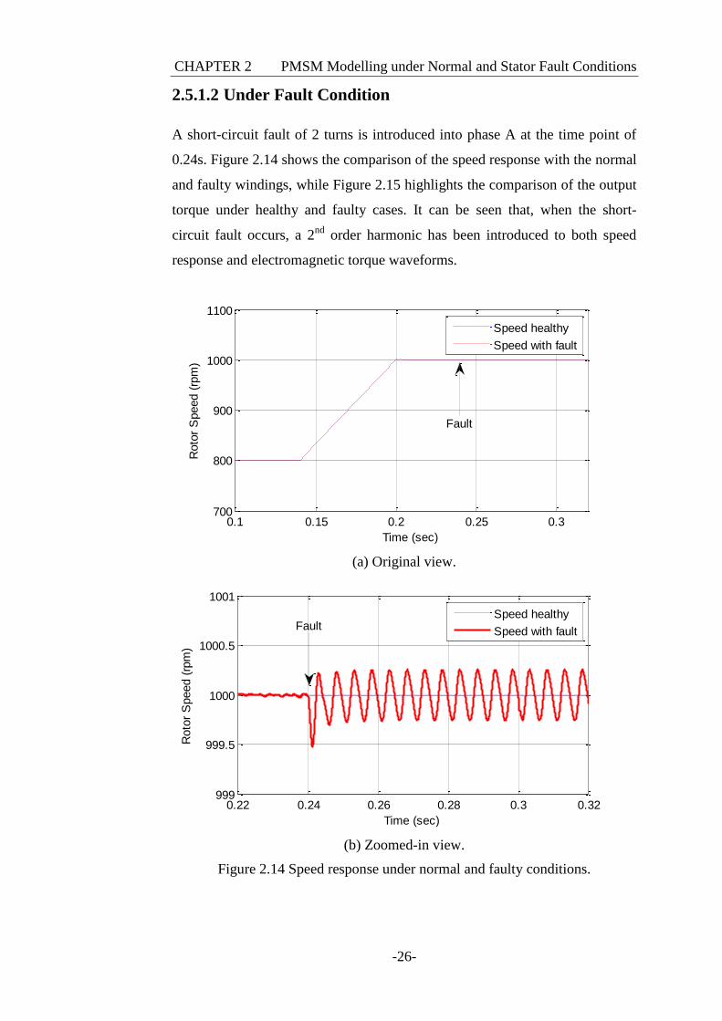
A short-circuit fault of 2 turns is introduced into phase A at the time point of
0.24s. Figure 2.14 shows the comparison of the speed response with the normal
and faulty windings, while Figure 2.15 highlights the comparison of the output
torque under healthy and faulty cases. It can be seen that, when the short-
circuit fault occurs, a 2nd
order harmonic has been introduced to both speed
response and electromagnetic torque waveforms.
(a) Original view.
(b) Zoomed-in view.
Figure 2.14 Speed response under normal and faulty conditions.
0.1 0.15 0.2 0.25 0.3700
800
900
1000
1100
Time (sec)
Roto
r S
peed (
rpm
)
Speed healthy
Speed with fault
Fault
0.22 0.24 0.26 0.28 0.3 0.32999
999.5
1000
1000.5
1001
Time (sec)
Roto
r S
peed (
rpm
)
Speed healthy
Speed with faultFault
CHAPTER 2 PMSM Modelling under Normal and Stator Fault Conditions
-27-
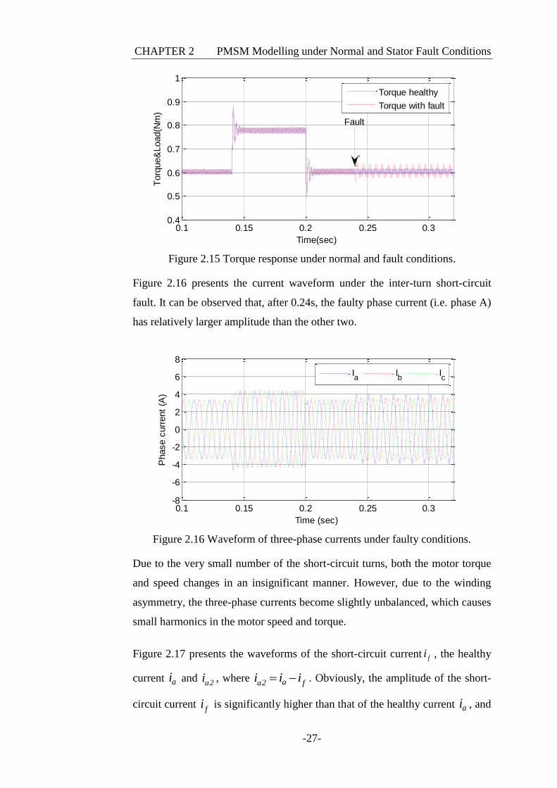
Figure 2.15 Torque response under normal and fault conditions.
Figure 2.16 presents the current waveform under the inter-turn short-circuit
fault. It can be observed that, after 0.24s, the faulty phase current (i.e. phase A)
has relatively larger amplitude than the other two.
Figure 2.16 Waveform of three-phase currents under faulty conditions.
Due to the very small number of the short-circuit turns, both the motor torque
and speed changes in an insignificant manner. However, due to the winding
asymmetry, the three-phase currents become slightly unbalanced, which causes
small harmonics in the motor speed and torque.
Figure 2.17 presents the waveforms of the short-circuit current fi , the healthy
current ai and a2i , where aa2 fi i i . Obviously, the amplitude of the short-
circuit current fi is significantly higher than that of the healthy current ai , and
0.1 0.15 0.2 0.25 0.30.4
0.5
0.6
0.7
0.8
0.9
1
Time(sec)
Torq
ue&
Load(N
m)
Torque healthy
Torque with fault
Fault
0.1 0.15 0.2 0.25 0.3-8
-6
-4
-2
0
2
4
6
8
Time (sec)
Phase c
urr
ent
(A)
Ia
Ib
Ic
CHAPTER 2 PMSM Modelling under Normal and Stator Fault Conditions
-28-
the direction of a2i is opposite to other two currents. The peak value of ai is
3.3A and the peak value of fi is around 21A. The fault current simulation
result is good match with the theoretical. Consequently, a torque is generated,
which resists the output torque resulting in the 2nd
harmonics when the system
is under turn-to-turn short-circuit conditions.
Figure 2.17 Current waveform in phase A winding under faulty conditions.
In order to examine the simulation result presented above, the analytical model
discussed in Section 2.4 can be used for verification. Equation (2.23) lists
system parameters under steady state.
L
1
t
Speed=1000 rpm;
R=0.5 ;
L=3.5 mH;
T 0.6 Nm;
K 1.77 10 Nm/A.
(2.23)
Based on the three-phase PMSM parameters, the back-emf and torque can be
calculated by using (2.2) and (2.11).
E(Peak)=6.78V;
I(Peak)=3.3A; (2.24)
With the short-circuit fault of two turns, the fault current fi can calculated as
follows,
0.2 0.22 0.24 0.26 0.28 0.3 0.32-40
-20
0
20
40
Time (sec)
Phase c
urr
ent
(A)
Ia
If
Ia2
Fault
CHAPTER 2 PMSM Modelling under Normal and Stator Fault Conditions
-29-
2
a.rated
a.ratedf _ Peak
f
V ( E RI ) ( LI ) 10.48V (Peak)
V 10.48i 20.79A(Peak)
R j L 0.5+j0.0608
(2.25)
As it can be seen, a very good match between the theoretical analysis and
simulation results has been demonstrated, which proves the accuracy of the
PMSM modelling under inter-turn faults.
2.5.2 Load Change
For this test, the speed reference of the PMSM motor is fixed at 1000rpm,
while a step change in load will be employed to test the motor performance.
2.5.2.1 Under Healthy Condition
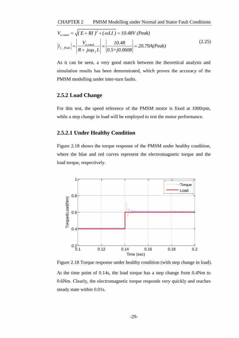
Figure 2.18 shows the torque response of the PMSM under healthy condition,
where the blue and red curves represent the electromagnetic torque and the
load torque, respectively.
Figure 2.18 Torque response under healthy condition (with step change in load).
At the time point of 0.14s, the load torque has a step change from 0.4Nm to
0.6Nm. Clearly, the electromagnetic torque responds very quickly and reaches
steady state within 0.01s.
0.1 0.12 0.14 0.16 0.18 0.20.2
0.4
0.6
0.8
1
Time (sec)
Torq
ue&
Load(N
m)
Torque
Load
CHAPTER 2 PMSM Modelling under Normal and Stator Fault Conditions
-30-
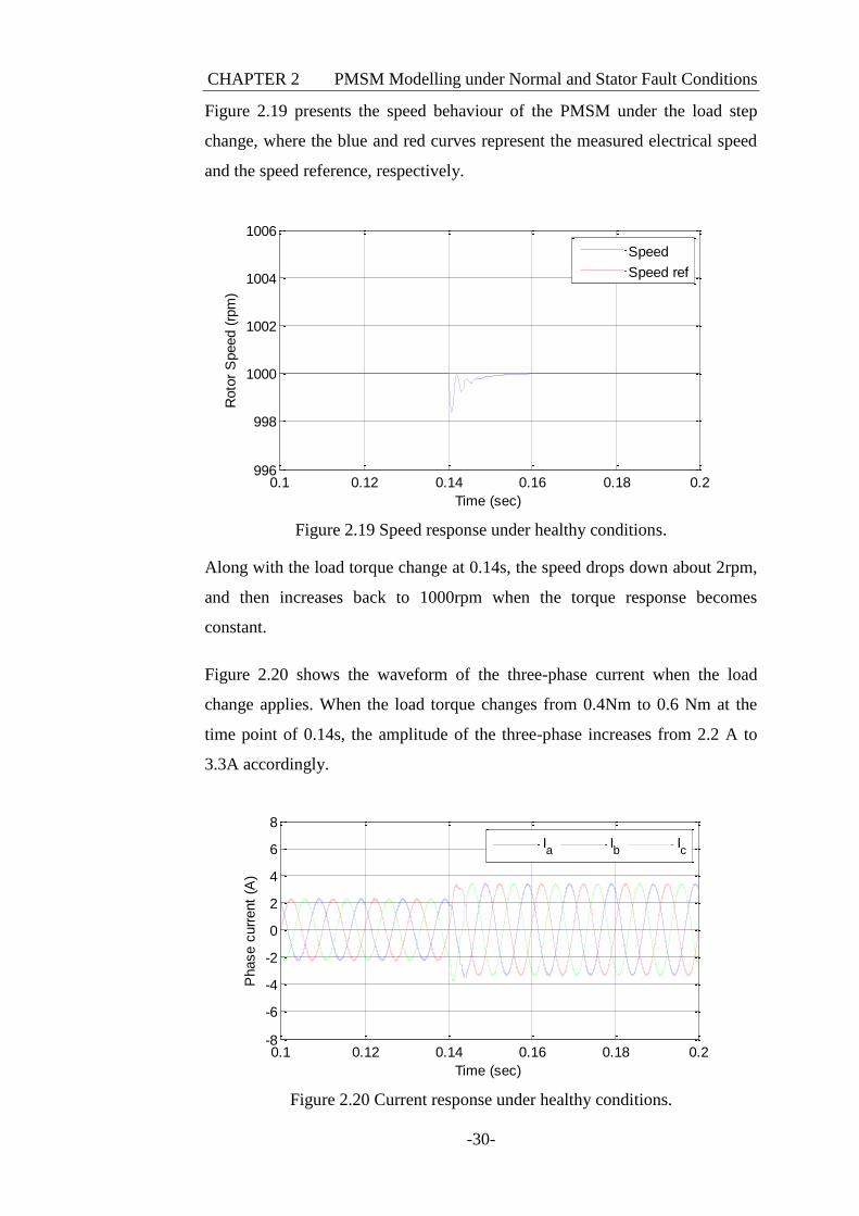
Figure 2.19 presents the speed behaviour of the PMSM under the load step
change, where the blue and red curves represent the measured electrical speed
and the speed reference, respectively.
Figure 2.19 Speed response under healthy conditions.
Along with the load torque change at 0.14s, the speed drops down about 2rpm,
and then increases back to 1000rpm when the torque response becomes
constant.
Figure 2.20 shows the waveform of the three-phase current when the load
change applies. When the load torque changes from 0.4Nm to 0.6 Nm at the
time point of 0.14s, the amplitude of the three-phase increases from 2.2 A to
3.3A accordingly.
Figure 2.20 Current response under healthy conditions.
0.1 0.12 0.14 0.16 0.18 0.2996
998
1000
1002
1004
1006
Time (sec)
Roto
r S
peed (
rpm
)
Speed
Speed ref
0.1 0.12 0.14 0.16 0.18 0.2-8
-6
-4
-2
0
2
4
6
8
Time (sec)
Phase c
urr
ent
(A)
Ia
Ib
Ic
CHAPTER 2 PMSM Modelling under Normal and Stator Fault Conditions
-31-
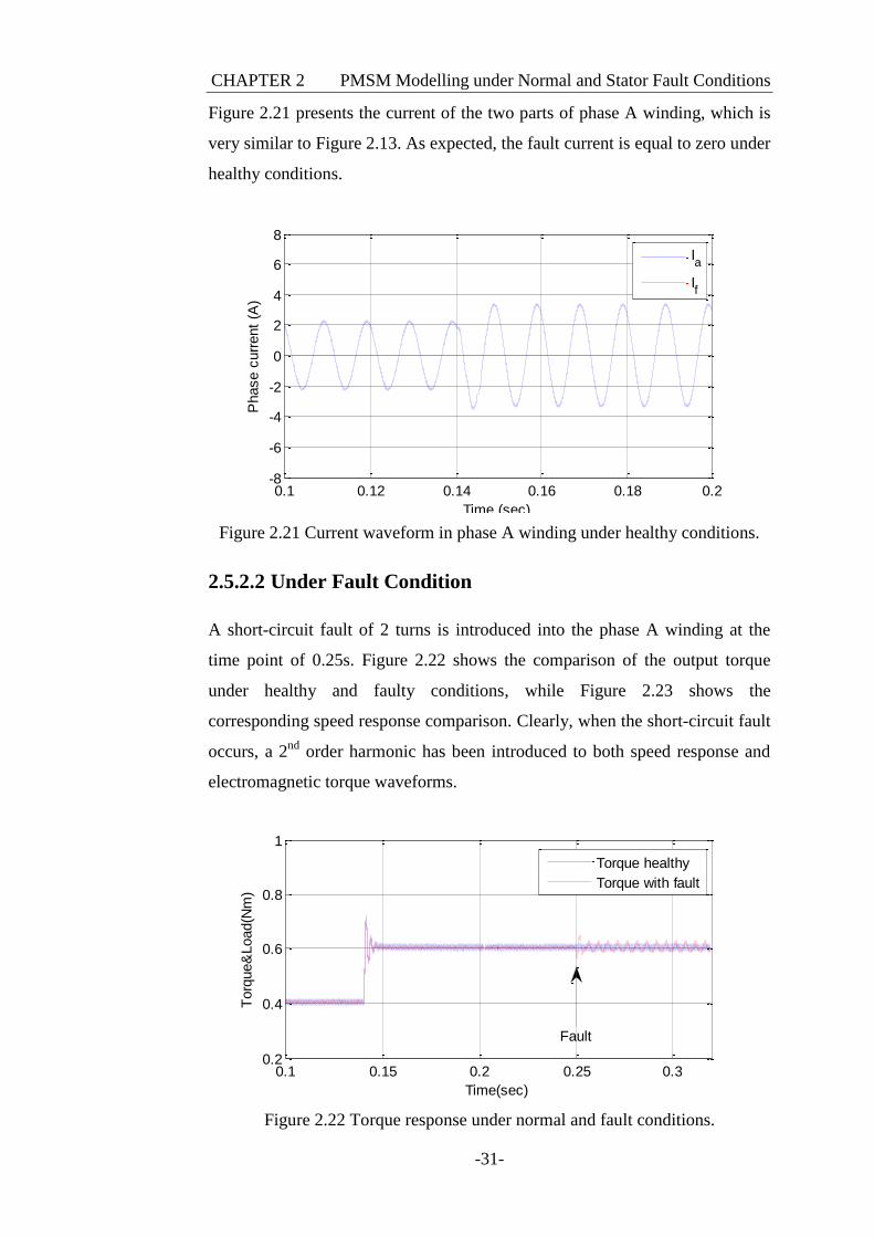
Figure 2.21 presents the current of the two parts of phase A winding, which is
very similar to Figure 2.13. As expected, the fault current is equal to zero under
healthy conditions.
Figure 2.21 Current waveform in phase A winding under healthy conditions.
2.5.2.2 Under Fault Condition
A short-circuit fault of 2 turns is introduced into the phase A winding at the
time point of 0.25s. Figure 2.22 shows the comparison of the output torque
under healthy and faulty conditions, while Figure 2.23 shows the
corresponding speed response comparison. Clearly, when the short-circuit fault
occurs, a 2nd
order harmonic has been introduced to both speed response and
electromagnetic torque waveforms.
Figure 2.22 Torque response under normal and fault conditions.
0.1 0.12 0.14 0.16 0.18 0.2-8
-6
-4
-2
0
2
4
6
8
Time (sec)
Phase c
urr
ent
(A)
Ia
If
0.1 0.15 0.2 0.25 0.30.2
0.4
0.6
0.8
1
Time(sec)
Torq
ue&
Load(N
m)
Torque healthy
Torque with fault
Fault
CHAPTER 2 PMSM Modelling under Normal and Stator Fault Conditions
-32-
Figure 2.23 Speed response under normal and fault conditions.
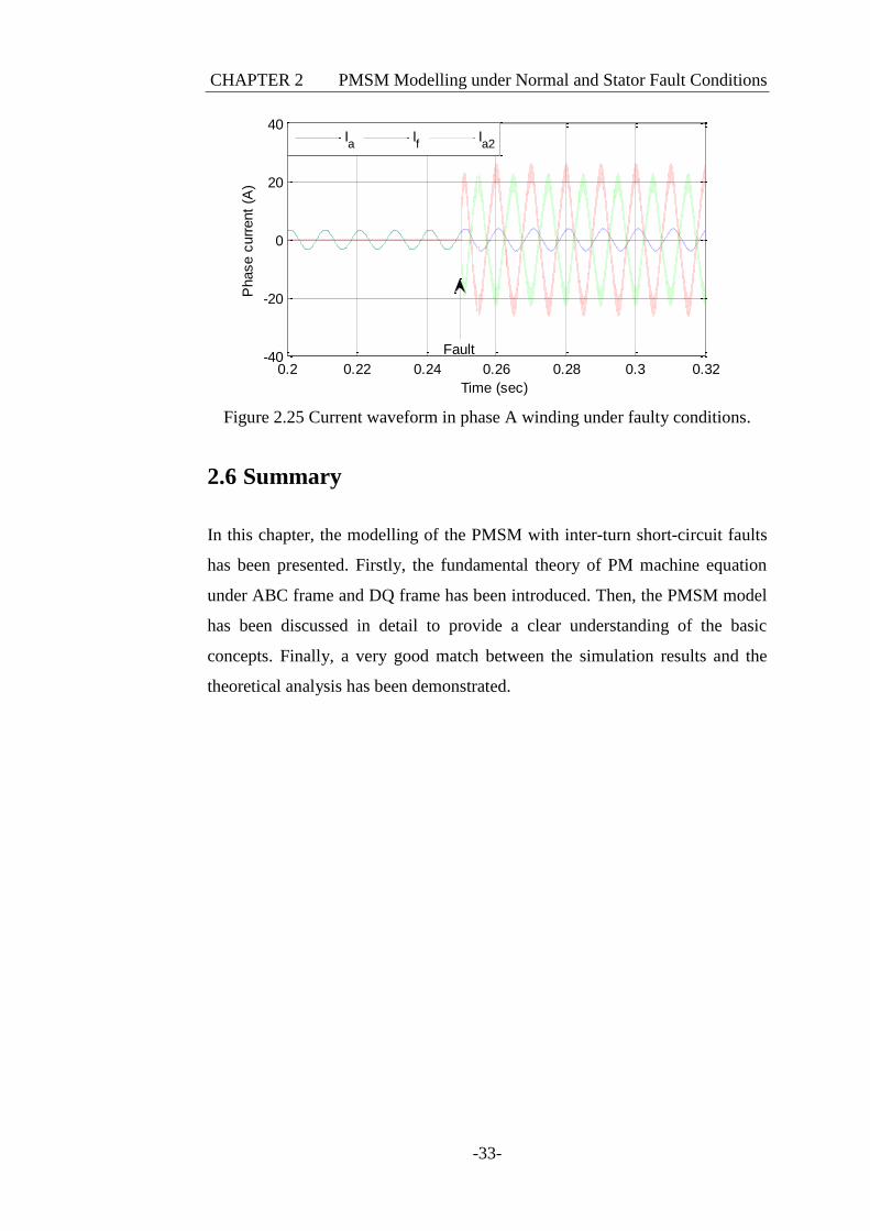
Figure 2.24 shows the waveform of the three-phase current under the short-
circuit fault. When the fault occurs at 0.25s, the amplitude of the faulty phase
current increases a bit.
Figure 2.24 Waveform of three-phase currents under fault condition.
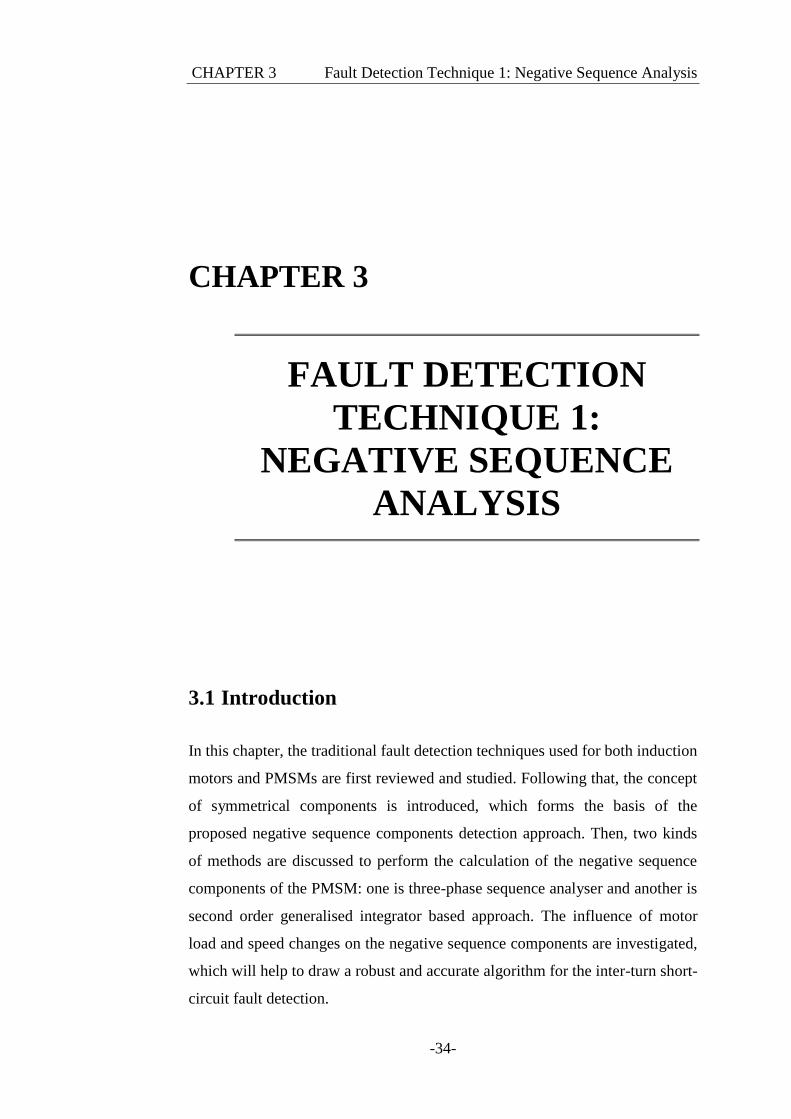
Figure 2.25 presents the waveform of the short-circuit current and the healthy
part current in phase A. The amplitude of the short-circuit current fi is
significantly higher than that of the healthy current, and the direction of a2i is
opposite to other two currents. The fault current value calculated by (2.19) is
20.79A, which is very close the simulation result 21A.
0.22 0.24 0.26 0.28 0.3 0.32999
999.5
1000
1000.5
1001
Time (sec)
Roto
r S
peed (
rpm
)
Speed healthy
Speed with faultFault
0.1 0.15 0.2 0.25 0.3
-5
0
5
Time (sec)
Phase c
urr
ent
(A)
Ia
Ib
Ic
Fault
CHAPTER 2 PMSM Modelling under Normal and Stator Fault Conditions
-33-
Figure 2.25 Current waveform in phase A winding under faulty conditions.
2.6 Summary
In this chapter, the modelling of the PMSM with inter-turn short-circuit faults
has been presented. Firstly, the fundamental theory of PM machine equation
under ABC frame and DQ frame has been introduced. Then, the PMSM model
has been discussed in detail to provide a clear understanding of the basic
concepts. Finally, a very good match between the simulation results and the
theoretical analysis has been demonstrated.
0.2 0.22 0.24 0.26 0.28 0.3 0.32-40
-20
0
20
40
Time (sec)
Phase c
urr
ent
(A)
Ia
If
Ia2
Fault
CHAPTER 3 Fault Detection Technique 1: Negative Sequence Analysis
-34-
CHAPTER 3
FAULT DETECTION
TECHNIQUE 1:
NEGATIVE SEQUENCE
ANALYSIS
3.1 Introduction
In this chapter, the traditional fault detection techniques used for both induction
motors and PMSMs are first reviewed and studied. Following that, the concept
of symmetrical components is introduced, which forms the basis of the
proposed negative sequence components detection approach. Then, two kinds
of methods are discussed to perform the calculation of the negative sequence
components of the PMSM: one is three-phase sequence analyser and another is
second order generalised integrator based approach. The influence of motor
load and speed changes on the negative sequence components are investigated,
which will help to draw a robust and accurate algorithm for the inter-turn short-
circuit fault detection.
CHAPTER 3 Fault Detection Technique 1: Negative Sequence Analysis
-35-
3.2 Fault Detection Techniques
3.2.1 Fault Detection for Induction Motors
Motor current signature analysis (MCSA) is one of the most common
approaches for the fault detection of induction motors [18, 43-45]. By applying
signal processing algorithms, the MCSA analyses motor current waveforms
and can provide early machine diagnosis and protection. However, it requires
long computation time, due to the complexity in mathematics.
Due to the interaction between electrical and mechanical behaviour, inter-turn
faults and some unbalanced electrical faults of induction motors can be
reflected by vibration phenomenon [46, 47]. Based on the measurement of such
signals, vibration signature analysis (VSA) analyses and identifies possible
faults of inductor motors. The main drawbacks of this approach are that.it
demands a number of measurement sensors, which is costly, and is sensitive to
environment noises.
It has been shown that the use of axial flux (AX) is able to reveal magnetic
circuit imbalances [48-50]. Based on this, different methods have been
proposed for AX analysis, in order to diagnose motor faults. Theoretically, a
perfectly balanced machine should have an axial flux of zero. However, small
asymmetries always exist in practice, due to physical discrepancies of stator
windings; for example, this fact implies that any motor will have a small but
non-negligible axial leakage flux, and so this approach demands special care to
obtain reliable data.
Apart from aforementioned methods, many other approaches have been
reported in literature for the fault detection of the induction motor, e.g., thermal
monitoring, gas in oil analysis [11, 15, 29]. However, since this research work
focuses on the diagnosis of short-circuit faults of the PMSM, they are beyond
the scope of this study and will not be discussed here.
CHAPTER 3 Fault Detection Technique 1: Negative Sequence Analysis
-36-
3.2.2 Fault Detection Technique for PMSMs
Generally, faults in PMSMs can be divided into three categories, which are
electrical, magnetic and mechanical faults, respectively [15, 51]. For electrical
faults, it mainly includes abnormal connection of the stator windings, stator
open turns and short-circuit turns etc [41]. Magnetic faults consist of partial or
total demagnetization of the rotor magnets. Mechanical faults cover bearing
and eccentricity faults, (while the latter one further involves static eccentricity,
dynamic eccentricity and mixed eccentricity [51]). The eccentricity faults are
mainly caused by the manufacturing imperfections and imprecision, and can
lead to magnetic and dynamic problems of the PMSM [51]. Since this research
work is dedicated to the inter-turn short-circuit failures, some principal fault
detection techniques are introduced as follows.
Based on the sequence components of the stator current, Reference [52] has
demonstrated an approach to the detection of open-circuit faults in multi-phase
PMSM drives. By using the second-order generalized integrator (SOGI) for the
generation of the quadrature signal, the fundamental negative sequence current
can be evaluated. The Cumulative Sum (CUSUM) algorithm was adopted to
define the decision criterion.
In [53], the author proposed a simplified on-line short-circuit fault detection
scheme for interior permanent magnets synchronous machines (IPMSM), by
looking at a change in positive sequence component supplied by a current-
controlled voltage source inverter (CCVSI). According to the difference
between the DQ axis voltage reference in the look-up table and the actual
voltage references output from the current controller, the fault can be indicated
without using any voltage sensor.
Wavelet transformation has been employed in [21] to diagnose the inter-turn
short-circuit faults of PMSMs. The harmonic components of the stator current
are analysed and transformed into the DQ axis, and the wavelet approach is
applied to extend the analysis to transitory failures.
In this research work, a novel fault detection scheme is presented to assess the
inter-turn short-circuit fault of the PMSMs. The proposed technique is based on
CHAPTER 3 Fault Detection Technique 1: Negative Sequence Analysis
-37-
the negative sequence components of stator currents and impedances, which
will be discussed in the following sections.
3.3 Symmetrical Components
The method of symmetrical components was first proposed by C. L. Fortescue
[54] in 1918. It states that any unbalanced n-phase quantities, i.e. either voltage,
current or impedance, can be represented by n symmetrical sets of balanced
phasors. For example, considering an unbalanced three-phase system shown in
Figure 3.1, each of the three phasors is displaced 120 degrees from the others
in a clockwise rotation sequence.
According to Fortescue’s methodology, for this given system, there are three
sets of independent components: positive, negative and zero sequence
quantities. The positive sequence quantities have the same phase sequence as
the three-phase system. The negative sequence quantities are displaced 120
degrees from the others, but in a counter-clockwise rotation sequence (i.e. A-C-
B). The zero sequence quantities are equal in magnitude in phase with each
other but have no rotation sequence [54].
Va
Vb
Vc
Original
system
Va1
Vb1
Vc1
Positive
sequence
Va2
Vb2
Vc2
Negative
sequence
Va0,Vb0,Vc0Zero
sequence
Figure 3.1 Symmetrical components of unbalanced three-phase system.
CHAPTER 3 Fault Detection Technique 1: Negative Sequence Analysis
-38-
The symmetrical components can be used as an effective tool to determine any
unbalanced variables (e.g. current or voltage) as in (3.1),
0 0
a a
2 0 2 0
b b
2 0 2 0
c c
j2 3
I I I I V V V V
I I I I V V V V
I I I I V V V V
e
(3.1)
where Va, Vb and Vc represent the three-phase unbalanced line to neutral
voltages; Ia, Ib and Ic are the phase current of the three windings; V+, V
- and V
0
are the positive, negative and zero sequence components of the voltage; I+, I
-
and I0 are the positive, negative and zero sequence components of the current;
the α operator shifts a vector by an angle of 120 degrees anti-clockwise, and
the α2 operator performs a 240 degrees counter-clockwise phase shift.
By using (3.1), the symmetrical components of the current and voltage for the
unbalanced three-phase system can be calculated as below,
2 2
a b c a b c
2 2
a b c a b c
0 0
a b c a b c
2
1 1I ( I I I ) V (V V V )
3 3
1 1I ( I I I ) V (V V V )
3 3
1 1I ( I I I ) V (V V V )
3 3
1+ 0
(3.2)
Then, the symmetrical component set can be written as in (3.3), where the
variable x can be either current or voltage.
2
a
2
b
0
c
x 1 x1
x 1 x3
x 1 1 1 x
(3.3)
Following this, the negative sequence impedance can be defined and calculated,
as shown in [46, 55] (3.4),
VZ
I
(3.4)
CHAPTER 3 Fault Detection Technique 1: Negative Sequence Analysis
-39-
In the following sections, the concept of symmetrical components will be
utilised to diagnose the inter-turn short-circuit faults of the PMSM.
3.4 Three-phase Sequence Analyser
3.4.1 General Structure
In this section, the three-phase sequence analyser provided by MatLab-
Simulink is utilised to calculate the negative sequence components. For a
specified frequency, this block first applies a Fourier analysis over a sliding
window of one cycle of the three input signals. Then, it evaluates the phasors
values and derives the positive sequence, negative sequence, and zero sequence.
Figure 3.2 shows the block diagram of a three-phase sequence analyser for
negative sequence components calculation. It should be pointed out that, due to
the use of the sliding window for the Fourier transformation, one cycle of
simulation has to be completed before the outputs give the correct magnitude
and angle. Consequently, the evaluation of the symmetrical components is
always delayed by one cycle of the fundamental frequency. The calculation
procedure of the sequence components can be found in (3.3).
Figure 3.2 Block diagram of three-phase sequence analyser for negative
sequence components calculation.
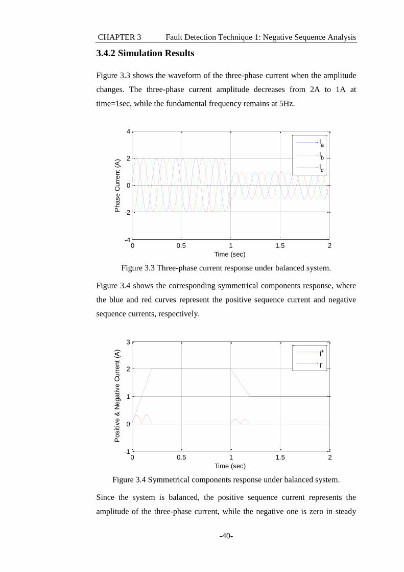
CHAPTER 3 Fault Detection Technique 1: Negative Sequence Analysis
-40-
3.4.2 Simulation Results
Figure 3.3 shows the waveform of the three-phase current when the amplitude
changes. The three-phase current amplitude decreases from 2A to 1A at
time=1sec, while the fundamental frequency remains at 5Hz.
Figure 3.3 Three-phase current response under balanced system.
Figure 3.4 shows the corresponding symmetrical components response, where
the blue and red curves represent the positive sequence current and negative
sequence currents, respectively.
Figure 3.4 Symmetrical components response under balanced system.
Since the system is balanced, the positive sequence current represents the
amplitude of the three-phase current, while the negative one is zero in steady
0 0.5 1 1.5 2-4
-2
0
2
4
Time (sec)
Phase C
urr
ent
(A)
Ia
Ib
Ic
0 0.5 1 1.5 2-1
0
1
2
3
Time (sec)
Positiv
e &
Negative C
urr
ent
(A)
I+
I-
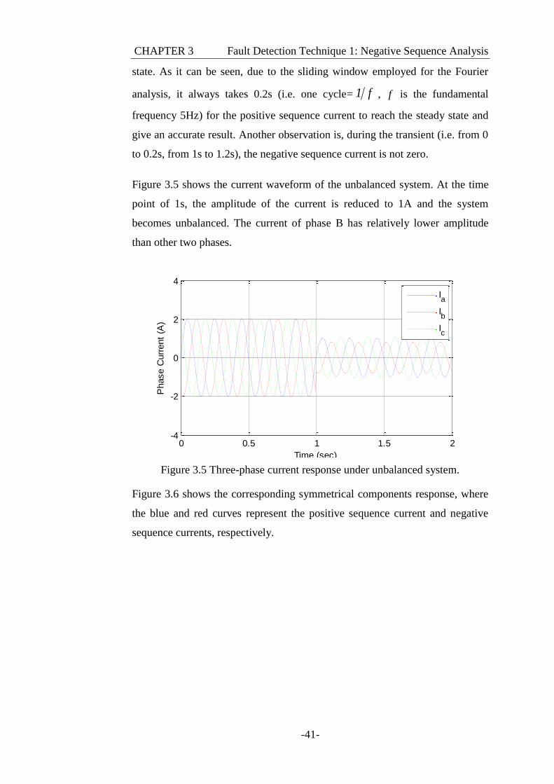
CHAPTER 3 Fault Detection Technique 1: Negative Sequence Analysis
-41-
state. As it can be seen, due to the sliding window employed for the Fourier
analysis, it always takes 0.2s (i.e. one cycle= 1 f , f is the fundamental
frequency 5Hz) for the positive sequence current to reach the steady state and
give an accurate result. Another observation is, during the transient (i.e. from 0
to 0.2s, from 1s to 1.2s), the negative sequence current is not zero.
Figure 3.5 shows the current waveform of the unbalanced system. At the time
point of 1s, the amplitude of the current is reduced to 1A and the system
becomes unbalanced. The current of phase B has relatively lower amplitude
than other two phases.
Figure 3.5 Three-phase current response under unbalanced system.
Figure 3.6 shows the corresponding symmetrical components response, where
the blue and red curves represent the positive sequence current and negative
sequence currents, respectively.
0 0.5 1 1.5 2-4
-2
0
2
4
Time (sec)
Phase C
urr
ent
(A)
Ia
Ib
Ic
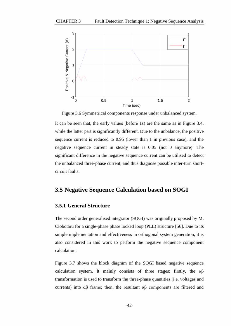
CHAPTER 3 Fault Detection Technique 1: Negative Sequence Analysis
-42-
Figure 3.6 Symmetrical components response under unbalanced system.
It can be seen that, the early values (before 1s) are the same as in Figure 3.4,
while the latter part is significantly different. Due to the unbalance, the positive
sequence current is reduced to 0.95 (lower than 1 in previous case), and the
negative sequence current in steady state is 0.05 (not 0 anymore). The
significant difference in the negative sequence current can be utilised to detect
the unbalanced three-phase current, and thus diagnose possible inter-turn short-
circuit faults.
3.5 Negative Sequence Calculation based on SOGI
3.5.1 General Structure
The second order generalised integrator (SOGI) was originally proposed by M.
Ciobotaru for a single-phase phase locked loop (PLL) structure [56]. Due to its
simple implementation and effectiveness in orthogonal system generation, it is
also considered in this work to perform the negative sequence component
calculation.
Figure 3.7 shows the block diagram of the SOGI based negative sequence
calculation system. It mainly consists of three stages: firstly, the αβ
transformation is used to transform the three-phase quantities (i.e. voltages and
currents) into αβ frame; then, the resultant αβ components are filtered and
0 0.5 1 1.5 2-1
0
1
2
3
Time (sec)
Positiv
e &
Negative C
urr
ent
(A)
I+
I-
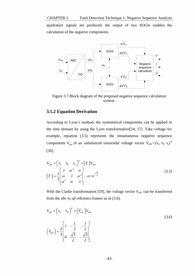
CHAPTER 3 Fault Detection Technique 1: Negative Sequence Analysis
-43-
quadrature signals are produced; the output of two SOGIs enables the
calculation of the negative components.
ABC
DQ
Vabc
Iabc
ωe
SOGI
V/Iα
V/Iβ
SOGI
Negative
sequence
calculation
V’/I’α
qV’/I’α
V’/I’β
qV’/I’β
V -
I -
Z -
Figure 3.7 Block diagram of the proposed negative sequence calculation
system.
3.5.2 Equation Derivation
According to Lyon’s method, the symmetrical components can be applied in
the time domain by using the Lyon transformation[54, 57]. Take voltage for
example, equation (3.5) represents the instantaneous negative sequence
components abcV of an unbalanced sinusoidal voltage vector Vabc=[va vb vc]
T
[58].
T
abc a b c abc
2
2j
2 3
2
V v v v T V
11
T 1 , =e3
1
(3.5)
With the Clarke transformation [59], the voltage vector Vabc can be transferred
from the abc to αβ reference frames as in (3.6).
T
abcV v v T V
1 11
2 2 2T
3 3 30
2 2
(3.6)
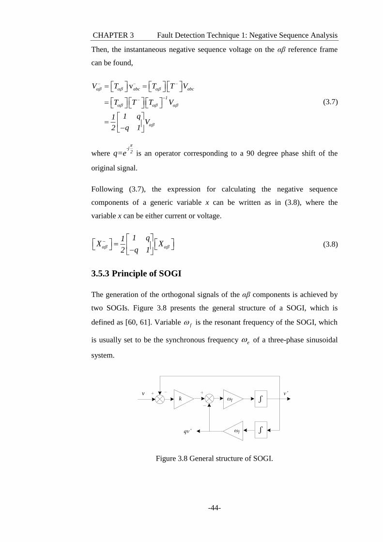
CHAPTER 3 Fault Detection Technique 1: Negative Sequence Analysis
-44-
Then, the instantaneous negative sequence voltage on the αβ reference frame
can be found,
vabc abc
1
V T T T V
T T T V
1 q1 V
q 12
(3.7)
where
π-j
2q=e is an operator corresponding to a 90 degree phase shift of the
original signal.
Following (3.7), the expression for calculating the negative sequence
components of a generic variable x can be written as in (3.8), where the
variable x can be either current or voltage.
1 q1X X
q 12
(3.8)
3.5.3 Principle of SOGI
The generation of the orthogonal signals of the αβ components is achieved by
two SOGIs. Figure 3.8 presents the general structure of a SOGI, which is
defined as [60, 61]. Variable f is the resonant frequency of the SOGI, which
is usually set to be the synchronous frequency e of a three-phase sinusoidal
system.
vk
qv’
ωf ʃ
ωf ʃ
v’
Figure 3.8 General structure of SOGI.
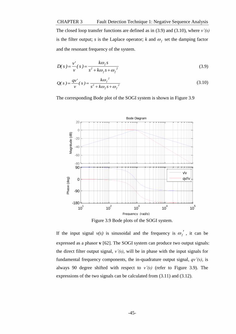
CHAPTER 3 Fault Detection Technique 1: Negative Sequence Analysis
-45-
The closed loop transfer functions are defined as in (3.9) and (3.10), where v’(s)
is the filter output; s is the Laplace operator; k and f set the damping factor
and the resonant frequency of the system.
f
2 2
f f
k sv'D( s ) ( s )
v s k s
(3.9)
2
f
2 2
f f
kqv'Q( s ) ( s )
v s k s
(3.10)
The corresponding Bode plot of the SOGI system is shown in Figure 3.9
Figure 3.9 Bode plots of the SOGI system.
If the input signal v(s) is sinusoidal and the frequency is f , it can be
expressed as a phasor v [62]. The SOGI system can produce two output signals:
the direct filter output signal, v’(s), will be in phase with the input signals for
fundamental frequency components, the in-quadrature output signal, qv’(s), is
always 90 degree shifted with respect to v’(s) (refer to Figure 3.9). The
expressions of the two signals can be calculated from (3.11) and (3.12).
-80
-60
-40
-20
0
20
Magnitu
de (
dB
)
101
102
103
104
105
-180
-90
0
90
Phase (
deg)
Bode Diagram
Frequency (rad/s)
v'v
qv'/v
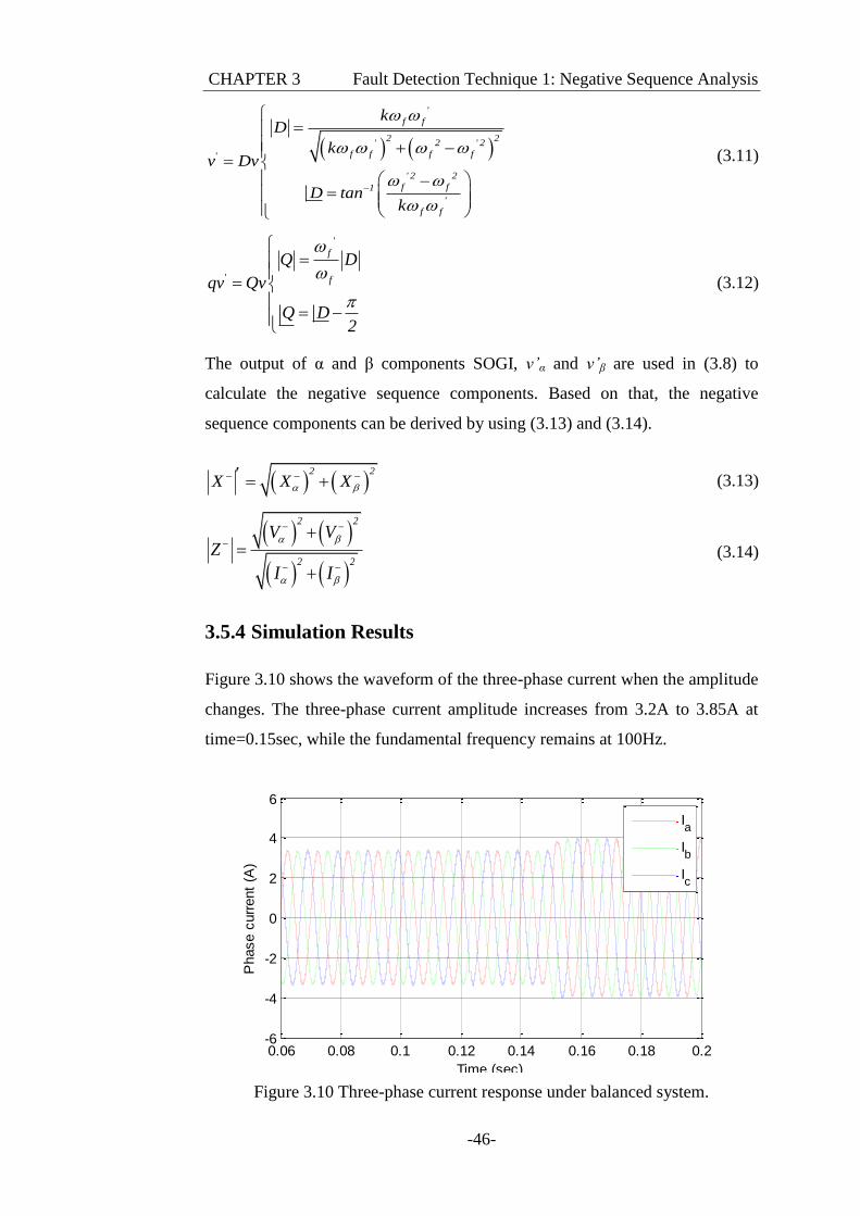
CHAPTER 3 Fault Detection Technique 1: Negative Sequence Analysis
-46-
'
f f
2 2' 2 ' 2
f f f f'
' 2 2
f f1
'
f f
kD
kv Dv
D tank
(3.11)
'
f
' f
Q D
qv Qv
Q D2
(3.12)
The output of α and β components SOGI, v’α and v’β are used in (3.8) to
calculate the negative sequence components. Based on that, the negative
sequence components can be derived by using (3.13) and (3.14).
2 2
X X X (3.13)
2 2
2 2
V VZ
I I
(3.14)
3.5.4 Simulation Results
Figure 3.10 shows the waveform of the three-phase current when the amplitude
changes. The three-phase current amplitude increases from 3.2A to 3.85A at
time=0.15sec, while the fundamental frequency remains at 100Hz.
Figure 3.10 Three-phase current response under balanced system.
0.06 0.08 0.1 0.12 0.14 0.16 0.18 0.2-6
-4
-2
0
2
4
6
Time (sec)
Phase c
urr
ent
(A)
Ia
Ib
Ic
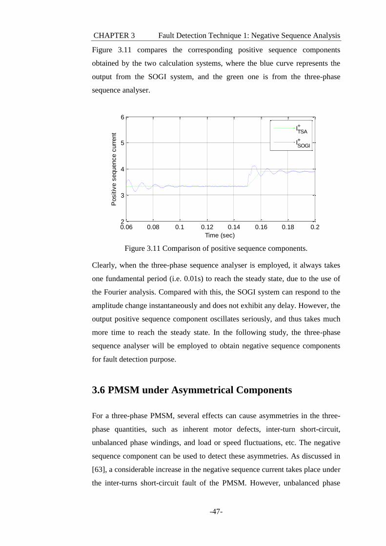
CHAPTER 3 Fault Detection Technique 1: Negative Sequence Analysis
-47-
Figure 3.11 compares the corresponding positive sequence components
obtained by the two calculation systems, where the blue curve represents the
output from the SOGI system, and the green one is from the three-phase
sequence analyser.
Figure 3.11 Comparison of positive sequence components.
Clearly, when the three-phase sequence analyser is employed, it always takes
one fundamental period (i.e. 0.01s) to reach the steady state, due to the use of
the Fourier analysis. Compared with this, the SOGI system can respond to the
amplitude change instantaneously and does not exhibit any delay. However, the
output positive sequence component oscillates seriously, and thus takes much
more time to reach the steady state. In the following study, the three-phase
sequence analyser will be employed to obtain negative sequence components
for fault detection purpose.
3.6 PMSM under Asymmetrical Components
For a three-phase PMSM, several effects can cause asymmetries in the three-
phase quantities, such as inherent motor defects, inter-turn short-circuit,
unbalanced phase windings, and load or speed fluctuations, etc. The negative
sequence component can be used to detect these asymmetries. As discussed in
[63], a considerable increase in the negative sequence current takes place under
the inter-turns short-circuit fault of the PMSM. However, unbalanced phase
0.06 0.08 0.1 0.12 0.14 0.16 0.18 0.22
3
4
5
6
Time (sec)
Positiv
e s
equence c
urr
ent
I+TSA
I+SOGI
CHAPTER 3 Fault Detection Technique 1: Negative Sequence Analysis
-48-
windings (i.e. back-emf unbalanced) can produce a similar asymmetry. In order
to produce an accurate and robust fault detection system, some modifications to
this approach are needed.
In this section, the negative sequence analysis based approach is applied to
diagnose inter-turn short-circuit faults of the PMSM. Based on the
measurement of the voltage and current variables, the negative sequence
components of the system are calculated by using the three-phase sequence
analyser. Meanwhile, the PMSM drive is tested with either speed or load
fluctuations, in order to obtain the behaviour of the negative components,
under such conditions.
3.6.1 Speed Fluctuation
In this sub-section, the PMSM motor is set to supply a constant load of 0.6Nm,
with 2% asymmetrical components of back-emf in the phase A. The speed
reference ramps up and down between 800 rpm and 1000rpm, as Figure 3.12
shows, in order to give a complete performance test under speed fluctuation. A
short-circuit fault of 2 turns is injected into phase A time = 0.5s.
Figure 3.12 PMSM speed response under speed fluctuation test.
Figure 3.13 presents the corresponding negative sequence current under this
testing condition. As can be noticed, although the inter-turn short-circuit fault
can be revealed immediately after its occurrence, six false alarms are also
0.1 0.2 0.3 0.4 0.5 0.6700
800
900
1000
1100
Time (sec)
Roto
r S
peed (
rpm
)
Speed reference
Speed with fault
CHAPTER 3 Fault Detection Technique 1: Negative Sequence Analysis
-49-
generated at 0.14s, 0.2s, 0.25, 0.3, 0.35 and 0.4, whose values are almost higher
than that of the real fault conditions.
Figure 3.13 Negative sequence current under speed fluctuation and fault
conditions.
Obviously, these six false alarms are caused by the speed fluctuation. When a
speed change occurs, it brings a non-stationary symmetry condition which
generates a considerable increment on the magnitude of the negative sequence
current. As a result, a false alarm may arise in the detection system.
Figure 3.14 shows the corresponding negative sequence impedance under this
testing condition. Similarly, the negative sequence impedance fluctuates
signicantly during the speed change of the PMSM.
Figure 3.14 Negative sequence impedance under speed fluctuation and fault
conditions.
0.1 0.2 0.3 0.4 0.5 0.6-0.2
-0.1
0
0.1
0.2
0.3
0.4
Time (sec)
Negative S
equence C
urr
ent
(A)
False AlarmFalse Alarm
Fault
0.1 0.2 0.3 0.4 0.5 0.60
2
4
6
8
Time (sec)
Negative S
equence I
mpedance
Fault
Speed Fluctuation Speed Fluctuation
CHAPTER 3 Fault Detection Technique 1: Negative Sequence Analysis
-50-
Obviously, using this information only will lead to a false alarm, so some
filtering algorithm is required to remove the false alarms.
Figure 3.15 shows the waveform of the negative sequence current, when a
moving average filter is utilised for signal processing.
Figure 3.15 Negative sequence current with moving average filter under speed
fluctuation and fault condition.
In this case, the moving average filter has averaged the high frequency
component produced by the speed change over half cycle, as shown in Figure
3.16. The negative sequence current still experiences a high value either under
speed fluctuation or the inter-turn short-circuit fault, though the waveform
becomes much smoother, and the time constant of false alarm= 2 , is
the electrical angular speed (refer to section 3.4.2).
Figure 3.16 Block diagram of moving average filter.
0.1 0.2 0.3 0.4 0.5 0.6-0.2
-0.1
0
0.1
0.2
0.3
0.4
Time (sec)
Negative S
equence C
urr
ent
(A)
1
OutputTi
1
s
1/2
2
Frequency
1
Input
CHAPTER 3 Fault Detection Technique 1: Negative Sequence Analysis
-51-
Figure 3.17 gives the corresponding waveform of the negative sequence
impedance, when the moving average filter is employed. As it can be noticed,
the negative sequence impedance experiences a considerable increase when the
speed changes. In contrast, it drops significantly (i.e. from 2.2 to 1.7) as the
inter-turn short-circuit takes place.
Figure 3.17 Negative sequence impedance with moving average filter under
speed fluctuation and fault condition.
3.6.2 Load fluctuation
In this sub-section, the speed reference of the PMSM motor is fixed at
1000rpm with 2% asymmetrical components set in the back-emf of Phase A. A
step change in load is considered to examine its possible influence on the
negative sequence components.
As shown in Figure 3.18, the load torque steps up and down between 0.4Nm
and 0.6Nm, in order to give a complete performance test under load fluctuation.
A short-circuit fault of 2 turns is introduced into phase A at 0.5s. The blue and
red curves represent the electromagnetic torque and load torque, respectively.
0.1 0.2 0.3 0.4 0.5 0.6
1.5
2
2.5
3
3.5
4
Time (sec)
Negative S
equence I
mpedance
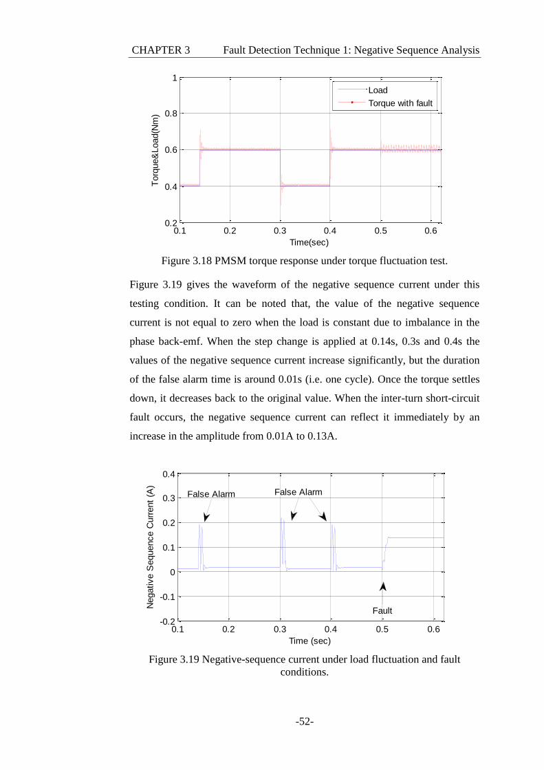
CHAPTER 3 Fault Detection Technique 1: Negative Sequence Analysis
-52-
Figure 3.18 PMSM torque response under torque fluctuation test.
Figure 3.19 gives the waveform of the negative sequence current under this
testing condition. It can be noted that, the value of the negative sequence
current is not equal to zero when the load is constant due to imbalance in the
phase back-emf. When the step change is applied at 0.14s, 0.3s and 0.4s the
values of the negative sequence current increase significantly, but the duration
of the false alarm time is around 0.01s (i.e. one cycle). Once the torque settles
down, it decreases back to the original value. When the inter-turn short-circuit
fault occurs, the negative sequence current can reflect it immediately by an
increase in the amplitude from 0.01A to 0.13A.
Figure 3.19 Negative-sequence current under load fluctuation and fault
conditions.
0.1 0.2 0.3 0.4 0.5 0.60.2
0.4
0.6
0.8
1
Time(sec)
Torq
ue&
Load(N
m)
Load
Torque with fault
0.1 0.2 0.3 0.4 0.5 0.6-0.2
-0.1
0
0.1
0.2
0.3
0.4
Time (sec)
Negative S
equence C
urr
ent
(A)
False Alarm False Alarm
Fault
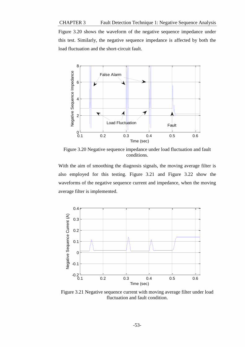
CHAPTER 3 Fault Detection Technique 1: Negative Sequence Analysis
-53-
Figure 3.20 shows the waveform of the negative sequence impedance under
this test. Similarly, the negative sequence impedance is affected by both the
load fluctuation and the short-circuit fault.
Figure 3.20 Negative sequence impedance under load fluctuation and fault
conditions.
With the aim of smoothing the diagnosis signals, the moving average filter is
also employed for this testing. Figure 3.21 and Figure 3.22 show the
waveforms of the negative sequence current and impedance, when the moving
average filter is implemented.
Figure 3.21 Negative sequence current with moving average filter under load
fluctuation and fault condition.
0.1 0.2 0.3 0.4 0.5 0.60
2
4
6
8
Time (sec)
Negative S
equence I
mpedance
False Alarm
FaultLoad Fluctuation
0.1 0.2 0.3 0.4 0.5 0.6-0.2
-0.1
0
0.1
0.2
0.3
0.4
Time (sec)
Negative S
equence C
urr
ent
(A)
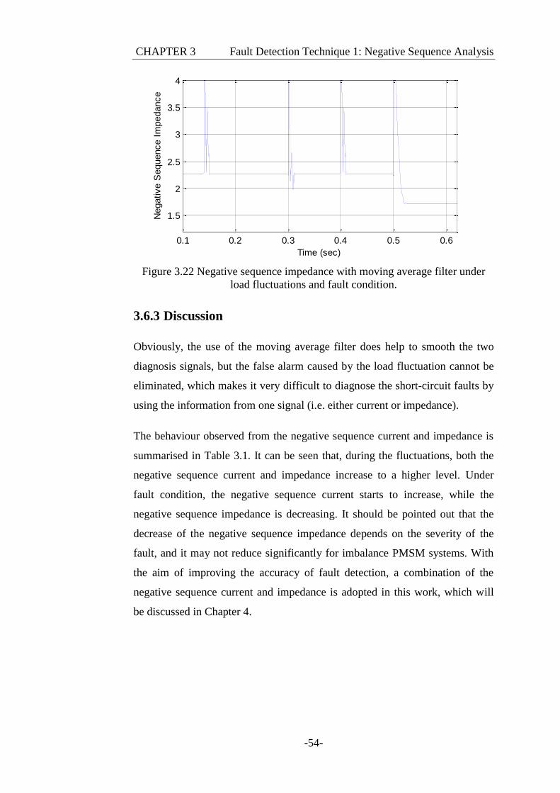
CHAPTER 3 Fault Detection Technique 1: Negative Sequence Analysis
-54-
Figure 3.22 Negative sequence impedance with moving average filter under
load fluctuations and fault condition.
3.6.3 Discussion
Obviously, the use of the moving average filter does help to smooth the two
diagnosis signals, but the false alarm caused by the load fluctuation cannot be
eliminated, which makes it very difficult to diagnose the short-circuit faults by
using the information from one signal (i.e. either current or impedance).
The behaviour observed from the negative sequence current and impedance is
summarised in Table 3.1. It can be seen that, during the fluctuations, both the
negative sequence current and impedance increase to a higher level. Under
fault condition, the negative sequence current starts to increase, while the
negative sequence impedance is decreasing. It should be pointed out that the
decrease of the negative sequence impedance depends on the severity of the
fault, and it may not reduce significantly for imbalance PMSM systems. With
the aim of improving the accuracy of fault detection, a combination of the
negative sequence current and impedance is adopted in this work, which will
be discussed in Chapter 4.
0.1 0.2 0.3 0.4 0.5 0.6
1.5
2
2.5
3
3.5
4
Time (sec)
Negative S
equence I
mpedance
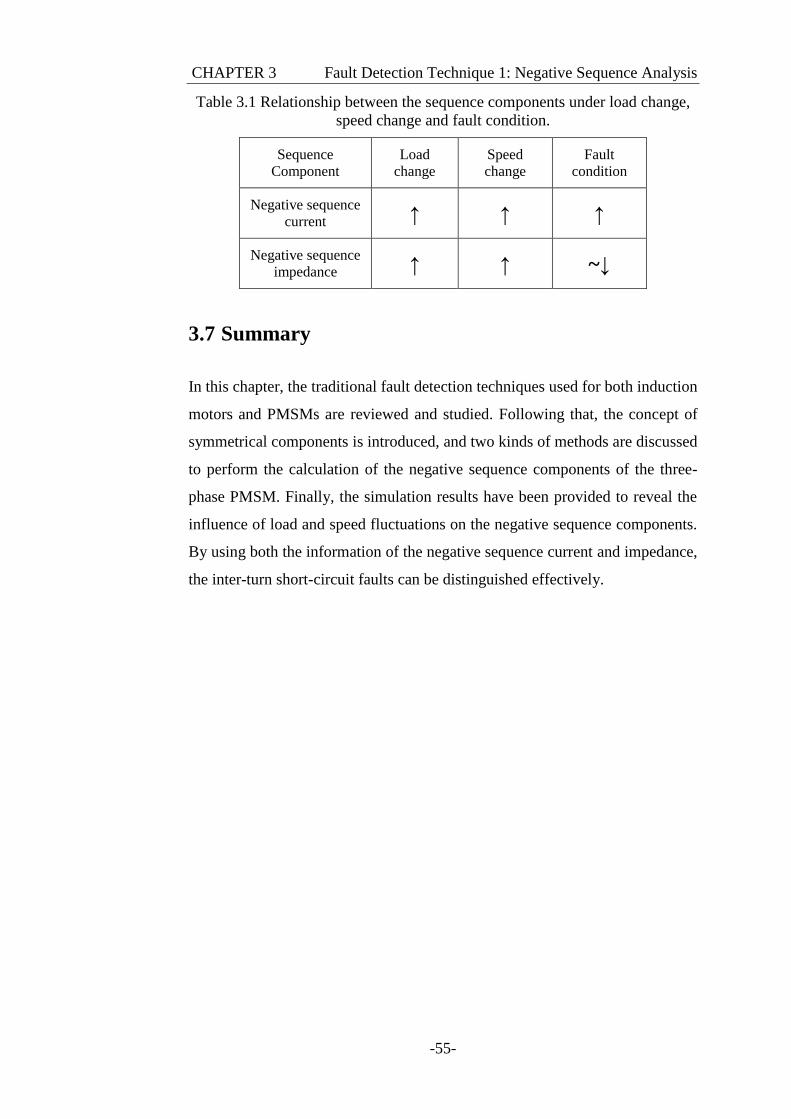
CHAPTER 3 Fault Detection Technique 1: Negative Sequence Analysis
-55-
Table 3.1 Relationship between the sequence components under load change,
speed change and fault condition.
Sequence
Component
Load
change
Speed
change
Fault
condition
Negative sequence
current ↑ ↑ ↑
Negative sequence
impedance ↑ ↑ ~↓
3.7 Summary
In this chapter, the traditional fault detection techniques used for both induction
motors and PMSMs are reviewed and studied. Following that, the concept of
symmetrical components is introduced, and two kinds of methods are discussed
to perform the calculation of the negative sequence components of the three-
phase PMSM. Finally, the simulation results have been provided to reveal the
influence of load and speed fluctuations on the negative sequence components.
By using both the information of the negative sequence current and impedance,
the inter-turn short-circuit faults can be distinguished effectively.
CHAPTER 4 Fault Detection Technique: Fuzzy Logic Approach
-56-
CHAPTER 4
FAULT DETECTION
TECHNIQUE 2: FUZZY
LOGIC APPROACH
4.1 Introduction
Previous research work has demonstrated clearly that, the inter-turn short-
circuit faults can be reflected by using the negative sequence current or
impedance in the system steady state. However, as shown in the simulation
results, the false alarm caused by load or speed fluctuation cannot be
eliminated, which makes it very difficult to diagnose the short-circuit faults by
using the information from one signal only (i.e. either current or impedance).
For this reason, a novel fuzzy logic based approach is considered in this work
for the fault detection of the PMSMs, in order to utilise the information of both
the negative sequence current and impedance to draw a clear and accurate
detection result.
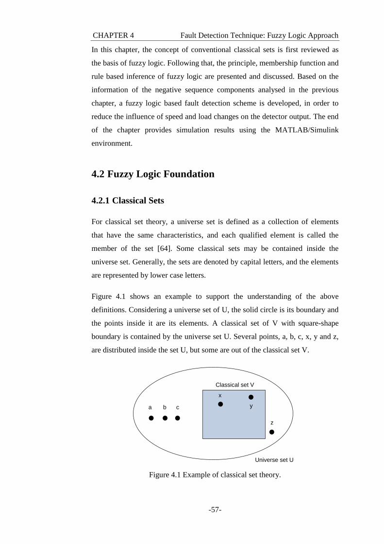
CHAPTER 4 Fault Detection Technique: Fuzzy Logic Approach
-57-
In this chapter, the concept of conventional classical sets is first reviewed as
the basis of fuzzy logic. Following that, the principle, membership function and
rule based inference of fuzzy logic are presented and discussed. Based on the
information of the negative sequence components analysed in the previous
chapter, a fuzzy logic based fault detection scheme is developed, in order to
reduce the influence of speed and load changes on the detector output. The end
of the chapter provides simulation results using the MATLAB/Simulink
environment.
4.2 Fuzzy Logic Foundation
4.2.1 Classical Sets
For classical set theory, a universe set is defined as a collection of elements
that have the same characteristics, and each qualified element is called the
member of the set [64]. Some classical sets may be contained inside the
universe set. Generally, the sets are denoted by capital letters, and the elements
are represented by lower case letters.
Figure 4.1 shows an example to support the understanding of the above
definitions. Considering a universe set of U, the solid circle is its boundary and
the points inside it are its elements. A classical set of V with square-shape
boundary is contained by the universe set U. Several points, a, b, c, x, y and z,
are distributed inside the set U, but some are out of the classical set V.
Universe set U
Classical set V
a b c
x
y
z
Figure 4.1 Example of classical set theory.
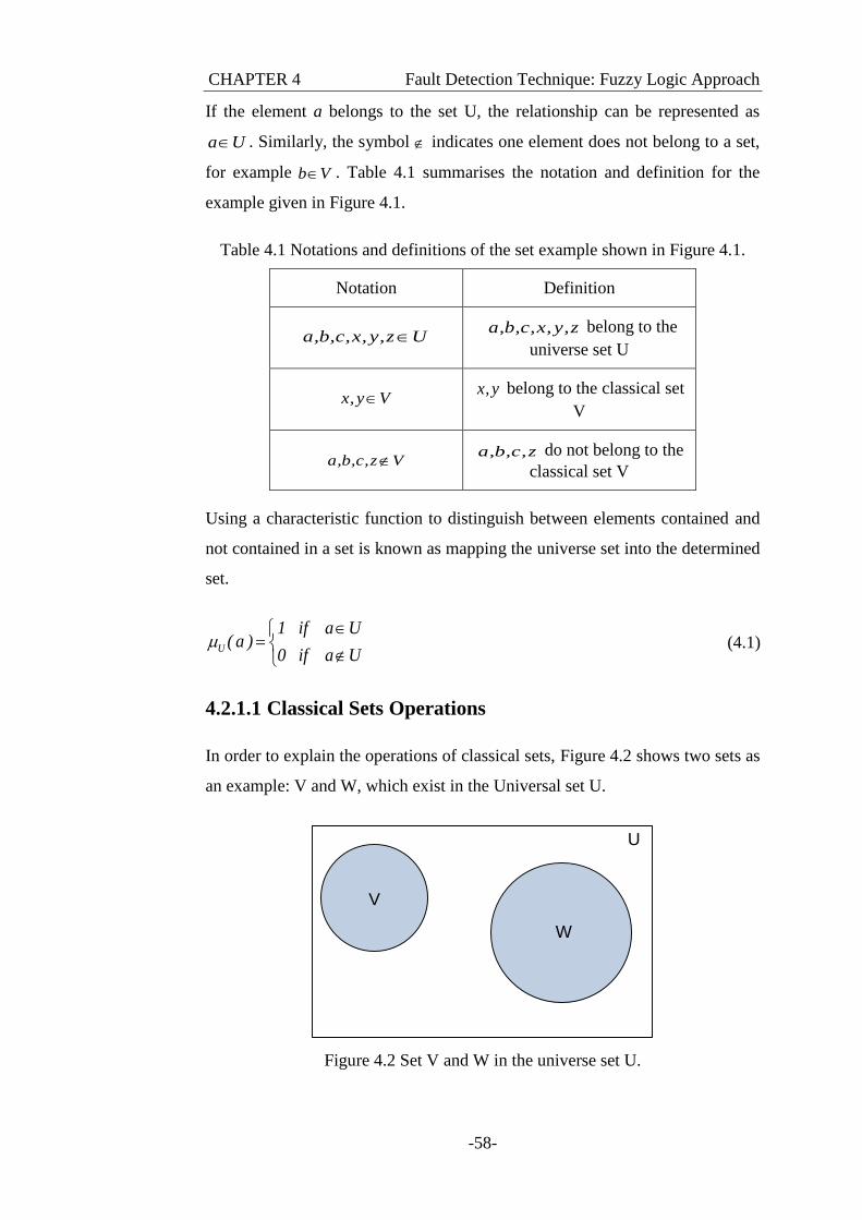
CHAPTER 4 Fault Detection Technique: Fuzzy Logic Approach
-58-
If the element a belongs to the set U, the relationship can be represented as
a U . Similarly, the symbol indicates one element does not belong to a set,
for example b V . Table 4.1 summarises the notation and definition for the
example given in Figure 4.1.
Table 4.1 Notations and definitions of the set example shown in Figure 4.1.
Notation Definition
a,b,c,x, y,z U a,b,c,x, y,z belong to the
universe set U
x, y V x, y belong to the classical set
V
a,b,c,z V a,b,c,z do not belong to the
classical set V
Using a characteristic function to distinguish between elements contained and
not contained in a set is known as mapping the universe set into the determined
set.
U
1 if a U( a )
0 if a U
(4.1)
4.2.1.1 Classical Sets Operations
In order to explain the operations of classical sets, Figure 4.2 shows two sets as
an example: V and W, which exist in the Universal set U.
U
V
W
Figure 4.2 Set V and W in the universe set U.
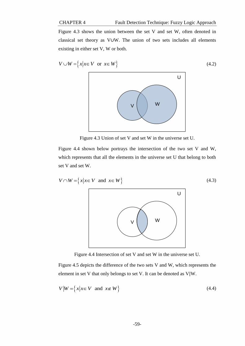
CHAPTER 4 Fault Detection Technique: Fuzzy Logic Approach
-59-
Figure 4.3 shows the union between the set V and set W, often denoted in
classical set theory as V∪W. The union of two sets includes all elements
existing in either set V, W or both.
or V W x x V x W (4.2)
U
V W
Figure 4.3 Union of set V and set W in the universe set U.
Figure 4.4 shown below portrays the intersection of the two set V and W,
which represents that all the elements in the universe set U that belong to both
set V and set W.
and V W x x V x W (4.3)
U
V W
Figure 4.4 Intersection of set V and set W in the universe set U.
Figure 4.5 depicts the difference of the two sets V and W, which represents the
element in set V that only belongs to set V. It can be denoted as V|W.
and V W x x V x W (4.4)
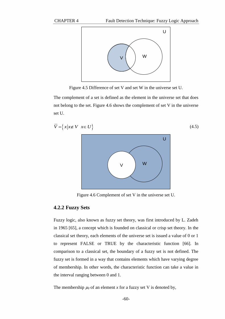
CHAPTER 4 Fault Detection Technique: Fuzzy Logic Approach
-60-
U
WV
Figure 4.5 Difference of set V and set W in the universe set U.
The complement of a set is defined as the element in the universe set that does
not belong to the set. Figure 4.6 shows the complement of set V in the universe
set U.
V x x V x U (4.5)
U
WV
Figure 4.6 Complement of set V in the universe set U.
4.2.2 Fuzzy Sets
Fuzzy logic, also known as fuzzy set theory, was first introduced by L. Zadeh
in 1965 [65], a concept which is founded on classical or crisp set theory. In the
classical set theory, each elements of the universe set is issued a value of 0 or 1
to represent FALSE or TRUE by the characteristic function [66]. In
comparison to a classical set, the boundary of a fuzzy set is not defined. The
fuzzy set is formed in a way that contains elements which have varying degree
of membership. In other words, the characteristic function can take a value in
the interval ranging between 0 and 1.
The membership μV of an element x for a fuzzy set V is denoted by,
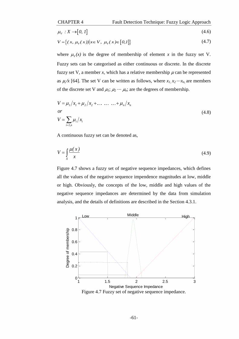
CHAPTER 4 Fault Detection Technique: Fuzzy Logic Approach
-61-
V : X 0, 1 (4.6)
V VV ( x, ( x )) x V , ( x ) 0,1 (4.7)
where V (x) is the degree of membership of element x in the fuzzy set V.
Fuzzy sets can be categorised as either continuous or discrete. In the discrete
fuzzy set V, a member x, which has a relative membership μ can be represented
as μ∕x [64]. The set V can be written as follows, where x1, x2 ⋯xn, are members
of the discrete set V and 1; 2 ⋯ n; are the degrees of membership.
1 1 2 2 n n
i i
i 1,n
V x x x
or
V x
(4.8)
A continuous fuzzy set can be denoted as,
X
( x )V
x
(4.9)
Figure 4.7 shows a fuzzy set of negative sequence impedances, which defines
all the values of the negative sequence impendence magnitudes at low, middle
or high. Obviously, the concepts of the low, middle and high values of the
negative sequence impedances are determined by the data from simulation
analysis, and the details of definitions are described in the Section 4.3.1.
Figure 4.7 Fuzzy set of negative sequence impedance.
1 1.5 2 2.5 30
0.2
0.4
0.6
0.8
1
Negative Sequence Impedance
Degre
e o
f m
em
bers
hip
Low Middle High
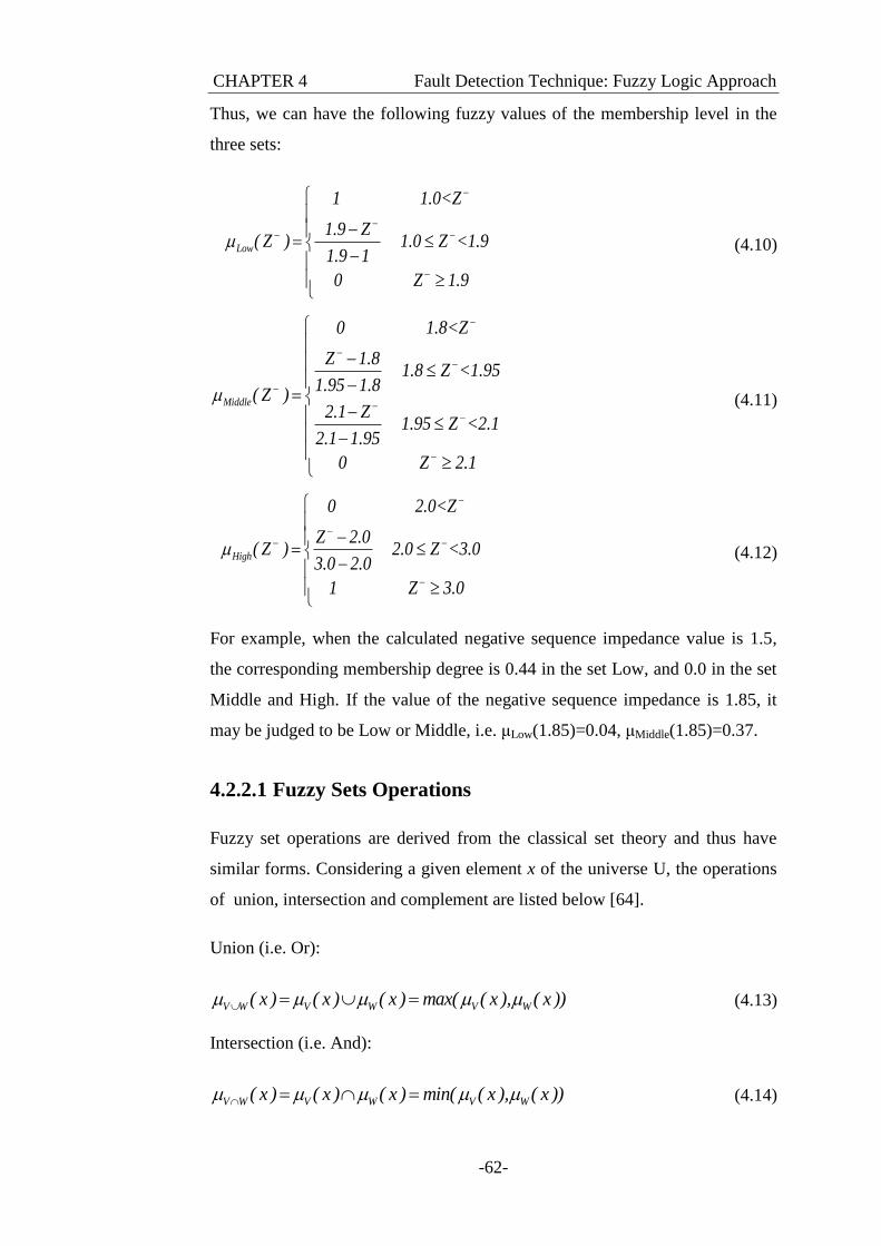
CHAPTER 4 Fault Detection Technique: Fuzzy Logic Approach
-62-
Thus, we can have the following fuzzy values of the membership level in the
three sets:
Low
1 1.0<Z
1.9 Z ( Z ) 1.0 Z <1.9
1.9 1
0 Z 1.9
(4.10)
Middle
0 1.8<Z
Z 1.8 1.8 Z <1.95
1.95 1.8( Z )
2.1 Z 1.95 Z <2.1
2.1 1.95
0 Z 2.1
(4.11)
High
0 2.0<Z
Z 2.0 ( Z ) 2.0 Z <3.0
3.0 2.0
1 Z 3.0
(4.12)
For example, when the calculated negative sequence impedance value is 1.5,
the corresponding membership degree is 0.44 in the set Low, and 0.0 in the set
Middle and High. If the value of the negative sequence impedance is 1.85, it
may be judged to be Low or Middle, i.e. μLow(1.85)=0.04, μMiddle(1.85)=0.37.
4.2.2.1 Fuzzy Sets Operations
Fuzzy set operations are derived from the classical set theory and thus have
similar forms. Considering a given element x of the universe U, the operations
of union, intersection and complement are listed below [64].
Union (i.e. Or):
V W V W V W( x ) ( x ) ( x ) max( ( x ), ( x )) (4.13)
Intersection (i.e. And):
V W V W V W( x ) ( x ) ( x ) min( ( x ), ( x )) (4.14)
CHAPTER 4 Fault Detection Technique: Fuzzy Logic Approach
-63-
Complement (i.e. Not):
V V( x ) 1 ( x ) (4.15)
Take the Low and Middle sets of Figure 4.7 for example,
Low 0.27 1.65 0.16 1.75 0.04 1.85 0 1.95 0 2.05
Middle 0 1.65 0 1.75 0.33 1.85 1 1.95 0.33 2.05
(4.16)
The union of the fuzzy sets Low and Middle
0.27 1.65 0.16 1.75 0.33 1.85 1 1.95 0.33 2.05 (4.17)
The intersection of the fuzzy sets Low and Middle
0 1.65 0 1.75 0.04 1.85 0 1.95 0 2.05 (4.18)
The complement of the fuzzy set Low
0.73 1.65 0.84 1.75 0.67 1.85 0 1.95 0.67 2.05 (4.19)
4.2.3 Fuzzy (Rule-Based) System
Generally, a fuzzy rule has the form as in (4.20), where V and W are two
classical sets that are defined on two universe sets X and Y, respectively.
If x is V, then y is W (4.20)
The if-part of the sentence is called the premise of the rule; the then-part of the
sentence is called the conclusion of the rule. It typically expresses an inference
such that if there is a fact, then another fact can inferred or derived [64, 67]. It
should be pointed out that, both the premise and conclusion of a rule may
contain multiple parts [68].
Figure 4.8 shows a simple Mamdani model of two-rule system. It has two crisp
values inputs x and y and a single output z*. Equation (4.21) gives the If-Then
rules used in the fuzzy system,
1 1 1
2 2 2
If x is A and y is B , then z is C
If x is A and y is B , then z is C (4.21)
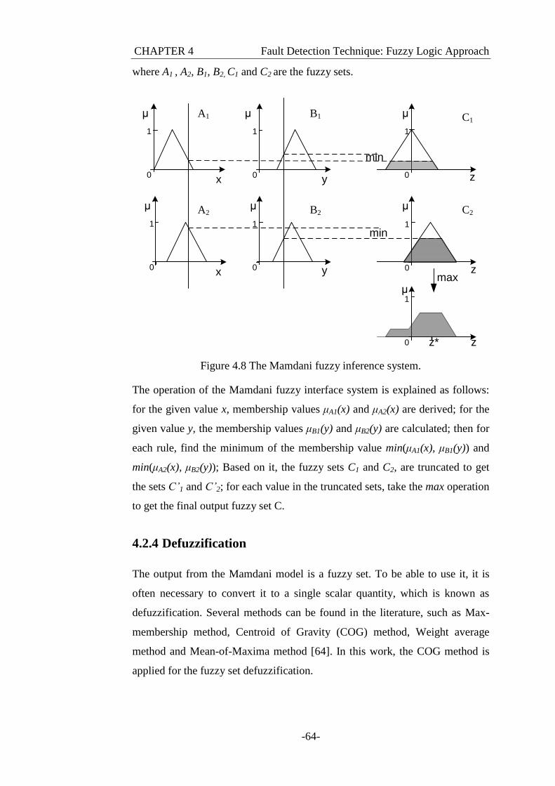
CHAPTER 4 Fault Detection Technique: Fuzzy Logic Approach
-64-
where A1 , A2, B1, B2, C1 and C2 are the fuzzy sets.
μ
μ μ
x y
A1 B1
z
μ
z
C2
min
μ
x
A2
y
B2
μ C1
min
μ
z
max
z*
0
1
0
1
0
1
0
1
0
1
0
1
0
1
Figure 4.8 The Mamdani fuzzy inference system.
The operation of the Mamdani fuzzy interface system is explained as follows:
for the given value x, membership values μA1(x) and μA2(x) are derived; for the
given value y, the membership values μB1(y) and μB2(y) are calculated; then for
each rule, find the minimum of the membership value min(μA1(x), μB1(y)) and
min(μA2(x), μB2(y)); Based on it, the fuzzy sets C1 and C2, are truncated to get
the sets C’1 and C’2; for each value in the truncated sets, take the max operation
to get the final output fuzzy set C.
4.2.4 Defuzzification
The output from the Mamdani model is a fuzzy set. To be able to use it, it is
often necessary to convert it to a single scalar quantity, which is known as
defuzzification. Several methods can be found in the literature, such as Max-
membership method, Centroid of Gravity (COG) method, Weight average
method and Mean-of-Maxima method [64]. In this work, the COG method is
applied for the fuzzy set defuzzification.
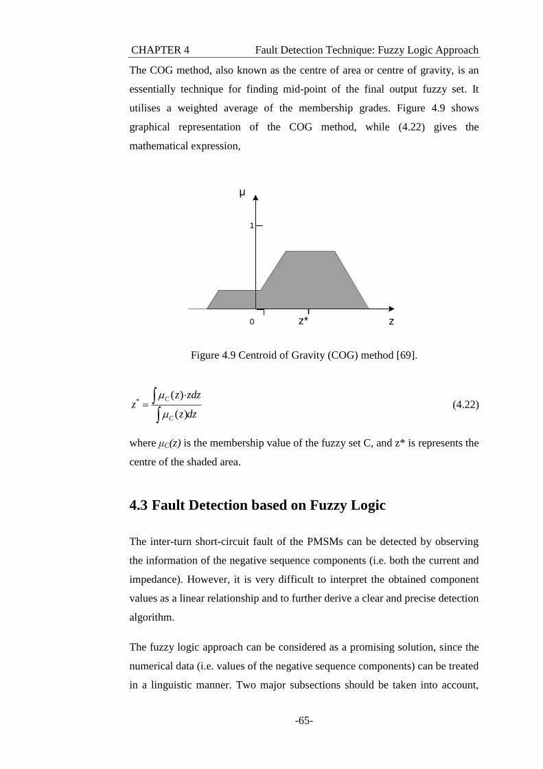
CHAPTER 4 Fault Detection Technique: Fuzzy Logic Approach
-65-
The COG method, also known as the centre of area or centre of gravity, is an
essentially technique for finding mid-point of the final output fuzzy set. It
utilises a weighted average of the membership grades. Figure 4.9 shows
graphical representation of the COG method, while (4.22) gives the
mathematical expression,
μ
1
z* z0
Figure 4.9 Centroid of Gravity (COG) method [69].
*( )
( )
C
C
z zdzz
z dz
(4.22)
where μC(z) is the membership value of the fuzzy set C, and z* is represents the
centre of the shaded area.
4.3 Fault Detection based on Fuzzy Logic
The inter-turn short-circuit fault of the PMSMs can be detected by observing
the information of the negative sequence components (i.e. both the current and
impedance). However, it is very difficult to interpret the obtained component
values as a linear relationship and to further derive a clear and precise detection
algorithm.
The fuzzy logic approach can be considered as a promising solution, since the
numerical data (i.e. values of the negative sequence components) can be treated
in a linguistic manner. Two major subsections should be taken into account,
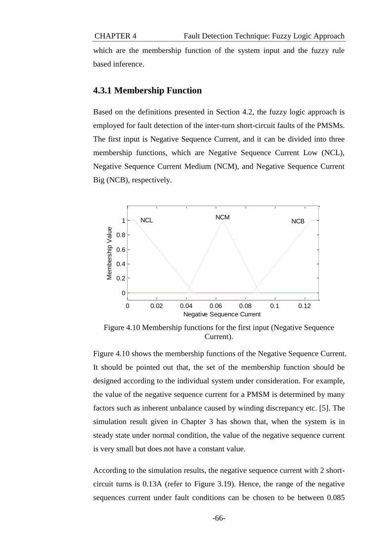
CHAPTER 4 Fault Detection Technique: Fuzzy Logic Approach
-66-
which are the membership function of the system input and the fuzzy rule
based inference.
4.3.1 Membership Function
Based on the definitions presented in Section 4.2, the fuzzy logic approach is
employed for fault detection of the inter-turn short-circuit faults of the PMSMs.
The first input is Negative Sequence Current, and it can be divided into three
membership functions, which are Negative Sequence Current Low (NCL),
Negative Sequence Current Medium (NCM), and Negative Sequence Current
Big (NCB), respectively.
Figure 4.10 Membership functions for the first input (Negative Sequence
Current).
Figure 4.10 shows the membership functions of the Negative Sequence Current.
It should be pointed out that, the set of the membership function should be
designed according to the individual system under consideration. For example,
the value of the negative sequence current for a PMSM is determined by many
factors such as inherent unbalance caused by winding discrepancy etc. [5]. The
simulation result given in Chapter 3 has shown that, when the system is in
steady state under normal condition, the value of the negative sequence current
is very small but does not have a constant value.
According to the simulation results, the negative sequence current with 2 short-
circuit turns is 0.13A (refer to Figure 3.19). Hence, the range of the negative
sequences current under fault conditions can be chosen to be between 0.085
0 0.02 0.04 0.06 0.08 0.1 0.12
0
0.2
0.4
0.6
0.8
1
Negative Sequence Current
Mem
bers
hip
Valu
e
NCL NCMNCB
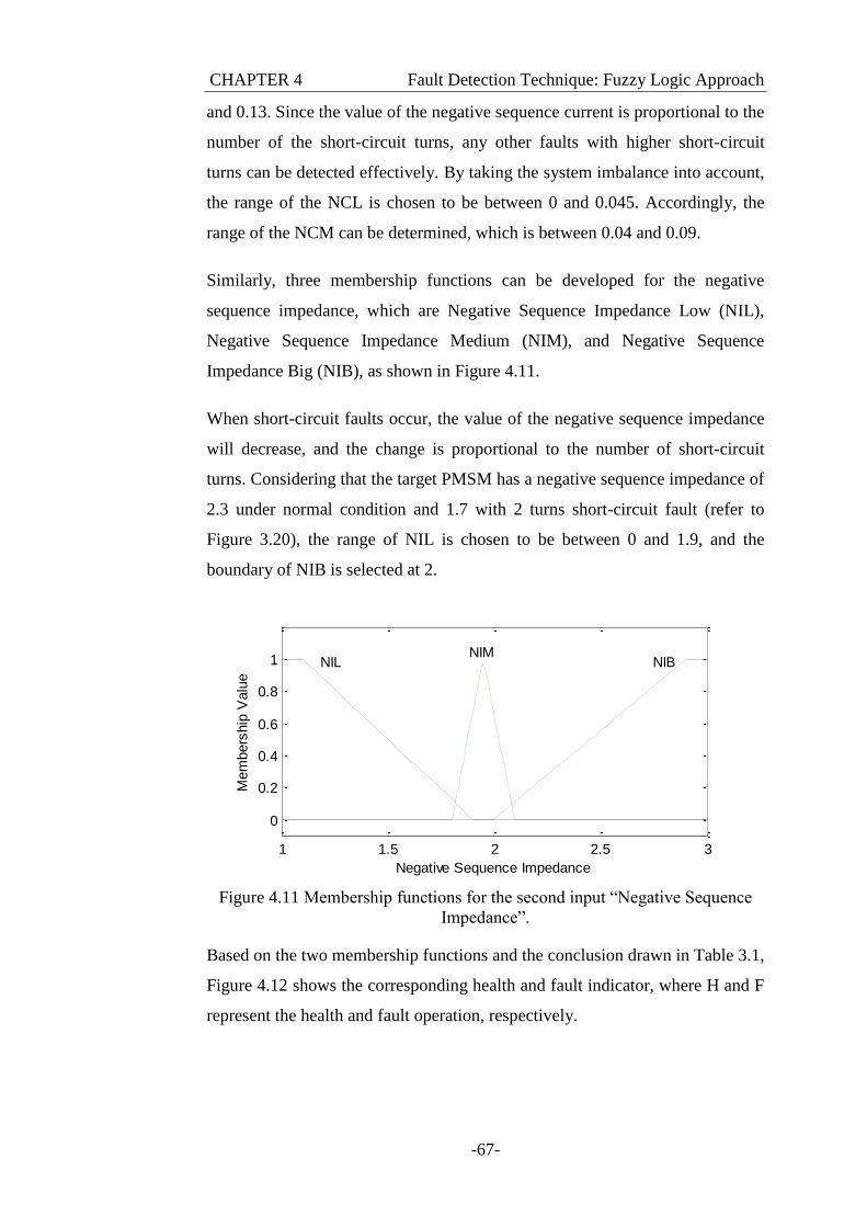
CHAPTER 4 Fault Detection Technique: Fuzzy Logic Approach
-67-
and 0.13. Since the value of the negative sequence current is proportional to the
number of the short-circuit turns, any other faults with higher short-circuit
turns can be detected effectively. By taking the system imbalance into account,
the range of the NCL is chosen to be between 0 and 0.045. Accordingly, the
range of the NCM can be determined, which is between 0.04 and 0.09.
Similarly, three membership functions can be developed for the negative
sequence impedance, which are Negative Sequence Impedance Low (NIL),
Negative Sequence Impedance Medium (NIM), and Negative Sequence
Impedance Big (NIB), as shown in Figure 4.11.
When short-circuit faults occur, the value of the negative sequence impedance
will decrease, and the change is proportional to the number of short-circuit
turns. Considering that the target PMSM has a negative sequence impedance of
2.3 under normal condition and 1.7 with 2 turns short-circuit fault (refer to
Figure 3.20), the range of NIL is chosen to be between 0 and 1.9, and the
boundary of NIB is selected at 2.
Figure 4.11 Membership functions for the second input “Negative Sequence
Impedance”.
Based on the two membership functions and the conclusion drawn in Table 3.1,
Figure 4.12 shows the corresponding health and fault indicator, where H and F
represent the health and fault operation, respectively.
1 1.5 2 2.5 3
0
0.2
0.4
0.6
0.8
1
Negative Sequence Impedance
Mem
bers
hip
Valu
e
NILNIM
NIB
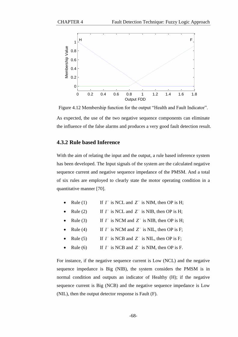
CHAPTER 4 Fault Detection Technique: Fuzzy Logic Approach
-68-
Figure 4.12 Membership function for the output “Health and Fault Indicator”.
As expected, the use of the two negative sequence components can eliminate
the influence of the false alarms and produces a very good fault detection result.
4.3.2 Rule based Inference
With the aim of relating the input and the output, a rule based inference system
has been developed. The Input signals of the system are the calculated negative
sequence current and negative sequence impedance of the PMSM. And a total
of six rules are employed to clearly state the motor operating condition in a
quantitative manner [70].
Rule (1) If I is NCL and Z is NIM, then OP is H;
Rule (2) If I is NCL and Z is NIB, then OP is H;
Rule (3) If I is NCM and Z is NIB, then OP is H;
Rule (4) If I is NCM and Z is NIL, then OP is F;
Rule (5) If I is NCB and Z is NIL, then OP is F;
Rule (6) If I is NCB and Z is NIM, then OP is F.
For instance, if the negative sequence current is Low (NCL) and the negative
sequence impedance is Big (NIB), the system considers the PMSM is in
normal condition and outputs an indicator of Healthy (H); if the negative
sequence current is Big (NCB) and the negative sequence impedance is Low
(NIL), then the output detector response is Fault (F).
0 0.2 0.4 0.6 0.8 1 1.2 1.4 1.6 1.8
0
0.2
0.4
0.6
0.8
1
Output FDD
Mem
bers
hip
Valu
e
H F
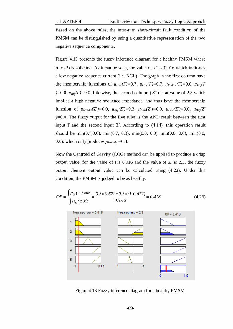
CHAPTER 4 Fault Detection Technique: Fuzzy Logic Approach
-69-
Based on the above rules, the inter-turn short-circuit fault condition of the
PMSM can be distinguished by using a quantitative representation of the two
negative sequence components.
Figure 4.13 presents the fuzzy inference diagram for a healthy PMSM where
rule (2) is solicited. As it can be seen, the value of I is 0.016 which indicates
a low negative sequence current (i.e. NCL). The graph in the first column have
the membership functions of μLow(I-)=0.7, μLow(I
-)=0.7, μMiddle(I
-)=0.0, μBig(I
-
)=0.0, μBig(I-)=0.0. Likewise, the second column ( Z ) is at value of 2.3 which
implies a high negative sequence impedance, and thus have the membership
function of μMiddle(Z-)=0.0, μBig(Z
-)=0.3, μLow(Z
-)=0.0, μLow(Z
-)=0.0, μBig(Z
-
)=0.0. The fuzzy output for the five rules is the AND result between the first
input I-
and the second input Z-. According to (4.14), this operation result
should be min(0.7,0.0), min(0.7, 0.3), min(0.0, 0.0), min(0.0, 0.0), min(0.0,
0.0), which only produces μHealthy=0.3.
Now the Centroid of Gravity (COG) method can be applied to produce a crisp
output value, for the value of I-is 0.016 and the value of Z
- is 2.3, the fuzzy
output element output value can be calculated using (4.22), Under this
condition, the PMSM is judged to be as healthy.
H
H
( z ) zdz 0.3 0.672+0.3 (1-0.672)OP 0.418
0.3 2( z )dz
(4.23)
Figure 4.13 Fuzzy inference diagram for a healthy PMSM.
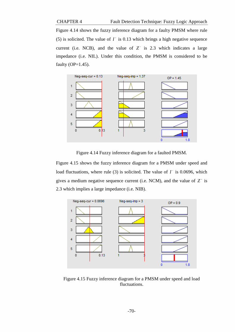
CHAPTER 4 Fault Detection Technique: Fuzzy Logic Approach
-70-
Figure 4.14 shows the fuzzy inference diagram for a faulty PMSM where rule
(5) is solicited. The value of I is 0.13 which brings a high negative sequence
current (i.e. NCB), and the value of Z is 2.3 which indicates a large
impedance (i.e. NIL). Under this condition, the PMSM is considered to be
faulty (OP=1.45).
Figure 4.14 Fuzzy inference diagram for a faulted PMSM.
Figure 4.15 shows the fuzzy inference diagram for a PMSM under speed and
load fluctuations, where rule (3) is solicited. The value of I is 0.0696, which
gives a medium negative sequence current (i.e. NCM), and the value of Z is
2.3 which implies a large impedance (i.e. NIB).
Figure 4.15 Fuzzy inference diagram for a PMSM under speed and load
fluctuations.
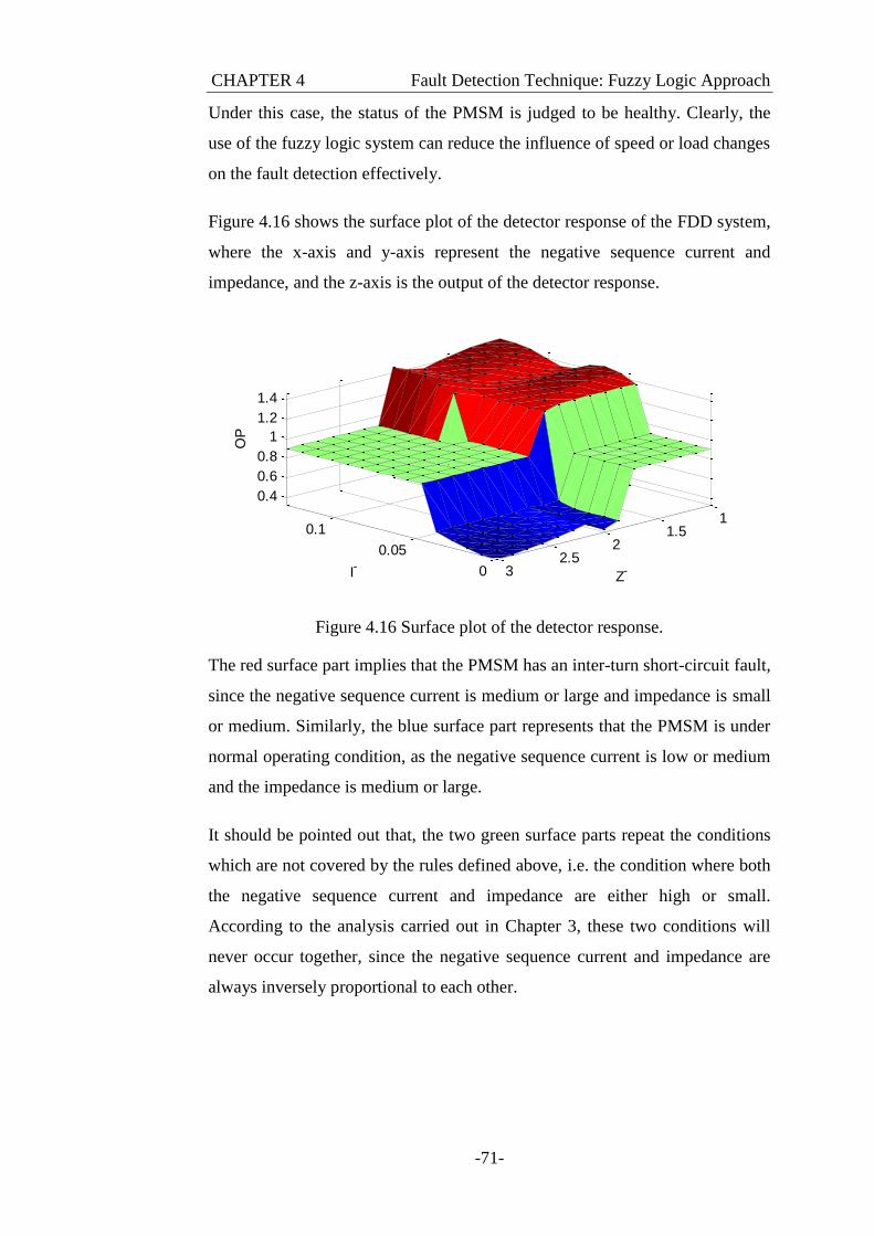
CHAPTER 4 Fault Detection Technique: Fuzzy Logic Approach
-71-
Under this case, the status of the PMSM is judged to be healthy. Clearly, the
use of the fuzzy logic system can reduce the influence of speed or load changes
on the fault detection effectively.
Figure 4.16 shows the surface plot of the detector response of the FDD system,
where the x-axis and y-axis represent the negative sequence current and
impedance, and the z-axis is the output of the detector response.
Figure 4.16 Surface plot of the detector response.
The red surface part implies that the PMSM has an inter-turn short-circuit fault,
since the negative sequence current is medium or large and impedance is small
or medium. Similarly, the blue surface part represents that the PMSM is under
normal operating condition, as the negative sequence current is low or medium
and the impedance is medium or large.
It should be pointed out that, the two green surface parts repeat the conditions
which are not covered by the rules defined above, i.e. the condition where both
the negative sequence current and impedance are either high or small.
According to the analysis carried out in Chapter 3, these two conditions will
never occur together, since the negative sequence current and impedance are
always inversely proportional to each other.
0
0.05
0.11
1.52
2.53
0.4
0.6
0.8
1
1.2
1.4
Z-I-
OP
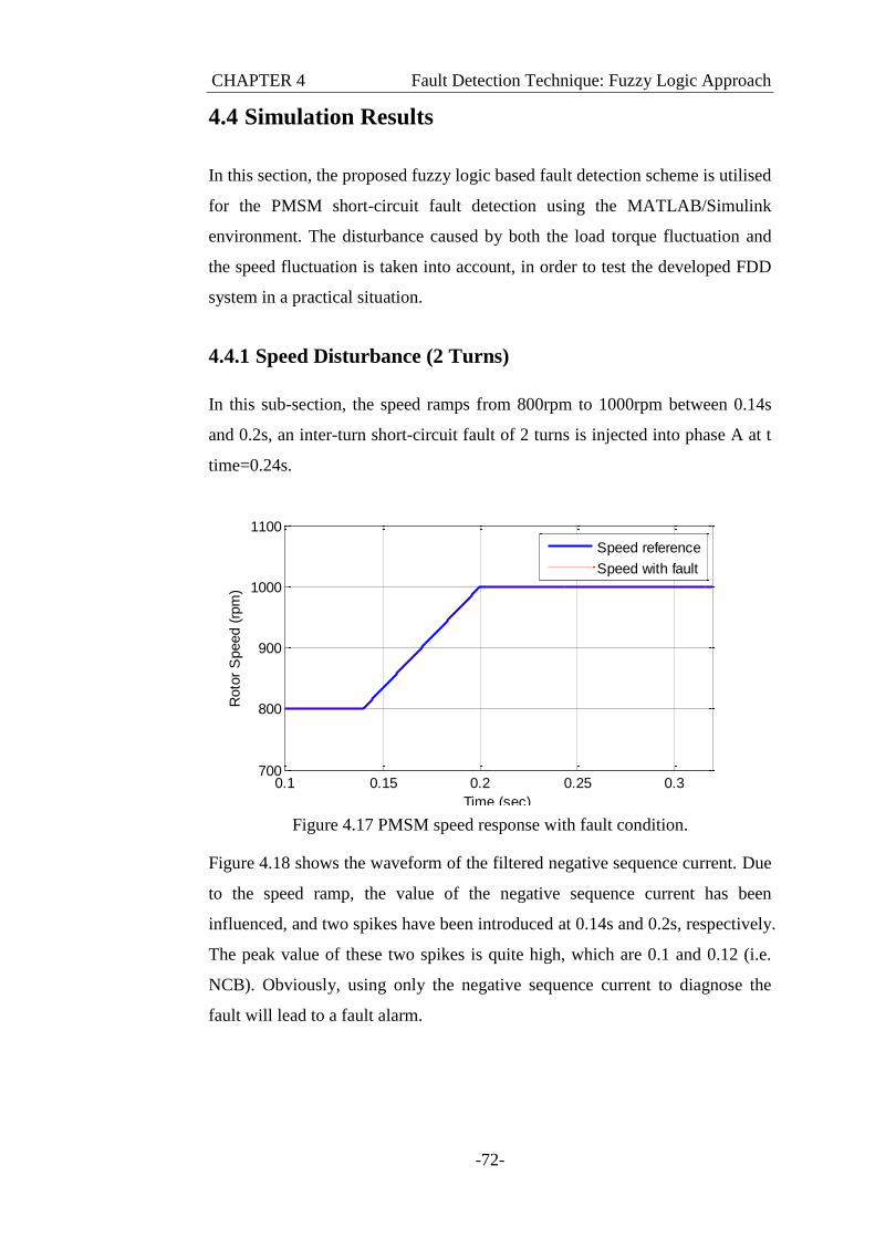
CHAPTER 4 Fault Detection Technique: Fuzzy Logic Approach
-72-
4.4 Simulation Results
In this section, the proposed fuzzy logic based fault detection scheme is utilised
for the PMSM short-circuit fault detection using the MATLAB/Simulink
environment. The disturbance caused by both the load torque fluctuation and
the speed fluctuation is taken into account, in order to test the developed FDD
system in a practical situation.
4.4.1 Speed Disturbance (2 Turns)
In this sub-section, the speed ramps from 800rpm to 1000rpm between 0.14s
and 0.2s, an inter-turn short-circuit fault of 2 turns is injected into phase A at t
time=0.24s.
Figure 4.17 PMSM speed response with fault condition.
Figure 4.18 shows the waveform of the filtered negative sequence current. Due
to the speed ramp, the value of the negative sequence current has been
influenced, and two spikes have been introduced at 0.14s and 0.2s, respectively.
The peak value of these two spikes is quite high, which are 0.1 and 0.12 (i.e.
NCB). Obviously, using only the negative sequence current to diagnose the
fault will lead to a fault alarm.
0.1 0.15 0.2 0.25 0.3700
800
900
1000
1100
Time (sec)
Roto
r S
peed (
rpm
)
Speed reference
Speed with fault
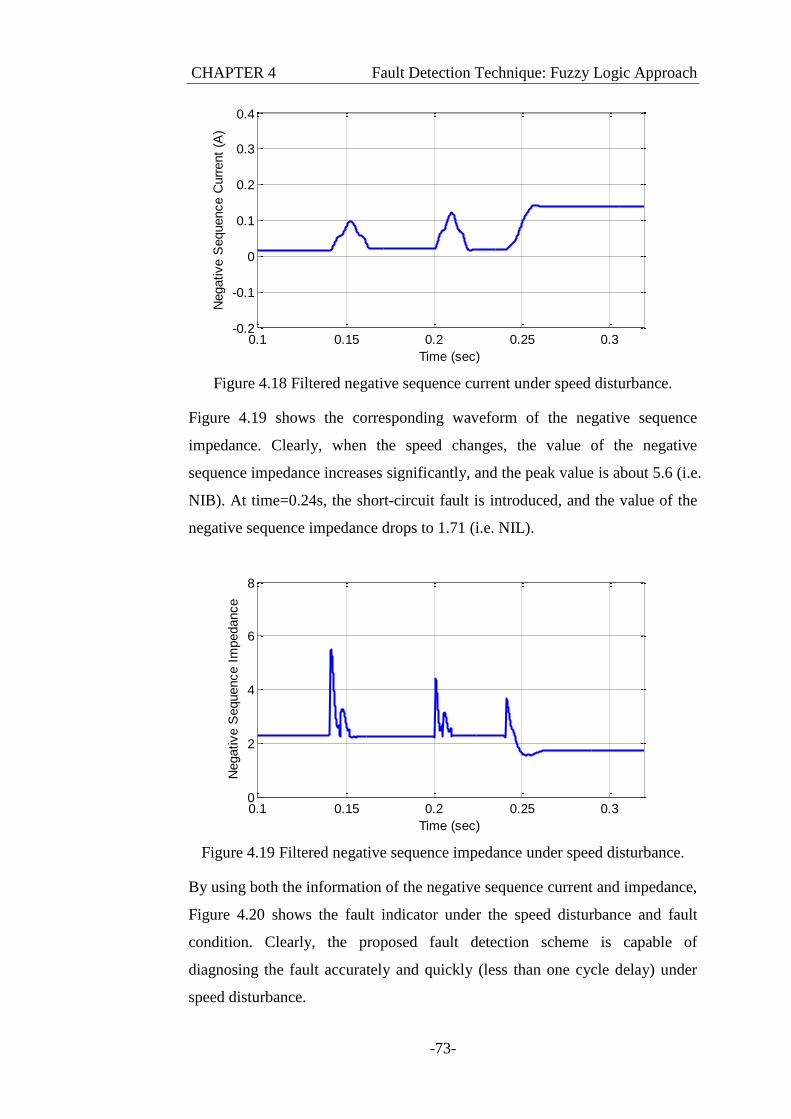
CHAPTER 4 Fault Detection Technique: Fuzzy Logic Approach
-73-
Figure 4.18 Filtered negative sequence current under speed disturbance.
Figure 4.19 shows the corresponding waveform of the negative sequence
impedance. Clearly, when the speed changes, the value of the negative
sequence impedance increases significantly, and the peak value is about 5.6 (i.e.
NIB). At time=0.24s, the short-circuit fault is introduced, and the value of the
negative sequence impedance drops to 1.71 (i.e. NIL).
Figure 4.19 Filtered negative sequence impedance under speed disturbance.
By using both the information of the negative sequence current and impedance,
Figure 4.20 shows the fault indicator under the speed disturbance and fault
condition. Clearly, the proposed fault detection scheme is capable of
diagnosing the fault accurately and quickly (less than one cycle delay) under
speed disturbance.
0.1 0.15 0.2 0.25 0.3-0.2
-0.1
0
0.1
0.2
0.3
0.4
Time (sec)
Negative S
equence C
urr
ent
(A)
0.1 0.15 0.2 0.25 0.30
2
4
6
8
Time (sec)
Negative S
equence I
mpedance
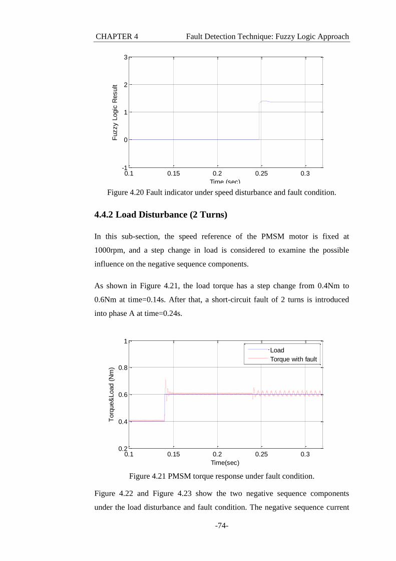
CHAPTER 4 Fault Detection Technique: Fuzzy Logic Approach
-74-
Figure 4.20 Fault indicator under speed disturbance and fault condition.
4.4.2 Load Disturbance (2 Turns)
In this sub-section, the speed reference of the PMSM motor is fixed at
1000rpm, and a step change in load is considered to examine the possible
influence on the negative sequence components.
As shown in Figure 4.21, the load torque has a step change from 0.4Nm to
0.6Nm at time=0.14s. After that, a short-circuit fault of 2 turns is introduced
into phase A at time=0.24s.
Figure 4.21 PMSM torque response under fault condition.
Figure 4.22 and Figure 4.23 show the two negative sequence components
under the load disturbance and fault condition. The negative sequence current
0.1 0.15 0.2 0.25 0.3-1
0
1
2
3
Time (sec)
Fuzzy L
ogic
Result
0.1 0.15 0.2 0.25 0.30.2
0.4
0.6
0.8
1
Time(sec)
Torq
ue&
Load (
Nm
)
Load
Torque with fault
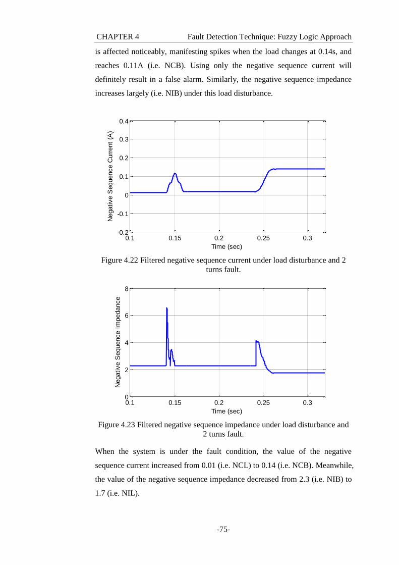
CHAPTER 4 Fault Detection Technique: Fuzzy Logic Approach
-75-
is affected noticeably, manifesting spikes when the load changes at 0.14s, and
reaches 0.11A (i.e. NCB). Using only the negative sequence current will
definitely result in a false alarm. Similarly, the negative sequence impedance
increases largely (i.e. NIB) under this load disturbance.
Figure 4.22 Filtered negative sequence current under load disturbance and 2
turns fault.
Figure 4.23 Filtered negative sequence impedance under load disturbance and
2 turns fault.
When the system is under the fault condition, the value of the negative
sequence current increased from 0.01 (i.e. NCL) to 0.14 (i.e. NCB). Meanwhile,
the value of the negative sequence impedance decreased from 2.3 (i.e. NIB) to
1.7 (i.e. NIL).
0.1 0.15 0.2 0.25 0.3-0.2
-0.1
0
0.1
0.2
0.3
0.4
Time (sec)
Negative S
equence C
urr
ent
(A)
0.1 0.15 0.2 0.25 0.30
2
4
6
8
Time (sec)
Negative S
equence I
mpedance
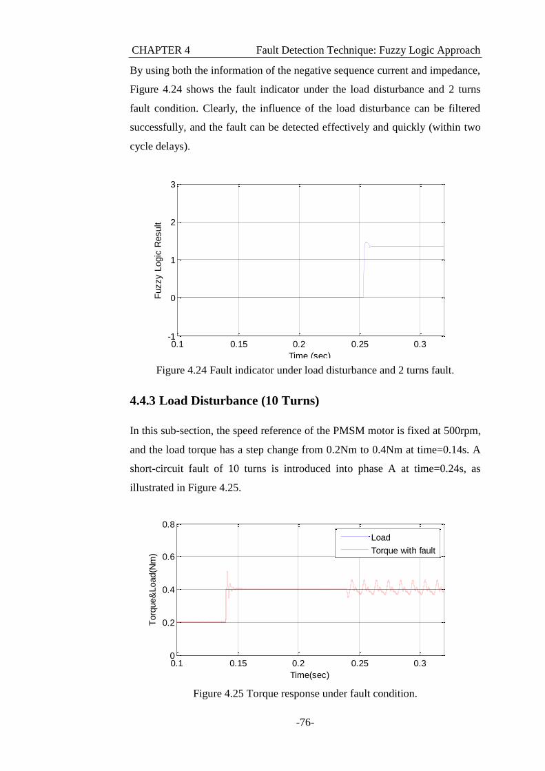
CHAPTER 4 Fault Detection Technique: Fuzzy Logic Approach
-76-
By using both the information of the negative sequence current and impedance,
Figure 4.24 shows the fault indicator under the load disturbance and 2 turns
fault condition. Clearly, the influence of the load disturbance can be filtered
successfully, and the fault can be detected effectively and quickly (within two
cycle delays).
Figure 4.24 Fault indicator under load disturbance and 2 turns fault.
4.4.3 Load Disturbance (10 Turns)
In this sub-section, the speed reference of the PMSM motor is fixed at 500rpm,
and the load torque has a step change from 0.2Nm to 0.4Nm at time=0.14s. A
short-circuit fault of 10 turns is introduced into phase A at time=0.24s, as
illustrated in Figure 4.25.
Figure 4.25 Torque response under fault condition.
0.1 0.15 0.2 0.25 0.3-1
0
1
2
3
Time (sec)
Fuzzy L
ogic
Result
0.1 0.15 0.2 0.25 0.30
0.2
0.4
0.6
0.8
Time(sec)
Torq
ue&
Load(N
m)
Load
Torque with fault
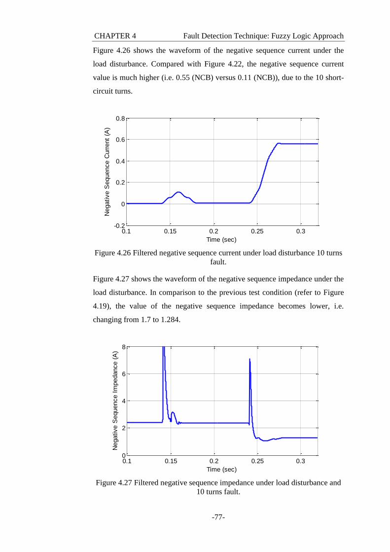
CHAPTER 4 Fault Detection Technique: Fuzzy Logic Approach
-77-
Figure 4.26 shows the waveform of the negative sequence current under the
load disturbance. Compared with Figure 4.22, the negative sequence current
value is much higher (i.e. 0.55 (NCB) versus 0.11 (NCB)), due to the 10 short-
circuit turns.
Figure 4.26 Filtered negative sequence current under load disturbance 10 turns
fault.
Figure 4.27 shows the waveform of the negative sequence impedance under the
load disturbance. In comparison to the previous test condition (refer to Figure
4.19), the value of the negative sequence impedance becomes lower, i.e.
changing from 1.7 to 1.284.
Figure 4.27 Filtered negative sequence impedance under load disturbance and
10 turns fault.
0.1 0.15 0.2 0.25 0.3-0.2
0
0.2
0.4
0.6
0.8
Time (sec)
Negative S
equence C
urr
ent
(A)
0.1 0.15 0.2 0.25 0.30
2
4
6
8
Time (sec)
Negative S
equence I
mpedance (
A)
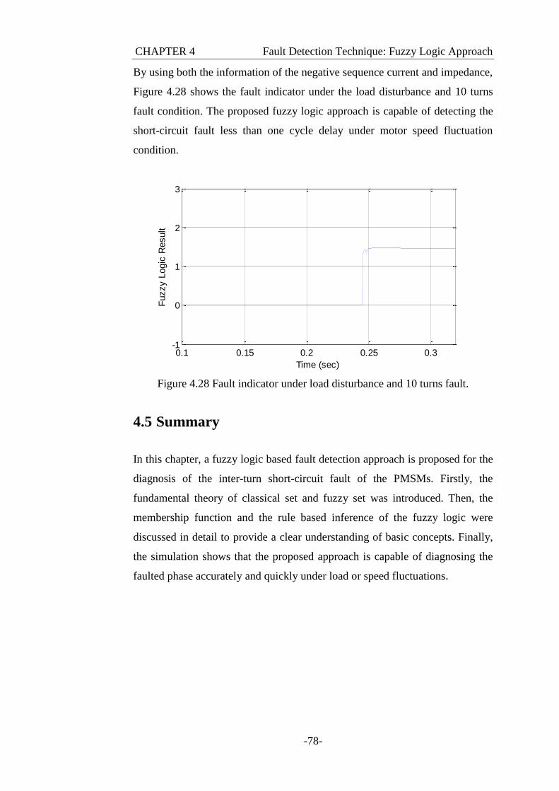
CHAPTER 4 Fault Detection Technique: Fuzzy Logic Approach
-78-
By using both the information of the negative sequence current and impedance,
Figure 4.28 shows the fault indicator under the load disturbance and 10 turns
fault condition. The proposed fuzzy logic approach is capable of detecting the
short-circuit fault less than one cycle delay under motor speed fluctuation
condition.
Figure 4.28 Fault indicator under load disturbance and 10 turns fault.
4.5 Summary
In this chapter, a fuzzy logic based fault detection approach is proposed for the
diagnosis of the inter-turn short-circuit fault of the PMSMs. Firstly, the
fundamental theory of classical set and fuzzy set was introduced. Then, the
membership function and the rule based inference of the fuzzy logic were
discussed in detail to provide a clear understanding of basic concepts. Finally,
the simulation shows that the proposed approach is capable of diagnosing the
faulted phase accurately and quickly under load or speed fluctuations.
0.1 0.15 0.2 0.25 0.3-1
0
1
2
3
Time (sec)
Fuzzy L
ogic
Result
CHAPTER 5 Conclusions and Future Work
-79-
CHAPTER 5
CONCLUSIONS AND
FUTURE WORK
5.1 Conclusions
In the last two decades, the permanent magnet synchronous machine has
attracted more and more interests and been applied widely in modern industries
and special applications, such as hybrid automobile, aerospace drives and
military power drives. Owing to the high energy product of rare-earth
permanent magnet, the PMSMs hold excellent torque density, wide constant
power speed range and high conversion efficiency in comparison of traditional
machines. However, the use of the permanent magnet for the creation of the
magnetic field brings a significant drawback for the machine, which is the
weak fault tolerance capability. Taking an inter-turn short-circuit fault as an
example, a few short-circuit turns lead to huge increase in the faulting winding
current, and thus to excessive heat generation. This may further propagate and
eventually cause a catastrophic failure.
CHAPTER 5 Conclusions and Future Work
-80-
Based on the above reason, fault detection of the PMSMs has become crucially
important and necessary, especially for applications demanding high security
and reliability (e.g. aerospace and automotive sectors). This forms the basic
motivation of this research work.
In this thesis, the modelling of PMSM with an inter-turn short-circuit faults
have been presented first. Based on the classical three-phase circuit coordinates,
the dynamic description of the PMSM under the ABC frame has been reviewed
and transformed into the DQ frame. The developed PMSM model can
represent the motor operation under the normal and short-circuit fault
conditions. The simulation results have shown a good correlation to the
theoretical analysis.
Following this, a winding inter-turn short-circuit fault detection technique for
the PMSM has been addressed by applying sequence component theory. Two
different ways for the derivation of the sequence component have been
demonstrated, and a three-phase sequence analyser is used to obtain the
negative sequence components for fault detection purpose. Although either the
negative sequence current or impedance can reflect the occurrence of a fault,
the influence of the motor speed or load fluctuation introduces disturbances
and, thus, false alarms, which makes the fault detection system unreliable.
In order to overcome this problem, a fuzzy logic approach has been considered
to process both the negative sequence current and impedance information, in
order to eliminate the disturbance of the load or speed fluctuation while the
true short-circuit fault can be diagnosed effectively and quickly. Based on a
number of different measured data from the simulation result, the fuzzy logic
system has been adjusted and tested. The simulation results have shown that
the proposed fault detection approach is capable of diagnosing the faulting
phase accurately and quickly under both load and speed fluctuations.
CHAPTER 5 Conclusions and Future Work
-81-
5.2 Future Work
Although the feasibility of the developed fault detection and diagnosis system
has been validated successfully, there are still some aspects that need to
improve and study further for practical applications.
Although the most common fault of the PMSMs, i.e. inter-turn short-circuit
type fault, has been studied and modelled in this thesis, the work on the PMSM
fault modelling could be further improved. For the considered fault model,
several assumptions were made for simplicity, such as sinusoidal distribution
of magneto motive force and the flux, and non-saturated magnetic field etc.
These assumptions may introduce model errors, and compromise the fidelity of
the model. Advanced modelling techniques could be employed to improve
accuracy.
Second, only the stator winding turn-to-turn short-circuit fault has been
considered. In practice, the PMSM may suffer from different faults, such as
inverter faults, air gap eccentricity, partial demagnetisation, etc. For a
comprehensive FDD system, different type of faults should be detected and
identified. The influence of other faults on the developed technique should also
be assessed.
Likewise, the effects of harmonics in the determination of the fault indicator
should also be studied. And finally, the proposed system should be tested in a
prototype drive system with controllable fault injections.
Appendix
-82-
Appendix A
SIMULINK MODELS
A.1 Simulink Models
In this Appendix, the detailed structure of the MatLab Simulink models
developed for the FDD of the PMSM is presented as follows.
Figure A.1 Simulink model of vector controlled PMSM.
Vd
Vq
the
Vabc
dq2abc
we
iq
Torque
we
id
0
I I_q_ref
Speed Controller
Speed Vabc Pulses
PWM
TL we
the
wm
id
iq
Va
Vb
Vc
Machine module
g
v a
v b
v c
Inverter
-K-
id_er
iq_er
v d_ref
v q_ref
Current Controller
Appendix
-83-
Figure A.2 Subsystem of the PMSM.
Figure A.3 Subsystem of the electrical model.
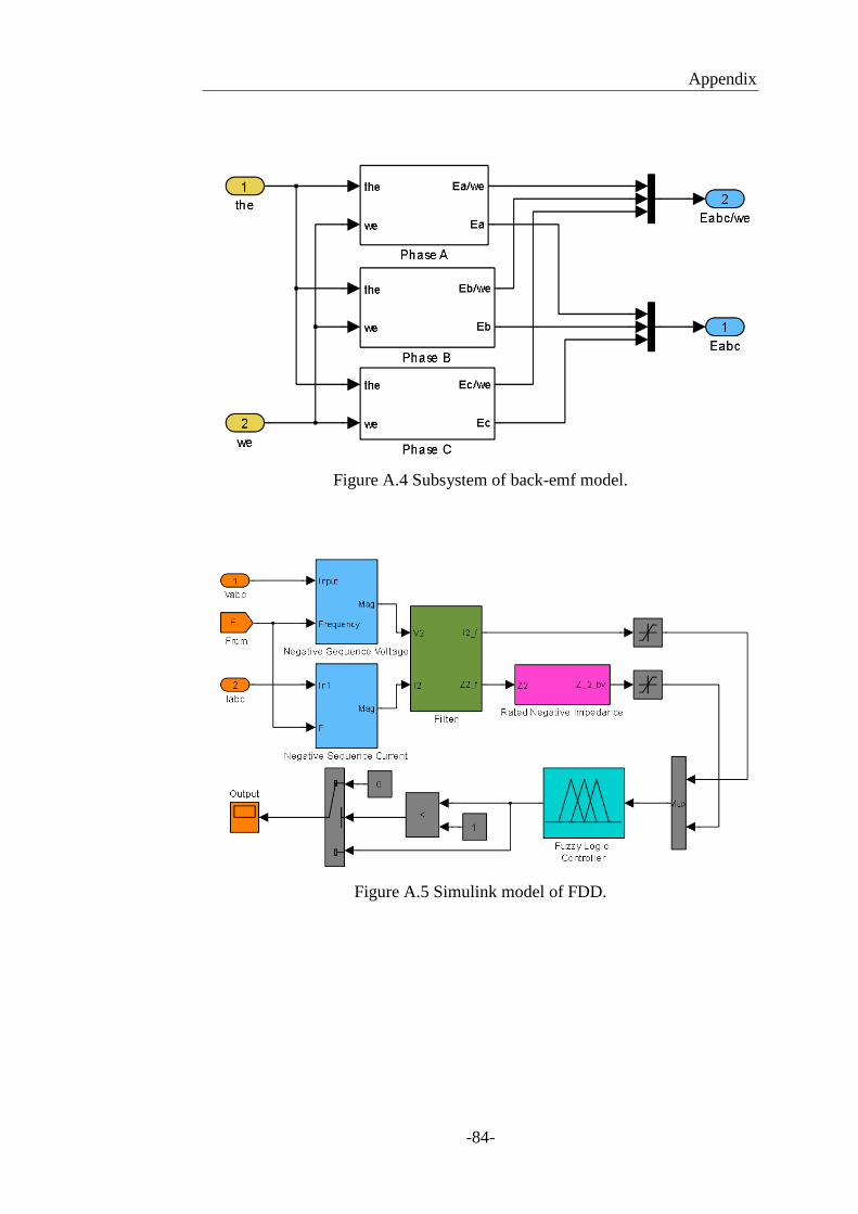
Appendix
-84-
Figure A.4 Subsystem of back-emf model.
Figure A.5 Simulink model of FDD.
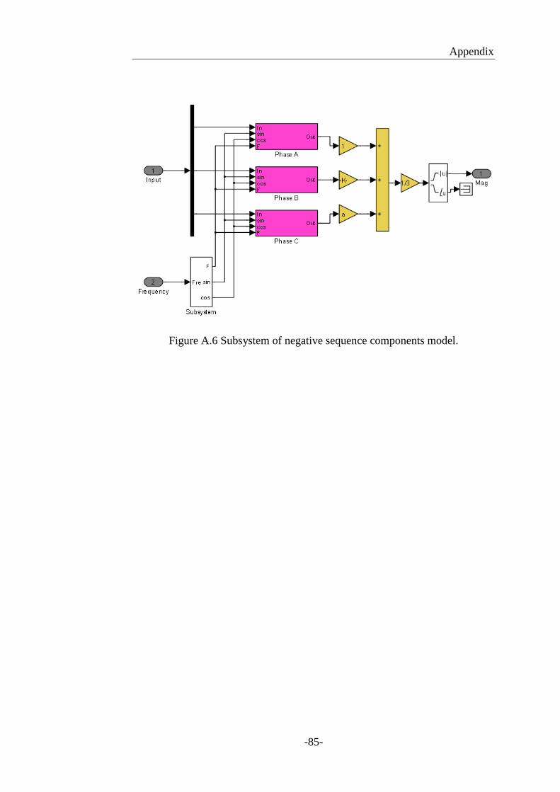
Appendix
-85-
Figure A.6 Subsystem of negative sequence components model.
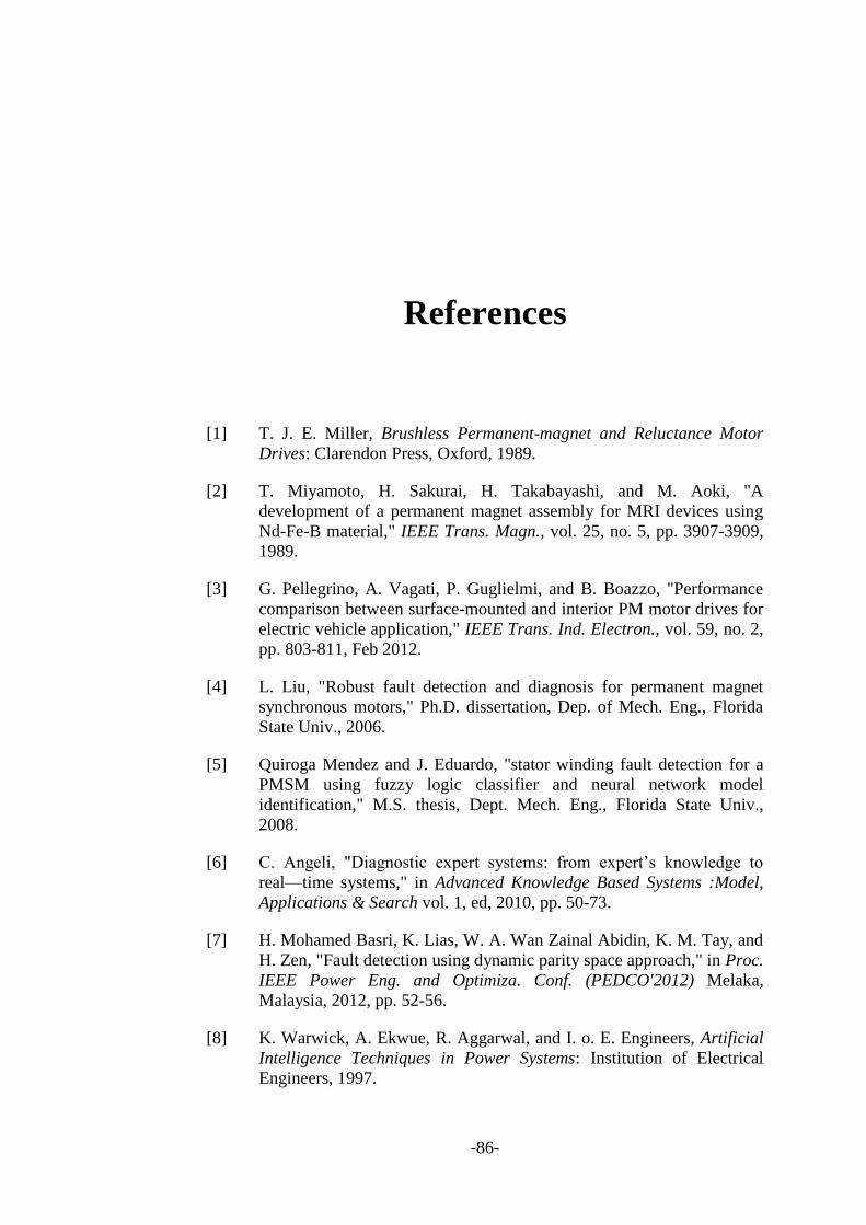
-86-
References
[1] T. J. E. Miller, Brushless Permanent-magnet and Reluctance Motor
Drives: Clarendon Press, Oxford, 1989.
[2] T. Miyamoto, H. Sakurai, H. Takabayashi, and M. Aoki, "A
development of a permanent magnet assembly for MRI devices using
Nd-Fe-B material," IEEE Trans. Magn., vol. 25, no. 5, pp. 3907-3909,
1989.
[3] G. Pellegrino, A. Vagati, P. Guglielmi, and B. Boazzo, "Performance
comparison between surface-mounted and interior PM motor drives for
electric vehicle application," IEEE Trans. Ind. Electron., vol. 59, no. 2,
pp. 803-811, Feb 2012.
[4] L. Liu, "Robust fault detection and diagnosis for permanent magnet
synchronous motors," Ph.D. dissertation, Dep. of Mech. Eng., Florida
State Univ., 2006.
[5] Quiroga Mendez and J. Eduardo, "stator winding fault detection for a
PMSM using fuzzy logic classifier and neural network model
identification," M.S. thesis, Dept. Mech. Eng., Florida State Univ.,
2008.
[6] C. Angeli, "Diagnostic expert systems: from expert’s knowledge to
real—time systems," in Advanced Knowledge Based Systems :Model,
Applications & Search vol. 1, ed, 2010, pp. 50-73.
[7] H. Mohamed Basri, K. Lias, W. A. Wan Zainal Abidin, K. M. Tay, and
H. Zen, "Fault detection using dynamic parity space approach," in Proc.
IEEE Power Eng. and Optimiza. Conf. (PEDCO'2012) Melaka,
Malaysia, 2012, pp. 52-56.
[8] K. Warwick, A. Ekwue, R. Aggarwal, and I. o. E. Engineers, Artificial
Intelligence Techniques in Power Systems: Institution of Electrical
Engineers, 1997.
-87-
[9] G. K. Singh and S. a. Ahmed Saleh Al Kazzaz, "Induction machine
drive condition monitoring and diagnostic research—a survey," Electric
Power Systems Research, vol. 64, pp. 145-158, 2003.
[10] J. Robinson, C. Whelan, and N. K. Haggerty, "Trends in advanced
motor protection and monitoring," IEEE Trans. Ind. Appl., vol. 40, pp.
853-860, 2004.
[11] S. Nandi and H. A. Toliyat, "Condition monitoring and fault diagnosis
of electrical machines-a review," in Proc. 34th. Annu. Conf. IEEE Ind.
Applicat. Conf. (IAS'99), Phoenix, AZ, 1999, pp. 197-204.
[12] "IEEE Recommended Practice for the Design of Reliable Industrial and
Commercial Power Systems - Redline," IEEE Std 493-2007 (Revision
of IEEE Std 493-1997) - Redline, pp. 1-426, 2007.
[13] O. Ojo, O. Osaloni, and P. Kshirsagar, "Models for the control and
simulation of synchronous type machine drives under various fault
conditions," in Proc. 37th. Annu. Conf. IEEE Ind. Appl. Conf. (IAS'02),
Pittsburgh, PA, 2002, pp. 1533-1540.
[14] A. A. Abdallah, V. Devanneaux, J. Faucher, B. Dagues, and A. Randria,
"Modelling of surface-mounted permanent magnet synchronous
machines with stator faults," in Proc. 30th. Annu. Conf. IEEE Ind.
Electon. Soc. (IECON'04), Busan, Korea, 2004, pp. 3031-3036.
[15] S. Nandi, H. A. Toliyat, and L. Xiaodong, "Condition monitoring and
fault diagnosis of electrical motors-a review," IEEE Trans. Energy
Convers., vol. 20, pp. 719-729, 2005.
[16] A. L. Nelson and C. Mo-Yuen, "Characterization of coil faults in an
axial flux variable reluctance PM motor," IEEE Trans. Energy Convers.,
vol. 17, pp. 340-348, 2002.
[17] A. Gandhi, T. Corrigan, and L. Parsa, "Recent advances in modeling
and online detection of stator interturn faults in electrical motors," IEEE
Trans. Ind. Electron., vol. 58, pp. 1564-1575, 2011.
[18] W. T. Thomson and M. Fenger, "Current signature analysis to detect
induction motor faults," in IEEE Ind. Appl. Mag. vol. 7, ed, 2001, pp.
26-34.
[19] W. Qing and S. Nandi, "Fast single-turn sensitive stator inter-turn fault
detection of induction mchines based on positive and negative sequence
third harmonic components of line currents," in Proc. 43th. Annu. Conf.
IEEE Ind. Appl. Conf. (IAS'08), Edmonton, Canada, 2008, pp. 1-8.
[20] J. Cusido, L. Romeral, J. A. Ortega, J. A. Rosero, and A. Garcia
Espinosa, "Fault detection in induction machines using power spectral
density in wavelet decomposition," IEEE Trans. Ind. Electron., vol. 55,
pp. 633-643, 2008.
-88-
[21] J. A. Rosero, L. Romeral, J. Cusido, A. Garcia, and J. A. Ortega, "On
the short-circuiting fault detection in a PMSM by means of stator
current transformations," in Proc. IEEE Power Electron. Specialists
Conf. (PESC'07), Orlando, Florida, 2007, pp. 1936-1941.
[22] P. S. Barendse, B. Herndler, M. A. Khan, and P. Pillay, "The
application of wavelets for the detection of inter-turn faults in induction
machines," in Proc. IEEE Int. Electric Machines and Drives Conf.
(IEMDC'09), Miami, United States, 2009, pp. 1401-1407.
[23] J. Rosero, L. Romeral, E. Rosero, and J. Urresty, "Fault detection in
dynamic conditions by means of discrete wavelet decomposition for
PMSM running under bearing damage," in Proc. 24th IEEE Appl.
Power Electron. Conf. and Exposition (APEC'09), Washington,USA,
2009, pp. 951-956.
[24] A. Bouzida, O. Touhami, R. Ibtiouen, A. Belouchrani, M. Fadel, and A.
Rezzoug, "Fault diagnosis in industrial induction machines through
discrete wavelet transform," IEEE Trans. Ind. Electron., vol. 58, pp.
4385-4395, 2011.
[25] H. Jun, Z. Jianzhong, C. Ming, and W. Zheng, "Fault diagnosis of
mechanical unbalance for permanent magnet synchronous motor drive
system under nonstationary condition," in Proc. IEEE Int. Energy
Convers. Congr. Expo. Conf. (ECCE' 2013), Denver, Colorado, 2013,
pp. 3556-3562.
[26] C. Siwei, Z. Pinjia, and T. G. Habetler, "An Impedance Identification
Approach to Sensitive Detection and Location of Stator Turn-to-Turn
Faults in a Closed-Loop Multiple-Motor Drive," IEEE Trans. Ind.
Electron., vol. 58, pp. 1545-1554, 2011.
[27] J. C. Urresty, J. R. Riba, H. Saavedra, and L. Romeral, "Detection of
inter-turns short circuits in permanent magnet synchronous motors
operating under transient conditions by means of the zero sequence
voltage," in Proc. 14th Euro. Conf. Power Electron. Appl. (EPE '11),
Birmingham, United Kingdom, 2011, pp. 1-9.
[28] L. A. Pereira, D. da Silva Gazzana, and L. F. A. Pereira, "Motor current
signature analysis and fuzzy logic applied to the diagnosis of short-
circuit faults in induction motors," in Proc. 31st IEEE Ann. Conf. Ind.
Electron. Soc. (IECON '05), Raleigh, NC, 2005, pp. 275-280.
[29] A. Siddique, G. S. Yadava, and B. Singh, "Applications of artificial
intelligence techniques for induction machine stator fault diagnostics:
review," in Proc. 4th IEEE Int. Symp. on Diagnostics for Electric
Mach., Power Electron. and Drives, (SDEMPED'03), Atlanta, Georgia,
USA, 2003, pp. 29-34.
[30] M. Bouzid, G. Champenois, N. M. Bellaaj, L. Signac, and K. Jelassi,
"An Effective Neural Approach for the Automatic Location of Stator
-89-
Interturn Faults in Induction Motor," IEEE Trans. Ind. Electron., vol.
55, pp. 4277-4289, 2008.
[31] B. C. Mecrow, A. G. Jack, J. A. Haylock, and J. Coles, "Fault tolerant
permanent magnet machine drives," in Proc. 17th IEEE Int. Conf. on
Elect. Mach. and Drives, 1995, pp. 433-437.
[32] J. A. Haylock, B. C. Mecrow, A. G. Jack, and D. J. Atkinson,
"Operation of fault tolerant machines with winding failures," IEEE
Trans. Energy Convers., vol. 14, pp. 1490-1495, 1999.
[33] Y. Lee, "A stator turn fault detection method and a fault-tolerant
operating strategy for interior PM synchronous motor drives in safety-
critical applications," Ph.D dissertation, Dep. of Elect. Comput. Eng.,
Georgia Institute of Technology, 2007.
[34] D. Min, A. Keyhani, and T. Sebastian, "Fault analysis of a PM
brushless DC Motor using finite element method," IEEE Trans. Energy
Convers., vol. 20, pp. 1-6, 2005.
[35] O. A. Mohammed, Z. Liu, S. Liu, and N. Y. Abed, "Internal Short
Circuit Fault Diagnosis for PM Machines Using FE-Based Phase
Variable Model and Wavelets Analysis," IEEE Trans. Magn., vol. 43,
pp. 1729-1732, 2007.
[36] T. R. Jawad Ahmed Farooq, Abdesslem Djerdir, Abdellatif Miraoui,
"Modelling and simulation of stator winding inter-turn faults in
permanent magnet synchronous motors," Int. J. Comput. Math. in Elect.
Electron. Eng. (COMPEL'08), vol. 27, pp. 887-896, 2008.
[37] D. Bao and W. Huo, "High precision BLDCM servo control with
nonlinear identification," in Informatics in Control, Automation and
Robotics. vol. 2, Y. Dehuai, Ed., ed: Springer, 2012, pp. 761-768.
[38] P. Pillay and R. Krishnan, "Modeling of permanent magnet motor
drives," IEEE Trans. Ind. Electron., vol. 35, pp. 537-541, 1988.
[39] R. H. Park, "Two-reaction theory of synchronous machines generalized
method of analysis-Part I," AIEE Tran., vol. 48, pp. 716-727, 1929.
[40] T. Boileau, B. Nahid-Mobarakeh, and F. Meibody-Tabar, "Back-EMF
based detection of stator winding inter-turn fault for PM synchronous
motor drives," in Proc. IEEE Conf. on Vehicle Power and Propulsion
(VPPC'07), Arlington, USA, 2007, pp. 95-100.
[41] L. Romeral, J. C. Urresty, J. R. Riba Ruiz, and A. Garcia Espinosa,
"Modeling of Surface-Mounted Permanent Magnet Synchronous
Motors With Stator Winding Interturn Faults," IEEE Trans. Ind.
Electron., vol. 58, pp. 1576-1585, 2011.
[42] B. Vaseghi, B. Nahid-Mobarakeh, N. Takorabet, and F. Meibody-Tabar,
"Experimentally validated fynamic fault model for PMSM with stator
-90-
winding inter-turn fault," in Proc. IEEE Ind. Appl. Soc. Ann. Meeting
(IAS '08), Edmonton, Canada 2008, pp. 1-5.
[43] M. E. H. Benbouzid, "A Review of Induction Motors Signature
Analysis as a Medium for Faults Detection," IEEE Trans. Ind. Electron.,
vol. 47, 2000.
[44] R. R. Schoen, T. G. Habetler, F. Kamran, and R. G. Bartheld, "Motor
bearing damage detection using stator current monitoring," in Proc. 29h
Ann. Conf. Ind. Appl. Soc. (IAS '94), Denver, USA, 1994, pp. 110-116.
[45] L. Eren and M. J. Devaney, "Bearing damage detection via wavelet
packet decomposition of the stator current," IEEE Trans. Instrum.
Meas., vol. 53, pp. 431-436, 2004.
[46] I. Albizu, I. Zamora, and A. J. Mazon, "Techniques for on-line
diagnosis of stator shorted turns in induction motors," Electric Power
Components and Systems, vol. 34, pp. 97-114, 2006.
[47] F. C. Trutt, J. Sottile, and J. L. Kohler, "Condition monitoring of
induction motor stator windings using electrically excited vibrations,"
in Proc. 37th Ann. Conf. Ind. Appl. Soc. (IAS '02), Pittsburgh, PA, USA,
2002, pp. 2301-2305.
[48] W. T. Thomson, R. A. Leonard, and A. J. Milne, "Failure identification
of offshore induction motor systems using on-condition monitoring," in
Proc. 4th Int. Conf on National, Birmingham, UK, 1984.
[49] J. Penman, M. N. Dey, A. J. Tait, and W. E. Bryan, "Condition
monitoring of electrical drives," IEE Proc. B Electric Power Appl., vol.
133, pp. 142-148, 1986.
[50] J. Penman, H. G. Sedding, B. A. Lloyd, and W. T. Fink, "Detection and
location of interturn short circuits in the stator windings of operating
motors," IEEE Trans. Energy Convers., vol. 9, pp. 652-658, 1994.
[51] B. M. Ebrahimi, J. Faiz, and M. J. Roshtkhari, "Static-, Dynamic-, and
Mixed-Eccentricity Fault Diagnoses in Permanent-Magnet
Synchronous Motors," IEEE Trans. Ind. Electron., vol. 56, pp. 4727-
4739, 2009.
[52] F. Meinguet, E. Semail, and J. Gyselinck, "An on-line method for stator
fault detection in multi-phase PMSM drives," in Proc. IEEE Vehicle
Power and Propulsion Conf. (VPPC'10), Lille, France, 2010, pp. 1-6.
[53] Y. Lee and T. G. Habetler, "An On-Line Stator Turn Fault Detection
Method for Interior PM Synchronous Motor Drives," in Proc. 22th
IEEE Applied Power Electronics Conf. (APEC'07), Anaheim, USA,
2007, pp. 825-831.
-91-
[54] C. L. Fortescue, "Method of Symmetrical Co-Ordinates Applied to the
Solution of Polyphase Networks," AIEE Tran., vol. 37, pp. 1027-1140,
1918.
[55] F. Fang, Y. Shiyuan, H. Xinguo, and W. Zhengguo, "Application of the
Prony's method for induction machine stator fault diagnosis," in Proc.
Int. Conf. on Elect. Mach. Syst. (ICEMS'08), Wuhan, China, 2008, pp.
827-831.
[56] M. Ciobotaru, R. Teodorescu, and F. Blaabjerg, "A new single-phase
PLL structure based on second order generalized integrator," in Proc.
37th IEEE Power Electron. Specialists Conf. (PESC'06), Jeju, South
Korea, 2006, pp. 1-6.
[57] W.V.Lyon, Applications of the Method of Symmetrical Components.
New York: McGraw-Hill Book Company, 1937.
[58] P. Rodriguez, A. Luna, M. Ciobotaru, R. Teodorescu, and F. Blaabjerg,
"Advanced grid synchronization system for power converters under
unbalanced and distorted operating conditions," in Proc. 32th Ann.
Conf. on IEEE Ind. Electron. (IECON'06) Paris, France, 2006, pp.
5173-5178.
[59] W. C. Duesterhoeft, M. W. Schulz, and E. Clarke, "Determination of
instantaneous currents and voltages by means of alpha, beta, and zero
components," AIEE Tran., vol. 70, pp. 1248-1255, 1951.
[60] Y. Xiaoming, W. Merk, H. Stemmler, and J. Allmeling, "Stationary-
frame generalized integrators for current control of active power filters
with zero steady-state error for current harmonics of concern under
unbalanced and distorted operating conditions," IEEE Trans. Ind. Appl.,
vol. 38, pp. 523-532, 2002.
[61] R. Teodorescu, F. Blaabjerg, U. Borup, and M. Liserre, "A new control
structure for grid-connected LCL PV inverters with zero steady-state
error and selective harmonic compensation," in Proc. 19th Ann. IEEE
Applied Power Electronics Conf. Exposition (APEC '04), California,
USA, 2004, pp. 580-586.
[62] P. Rodriguez, R. Teodorescu, I. Candela, A. V. Timbus, M. Liserre, and
F. Blaabjerg, "New positive-sequence voltage detector for grid
synchronization of power converters under faulty grid conditions," in
Proc. 37th IEEE Power Electronics Specialists Conf. (PESC'06), Jeju,
South Korea, 2006, pp. 1-7.
[63] J. Quiroga, L. Li, and D. A. Cartes, "Fuzzy logic based fault detection
of PMSM stator winding short under load fluctuation using negative
sequence analysis," in Proc. American Control Conf. (ACC'08), Seattle,
USA, 2008, pp. 4262-4267.
[64] T. J. Ross, ''Classical Sets and Fuzzy Sets'', Fuzzy logic with
engineering applications: John Wiley & Sons, 2009.
-92-
[65] L. Zadeh, "Fuzzy Sets," Information and Control, vol. 8(3), pp. 338-
359, 1965.
[66] S. Sivanandam, S. Sumathi, and S. Deepa, Introduction to Fuzzy Logic
Using MATLAB. New York: Springer Berlin Heidelberg, 2007.
[67] J. Jantzen. (1998). Tutorial on fuzzy logic. Available: 26th Aug. 2014
http://ssdi.di.fct.unl.pt/scl/docs/fuzzy%20logic.pdf
[68] If-Then Rules. Available: Aug. 27,2014 http://www-
rohan.sdsu.edu/doc/matlab/toolbox/fuzzy/fuzzytu5.html
[69] T. J. Ross, Fuzzy Logic with Engineering Applications. Chichester:
John Wiley & Sons, Ltd, 2010.
[70] P. V. Goode and C. Mo-yuen, "Using a neural/fuzzy system to extract
heuristic knowledge of incipient faults in induction motors. Part I-
Methodology," IEEE Trans. Ind. Electron., vol. 42, pp. 131-138, 1995.