Fiber Textures: application to thin film texturespajarito.materials.cmu.edu/...ThinFilm...Mar08.pdf · Fiber Textures: application to thin film textures 27-750, Spring 2008 A. D

1

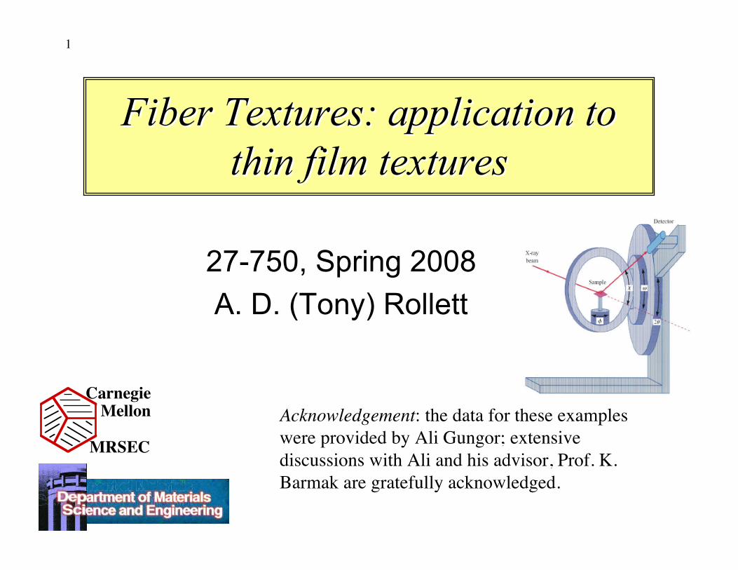
Fiber Textures: application toFiber Textures: application tothin film texturesthin film textures

27-750, Spring 2008A. D. (Tony) Rollett

CarnegieMellon

MRSEC

Acknowledgement: the data for these exampleswere provided by Ali Gungor; extensivediscussions with Ali and his advisor, Prof. K.Barmak are gratefully acknowledged.

2

Lecture ObjectivesLecture Objectives• Give examples of experimental textures of thin copper films;

illustrate the OD representation for a simple case.• Explain (some aspects of) a fiber texture .• Show how to calculate volume fractions associated with each

fiber component from inverse pole figures (from ODF).• Explain use of high resolution pole plots, and analysis of results.• Discuss the phenomenon of axiotaxy - orientation relationships

based on plane-edge matching instead of the usual surfacematching.

• Give examples of the relevance and importance of textures inthin films, such as metallic interconnects, high temperaturesuperconductors and magnetic thin films.

Electromigration Weak Strong IPF VolumeFraction PolePlot Deconvolution

3

SummarySummary• Thin films often exhibit a surprising degree of texture, even when deposited on an

amorphous substrate.• The texture observed is, in general, the result of growth competition between

different crystallographic directions. In fcc metals, e.g., the 111 direction typicallygrows fastest, leading to a preference for this axis to be perpendicular to the filmplane.

• Such a texture is known as a fiber texture because only one axis is preferentiallyaligned whereas the other two are uniformly distributed (“random”).

• Although vapor-deposited films are the most studied, similar considerations applyto electrodeposited films also, which are important in, e.g., copper interconnects.

• Especially in electrodeposition, many different fiber textures can be obtained as afunction of deposition conditions (current density, chemistry of electrolyte etc., orsubstrate temperature, deposition rate).

• Even the crystal structure can vary from the equilibrium one for the conditions.Tantalum is known is known to deposit in a tetragonal form (with a strong 001fiber) instead of BCC, for example.

• Thin film texture should be quantified with Orientation Distributions andvolume fractions, not by deconvolution of peaks in pole figures, or poleplots. The latter approach may look straightforward (and similar to othertypes of analysis of x-ray data) but has many pitfalls.

4

Example 1:Example 1:Interconnect LifetimesInterconnect Lifetimes

• Thin (1 µm or less) metallic lines usedin microcircuitry to connect one part of acircuit with another.

• Current densities (~106 A.cm-2) are veryhigh so that electromigration producessignificant mass transport.

• Failure by void accumulation oftenassociated with grain boundaries


5

SiO2W

linerSiNx

ILD via

Inter-Level-Dielectric

M2

Si substrate

SiO2

M1ILD

SilicideSilicide

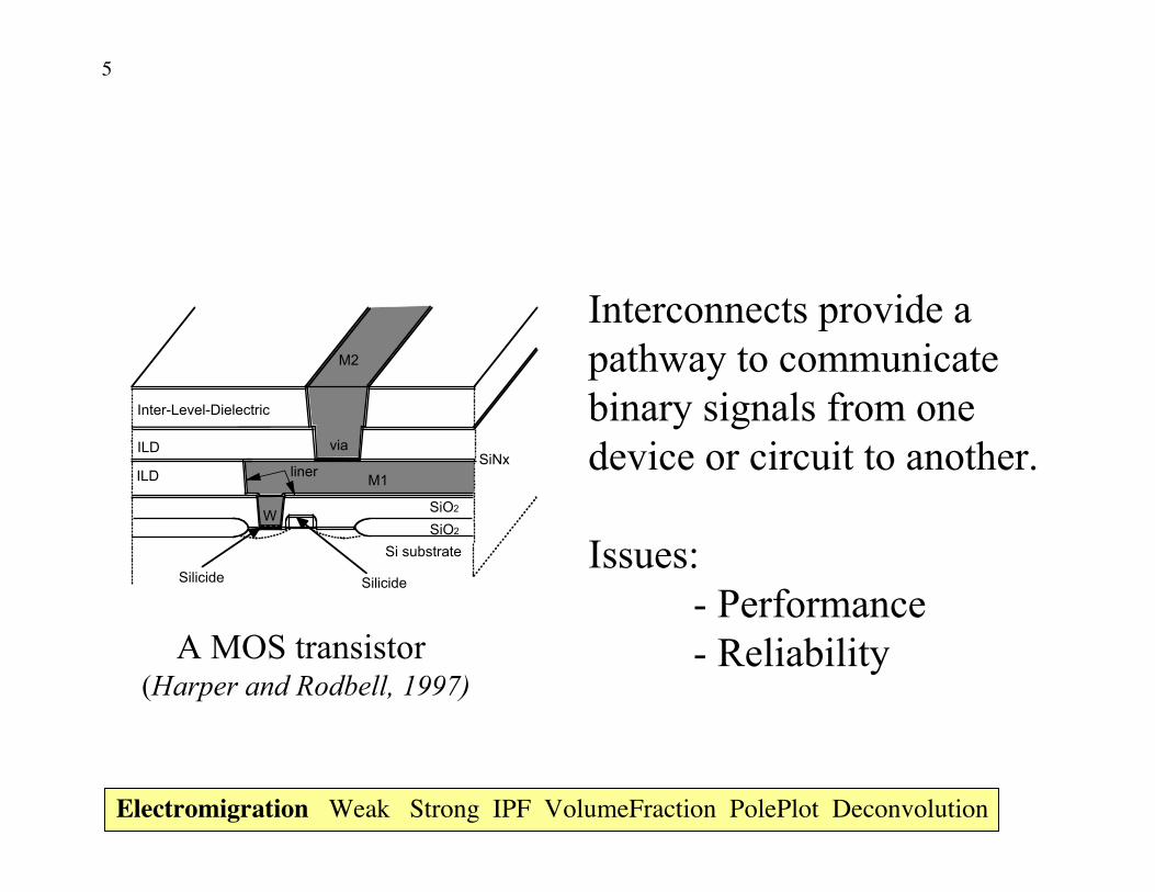
A MOS transistor (Harper and Rodbell, 1997)

Interconnects provide apathway to communicatebinary signals from onedevice or circuit to another.

Issues:- Performance- Reliability


6

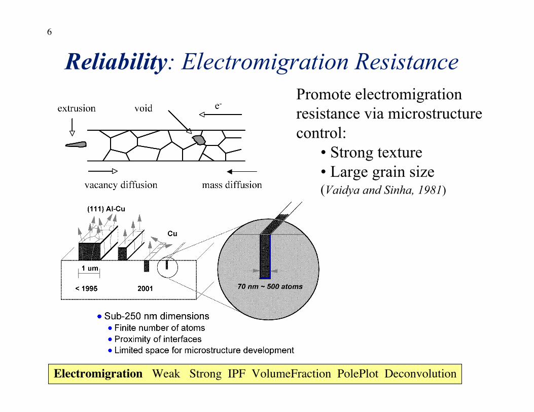
Promote electromigrationresistance via microstructurecontrol:

• Strong texture• Large grain size(Vaidya and Sinha, 1981)

Reliability: Electromigration Resistance


7

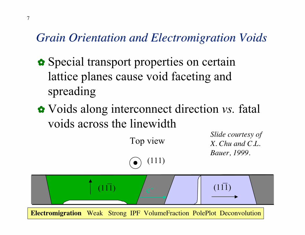
Special transport properties on certainlattice planes cause void faceting andspreading

Voids along interconnect direction vs. fatalvoids across the linewidth

Grain Orientation and Grain Orientation and ElectromigrationElectromigration Voids Voids

(111)

Top view

(111)_

(111)_

e-


Slide courtesy ofX. Chu and C.L.Bauer, 1999.

8

Aluminum Interconnect LifetimeAluminum Interconnect Lifetime

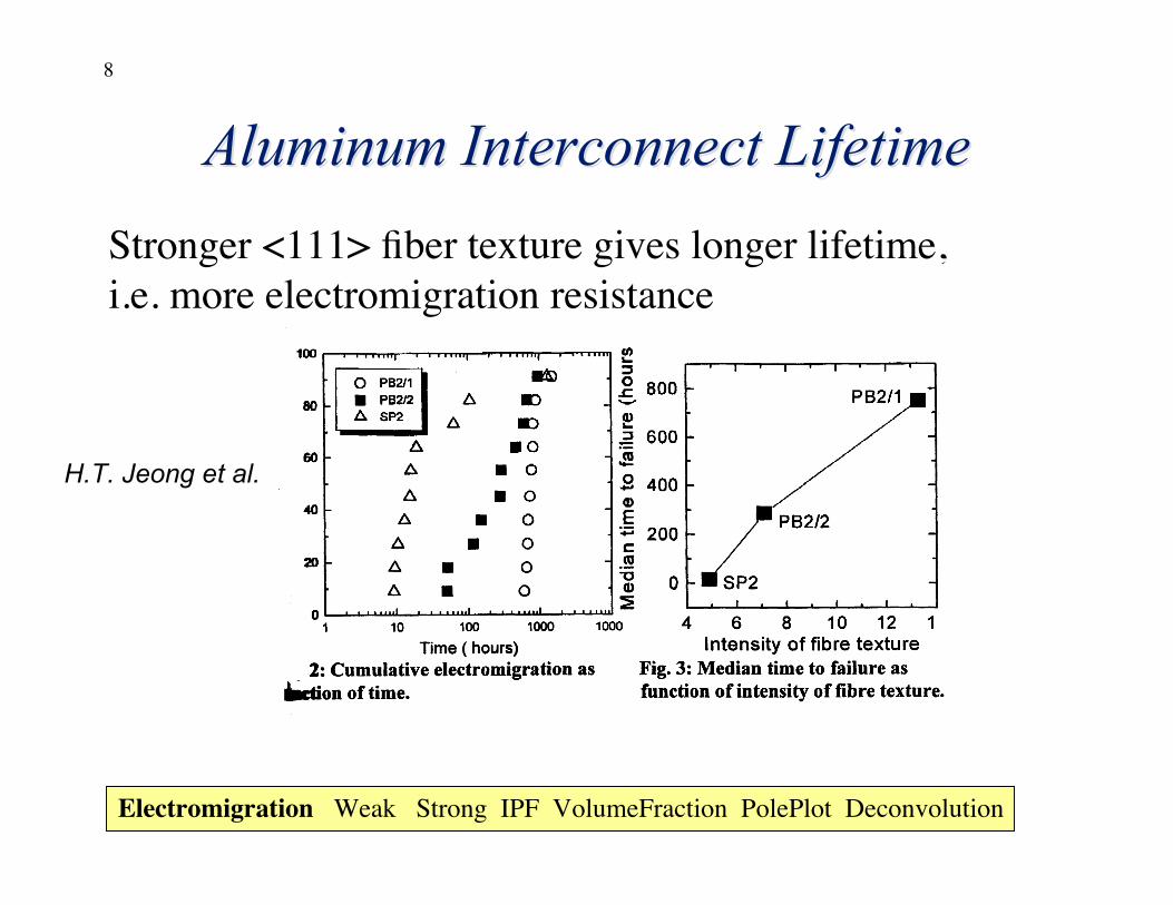
H.T. Jeong et al.

Stronger <111> fiber texture gives longer lifetime, i.e. more electromigration resistance


9

ReferencesReferences• H.T. Jeong et al., “A role of texture and orientation clustering on

electromigration failure of aluminum interconnects,” ICOTOM-12, Montreal, Canada, p 1369 (1999).

• D.B. Knorr, D.P. Tracy and K.P. Rodbell, “Correlation of texturewith electromigration behavior in Al metallization”, Appl. Phys.Lett., 59, 3241 (1991).

• D.B. Knorr, K.P. Rodbell, “The role of texture in theelectromigration behavior of pure Al lines,” J. Appl. Phys., 79,2409 (1996).

• A. Gungor, K. Barmak, A.D. Rollett, C. Cabral Jr. and J.M. E.Harper, “Texture and resistivity of dilute binary Cu(Al), Cu(In),Cu(Ti), Cu(Nb), Cu(Ir) and Cu(W) alloy thin films," J. Vac. Sci.Technology, B 20(6), p 2314-2319 (Nov/Dec 2002).

• Barmak K, Gungor A, Rollett AD, Cabral C, Harper JME. 2003.Texture of Cu and dilute binary Cu-alloy films: impact ofannealing and solute content. Materials Science InSemiconductor Processing 6:175-84.


-> YBCO textures

10

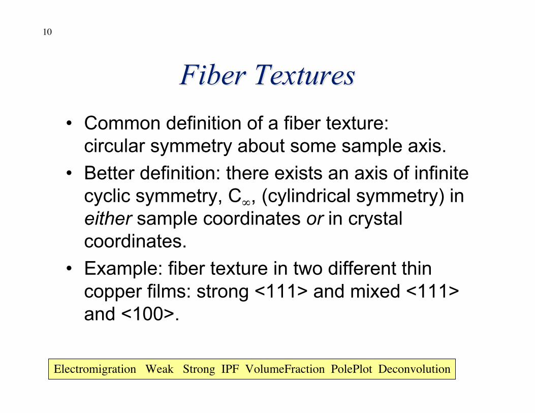
Fiber TexturesFiber Textures• Common definition of a fiber texture:

circular symmetry about some sample axis.• Better definition: there exists an axis of infinite

cyclic symmetry, C∞, (cylindrical symmetry) ineither sample coordinates or in crystalcoordinates.

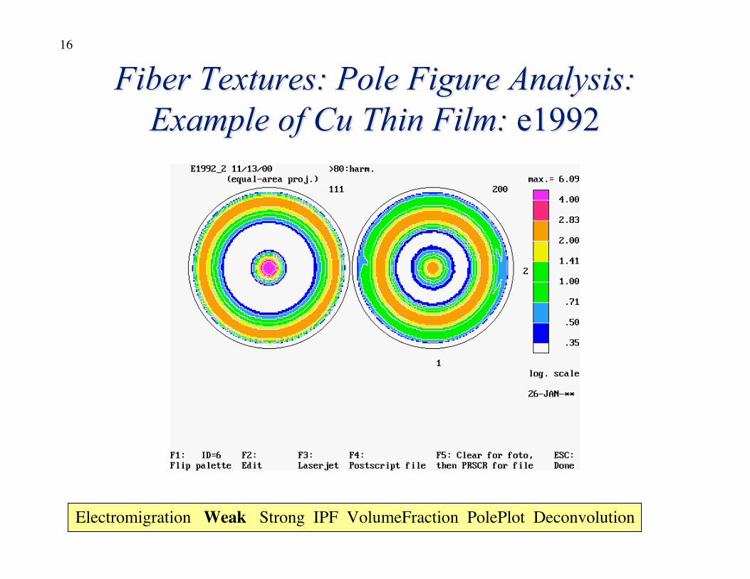
• Example: fiber texture in two different thincopper films: strong <111> and mixed <111>and <100>.


11

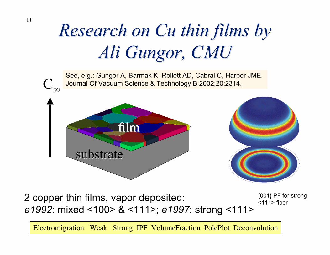
Research on Cu thin films byResearch on Cu thin films byAli Ali GungorGungor, CMU, CMU

substratesubstrate

filmfilm

C∞

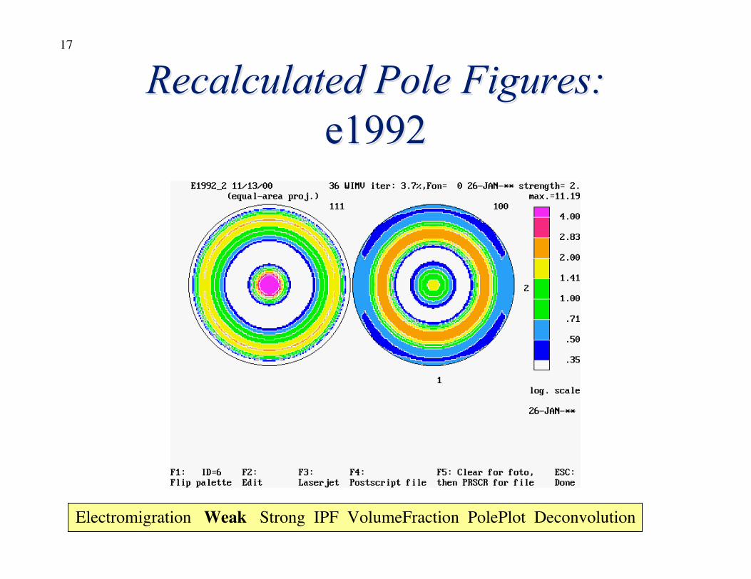
2 copper thin films, vapor deposited:e1992: mixed <100> & <111>; e1997: strong <111>


See, e.g.: Gungor A, Barmak K, Rollett AD, Cabral C, Harper JME. Journal Of Vacuum Science & Technology B 2002;20:2314.

{001} PF for strong<111> fiber

12

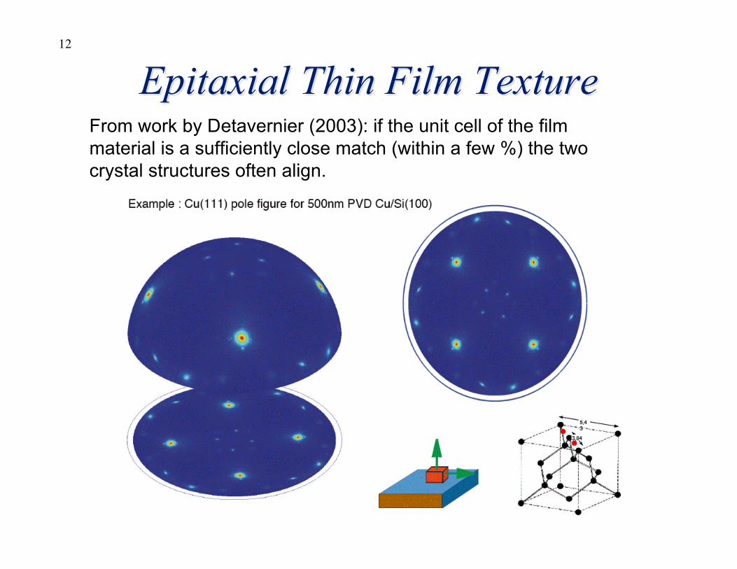
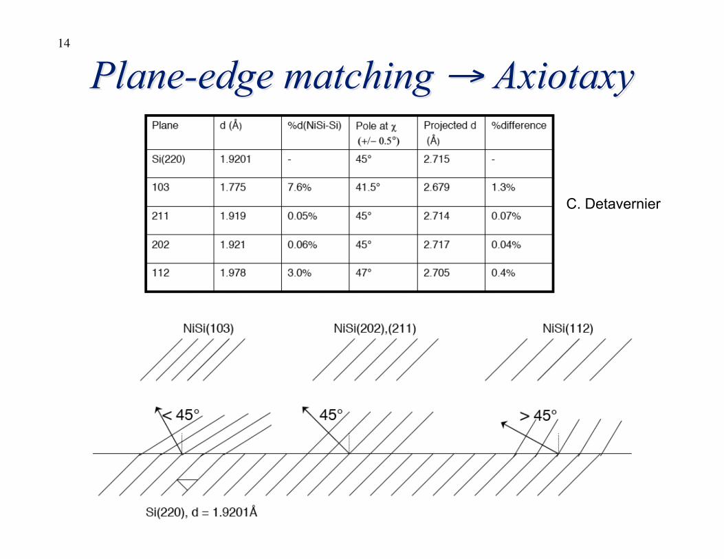
Epitaxial Epitaxial Thin Film TextureThin Film TextureFrom work by Detavernier (2003): if the unit cell of the filmmaterial is a sufficiently close match (within a few %) the twocrystal structures often align.

13

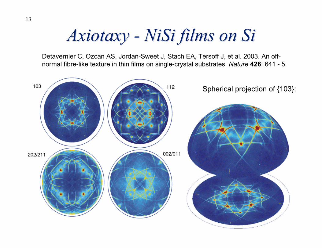
Axiotaxy Axiotaxy - - NiSi NiSi films on films on SiSi

Spherical projection of {103}:

Detavernier C, Ozcan AS, Jordan-Sweet J, Stach EA, Tersoff J, et al. 2003. An off-normal fibre-like texture in thin films on single-crystal substrates. Nature 426: 641 - 5.

14

Plane-edge matching Plane-edge matching →→ AxiotaxyAxiotaxy

C. Detavernier

15

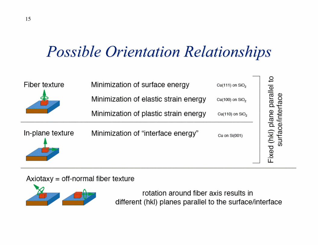
Possible Orientation RelationshipsPossible Orientation Relationships

16

Fiber Textures: Pole Figure Analysis:Fiber Textures: Pole Figure Analysis:Example of Cu Thin Film: Example of Cu Thin Film: e1992e1992


17

Recalculated Pole Figures:Recalculated Pole Figures:e1992e1992


18

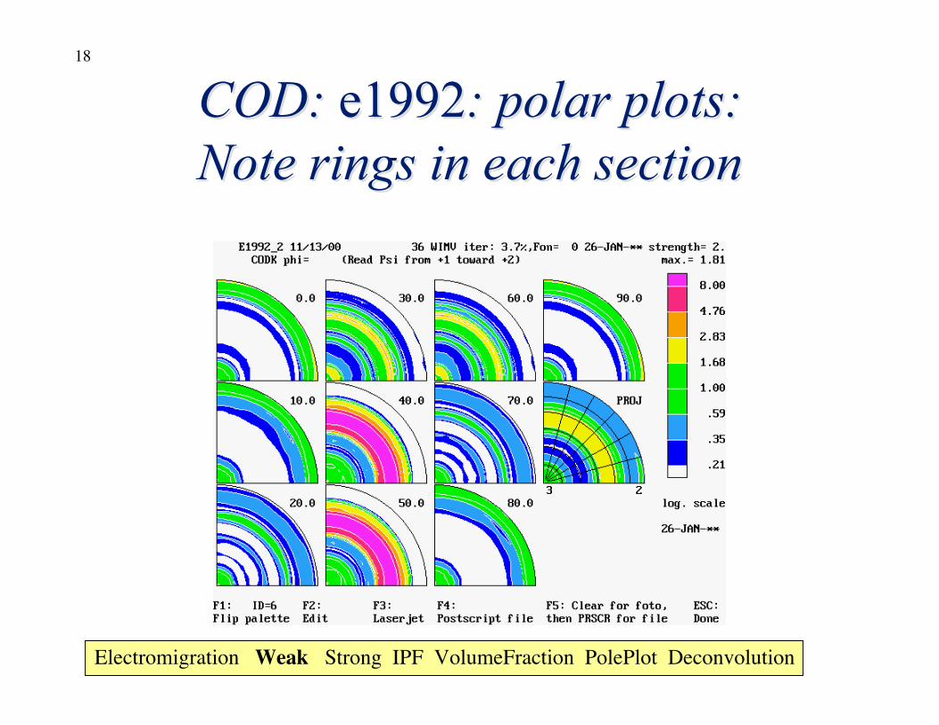
COD: COD: e1992e1992: polar plots:: polar plots:Note rings in each sectionNote rings in each section


19

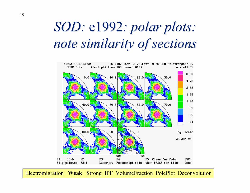
SOD: SOD: e1992e1992: polar plots:: polar plots:note similarity of sectionsnote similarity of sections


20

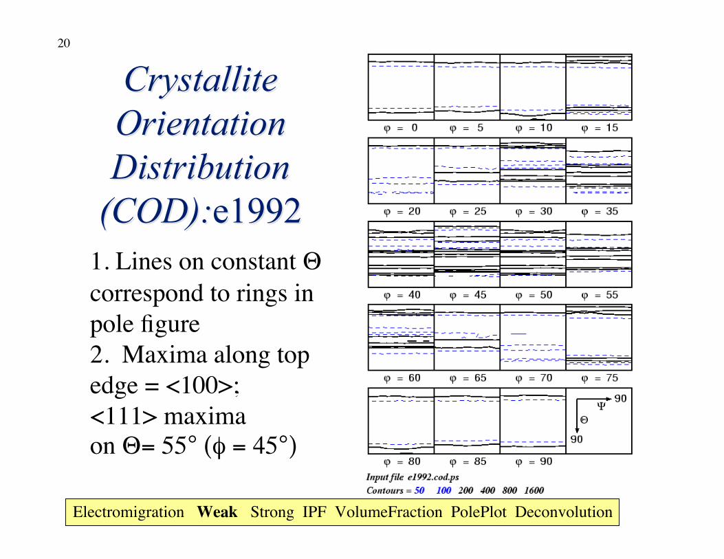
CrystalliteCrystalliteOrientationOrientationDistributionDistribution

(COD):(COD):e1992e19921. Lines on constant Θ correspond to rings inpole figure2. Maxima along top edge = <100>;<111> maxima on Θ= 55° (φ = 45°)


21

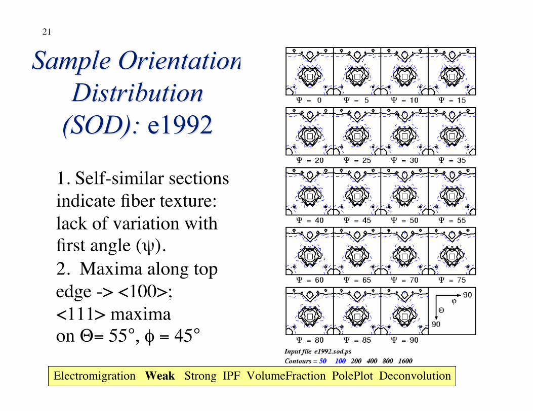
Sample OrientationSample OrientationDistributionDistribution

(SOD): (SOD): e1992e1992

1. Self-similar sectionsindicate fiber texture:lack of variation withfirst angle (ψ).2. Maxima along top edge -> <100>;<111> maxima on Θ= 55°, φ = 45°


22

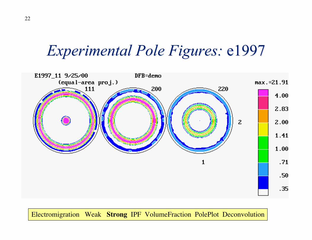
Experimental Pole Figures: Experimental Pole Figures: e1997e1997


23

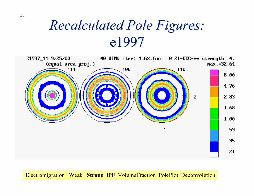
Recalculated Pole Figures:Recalculated Pole Figures:e1997e1997


24

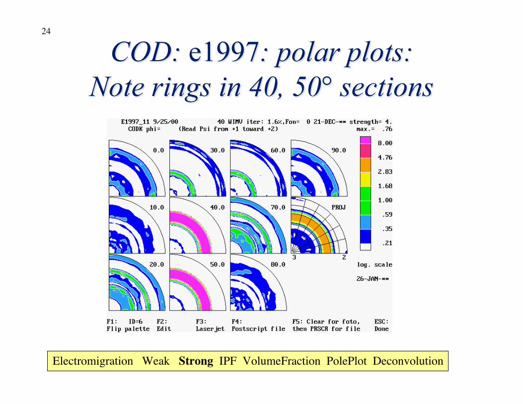
COD: COD: e1997e1997: polar plots:: polar plots:Note rings in 40, 50° sectionsNote rings in 40, 50° sections


25

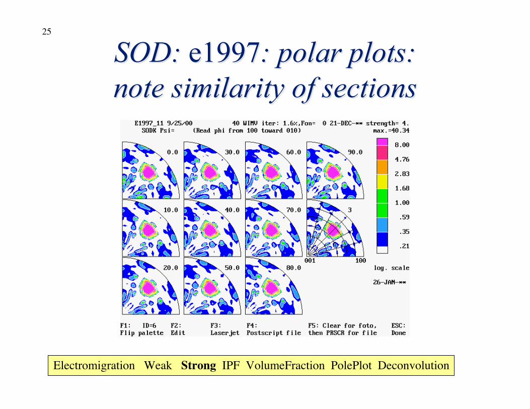
SOD: SOD: e1997e1997: polar plots:: polar plots:note similarity of sectionsnote similarity of sections


26

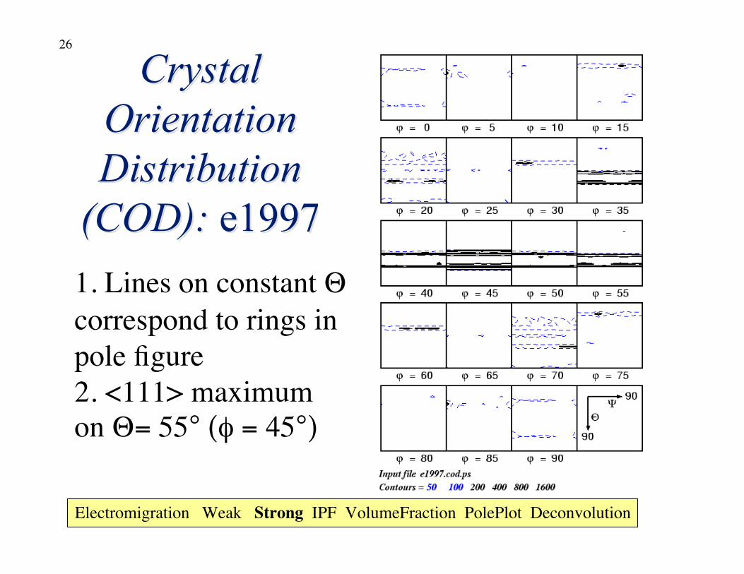
CrystalCrystalOrientationOrientationDistributionDistribution

(COD): (COD): e1997e19971. Lines on constant Θ correspond to rings inpole figure2. <111> maximumon Θ= 55° (φ = 45°)


27

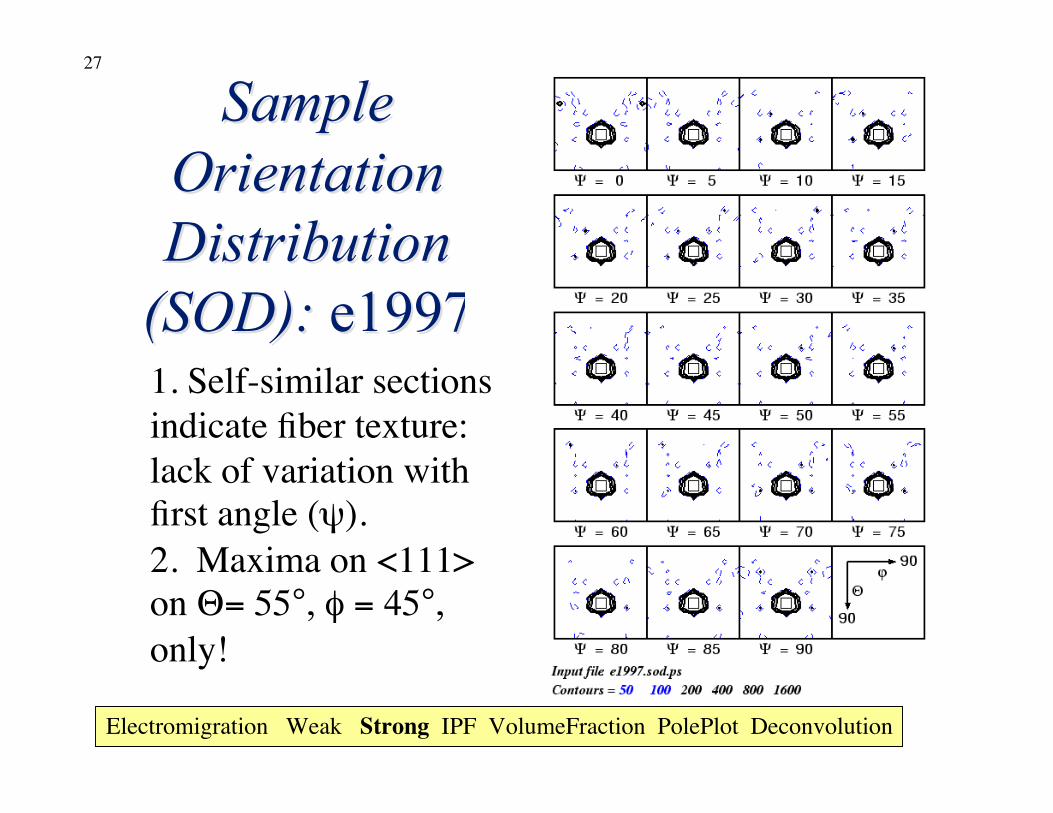
SampleSampleOrientationOrientationDistributionDistribution

(SOD): (SOD): e1997e19971. Self-similar sectionsindicate fiber texture:lack of variation withfirst angle (ψ).2. Maxima on <111> on Θ= 55°, φ = 45°,only!


28

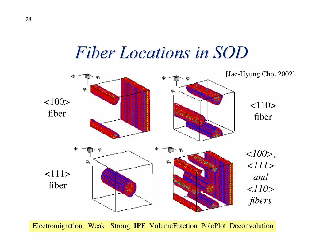
Fiber Locations in SODFiber Locations in SOD

<100>fiber

<111>fiber

<110>fiber

<100>,<111>

and<110>fibers

[Jae-Hyung Cho, 2002]


29

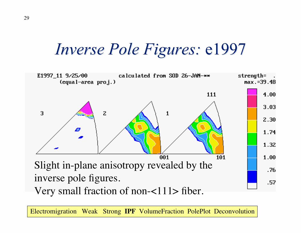
Inverse Pole Figures: Inverse Pole Figures: e1997e1997

Slight in-plane anisotropy revealed by theinverse pole figures.Very small fraction of non-<111> fiber.


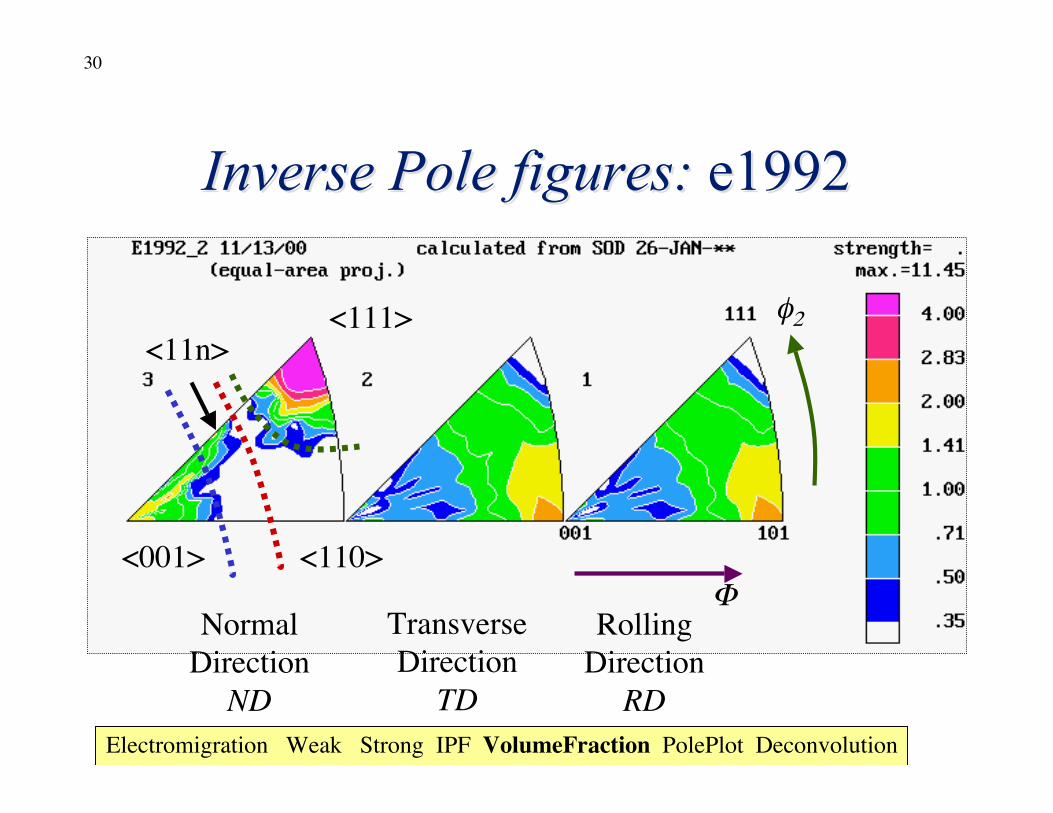
30

Inverse Pole figures: Inverse Pole figures: e1992e1992

<111><11n>

<001> <110>Φ

φ2

NormalDirection

ND

TransverseDirection

TD

RollingDirection

RDElectromigration Weak Strong IPF VolumeFraction PolePlot Deconvolution

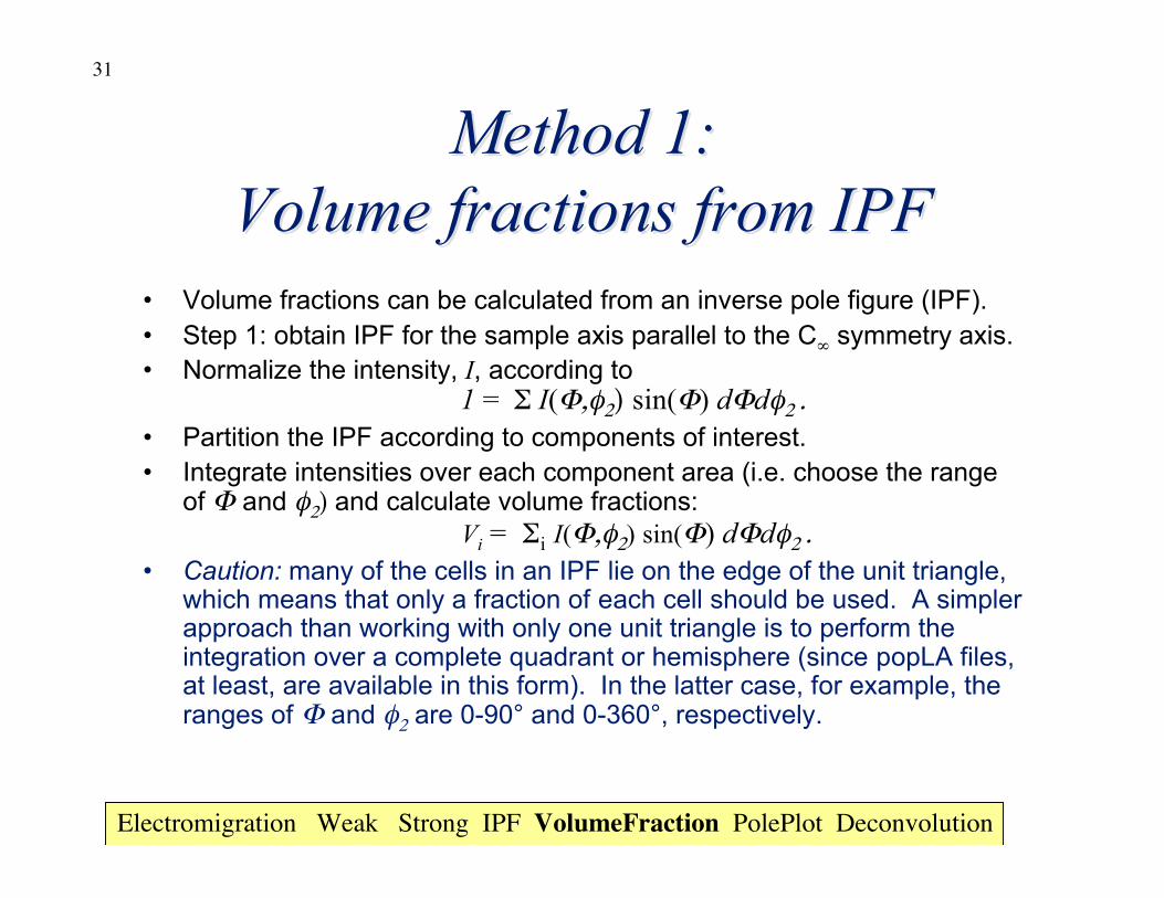
31

Method 1:Method 1:Volume fractions from IPFVolume fractions from IPF

• Volume fractions can be calculated from an inverse pole figure (IPF).• Step 1: obtain IPF for the sample axis parallel to the C∞ symmetry axis.• Normalize the intensity, I, according to

1 = Σ I(Φ,φ2) sin(Φ) dΦdφ2 .• Partition the IPF according to components of interest.• Integrate intensities over each component area (i.e. choose the range

of Φ and φ2) and calculate volume fractions: Vi = Σi I(Φ,φ2) sin(Φ) dΦdφ2 .

• Caution: many of the cells in an IPF lie on the edge of the unit triangle,which means that only a fraction of each cell should be used. A simplerapproach than working with only one unit triangle is to perform theintegration over a complete quadrant or hemisphere (since popLA files,at least, are available in this form). In the latter case, for example, theranges of Φ and φ2 are 0-90° and 0-360°, respectively.


32

Volume fractions from IPFVolume fractions from IPF• How to measure distance from a component in an inverse pole

figure?- This is simpler than for general orientations because we areonly comparing directions (on the sphere).- Therefore we can use the dot (scalar) product: if we have afiber axis, e.g. f = [211], and a general cell denoted by n, wetake f•b (and, clearly use cos-1 if we want an angle). The nearerthe value of the dot product is to +1, the closer are the twodirections.

• Symmetry: as for general orientations one must take account ofsymmetry. However, it is sensible to simplify by using sets ofsymmetrically related points in the upper hemisphere for eachfiber axis, e.g. {100,-100,010,0-10,001}. Be aware that thereare 24 equivalent points for a general direction (not coincidentwith a symmetry element).

33

Method 2: Pole plotsMethod 2: Pole plots

• If a perfect fiber exists then it is enough to scan overthe tilt angle only and make a pole plot.

• A “perfect fiber” means that the intensity in all polefigures is in the form of rings with uniform intensitywith respect to azimuth (C∞, aligned with the filmplane normal).

• High resolution is then feasible, compared tostandard 5°x5° pole figures, e.g 0.1°.

• High resolution inverse PF preferable but notmeasurable.


34

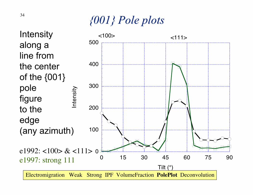
Intensityalong aline fromthe centerof the {001}polefigureto theedge(any azimuth)

e1992: <100> & <111>e1997: strong 111

0

100

200

300

400

500

0 15 30 45 60 75 90

Inte

nsity

Tilt (°)

<100> <111>


{001} Pole plots{001} Pole plots

35

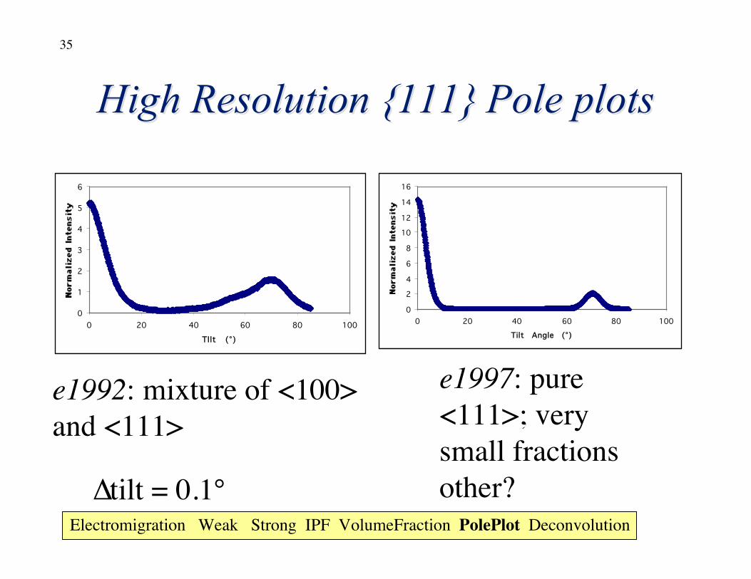
High Resolution {111} Pole plotsHigh Resolution {111} Pole plots

0

2

4

6

8

10

12

14

16

0 20 40 60 80 100

Tilt Angle (°)

0

1

2

3

4

5

6

0 20 40 60 80 100

TIlt (°)

e1992: mixture of <100>and <111>

e1997: pure<111>; verysmall fractionsother?∆tilt = 0.1°


36

Volume fractionsVolume fractions

• Pole plots (1D variation of intensity):If regions in the plot can be identified as beinguniquely associated with a particular volume fraction,then an integration can be performed to find an areaunder the curve.

• The volume fraction is then the sum of the associatedareas divided by the total area.

• Else, deconvolution required, which, unfortunately, isthe usual case.

• In other words, this method is only reasonable to useif the only components are a single fiber texture anda random background.


37

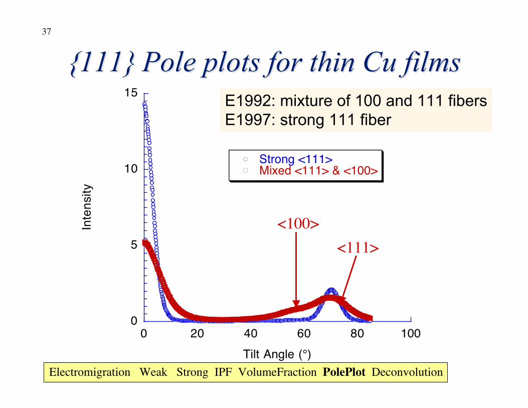
{111} Pole plots for thin Cu films{111} Pole plots for thin Cu films

0

5

10

15

0 20 40 60 80 100

Strong <111>Mixed <111> & <100>

Inte

nsity

Tilt Angle (°)

<100><111>


E1992: mixture of 100 and 111 fibersE1997: strong 111 fiber

38

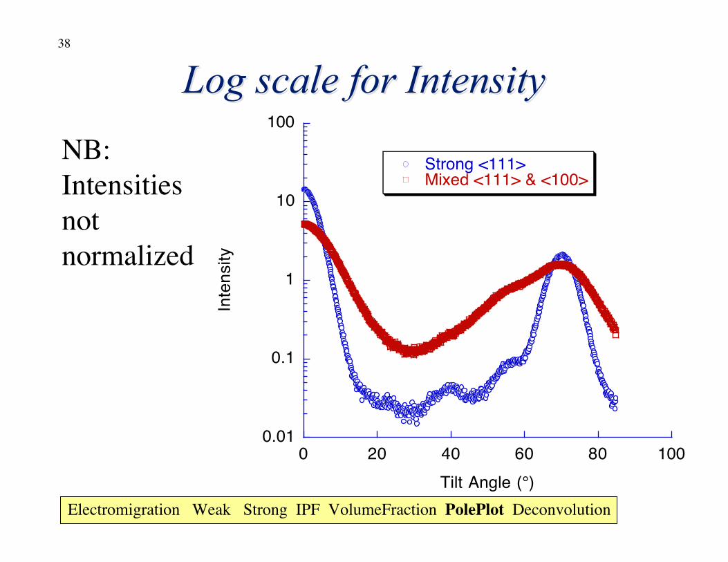
Log scale for IntensityLog scale for Intensity

0.01

0.1

1

10

100

0 20 40 60 80 100

Strong <111>Mixed <111> & <100>

Inte

nsity

Tilt Angle (°)

NB:Intensitiesnotnormalized


39

Area under the CurveArea under the Curve

• Tilt Angle equivalent to second Eulerangle, θ ≡ Φ • Requirement: 1 = Σ I(θ) sin(θ) dθ;

θ measured in radians.• Intensity as supplied not normalized.• Problem: data only available to 85°: therefore correct for finite range.• Defocusing neglected.


40

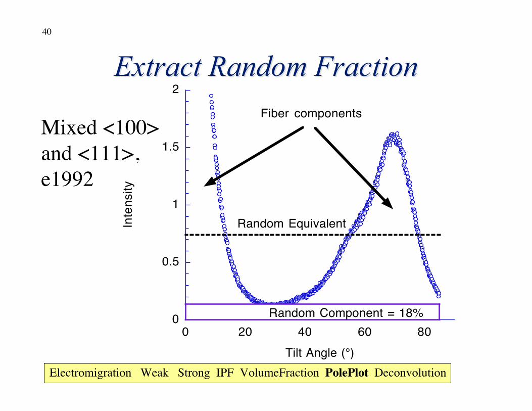
Extract Random FractionExtract Random Fraction

0

0.5

1

1.5

2

0 20 40 60 80

e1992.111PF.data

Inte

nsity

Tilt Angle (°)

Random Component = 18%

Fiber components

Random Equivalent

Mixed <100>and <111>,e1992


41

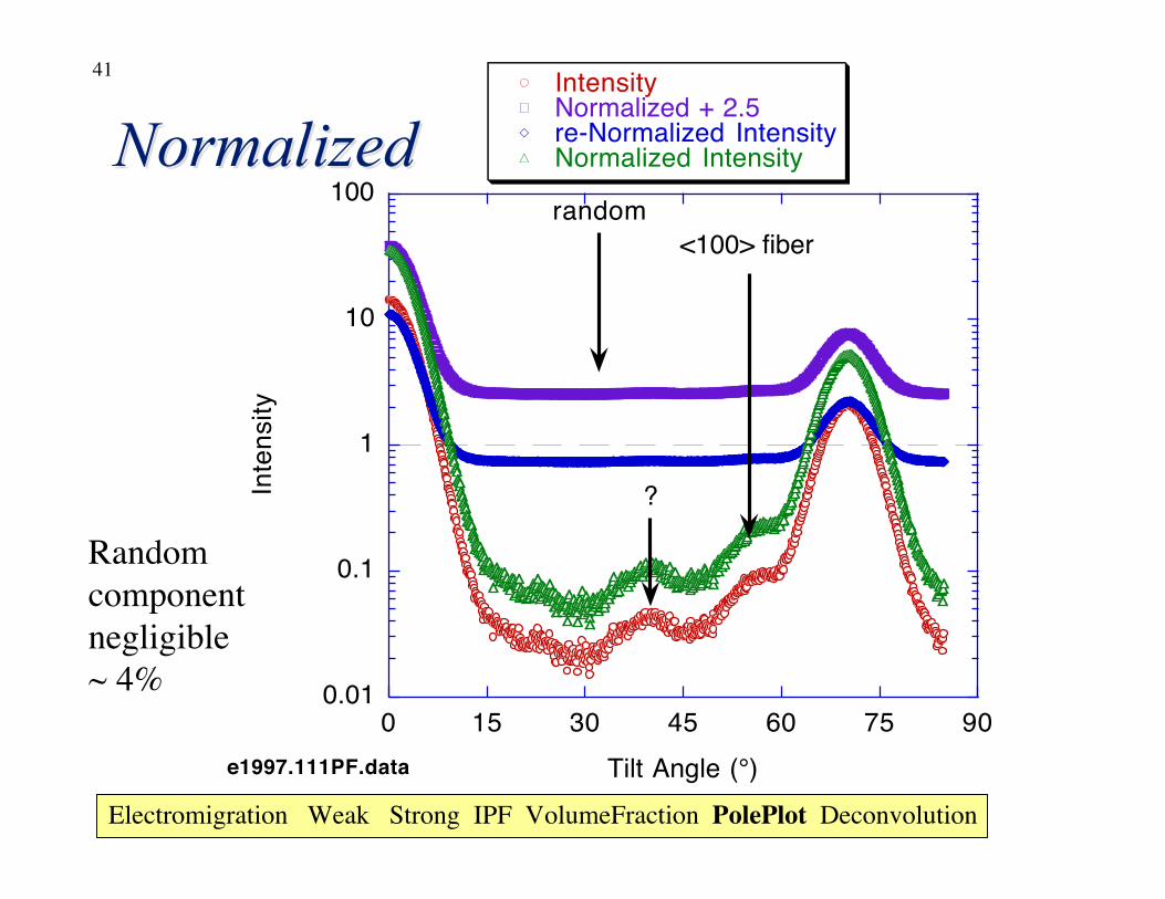
NormalizedNormalized

0.01

0.1

1

10

100

0 15 30 45 60 75 90

e1997.111PF.data

IntensityNormalized + 2.5re-Normalized IntensityNormalized Intensity

Inte

nsity

Tilt Angle (°)

<100> fiber

random

?

Randomcomponentnegligible~ 4%


42

DeconvolutionDeconvolution

• Method is based on identifying eachpeak in the pole plot, fitting a Gaussianto it, and then checking the sum of theindividual components for agreementwith the experimental data.

• Areas under each peak are calculated.• Corrections must be made for

multiplicities.


43

0 20 40 60 80

0

20

40

60

80

100

120

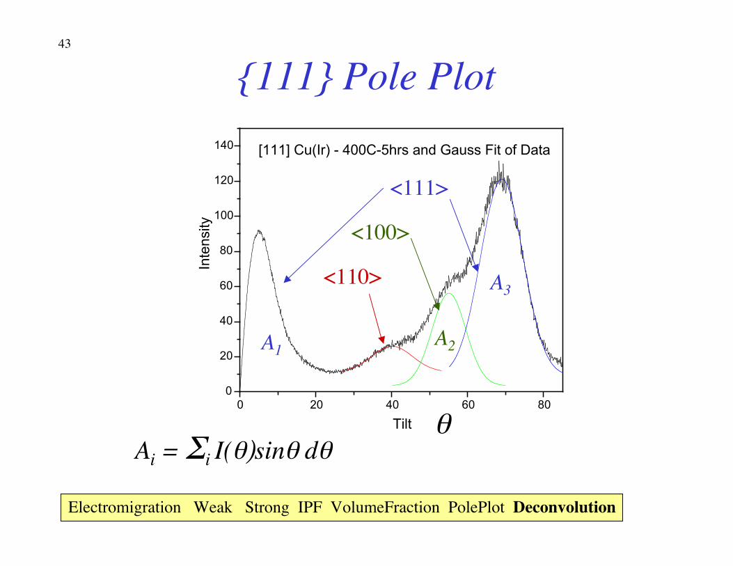
140 [111] Cu(Ir) - 400C-5hrs and Gauss Fit of Data

Inte

nsity

Tilt

<111>

<100>

<110>

{111} Pole Plot

A1A2

A3

θAi = Σi I(θ)sinθ dθ


44

0 10 20 30 40 50 60 70 80

0

20

40

60

80

100

120

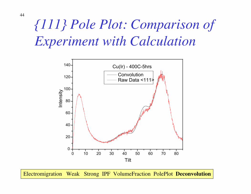
140 Cu(Ir) - 400C-5hrs

Inte

nsity

Tilt

Convolution Raw Data <111>

{111} Pole Plot: Comparison ofExperiment with Calculation


45

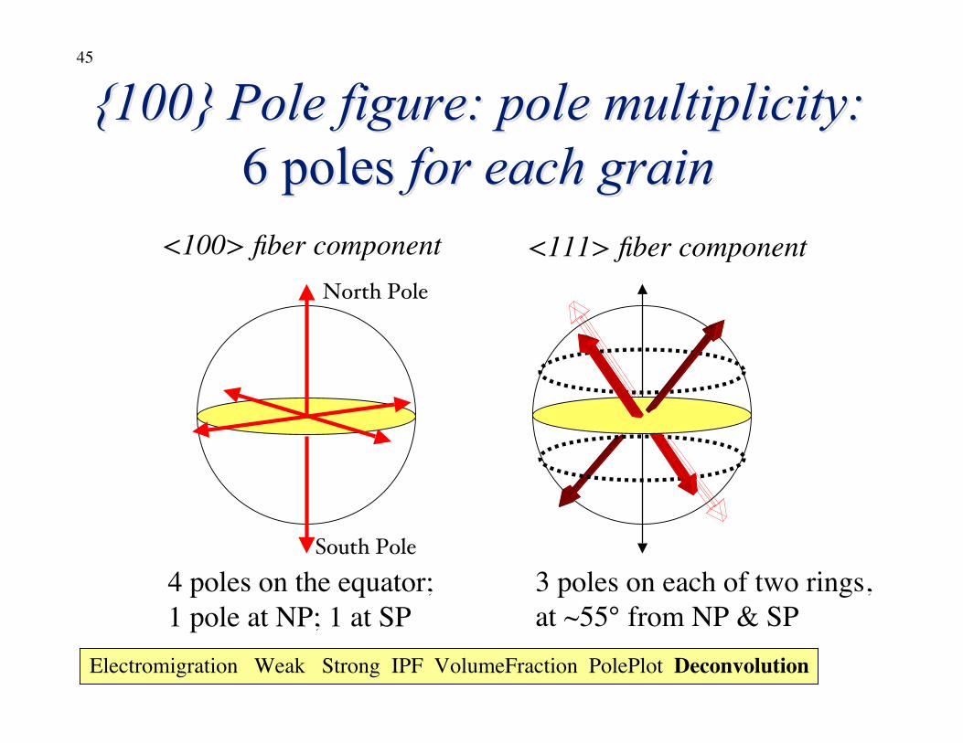
{100} Pole figure: pole multiplicity:{100} Pole figure: pole multiplicity:6 poles 6 poles for each grainfor each grain

<100> fiber component <111> fiber component

4 poles on the equator;1 pole at NP; 1 at SP

3 poles on each of two rings, at ~55° from NP & SP

North Pole

South Pole


46

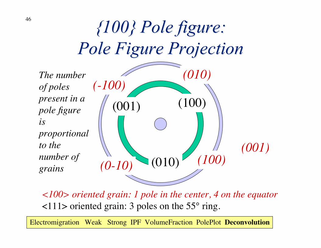
{100} Pole figure:{100} Pole figure:Pole Figure ProjectionPole Figure Projection

(100)

(010)

(001)

(001)(100)

(010)(-100)

(0-10)

<100> oriented grain: 1 pole in the center, 4 on the equator<111> oriented grain: 3 poles on the 55° ring.

The numberof polespresent in apole figureisproportionalto thenumber ofgrains


47

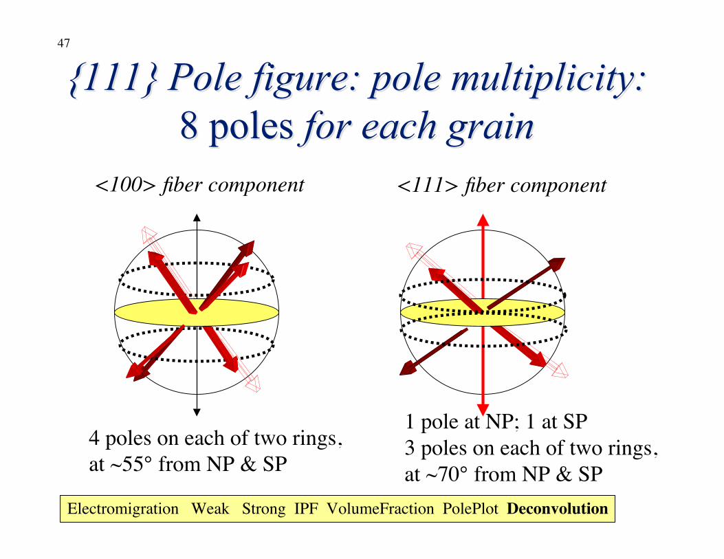
{111} Pole figure: pole multiplicity:{111} Pole figure: pole multiplicity:8 poles 8 poles for each grainfor each grain

<111> fiber component

1 pole at NP; 1 at SP3 poles on each of two rings, at ~70° from NP & SP

4 poles on each of two rings, at ~55° from NP & SP

<100> fiber component


48

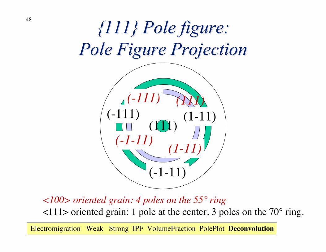
{111} Pole figure:{111} Pole figure:Pole Figure ProjectionPole Figure Projection

(001)

<100> oriented grain: 4 poles on the 55° ring<111> oriented grain: 1 pole at the center, 3 poles on the 70° ring.

(-1-11)

(1-11)(111)

(1-11)

(111)(-111)

(-1-11)

(-111)


49

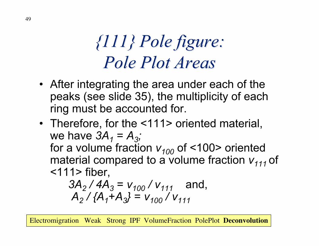
{111} Pole figure:{111} Pole figure:Pole Plot AreasPole Plot Areas

• After integrating the area under each of thepeaks (see slide 35), the multiplicity of eachring must be accounted for.

• Therefore, for the <111> oriented material,we have 3A1 = A3;for a volume fraction v100 of <100> orientedmaterial compared to a volume fraction v111 of<111> fiber,

3A2 / 4A3 = v100 / v111 and, A2 / {A1+A3} = v100 / v111


50

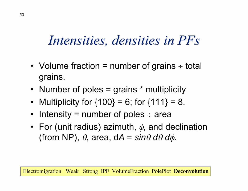
Intensities, densities in Intensities, densities in PFsPFs

• Volume fraction = number of grains ÷ totalgrains.

• Number of poles = grains * multiplicity• Multiplicity for {100} = 6; for {111} = 8.• Intensity = number of poles ÷ area• For (unit radius) azimuth, φ, and declination

(from NP), θ, area, dA = sinθ dθ dφ.


51

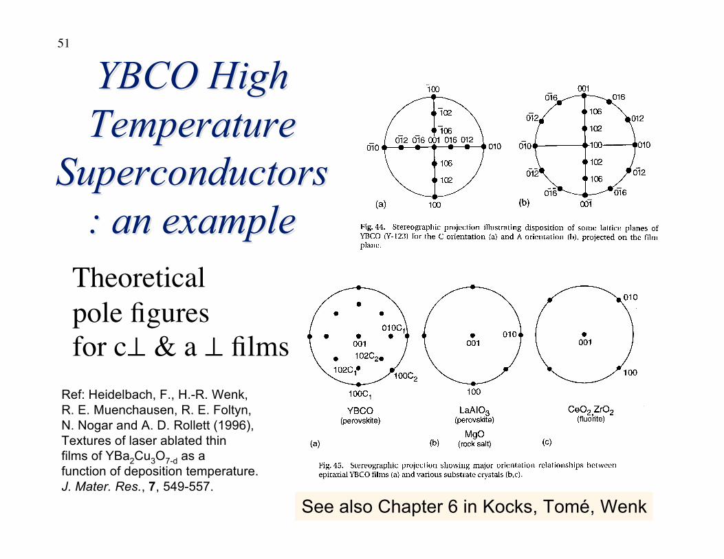
YBCO HighYBCO HighTemperatureTemperature

SuperconductorsSuperconductors: an example: an example

Theoreticalpole figuresfor c⊥ & a ⊥ films

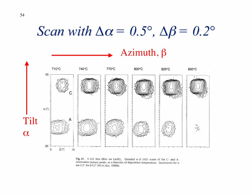
Ref: Heidelbach, F., H.-R. Wenk, R. E. Muenchausen, R. E. Foltyn, N. Nogar and A. D. Rollett (1996), Textures of laser ablated thin films of YBa2Cu3O7-d as a function of deposition temperature. J. Mater. Res., 7, 549-557.

See also Chapter 6 in Kocks, Tomé, Wenk

52

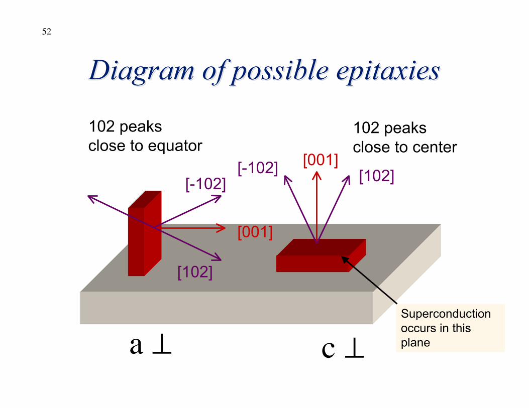
Diagram of possible Diagram of possible epitaxiesepitaxies

[001]

[001]

[102][-102][-102]

[102]

c ⊥a ⊥

102 peaksclose to equator

102 peaksclose to center

Superconductionoccurs in thisplane

53

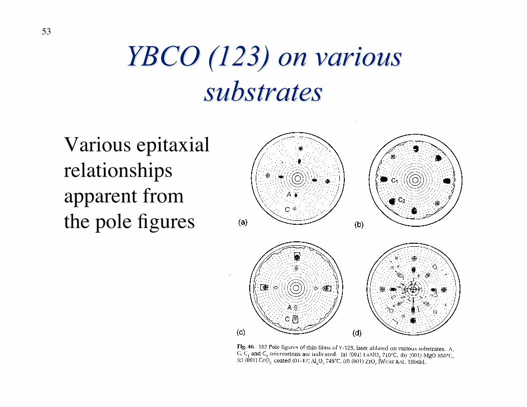
YBCO (123) on variousYBCO (123) on varioussubstratessubstrates

Various epitaxialrelationshipsapparent fromthe pole figures

54

Scan with Scan with ∆∆αα = 0.5°, = 0.5°, ∆∆ββ = 0.2° = 0.2°

Tiltα

Azimuth, β

55

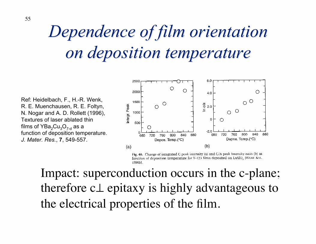
Dependence of film orientationDependence of film orientationon deposition temperatureon deposition temperature

Impact: superconduction occurs in the c-plane;therefore c⊥ epitaxy is highly advantageous tothe electrical properties of the film.

Ref: Heidelbach, F., H.-R. Wenk, R. E. Muenchausen, R. E. Foltyn, N. Nogar and A. D. Rollett (1996), Textures of laser ablated thin films of YBa2Cu3O7-d as a function of deposition temperature. J. Mater. Res., 7, 549-557.

56

Summary: Fiber TexturesSummary: Fiber Textures• Extraction of volume fractions possible provided that

fiber texture established.• Fractions from IPF simple but resolution limited by

resolution of OD.• Pole plot shows entire texture.• Random fraction can always be extracted.• Specific fiber components may require

deconvolution when the peaks overlap; notadvisable when more than one component ispresent (or, great care required).

• Calculation of volume fraction from pole figures/plotsassumes that all corrections have been correctlyapplied (background subtraction, defocussing,absorption).

57

Summary: other issuesSummary: other issues• If epitaxy of any kind occurs between a film and its substrate,

the (inevitable) difference in lattice paramter(s) will lead toresidual stresses. Differences in thermal expansion willreinforce this.

• Residual stresses broaden diffraction peaks and may distort theunit cell (and lower the crystal symmetry), particularly if a highdegree of epitaxy exists.

• Mosaic spread, or dispersion in orientation is always of interest.In epitaxial films, one may often assume a Gaussian distributionabout an ideal component and measure the standard deviationor full-width-half-maximum (FWHM).

• Off-axis alignment is also possible, which is known as axiotaxy.

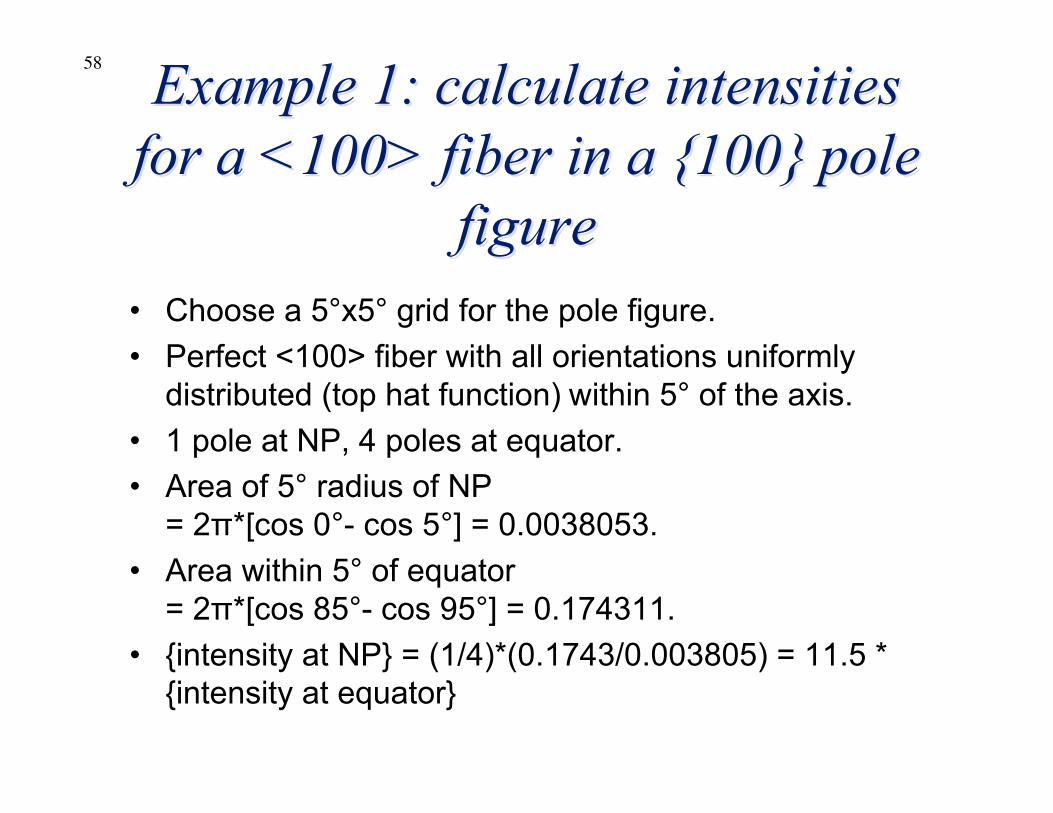
58 Example 1: calculate intensitiesExample 1: calculate intensitiesfor a <100> fiber in a {100} polefor a <100> fiber in a {100} pole

figurefigure• Choose a 5°x5° grid for the pole figure.• Perfect <100> fiber with all orientations uniformly

distributed (top hat function) within 5° of the axis.• 1 pole at NP, 4 poles at equator.• Area of 5° radius of NP

= 2π*[cos 0°- cos 5°] = 0.0038053.• Area within 5° of equator

= 2π*[cos 85°- cos 95°] = 0.174311.• {intensity at NP} = (1/4)*(0.1743/0.003805) = 11.5 *

{intensity at equator}

59

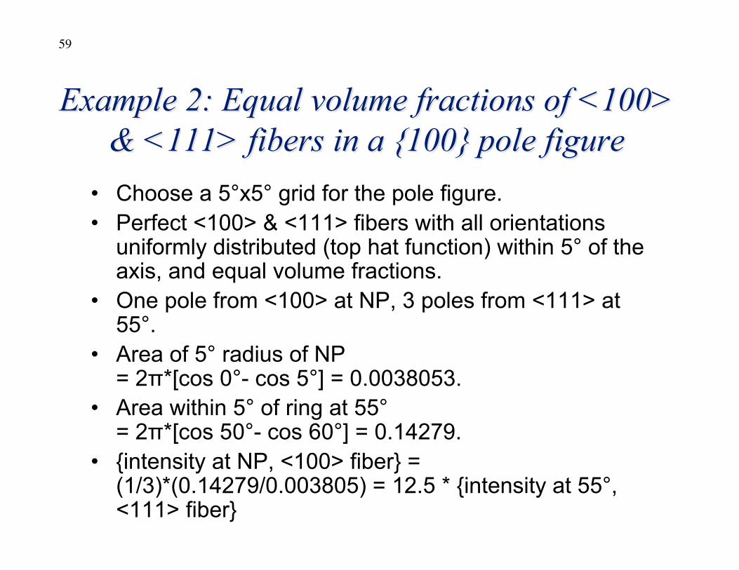
Example 2: Equal volume fractions of <100>Example 2: Equal volume fractions of <100>& <111> fibers in a {100} pole figure& <111> fibers in a {100} pole figure

• Choose a 5°x5° grid for the pole figure.• Perfect <100> & <111> fibers with all orientations

uniformly distributed (top hat function) within 5° of theaxis, and equal volume fractions.

• One pole from <100> at NP, 3 poles from <111> at55°.

• Area of 5° radius of NP= 2π*[cos 0°- cos 5°] = 0.0038053.

• Area within 5° of ring at 55°= 2π*[cos 50°- cos 60°] = 0.14279.

• {intensity at NP, <100> fiber} =(1/3)*(0.14279/0.003805) = 12.5 * {intensity at 55°,<111> fiber}

Documents

Fiber Textures: application to thin film texturespajarito.materials.cmu.edu/...ThinFilm...Mar08.pdf · Fiber Textures: application to thin film textures 27-750, Spring 2008 A. D