Field Description Using Aerial Images

Alexandre Jose Cordeiro Lealalexandre.leal@tecnico.ulisboa.pt

Instituto Superior Tecnico, Universidade de Lisboa, Lisboa, Portugal

November 2018

Abstract

The sustainability topic has been debated in the last decades, with the agricultural developmentbeing of the utmost importance. Precision agriculture is increasingly practiced, consisting on a setof digital tools to monitor agricultural processes. The aim of this work is to develop algorithms toautomatically classify the land cover. The object of study are high-resolution RGB aerial images,belonging to two times of the year, obtained with the aid of an UAV. The images represent anagro-silvo-pastoral rainfed system, where the classes of interest are trees, shadows and soil. The soilclass includes the bare ground and the pastures. Four classification methods were developed, allwith a common stage, where regions of interest for classification are generated. The first method,heuristic, resorts to computer vision tools. The remaining are learning-based methods. One of themuses texture and colour features to describe the regions of interest, using a Support Vector Machine(SVM) as a classifier. In the others, a pre-trained convolutional neural network is used. In one of them,this network is adapted to the problem under study. In the other, the network is used to extract afeature vector that describes the objects of interest, then being used a SVM for the classification. Thelearning-based methods present better results than the heuristic one. The best performance is achievedby the method that uses the SVM to classify regions of interest according to texture and colour, withan accuracy of 93.06% and a F-score of 0.844.Keywords: precision agriculture, aerial imagery, image processing, segmentation, feature extraction,machine learning.

1. Introduction

One of today’s major concerns is the sustainabil-ity matter. The world is sustainable if the actualgenerations are capable of providing the necessaryresources to the upcoming ones, so that they havean average life quality, at least. This concept isvery extensive, with different areas interrelated, asin the case of agriculture, that needs to adapt forthe future. Therefore, agriculture sustainability isof utter importance, for instance to aid on endingpoverty and hunger, or dealing with the climatechanges. By 2050, the population is expected toincrease significantly. The global demand for foodwill consequently raise, but also for other resources,such as water or minerals. The implementation ofresilient agriculture practices is crucial, as well asthe investment in agricultural research and exten-sion services. Farmers will have to produce morefood per unit of land, water, and agrochemicals [2].

Precision agriculture is a type of agriculture thatis becoming increasingly relevant over the years. Itis a type of farming that makes use of digital tech-niques for monitoring and optimizing the agricul-tural production processes [6]. Monitoring is done

by acquiring constant information about spatial andtemporal variations in the field. Then, data collec-tion allows obtaining a field variability mapping,from which the decision making is done. At last,the management practice is put to work, on thefield itself. The ultimate goal is to yield maximiza-tion with minimal inputs. It aids on fertilization,irrigation [1], or to understand the crop height. Re-mote sensing techniques on precision agriculture arevery popular these days, by means of UAVs or satel-lites. The acquisition of information is improvedwith the technological developments on tools suchas the Global Position Systems (GPSs), Geograph-ical Information Systems (GISs), or cameras. Thisnovel type of agriculture coupes two major topics ofcomputer science, computer vision and intelligentsystems.

This work is related to the investigation projectsof TerraPrima, a spin-off of Instituto Superior Tc-nico, mainly focused on the conception and imple-mentation of integrated systems in the field of man-agement agriculture [9]. They do consulting in areasdesignated as agro-silvopastorals rainfed systems,occupied by cork and/or holm oaks. The main tar-

1

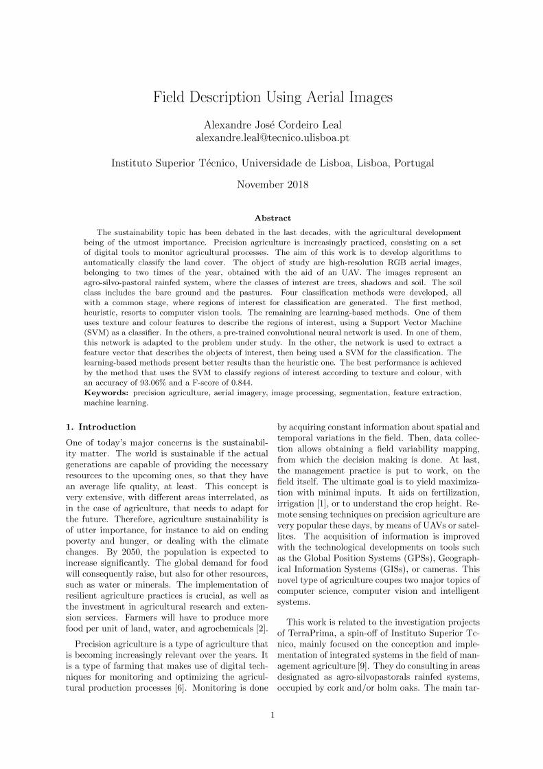
get of this work is to develop a solution that is ableto automatically analyze and classify the occupa-tion of a farmstead land cover. A set of 14 UAVaerial images, from a farmstead close to a villagenamed Cabeo de Vide, Fronteira, Portugal, consti-tute the object of study. Three classes of interestare analyzed: shadows, trees and soil. The soil classincludes both the herbaceous and bare ground. Thephotos belong to two different flights, dating fromNovember 2017 (images named Nov-1 to Nov-9) andJanuary 2018 (images named Jan-1 to Jan-5). Fig-ure 1 provides an example of each.

(a) Image Nov-1 (b) Image Jan-3

Figure 1: Example images from each flight.

At the time of the first flight, the absence of rainmade the herbaceous dry, leading to a bigger con-trast between the soil class and the remaining, asone can see in Figure 1(a). At the time of the sec-ond flight, the herbaceous were more verdant, andthe colour variability between trees and soil dimin-ished, leading to an inter-class similarity, as shownin Figure 1(b). Intra-class and inter-class variabilityconcepts are very meaningful. For instance, com-paring the soil from Figure 1(a) with the one fromFigure 1(b), these are quite dissimilar, resulting ina higher intra-class variability.

To solve the problem under analysis, four differ-ent methodologies were implemented. These have acommon stage, a segmentation procedure, in whichthe input images are divided into regions of inter-est, leading to an object-based analysis. The firstmethod is a non-learning-based one, resorting tocomputer vision tools - Computer Vision Heuristic.The remaining three are learning-based methods.The first method, named as SVM, consists on train-ing a SVM model with a set of selected features,extracted from the regions of interest. The secondis designated as CNN, in which is applied a fine-tuning technique on a pre-trained CNN. The lastis a hybrid approach, named CNN-SVM, in whicha set of features extracted from a pre-trained CNNare used to train a SVM.

2. Computer Vision HeuristicThis chapter describes the implementation of theComputer Vision Heuristic algorithm.

As mentioned, the four methodologies proposedhave a common stage, a segmentation process that

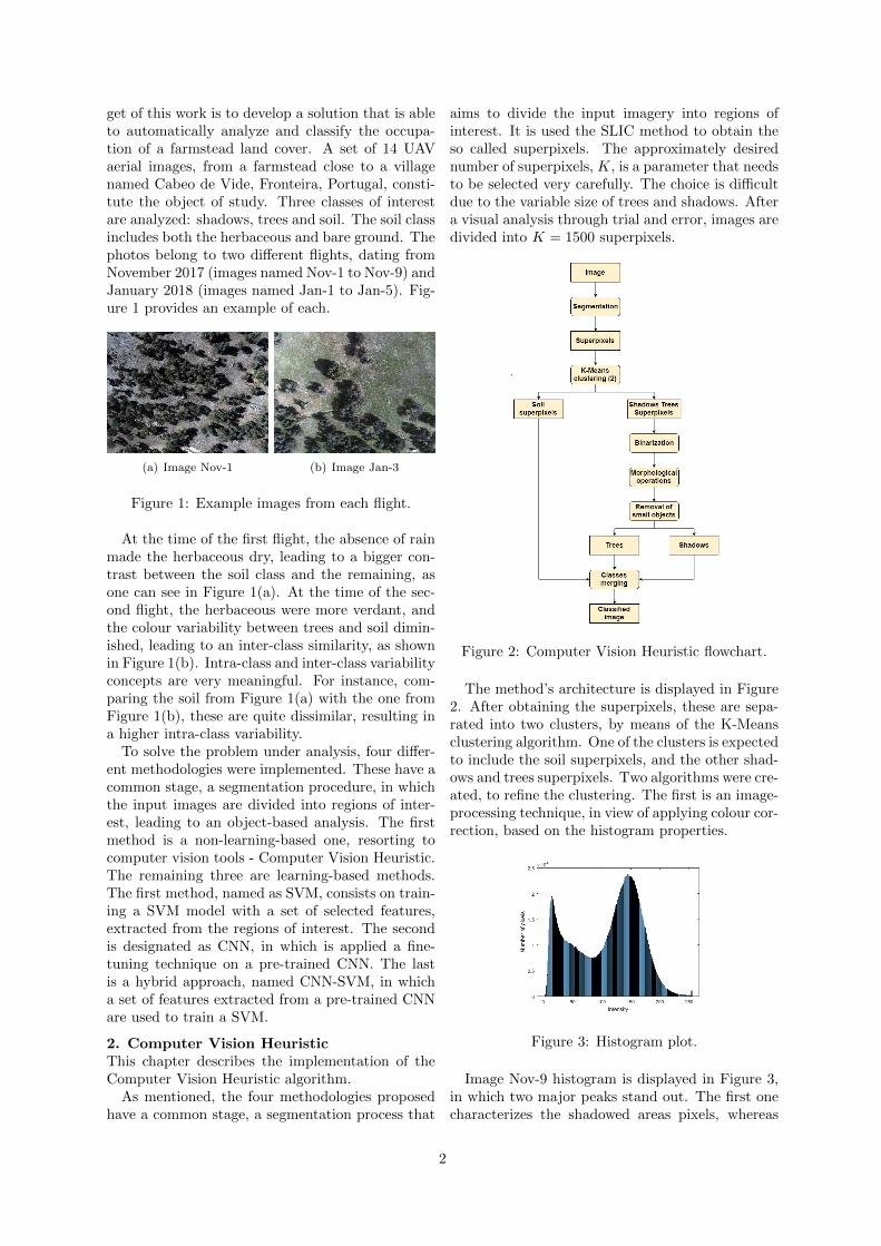
aims to divide the input imagery into regions ofinterest. It is used the SLIC method to obtain theso called superpixels. The approximately desirednumber of superpixels, K, is a parameter that needsto be selected very carefully. The choice is difficultdue to the variable size of trees and shadows. Aftera visual analysis through trial and error, images aredivided into K = 1500 superpixels.

Figure 2: Computer Vision Heuristic flowchart.

The method’s architecture is displayed in Figure2. After obtaining the superpixels, these are sepa-rated into two clusters, by means of the K-Meansclustering algorithm. One of the clusters is expectedto include the soil superpixels, and the other shad-ows and trees superpixels. Two algorithms were cre-ated, to refine the clustering. The first is an image-processing technique, in view of applying colour cor-rection, based on the histogram properties.

Figure 3: Histogram plot.

Image Nov-9 histogram is displayed in Figure 3,in which two major peaks stand out. The first onecharacterizes the shadowed areas pixels, whereas

2

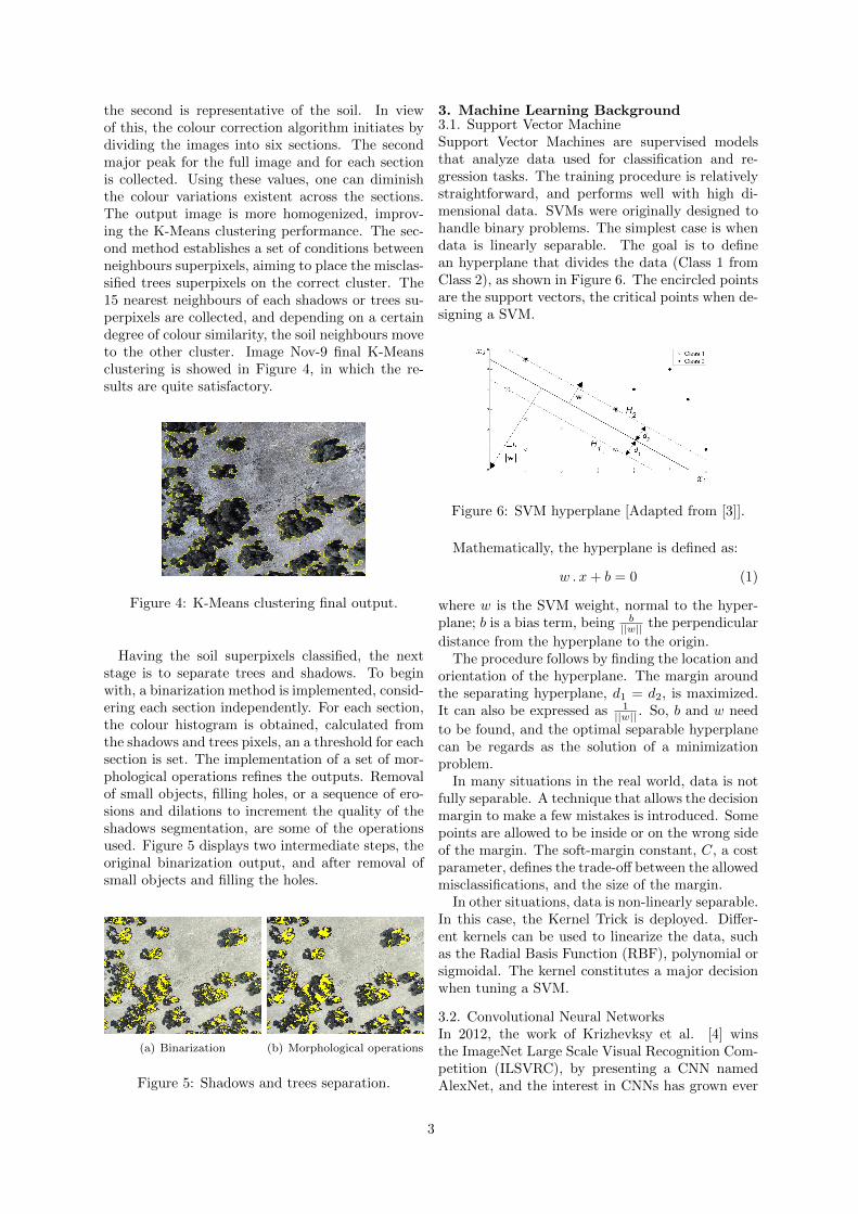
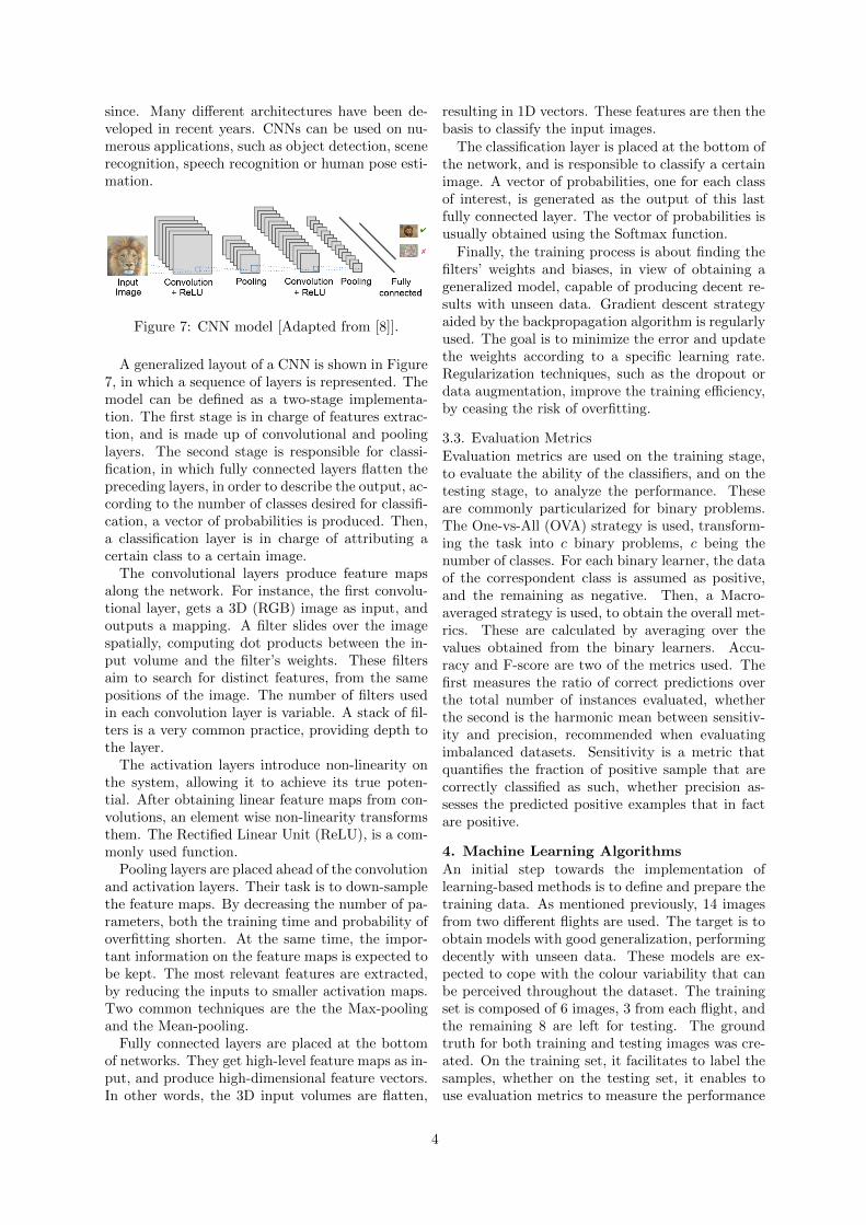
the second is representative of the soil. In viewof this, the colour correction algorithm initiates bydividing the images into six sections. The secondmajor peak for the full image and for each sectionis collected. Using these values, one can diminishthe colour variations existent across the sections.The output image is more homogenized, improv-ing the K-Means clustering performance. The sec-ond method establishes a set of conditions betweenneighbours superpixels, aiming to place the misclas-sified trees superpixels on the correct cluster. The15 nearest neighbours of each shadows or trees su-perpixels are collected, and depending on a certaindegree of colour similarity, the soil neighbours moveto the other cluster. Image Nov-9 final K-Meansclustering is showed in Figure 4, in which the re-sults are quite satisfactory.

Figure 4: K-Means clustering final output.

Having the soil superpixels classified, the nextstage is to separate trees and shadows. To beginwith, a binarization method is implemented, consid-ering each section independently. For each section,the colour histogram is obtained, calculated fromthe shadows and trees pixels, an a threshold for eachsection is set. The implementation of a set of mor-phological operations refines the outputs. Removalof small objects, filling holes, or a sequence of ero-sions and dilations to increment the quality of theshadows segmentation, are some of the operationsused. Figure 5 displays two intermediate steps, theoriginal binarization output, and after removal ofsmall objects and filling the holes.

(a) Binarization (b) Morphological operations

Figure 5: Shadows and trees separation.

3. Machine Learning Background3.1. Support Vector MachineSupport Vector Machines are supervised modelsthat analyze data used for classification and re-gression tasks. The training procedure is relativelystraightforward, and performs well with high di-mensional data. SVMs were originally designed tohandle binary problems. The simplest case is whendata is linearly separable. The goal is to definean hyperplane that divides the data (Class 1 fromClass 2), as shown in Figure 6. The encircled pointsare the support vectors, the critical points when de-signing a SVM.

Figure 6: SVM hyperplane [Adapted from [3]].

Mathematically, the hyperplane is defined as:

w . x+ b = 0 (1)

where w is the SVM weight, normal to the hyper-plane; b is a bias term, being b

||w|| the perpendicular

distance from the hyperplane to the origin.The procedure follows by finding the location and

orientation of the hyperplane. The margin aroundthe separating hyperplane, d1 = d2, is maximized.It can also be expressed as 1

||w|| . So, b and w need

to be found, and the optimal separable hyperplanecan be regards as the solution of a minimizationproblem.

In many situations in the real world, data is notfully separable. A technique that allows the decisionmargin to make a few mistakes is introduced. Somepoints are allowed to be inside or on the wrong sideof the margin. The soft-margin constant, C, a costparameter, defines the trade-off between the allowedmisclassifications, and the size of the margin.

In other situations, data is non-linearly separable.In this case, the Kernel Trick is deployed. Differ-ent kernels can be used to linearize the data, suchas the Radial Basis Function (RBF), polynomial orsigmoidal. The kernel constitutes a major decisionwhen tuning a SVM.

3.2. Convolutional Neural NetworksIn 2012, the work of Krizhevksy et al. [4] winsthe ImageNet Large Scale Visual Recognition Com-petition (ILSVRC), by presenting a CNN namedAlexNet, and the interest in CNNs has grown ever

3

since. Many different architectures have been de-veloped in recent years. CNNs can be used on nu-merous applications, such as object detection, scenerecognition, speech recognition or human pose esti-mation.

Figure 7: CNN model [Adapted from [8]].

A generalized layout of a CNN is shown in Figure7, in which a sequence of layers is represented. Themodel can be defined as a two-stage implementa-tion. The first stage is in charge of features extrac-tion, and is made up of convolutional and poolinglayers. The second stage is responsible for classi-fication, in which fully connected layers flatten thepreceding layers, in order to describe the output, ac-cording to the number of classes desired for classifi-cation, a vector of probabilities is produced. Then,a classification layer is in charge of attributing acertain class to a certain image.

The convolutional layers produce feature mapsalong the network. For instance, the first convolu-tional layer, gets a 3D (RGB) image as input, andoutputs a mapping. A filter slides over the imagespatially, computing dot products between the in-put volume and the filter’s weights. These filtersaim to search for distinct features, from the samepositions of the image. The number of filters usedin each convolution layer is variable. A stack of fil-ters is a very common practice, providing depth tothe layer.

The activation layers introduce non-linearity onthe system, allowing it to achieve its true poten-tial. After obtaining linear feature maps from con-volutions, an element wise non-linearity transformsthem. The Rectified Linear Unit (ReLU), is a com-monly used function.

Pooling layers are placed ahead of the convolutionand activation layers. Their task is to down-samplethe feature maps. By decreasing the number of pa-rameters, both the training time and probability ofoverfitting shorten. At the same time, the impor-tant information on the feature maps is expected tobe kept. The most relevant features are extracted,by reducing the inputs to smaller activation maps.Two common techniques are the the Max-poolingand the Mean-pooling.

Fully connected layers are placed at the bottomof networks. They get high-level feature maps as in-put, and produce high-dimensional feature vectors.In other words, the 3D input volumes are flatten,

resulting in 1D vectors. These features are then thebasis to classify the input images.

The classification layer is placed at the bottom ofthe network, and is responsible to classify a certainimage. A vector of probabilities, one for each classof interest, is generated as the output of this lastfully connected layer. The vector of probabilities isusually obtained using the Softmax function.

Finally, the training process is about finding thefilters’ weights and biases, in view of obtaining ageneralized model, capable of producing decent re-sults with unseen data. Gradient descent strategyaided by the backpropagation algorithm is regularlyused. The goal is to minimize the error and updatethe weights according to a specific learning rate.Regularization techniques, such as the dropout ordata augmentation, improve the training efficiency,by ceasing the risk of overfitting.

3.3. Evaluation MetricsEvaluation metrics are used on the training stage,to evaluate the ability of the classifiers, and on thetesting stage, to analyze the performance. Theseare commonly particularized for binary problems.The One-vs-All (OVA) strategy is used, transform-ing the task into c binary problems, c being thenumber of classes. For each binary learner, the dataof the correspondent class is assumed as positive,and the remaining as negative. Then, a Macro-averaged strategy is used, to obtain the overall met-rics. These are calculated by averaging over thevalues obtained from the binary learners. Accu-racy and F-score are two of the metrics used. Thefirst measures the ratio of correct predictions overthe total number of instances evaluated, whetherthe second is the harmonic mean between sensitiv-ity and precision, recommended when evaluatingimbalanced datasets. Sensitivity is a metric thatquantifies the fraction of positive sample that arecorrectly classified as such, whether precision as-sesses the predicted positive examples that in factare positive.

4. Machine Learning AlgorithmsAn initial step towards the implementation oflearning-based methods is to define and prepare thetraining data. As mentioned previously, 14 imagesfrom two different flights are used. The target is toobtain models with good generalization, performingdecently with unseen data. These models are ex-pected to cope with the colour variability that canbe perceived throughout the dataset. The trainingset is composed of 6 images, 3 from each flight, andthe remaining 8 are left for testing. The groundtruth for both training and testing images was cre-ated. On the training set, it facilitates to label thesamples, whether on the testing set, it enables touse evaluation metrics to measure the performance

4

of the models. The labelling is not 100% certain.In some situations, it is difficult to decide whichclass is represented. In others, it is hard to per-ceive the exact boundaries between a certain treeand surrounding shadows.

4.1. SVM

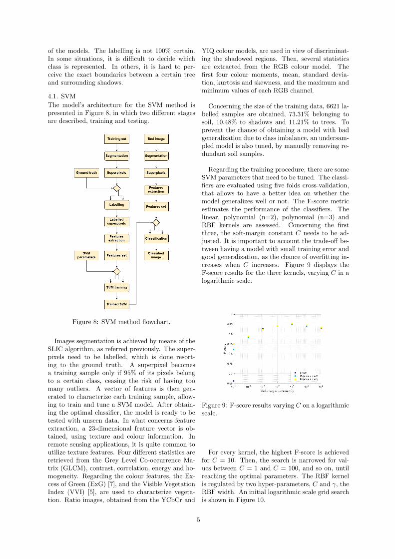
The model’s architecture for the SVM method ispresented in Figure 8, in which two different stagesare described, training and testing.

Figure 8: SVM method flowchart.

Images segmentation is achieved by means of theSLIC algorithm, as referred previously. The super-pixels need to be labelled, which is done resort-ing to the ground truth. A superpixel becomesa training sample only if 95% of its pixels belongto a certain class, ceasing the risk of having toomany outliers. A vector of features is then gen-erated to characterize each training sample, allow-ing to train and tune a SVM model. After obtain-ing the optimal classifier, the model is ready to betested with unseen data. In what concerns featureextraction, a 23-dimensional feature vector is ob-tained, using texture and colour information. Inremote sensing applications, it is quite common toutilize texture features. Four different statistics areretrieved from the Grey Level Co-occurrence Ma-trix (GLCM), contrast, correlation, energy and ho-mogeneity. Regarding the colour features, the Ex-cess of Green (ExG) [7], and the Visible VegetationIndex (VVI) [5], are used to characterize vegeta-tion. Ratio images, obtained from the YCbCr and

YIQ colour models, are used in view of discriminat-ing the shadowed regions. Then, several statisticsare extracted from the RGB colour model. Thefirst four colour moments, mean, standard devia-tion, kurtosis and skewness, and the maximum andminimum values of each RGB channel.

Concerning the size of the training data, 6621 la-belled samples are obtained, 73.31% belonging tosoil, 10.48% to shadows and 11.21% to trees. Toprevent the chance of obtaining a model with badgeneralization due to class imbalance, an undersam-pled model is also tuned, by manually removing re-dundant soil samples.

Regarding the training procedure, there are someSVM parameters that need to be tuned. The classi-fiers are evaluated using five folds cross-validation,that allows to have a better idea on whether themodel generalizes well or not. The F-score metricestimates the performance of the classifiers. Thelinear, polynomial (n=2), polynomial (n=3) andRBF kernels are assessed. Concerning the firstthree, the soft-margin constant C needs to be ad-justed. It is important to account the trade-off be-tween having a model with small training error andgood generalization, as the chance of overfitting in-creases when C increases. Figure 9 displays theF-score results for the three kernels, varying C in alogarithmic scale.

Figure 9: F-score results varying C on a logarithmicscale.

For every kernel, the highest F-score is achievedfor C = 10. Then, the search is narrowed for val-ues between C = 1 and C = 100, and so on, untilreaching the optimal parameters. The RBF kernelis regulated by two hyper-parameters, C and γ, theRBF width. An initial logarithmic scale grid searchis shown in Figure 10.

5

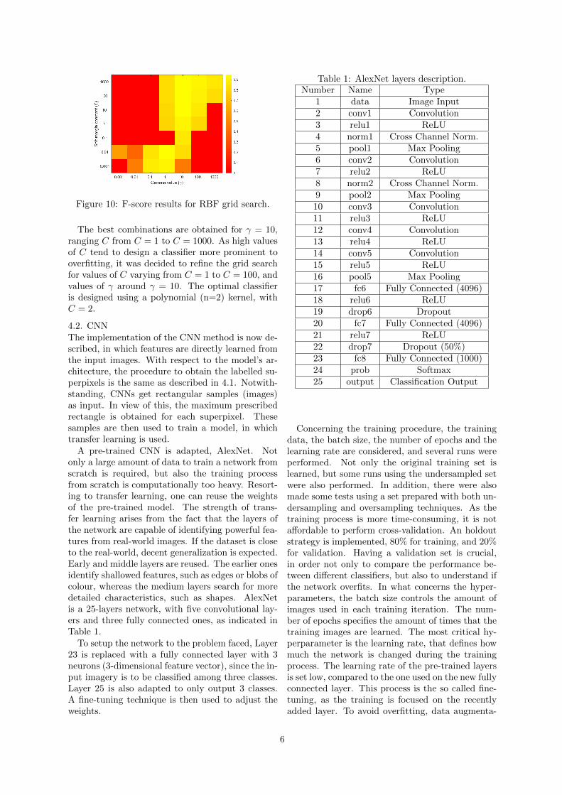
Figure 10: F-score results for RBF grid search.

The best combinations are obtained for γ = 10,ranging C from C = 1 to C = 1000. As high valuesof C tend to design a classifier more prominent tooverfitting, it was decided to refine the grid searchfor values of C varying from C = 1 to C = 100, andvalues of γ around γ = 10. The optimal classifieris designed using a polynomial (n=2) kernel, withC = 2.

4.2. CNNThe implementation of the CNN method is now de-scribed, in which features are directly learned fromthe input images. With respect to the model’s ar-chitecture, the procedure to obtain the labelled su-perpixels is the same as described in 4.1. Notwith-standing, CNNs get rectangular samples (images)as input. In view of this, the maximum prescribedrectangle is obtained for each superpixel. Thesesamples are then used to train a model, in whichtransfer learning is used.

A pre-trained CNN is adapted, AlexNet. Notonly a large amount of data to train a network fromscratch is required, but also the training processfrom scratch is computationally too heavy. Resort-ing to transfer learning, one can reuse the weightsof the pre-trained model. The strength of trans-fer learning arises from the fact that the layers ofthe network are capable of identifying powerful fea-tures from real-world images. If the dataset is closeto the real-world, decent generalization is expected.Early and middle layers are reused. The earlier onesidentify shallowed features, such as edges or blobs ofcolour, whereas the medium layers search for moredetailed characteristics, such as shapes. AlexNetis a 25-layers network, with five convolutional lay-ers and three fully connected ones, as indicated inTable 1.

To setup the network to the problem faced, Layer23 is replaced with a fully connected layer with 3neurons (3-dimensional feature vector), since the in-put imagery is to be classified among three classes.Layer 25 is also adapted to only output 3 classes.A fine-tuning technique is then used to adjust theweights.

Table 1: AlexNet layers description.Number Name Type

1 data Image Input2 conv1 Convolution3 relu1 ReLU4 norm1 Cross Channel Norm.5 pool1 Max Pooling6 conv2 Convolution7 relu2 ReLU8 norm2 Cross Channel Norm.9 pool2 Max Pooling10 conv3 Convolution11 relu3 ReLU12 conv4 Convolution13 relu4 ReLU14 conv5 Convolution15 relu5 ReLU16 pool5 Max Pooling17 fc6 Fully Connected (4096)18 relu6 ReLU19 drop6 Dropout20 fc7 Fully Connected (4096)21 relu7 ReLU22 drop7 Dropout (50%)23 fc8 Fully Connected (1000)24 prob Softmax25 output Classification Output

Concerning the training procedure, the trainingdata, the batch size, the number of epochs and thelearning rate are considered, and several runs wereperformed. Not only the original training set islearned, but some runs using the undersampled setwere also performed. In addition, there were alsomade some tests using a set prepared with both un-dersampling and oversampling techniques. As thetraining process is more time-consuming, it is notaffordable to perform cross-validation. An holdoutstrategy is implemented, 80% for training, and 20%for validation. Having a validation set is crucial,in order not only to compare the performance be-tween different classifiers, but also to understand ifthe network overfits. In what concerns the hyper-parameters, the batch size controls the amount ofimages used in each training iteration. The num-ber of epochs specifies the amount of times that thetraining images are learned. The most critical hy-perparameter is the learning rate, that defines howmuch the network is changed during the trainingprocess. The learning rate of the pre-trained layersis set low, compared to the one used on the new fullyconnected layer. This process is the so called fine-tuning, as the training is focused on the recentlyadded layer. To avoid overfitting, data augmenta-

6

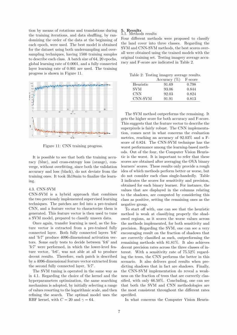
tion by means of rotations and translations duringthe training iterations, and data shuffling, by ran-domizing the order of the data at the beginning ofeach epoch, were used. The best model is obtainedfor the dataset using both undersampling and over-sampling techniques, having 1500 training samplesto describe each class. A batch size of 64, 20 epochs,global learning rate of 0.0001, and a fully connectedlayer learning rate of 0.001 are used. The trainingprogress is shown in Figure 11.

Figure 11: CNN training progress.

It is possible to see that both the training accu-racy (blue), and cross-entropy loss (orange), con-verge, without overfitting, since both the validationaccuracy and loss (black), do not deviate from thetraining ones. It took 3h18min to finalize the learn-ing.

4.3. CNN-SVM

CNN-SVM is a hybrid approach that combinesthe two previously implemented supervised learningtechniques. The patches are fed into a pre-trainedCNN, and a feature vector to characterize them isgenerated. This feature vector is then used to tunea SVM model, prepared to classify unseen data.

Once again, transfer learning is used, as the fea-ture vector is extracted from a pre-trained fullyconnected layer. Both fully connected layers ’fc6’and ’fc7’ produce 4096-dimensional activation vec-tors. Some early tests to decide between ’fc6’ and’fc7’ were performed, in which the lower-level fea-ture vector, ’fc6’, was not able at all to producedecent results. Therefore, each patch is describedby a 4096-dimensional feature vector extracted fromthe second fully connected layer, ’fc7’.

The SVM tuning is operated in the same way asin 4.1. Regarding the choice of the kernel and thehyperparameters optimization, the same searchingmechanism is adopted, by initially selecting a rangeof values resorting to the logarithmic scale, and thenrefining the search. The optimal model uses theRBF kernel, with C = 20 and γ = 64.

5. Results5.1. Methods resultsFour different methods were proposed to classifythe land cover into three classes. Regarding theSVM and CNN-SVM methods, the best scores over-all were obtained using the trained models with theoriginal training set. Testing imagery average accu-racy and F-score are indicated in Table 2.

Table 2: Testing imagery average results.Accuracy (%) F-score

Heuristic 91.69 0.798SVM 93.06 0.844CNN 92.03 0.824CNN-SVM 91.91 0.813

The SVM method outperforms the remaining. Itgets the higher score for both accuracy and F-score.This suggests that the feature vector to describe thesuperpixels is fairly robust. The CNN implementa-tion, comes next in what concerns the evaluationmetrics, reaching an accuracy of 92.03% and a F-score of 0.824. The CNN-SVM technique has theworst performance among the learning-based meth-ods. Out of the four, the Computer Vision Heuris-tic is the worst. It is important to refer that thesescores are obtained after averaging the OVA binarylearners’ scores. These results only provide a roughidea of which methods perform better or worse, butdo not consider each class single-handedly. Table3 indicates the scores for sensitivity and precision,obtained for each binary learner. For instance, thevalues that are displayed in the columns relatingto the shadows, are computed by considering thisclass as positive, setting the remaining ones as thenegative group.

To start off with, one can see that the heuristicmethod is weak at classifying properly the shad-owed regions, as it scores the worse values acrossthe methods implemented, for both sensitivity andprecision. Regarding the SVM, one can see a veryencouraging result on the fraction of shadows thatare correctly classified as such, outperforming theremaining methods with 81.81%. It also achievesdecent precision rates across the three classes of in-terest. With a sensitivity rate of 75.52% regard-ing the trees, the CNN performs the better in thisscenario. It also delivers good results when pre-dicting shadows that in fact are shadows. Finally,the CNN-SVM implementation do reveal a weak-ness on the fraction of trees that are correctly clas-sified, with only 66.50%. Concluding, one can seethat both the SVM and CNN methodologies arethe most consistent throughout the different ratesspecified.

In what concerns the Computer Vision Heuris-

7

Table 3: Testing imagery average sensitivity and precision rates, obtained from each One-vs-All binaryclassifier, for the four methods implemented.

Sensitivity (%) Precision (%)

Shadow Tree Soil Shadow Tree Soil

Heuristic 66.57 72.61 96.22 78.81 71.51 93.21

SVM 81.81 70.99 96.93 82.04 81.91 92.81

CNN 73.58 75.52 94.99 84.82 73.00 92.92

CNN-SVM 76.70 66.50 96.70 80.44 75.48 92.14

tic, the classification is poor when testing the Jan-uary images. An accuracy of 93.06% and a F-scoreof 0.843 are obtained when classifying the Novem-ber images, achieving similar values to the ones ob-tained on the SVM method. On the other hand,for the January imagery, the accuracy diminishesto 88.00%, and the F-score to 0.682. Image Jan-5,displayed in Figure 12, is analyzed in detail.

Figure 12: Image Jan-5.

(a) Ground truth (b) Classification map

Figure 13: Computer Vision Heuristic classificationanalysis, for image Jan-5.

Figure 13 shows the ground truth and classifi-cation maps obtained. One can visualize that themethod is not capable of correctly identifying shad-ows, with only 14.19% being correctly predicted.On the other hand, the soil is decently segmented,with 97.55% of the pixels being correctly classified.As the name induces, the concept of heuristic is in-troduced since the method works for a set of images,but is not guaranteed to work on others. The tech-nique was initially prepared to classify the Novem-ber set. As mentioned, the threshold to separatetrees and shadows is obtained via colour histogram,

and a constant is added at a given point. This iswhere the root cause is. The discrepancy in termsof colour between trees and shadows is not so pro-nounced in the January set, which ultimately dam-ages the results obtained.

Image Nov-4, displayed in Figure 14, classifica-tion through the SVM method is showed in Figure15. The ground truth and the classification mapseem fairly similar. There are still some regions thatare misclassified, mainly soil areas that are coveredwith shrubs. This issue is in fact a topic for discus-sion, since the classification task does not includethe identification of this vegetation extract. Thepossibility of these superpixels being misclassifiedis higher, as the colour distribution is closer to thetrees.

Figure 14: Image Nov-4.

(a) Ground truth (b) Classification map

Figure 15: SVM classification analysis, for imageNov-4.

5.2. Temporal Variability AnalysisThe impact of temporal variability, in which is stud-ied the effect of the time of the year in which the im-ages are collected, is now discussed. The learning-

8

based methods were designed using training datafrom both flights. To study the temporal vari-ability, additional models were designed. For eachlearning-based technique, two different models wereobtained, one from each training set (Nov-2, Nov-3,Nov-6 and Jan-2, Jan-3, Jan-5). These new mod-els are evaluated using testing imagery from eachflight. The results obtained for the SVM methodare now analyzed, particularizing the F-score val-ues, indicated in Table 4.

Table 4: SVM temporal variability analysis F-score.Train-Nov Train-Jan Train-All

Test-Nov 0.860 0.781 0.853Test-Jan 0.519 0.806 0.817

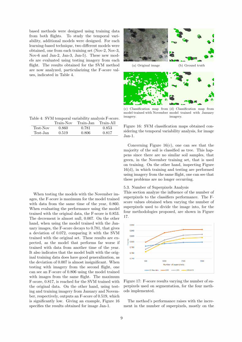
When testing the models with the November im-ages, the F-score is maximum for the model trainedwith data from the same time of the year, 0.860.When evaluating the performance using the modeltrained with the original data, the F-score is 0.853.The decrement is almost null, 0.007. On the otherhand, when using the model trained with the Jan-uary images, the F-score decays to 0.781, that givesa deviation of 0.072, comparing it with the SVMtrained with the original set. These results are ex-pected, as the model that performs far worse iftrained with data from another time of the year.It also indicates that the model built with the orig-inal training data does have good generalization, asthe deviation of 0.007 is almost insignificant. Whentesting with imagery from the second flight, onecan see an F-score of 0.806 using the model trainedwith images from the same flight. The maximumF-score, 0.817, is reached for the SVM trained withthe original data. On the other hand, using test-ing and training imagery from January and Novem-ber, respectively, outputs an F-score of 0.519, whichis significantly low. Giving an example, Figure 16specifies the results obtained for image Jan-1.

(a) Original image (b) Ground truth

(c) Classification map frommodel trained with Novemberimagery.

(d) Classification map frommodel trained with Januaryimagery.

Figure 16: SVM classification maps obtained con-sidering the temporal variability analysis, for imageJan-1.

Concerning Figure 16(c), one can see that themajority of the soil is classified as tree. This hap-pens since there are no similar soil samples, thatgreen, in the November training set, that is usedon training. On the other hand, inspecting Figure16(d), in which training and testing are performedusing imagery from the same flight, one can see thatthese problems are no longer occurring.

5.3. Number of Superpixels AnalysisThis section analyze the influence of the number ofsuperpixels to the classifiers performance. The F-score values obtained when varying the number ofsuperpixels used to divide the image into, for thefour methodologies proposed, are shown in Figure17.

Figure 17: F-score results varying the number of su-perpixels used on segmentation, for the four meth-ods implemented.

The method’s performance raises with the incre-ment in the number of superpixels, mostly on the

9

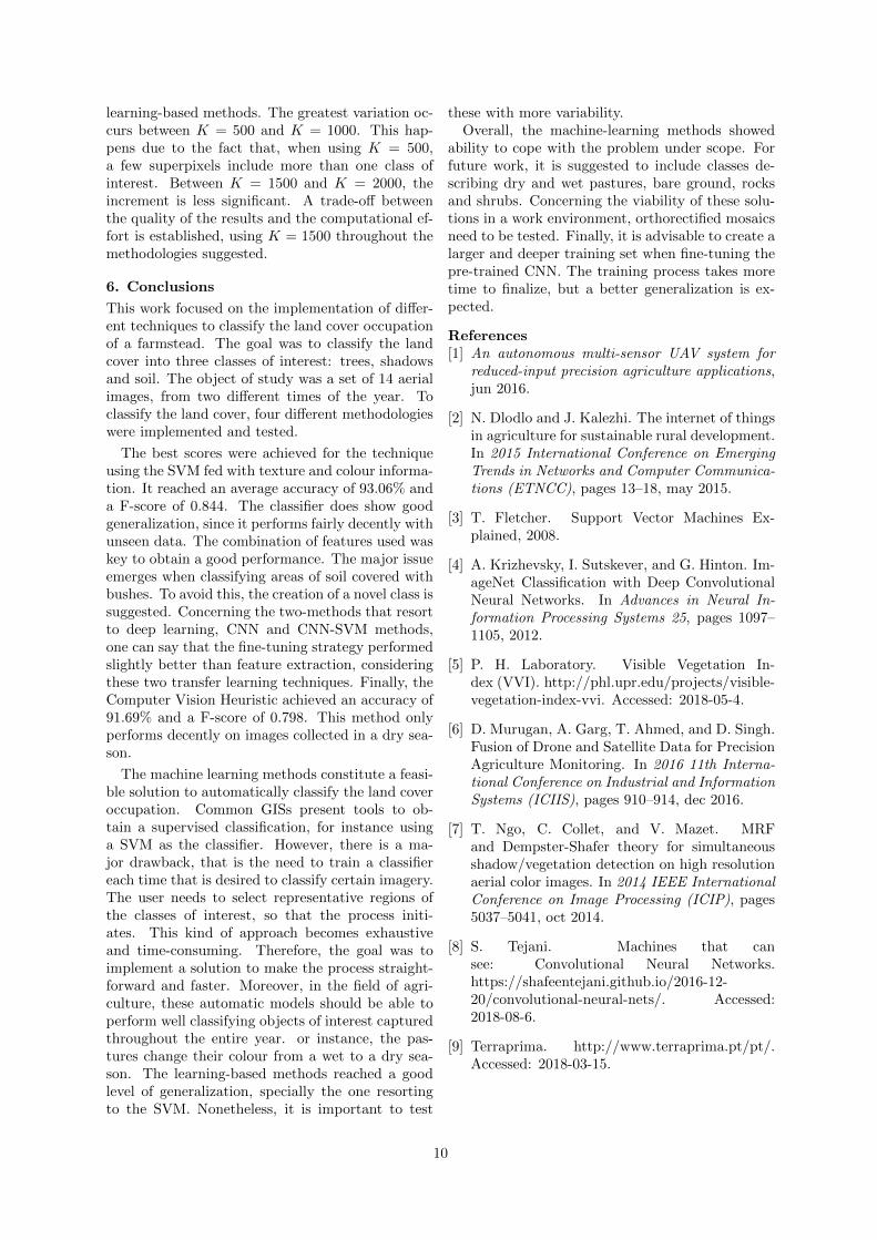
learning-based methods. The greatest variation oc-curs between K = 500 and K = 1000. This hap-pens due to the fact that, when using K = 500,a few superpixels include more than one class ofinterest. Between K = 1500 and K = 2000, theincrement is less significant. A trade-off betweenthe quality of the results and the computational ef-fort is established, using K = 1500 throughout themethodologies suggested.

6. Conclusions

This work focused on the implementation of differ-ent techniques to classify the land cover occupationof a farmstead. The goal was to classify the landcover into three classes of interest: trees, shadowsand soil. The object of study was a set of 14 aerialimages, from two different times of the year. Toclassify the land cover, four different methodologieswere implemented and tested.

The best scores were achieved for the techniqueusing the SVM fed with texture and colour informa-tion. It reached an average accuracy of 93.06% anda F-score of 0.844. The classifier does show goodgeneralization, since it performs fairly decently withunseen data. The combination of features used waskey to obtain a good performance. The major issueemerges when classifying areas of soil covered withbushes. To avoid this, the creation of a novel class issuggested. Concerning the two-methods that resortto deep learning, CNN and CNN-SVM methods,one can say that the fine-tuning strategy performedslightly better than feature extraction, consideringthese two transfer learning techniques. Finally, theComputer Vision Heuristic achieved an accuracy of91.69% and a F-score of 0.798. This method onlyperforms decently on images collected in a dry sea-son.

The machine learning methods constitute a feasi-ble solution to automatically classify the land coveroccupation. Common GISs present tools to ob-tain a supervised classification, for instance usinga SVM as the classifier. However, there is a ma-jor drawback, that is the need to train a classifiereach time that is desired to classify certain imagery.The user needs to select representative regions ofthe classes of interest, so that the process initi-ates. This kind of approach becomes exhaustiveand time-consuming. Therefore, the goal was toimplement a solution to make the process straight-forward and faster. Moreover, in the field of agri-culture, these automatic models should be able toperform well classifying objects of interest capturedthroughout the entire year. or instance, the pas-tures change their colour from a wet to a dry sea-son. The learning-based methods reached a goodlevel of generalization, specially the one resortingto the SVM. Nonetheless, it is important to test

these with more variability.Overall, the machine-learning methods showed

ability to cope with the problem under scope. Forfuture work, it is suggested to include classes de-scribing dry and wet pastures, bare ground, rocksand shrubs. Concerning the viability of these solu-tions in a work environment, orthorectified mosaicsneed to be tested. Finally, it is advisable to create alarger and deeper training set when fine-tuning thepre-trained CNN. The training process takes moretime to finalize, but a better generalization is ex-pected.

References[1] An autonomous multi-sensor UAV system for

reduced-input precision agriculture applications,jun 2016.

[2] N. Dlodlo and J. Kalezhi. The internet of thingsin agriculture for sustainable rural development.In 2015 International Conference on EmergingTrends in Networks and Computer Communica-tions (ETNCC), pages 13–18, may 2015.

[3] T. Fletcher. Support Vector Machines Ex-plained, 2008.

[4] A. Krizhevsky, I. Sutskever, and G. Hinton. Im-ageNet Classification with Deep ConvolutionalNeural Networks. In Advances in Neural In-formation Processing Systems 25, pages 1097–1105, 2012.

[5] P. H. Laboratory. Visible Vegetation In-dex (VVI). http://phl.upr.edu/projects/visible-vegetation-index-vvi. Accessed: 2018-05-4.

[6] D. Murugan, A. Garg, T. Ahmed, and D. Singh.Fusion of Drone and Satellite Data for PrecisionAgriculture Monitoring. In 2016 11th Interna-tional Conference on Industrial and InformationSystems (ICIIS), pages 910–914, dec 2016.

[7] T. Ngo, C. Collet, and V. Mazet. MRFand Dempster-Shafer theory for simultaneousshadow/vegetation detection on high resolutionaerial color images. In 2014 IEEE InternationalConference on Image Processing (ICIP), pages5037–5041, oct 2014.

[8] S. Tejani. Machines that cansee: Convolutional Neural Networks.https://shafeentejani.github.io/2016-12-20/convolutional-neural-nets/. Accessed:2018-08-6.

[9] Terraprima. http://www.terraprima.pt/pt/.Accessed: 2018-03-15.

10